Abstract
Fugitive dust is an important source of total suspended particulate matter in urban ambient air. The existing segmentation methods for dust sources face challenges in distinguishing key and secondary features, and they exhibit poor segmentation at the image edge. To address these issues, this paper proposes the Dust Source U-Net (DSU-Net), enhancing the U-Net model by incorporating VGG16 for feature extraction, and integrating the shuffle attention module into the jump connection branch to enhance feature acquisition. Furthermore, we combine Dice Loss, Focal Loss, and Activate Boundary Loss to improve the boundary extraction accuracy and reduce the loss oscillation. To evaluate the effectiveness of our model, we selected Jingmen City, Jingzhou City, and Yichang City in Hubei Province as the experimental area and established two dust source datasets from 0.5 m high-resolution remote sensing imagery acquired by the Jilin-1 satellite. Our created datasets include dataset HDSD-A for dust source segmentation and dataset HDSD-B for distinguishing the dust control measures. Comparative analyses of our proposed model with other typical segmentation models demonstrated that our proposed DSU-Net has the best detection performance, achieving a mIoU of 93% on dataset HDSD-A and 92% on dataset HDSD-B. In addition, we verified that it can be successfully applied to detect dust sources in urban areas.
1. Introduction
China has made significant improvements in controlling air pollution, particularly in reducing haze weather [1]. At the end of 2023, to further promote the ongoing improvement of air quality, the government released the latest “Action Plan for Continuous Improvement of Air Quality”. This plan sets a target for a 10% reduction in the concentration of PM2.5 in cities at the prefecture level and above by 2025, compared to 2020 levels. The causes and effects of haze weather, particularly the surge in suspended particulate matter in the air [2], have gained widespread attention across various sectors. Open sources of urban particulate matter, referred to as fugitive dust sources [3], are important pollutants affecting the quality of the urban air environment. According to the “Technical Guidelines for the Preparation of Particulate Matter Emission Inventories for Dust Sources (for Trial Implementation)” [4], dust sources can be classified into soil dust, road dust, construction dust and landfill dust, among which soil dust refers to the particulate matter directly originating from the bare ground formed by the activities of nature or manpower. Road dust refers to the dust accumulated on the road that enters the air by wind, vehicle driving, or crowd activities. Construction dust refers to the dust generated during the construction of various facilities in the city. Yard dust refers to the dust caused by various industrial material piles, construction material piles, and waste residue after stacking, transporting, loading, and other operations. Most of the exposed dust sources and bare land to be constructed are located within the main urban areas of the city, which are usually surrounded by densely populated areas [5]. Therefore, it is of great significance to accurately grasp the distribution information of urban fugitive dust sources for effective pollution prevention and environmental regulation to improve urban air quality.
Optical satellite remote sensing, because of its wide coverage, has become a better choice for monitoring dust sources at construction sites and bare ground. In recent years, researchers across the world have carried out diverse studies on dust source pollution monitoring, such as optimising the calculation methods of particulate emissions from dust sources and the spatial detection analysis of dust sources. Behzad Rayegani et al. [6] introduced a data-driven approach to study the air quality problems associated with dust from the surface of coal mines. The approach was to install air quality detectors at different locations around the coal mine to obtain real-time data, which were later integrated with an air-quality-monitoring system. Zhang et al. [7] investigated the emission characteristics of microplastics emitted to the atmosphere from road dust in a mine site and redefined the emission factors of microplastics from road dust sources to establish a new emission inventory. Katheryn R. Kolesar et al. [8] used stratified sampling of dust sources in the Keeler dunes to assess the potential PM10 fluxes in different terrains based on high-resolution satellite imagery and ground-based observations, and deduced that alluvial landscapes are the main source of dust emissions. Zhao et al. [9] proposed a method for predicting the spreading range of pollutants from building demolition based on the Euclidean distance transform to address the problem of low prediction accuracy in pollutant spreading range prediction. There are also some researchers who directly analyse dust particles. For example, Behzad Rayegani et al. [10] first used Landsat8 satellite data to obtain wind erosion sensitivity maps after preprocessing and classifying spectral vegetation indices. This was followed by collecting weather data and using statistical analysis and MODIS data to identify localised dust events. Yu et al. [11] used the NASA MCD19A2 dataset to analyse the aerosol optical thickness of Dexing City in 2020–2021 so as to explore its mine dust pollution status. Xu et al. [12] established a gas–solid two-phase coupled flow and thermal infrared transport model by integrating the infrared features of dynamic dust and high-temperature exhaust coupling phenomena. The intrinsic mechanisms of particle size and concentration of particles caused by vehicle dust and their influence on the infrared signatures were investigated.
Benefiting from the rapid development of remote sensing technology, satellite remote sensing can be used to obtain global ground information more comprehensively and quickly. Recently, deep learning combined with remote sensing images has become a research hotspot. Significant research efforts have been dedicated to remote sensing image detection tasks, particularly in the field of semantic segmentation. For example, the extraction of buildings and roads [13,14,15], photovoltaic panel detection [16,17], oil tank detection [18,19], oil infrastructure detection [20,21,22,23], and farmed net detection [24,25] in remote sensing images. Sun et al. [26] proposed a hybrid multiresolution and transformer semantic extraction network that overcomes the problem of small receptive fields in convolutional neural networks to fully extract feature information. Zeng et al. [27] used the Gaofen-2 satellite as the research object, and the recognition accuracy was much higher than the traditional image recognition model when using a CNN to recognise remote sensing images. The BOMSC-Net method proposed by Yuan et al. [28] considers the boundary optimisation and multi-scale context-awareness problems and focuses more on boundary quality. The complex texture of optical remote sensing images, which contain rich feature information such as shape, location, and boundary, often leads to the low segmentation accuracy of remote sensing images. To cope with the challenge of low segmentation accuracy, the application of various attention mechanisms [29,30,31,32] has become a preferred strategy. Sun et al. [33] proposed Multiple Attention-based U-Net (MA-UNet), which uses channel attention and spatial attention at different feature fusion stages to better fuse the feature information of the target at different scales and solve the problem of poor accuracy in different categories. Yuan et al. [34] proposed a multi-scale hierarchical channel attention fusion network model (MCAFNet) for the transformer and CNN. In the decoder, a channel attention optimisation module and a fusion module are added to enhance the network’s ability to extract feature semantic information. Wang et al. [35] improved DeepLabV3+ by using the class feature attention module to enhance the correlation between classes in order to better extract the semantic features of different classes, thus improving the segmentation accuracy.
Meanwhile, we investigate methods related to the automatic detection of dust sources using high-resolution remote sensing images. Wu et al. [36] proposed an efficient and lightweight model STAE-MobileVIT based on a CNN and transformer, which is used to segment the change area of dust sources of bare land types. He et al. [37] conducted an experimental area in Wuhai City, China, using high-resolution remote sensing images from the Gaofen-1 satellite to identify urban dust sources using U-Net and FCN, and obtained a mean Intersection over Union (mIoU) of 0.813. Asanka et al. [38] used several deep-learning-based semantic segmentation methods to quantify traffic-induced road dust and compared the segmentation predictions with the corresponding field measurements, demonstrating the potential in realistic scenarios. The method directly segments the dust itself, and it is more effective in detecting road dust occurring on bare ground, but less effective in detecting road dust occurring on tarmac roads in urban areas. In addition, dust pollution can be reduced due to the use of green plastic covers (GPCs). Some researchers have started to study dust source identification methods with dust control measures. Liu et al. [39] used a multi-scale deformable convolutional neural network to identify and map dust sources with green plastic covers in high-resolution remote sensing images. Cao et al. [40] utilised a classification-then-segmentation strategy to detect green plastic covers in high-resolution remote sensing images from Google Earth and Gaofen-2, which effectively alleviated the problem of boundary blurring in the segmentation results. Guo et al. [41] first selected a variety of machine learning methods to classify the land cover, and then used a deep learning method to predict the segmentation of green plastic covers in the images of the experimental area. However, the prediction time was longer in this way.
As can be seen from the above, there are relatively few studies on the automatic detection of urban dust sources using high-resolution optical remote sensing satellites. This study aims to enhance detection accuracy and gain insights into how dust control measures impact accuracy. This work specifically concentrates on refining the detection algorithm to improve the overall accuracy of the model. In this work, we used high-resolution remote sensing images from the Jilin-1 satellite to construct two fugitive dust source datasets using Yichang City, Jingmen City, and Jingzhou City in Hubei Province, China as experimental areas. In order to improve the segmentation accuracy of dust sources, we propose a remote sensing image segmentation model with improved U-Net, called DSU-Net. The feature extraction module is replaced by VGG16 to improve the model’s ability to capture and represent intricate features. The shuffle attention module [42] is introduced in the network, and shuffle units are used in the feature extraction module to combine channel attention and spatial attention to increase the ability of feature extraction and reduce the problem of detail information loss. Furthermore, to improve the unclear boundary of segmentation results, we fuse Dice Loss, Focal Loss, and Active Boundary Loss [43] to reduce the loss fluctuation and improve the performance of the network model. The main contribution of this paper is as follows:
- (1)
- Taking Yichang City, Jingmen City, and Jingzhou City in Hubei Province, China, as the experimental area, two high-resolution remote sensing datasets of fugitive dust sources are constructed, including dataset HDSD-A for dust source segmentation and dataset HDSD-B for distinguishing dust control measures.
- (2)
- Based on the U-Net network, the feature extraction module is replaced by VGG16, and the shuffle attention module is introduced to suppress unnecessary features and noise for better extracting the feature information of dust sources.
- (3)
- Introducing Active Boundary Loss, while combining Dice Loss and Focal Loss to improve the segmentation accuracy at the boundary.
2. Datasets
2.1. Overview of the Study Area
The cities of Jingmen, Jingzhou, and Yichang are all important members of the city cluster in the middle reaches of the Yangtze River, where a range of industrial activities, particularly construction and manufacturing, generate large quantities of dust, which has an impact on air quality. Moreover, as the Yangtze River is the longest river in China, the health of its ecosystem is critical to neighbouring cities. Dust lifting may have a negative impact on the ecosystem in and around the river, making it an important task for these cities to reduce pollution of the Yangtze River from dust lifting. Jingmen City is located in the central part of Hubei Province, in the middle and lower reaches of the Han River, between longitude 111°51′~113°29′E and latitude 30°32′~31°36′N. Jingmen City is high in the east, west, and north, low in the middle and south, and is open to the south, with both low mountain depression and valley areas, hill and gully areas, and plains and lakes. Jingzhou City is located in the south-central part of Hubei Province, the middle reaches of the Yangtze River and the hinterland of the Jianghan Plain, between longitude 111°15′~114°05′E and latitude 29°26′~31°37′N. The topography is slightly high in the west and low in the east. The terrain is slightly higher in the west and lower in the east, with a gradual transition from low hills to highlands and plains. Yichang City is in southwestern Hubei, at the boundary between the upper and middle reaches of the Yangtze River, straddling longitude 110°15′~112°04′E and latitude 29°56′–31°34′N. The terrain of Yichang City is more complex, and the height difference is huge, showing a gradual decline from the west to the east of the trend. The average slope drop is 14.5%, and the formation of mountains (high mountains, semi-high mountains, and low mountains), hills, and plains are the three major base geomorphological types. Among them, the distribution map of dust sources in Jingmen city is shown in Figure 1a, the distribution map in Jingzhou city is shown in Figure 1b, and the distribution map in Yichang city is shown in Figure 1c.
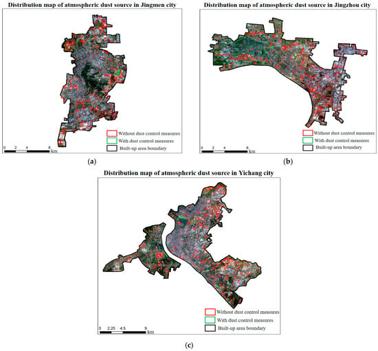
Figure 1.
The study areas: (a) Jingmen City, China; (b) Jingzhou City, China; (c) Yichang City, China. The red rectangular boxes indicate dust source patches without dust control measures and the green rectangular boxes indicate dust source patches with dust control measures. The black box indicates the built-up area boundary of the city.
2.2. Data Source
Jilin-1 is China’s first fully independently developed 0.5-metre commercial satellite system. Jilin-1 satellite remote sensing data are of sub-meter resolution, meeting the visual discernment requirement for extracting interpretive signs of dust sources by the human eye. Based on the satellite remote sensing images, the dust sources within the above three urban areas were extracted, as well as the statistical information of the dust source patches, with a monitoring area of more than 800 m2. Table 1 provides the count of dust source patches and their cumulative area for each city.

Table 1.
Statistics of dust source patches in Jingmen City, Jingzhou City, and Yichang City, Hubei Province.
In order to be capable of quickly detecting the distribution of urban dust sources, we unified the different types of dust source patches, manually deciphered in Table 1, as one large class of dust sources. They can be further divided into two different types of dust source patches, i.e., dust source patches with dust source control measures and dust source patches without dust source control measures. There are 7 patches in Jingmen City, 15 patches in Jingzhou City, and 24 patches in Yichang City with dust control measures. For dust source patches without net film coverage or with inadequate dust control measures, there are 296 in Jingmen City, 294 in Jingzhou City, and 324 in Yichang City. Using high-resolution remote sensing images from the Jilin-1 satellite, we constructed a dust source dataset HDSD-A for segmenting the dust source patches without dust control measures and a dust source dataset HDSD-B for the segmentation of a dust source with and without dust control measures. To preprocess the dataset, we used ArcGIS tools for the two datasets. For dataset HDSD-A, we labelled 507 images with a total of 960 dust sources in the three cities. For dataset HDSD-B, we labelled 166 images with a total of 46 original dust sources with dust control measures. Additionally, 914 dust sources without dust control measures in the original dataset were subjected to the same process to obtain 341 pairs of images and labels.
To make the samples more balanced, data enhancement operations were undertaken. For dataset HDSD-A, a counterclockwise rotation of 90°, 180°, and then horizontal flip operations were performed, which resulted in a 4-fold augmentation; for dataset HDSD-B, the images with dust control measures were augmented by 6-fold, and the images without dust control measures were augmented by 4-fold. Finally, dataset HDSD-A covered 2028 images, of which 1620 were in the training set and 408 were in the test set. Dataset HDSD-B, for differentiating dust control, covered 2360 images, of which 1700 were in the training set, 424 were in the validation set, and 236 were in the test set. All images in both datasets had a resolution of 0.5 m and an image size of 1600 × 1600 pixels. Figure 2 shows some example images of dust source types in three urban areas in Hubei Province. Figure 3a shows an example of dataset HDSD-A, and Figure 3b shows an example of dataset HDSD-B, which distinguishes dust control measures.
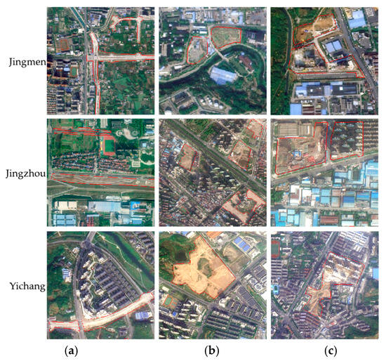
Figure 2.
Some example images of dust source types in the three urban areas of Hubei Province. (a) road construction, (b) bare ground, and (c) construction site.

Figure 3.
(a) An example image of the dust source dataset HDSD-A, where the white part is the dust source target, and the black part is the background. (b) An example image of the dust source dataset HDSD-B with dust control measures, where the white part is the dust source without dust control measures, the grey part is the dust source with dust control measures, and the black part is the background.
3. Methods
3.1. Improved U-Net Network Architecture
U-Net [44] is a symmetric codec architecture. The encoder initially down-samples the input image to extract the contextual information of the image while reducing the resolution of the feature map. The main goal of the decoder is to pinpoint and increase the feature map resolution. Finally, the pixel-level semantic segmentation results are obtained via softmax activation function. The U-Net network can combine shallow features, but it is easy to lose the detailed features in the down-sampling process, and the simple jump-joining mechanism cannot fuse the shallow features with the deeper ones well, which leads to a less satisfactory segmentation result. Therefore, we propose an improved U-Net network in this work, which is named Dust Segmentation U-Net (DSU-Net). As shown in Figure 4, we first replace the feature extraction module of U-Net with the VGG16 [45] network. The input image passes through five residual modules at a time, and the first two residual modules undergo two convolution operations with a convolution kernel size of 3 × 3, followed by a maximum pooling operation with a pooling window size of 2 × 2 and a step size of two. The last three residual modules undergo one more convolution operation than the former. After each residual module, the image size is halved, and the number of channels is doubled. Each residual module outputs four scales of feature maps in turn, which enter the shuffle attention (SA) module [42] in the jump-joining branch, and then are spliced with the feature maps obtained from the corresponding up-sampling. The decoder part maintains the original structure of U-Net, and finally obtains an effective feature layer that incorporates all the features and restores the feature map to the original input image size to obtain the pixel-level segmentation results.
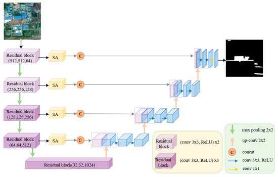
Figure 4.
Diagram of the proposed DSU-Net network architecture. We replace the feature extraction network counterpart of U-Net with VGG16, which is divided into five residual modules, and the SA attention mechanism is added to the jump connection branch, after which the feature map is spliced. The decoder maintains the original structure of U-Net.
3.2. Attention Module
SA [42] introduces the channel shuffling operation when computing attention to achieve the interaction and integration of cross-channel information, and the effect is shown in Figure 5. This method can effectively improve the expression ability of the model when processing features and increase the global understanding of features by the network. The main implementation steps of SA include:

Figure 5.
Module overview diagram of the SA attention module.
Feature grouping: First, the input feature map is X ∈ RCxHxW, where C, H, and W denote the channel number, height, and width, respectively. X is divided into G groups of sub-feature maps along the channel dimension Xk ∈ RC/GxHxW. Then, before entering the attention unit, each sub-feature map is divided into two branches Xk1, Xk2 along the channel dimension, where Xk1 is used to generate the channel attention map and Xk2 is used to obtain the spatial attention map.
Channel attention: Channel statistic c is generated using global average pooling (GAP) to embed global information [46]. Afterwards, the features are compacted by a simple gating mechanism φ activated by a sigmoid.
where Fc (·) is used to enhance the statistical representation, and two parameters, W and b, are used to perform scaling and shifting of the channel vectors.
Spatial attention: the group paradigm GN [47] is used to obtain the spatial statistic s. The same method is then used for compact features.
Feature fusion: The two branches Xk1 and Xk2 are connected. After that, all sub-features are aggregated. Finally, the spatial attention features computed within the above groups are shuffled in the channel dimension using the “channel shuffle” operation, so that information can be exchanged between different groups.
Spatial attention and channel attention aim to capture pixel-level pairwise relationships and channel dependencies, respectively. The grouping strategy and shuffle unit of SA not only effectively combine the two attention mechanisms, but also achieve a lower model complexity. The integration of the SA attention mechanism can effectively improve the network’s ability to extract edge features from dust sources during the training process and reduce the loss of segmentation accuracy caused during the up-sampling process.
3.3. Loss Function
In most segmentation models, the implementation of Dice Loss is a prevalent choice. However, it is easy to cause the loss value to oscillate and converge poorly during the training process when dealing with small targets. Recently, some researchers combined Dice Loss LD and Focal Loss LF as the loss function, but it was still not good enough to deal with the edge features of the target. We introduce Active Boundary Loss LAB to fuse the above three to form a joint loss function, which is defined as follows:
where LD is Dice Loss, LF is Focal Loss, and LAB is Active Boundary Loss. λ1, λ2, and λ3 are hyperparameters that balance the LD, LF, and LAB sensitivities.
Dice Loss [48] is based on the Dice coefficient and is often used to assess the similarity between the segmented regions predicted by the model and the real segmented regions. The value ranges from 0 to 1, with larger values indicating higher similarity. The Dice coefficient is defined as follows:
Dice Loss is the complement of the Dice coefficient, which is given by the following equation:
where pi is the probability predicted by the model and gi is the true label (usually 0 or 1).
Focal Loss [49] is derived through the cross-entropy loss function, which is mainly used to solve the problem of class imbalance and can optimise the extraction ability regarding inter-class judgement features. Its definition formula is as follows:
where pi is the prediction probability for each category. When a sample belongs to category i, if the model predicts accurately, then pi is close to 1; otherwise, it is close to 0. γ is the focusing parameter for adjusting the weights of easy-to-categorise samples; γ ≥ 0. When γ = 0, the Focal Loss degenerates into the cross-entropy loss function.
Active Boundary Loss [43] (ABL) can be achieved by calculating the difference between the predicted boundary and the true boundary. It emphasises the accurate prediction of the boundary by highlighting the importance of the edge pixels, thus directly applying a greater loss weight to the segmentation boundary. It is defined by the formula:
where CE is the most commonly used cross-entropy (CE) loss. Lovász-softmax loss (i.e., IoU) and ABL are added to improve the boundary details, and ωa is a weight.
where C denotes the number of classes and m(c) is the vector of prediction errors for class c ϵ C. Jc denotes the lovász extension of the Jaccard loss ∆Jc.
where Nb is the number of pixels on the predicted boundary. θ is a hyperparameter where the closest distance to the true boundary at pixel i is used as a weight to penalise deviation from the true boundary. D denotes the percentage of KL dispersion between this pixel and neighbouring pixels.
4. Experiment
4.1. Experimental Setup
We conducted experiments on our constructed dataset HDSD-A and dataset HDSD-B, which distinguishes dust control measures. In the sample images labelled in dataset HDSD-A, a pixel value of 255 indicates the background and a pixel value of 0 indicates the dust source area. In the sample images labelled in dataset HDSD-B, a pixel value of 255 indicates the background, a pixel value of 0 indicates a dust source without dust control measures, and a pixel value of 100 indicates a dust source with dust control measures. The experimental environment of this paper is based on the Ubuntu operating system, and our DSU-Net is implemented using Python 3.8, PyTorch 1.11.0, and GeForce RTX 2080 Ti, where the batch size is set to 4, the initial learning rate is set to 0.0001, the number of training rounds is 100, and the model is trained using the Adam optimiser with exponential decay rates β1 and β2 of 0.9 and 0.999, respectively. λ1, λ2, and λ3 take values of 1.0, 1.0, and 0.1, respectively.
4.2. Evaluation Indicators and Comparison Methods
To evaluate the performance of our proposed method, three metrics including mprecision, mrecall, and mIoU were used, and are defined by Equations (12), (13), and (14), respectively. In addition, we used VGG16+U-Net as a comparison baseline. In the experiments conducted on dataset HDSD-A, our DSU-Net was compared with the baseline, ResNet50+U-Net, MobileNetV3+U-Net, SDSC-UNet, FTUNetformer, and FTransUNet, respectively. In the experiments conducted on Dataset HDSD-B, DSU-Net was compared with the baseline, ResNet50+U-Net, Segformer [50], SDSD-UNet [51], FTUNetformer [52], and FTransUNet [53], respectively.
where TPi is true positives, denoting the number of pixels correctly predicted as category i and actually belonging to that category. FPi represents false positives, indicating the number of pixels that are incorrectly predicted to be category i but not actually belonging to that category i. TNi is true negatives, indicating the number of pixels correctly predicted as not category i and actually not belonging to that category. FNi is false negatives, indicating the number of pixels that are actually not category i but the model predicts them as not belonging to that category.
4.3. Experimental Results on Dust Source Dataset HDSD-A
The evaluation metrics of the comparison experiments on dataset HDSD-A are shown in Table 2. The table shows that our proposed method is the most effective and MobioleNetV3+U-Net is the least effective. Compared to the baseline VGG16+U-Net, our proposed model’s mIoU improves by 2.2%, mprecision by 0.7%, and mrecall by 0.8%. Compared to ResNet50+U-Net, our proposed model improves 5.2% in mIoU, 3.4% in mprecision, and 4.4% in mrecall. Compared to MobileNetV3+U-Net, our proposed model improves by 10.8% in mIoU, 5.8% in mprecision, and 6.8% in mrecall. Compared with the latest FTransUNet and FTUNetformer, our method improves by 0.5% and 1.5% in mIoU, respectively. Also, in mprecision and mrecall, our method shows better results. In addition, the segmentation accuracy index of SDSC-UNet is slightly worse than the baseline VGG16+U-Net. This is also a side reflection of the powerful feature-lifting ability of VGG16. Overall, our proposed DSU-Net method achieves satisfactory results in the dust source identification task.

Table 2.
Segmentation results of different methods on dataset HDSD-A.
The visualisation of this set of experiments is shown in Figure 6. The first row in each set of images is the original image, and the small box is a detailed part of the selected region in the image. To visualise the difference between the segmentation results of different methods more clearly, we zoom in to show the part of the small box, i.e., the detail zoomed image in the second row. According to the detail zoomed-in images of the three groups, the segmentation results obtained by our DSU-Net are the closest to the label image and retain more detailed information at the edges of the target. In addition, observing the segmentation results of group (1), ResNet50+U-Net and SDSC-UNet appear to have missed detection. Additionally, the segmentation results obtained by VGG16+U-Net, FTUNetformer, and FTransUNet all show different degrees of edge detail loss. As can be seen from the enlarged image of segmentation details in group (2), the segmentation results of ResNet50+U-Net are rougher. MobilenetV3+U-Net and FTUNetformer fail to recognise some small targets of dust sources, and the segmentation results of VGG16+U-Net, SDSC-UNet, and FTransUNet have high detail loss. Observing the segmentation results of group (3), it can be seen that ResNet50+U-Net and MobileNetV3+U-Net have the worst segmentation effect for dust sources. The segmentation effects of the other methods are relatively close. Overall, our DSU-Net has the best dust source segmentation results.
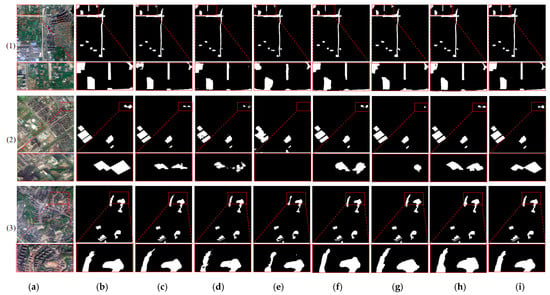
Figure 6.
Detection results of different methods on the dust source dataset HDSD-A. The second row of red boxes in each set of images is a zoomed-in effect of the first row of red boxes. (a) Image, (b) label, (c) VGG16+U-Net, (d) ResNet50+U-Net, (e) MobileNetV3+U-Net, (f) SDSC-UNet, (g) FTUNetformer, (h) FTransUNet, and (i) DSU-Net (ours).
4.4. Experimental Results on Dust Source Dataset HDSD-B
The evaluation metrics of the comparison experiments on dataset HDSD-B with different types of dust control measures are shown in Table 3. According to the analysis based on the category with dust control measures, our proposed DSU-Net improves mIoU and mprecision by 1.2% and 0.7%, respectively, compared with the baseline VGG16+U-Net. Compared to ResNet50+U-Net, our method improves mIoU by 7.9%, mprecision by 3.6%, and mrecall by 5.7%. Compared to Segformer, our method improves mIoU by 21.8%, mprecision by 14.2%, and mrecall by 13.6%. Compared to the latest FTransUNet, FTUNetformer, and SDSC-UNet, our approach improves mIoU by 0.2%, 0.7%, and 1.3%, mprecision by 0.3%, 1.2%, and 1.7%, and mrecall by 0.9%, 1.5%, and 3.0%, respectively. For the category without dust control measures, our DSU-Net improved mIoU by 1.5%, mprecision by 0.4%, and mrecall by 1.5% over the baseline VGG16+U-Net method. Comparing with ResNet50+U-Net, the proposed method improves mIoU by 10.6%, mprecision by 3.8%, and mrecall by 8.7%. Compared to Segformer, our method improves mIoU by 25.8%, mprecision by 11.2%, and mrecall by 21.7%. Compared with the latest FTransUNet, FTUNetformer, and SDSC-UNet, our method obtains different degrees of improvement in mIoU, mprecision, and mrecall, respectively. For the whole dust source dataset HDSD-B, our proposed DSU-Net method achieves 92.2% mIoU, which is 0.5~16.5% higher than the mIoU of the other methods, respectively, and 0.6~9.9% and 0.6~12.0% higher than the other methods in mprecision and mrecall, respectively. Although our mrecall is slightly lower than the baseline by 0.4% in the category with dust control measures, as a whole, the segmentation accuracy of our method is still better than other methods.

Table 3.
Segmentation results of different methods on dust source dataset HDSD-B.
The visualisation results of the experiments on dust source dataset HDSD-B are shown in Figure 7. The yellow part of the predicted image indicates the dust source with dust control measures, and the white part is the dust source without dust control measures. To identify and analyse the segmentation effect of various methods on dust sources more clearly, we overlay the segmentation results of different parting methods with the corresponding original images. The detailed parts with large differences are also labelled with red circles. As can be seen from the images in group (1), our method is closest to the effect of manually annotated labels, and the segmentation results are finer. Observing the part of construction site dust sources marked by red circles, the segmentation effects of FTransUNet, FTUNetformer, SDSC-UNet, and the baseline VGG16+U-Net are close, all of them recognise two dust sources as one dust source, and the boundary part is not clearly segmented. There are also some false detection areas in the segmentation results obtained by ResNet50+U-Net. In addition, Segformer’s segmentation results exhibit the misdetection of dust source patches and poor detection in the boundary part of the dust source. As can be seen from the images in group (2), for the dust sources with dust control measures, our method is comparable to the baseline VGG16+U-Net and FTransUNet in terms of recognition. Additionally, the Segformer method predicts the most blurred boundaries of dust source patches with dust suppression measures. Similarly, observing the portion marked by red circles, the VGG16+U-Net method falsely detects a dust source with dust control measures. In contrast, ResNet50+U-Net, SDSC-UNet, and FTUNetformer do not detect the dust source here. Moreover, ResNet50+U-Net recognises three dust sources as one dust source when identifying the dust source without dust control measures in the middle, blurring the information of their respective boundaries. The dust source area of the image in group (3) is denser, and the ResNet50+U-Net, Segformer, and SDSC-UNet methods exhibit misdetection. As can be seen from the parts marked by red circles, our method recognises the boundaries of two dust sources, while all other methods recognise them as one dust source. In group (4), for the part of dust sources with dust control measures in yellow colour, the detection effect of various methods is similar. In the part of the dust source without dust control measures, our method is the most effective in recognising the dust source.
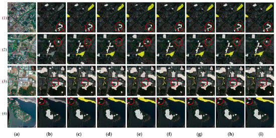
Figure 7.
Detection results of different methods on dust source dataset HDSD-B, which distinguishes dust control measures. The detection results of various methods overlaid with the original images are presented. The red circles mark the detailed areas with large differences in the segmentation results of the different methods. (a) Image, (b) label, (c) VGG16+U-Net, (d) ResNet50+U-Net, (e) Segformer, (f) SDSC-UNet, (g) FTUNetformer, (h) FTransUNet, and (i) DSU-Net (ours).
4.5. Ablation Experiment
4.5.1. Analysis of the Loss Function
The ablation experiment is conducted for the analysis of the impact of the loss function on the experiments. When using the standard Dice Loss + Focal Loss as the training loss function for the network, it becomes evident that the loss shows greater oscillations, and the convergence of accuracy is not optimal. After we incorporate Activate Boundary Loss on this basis, the network training loss and validation loss curves obtained are smoother, and the convergence achieves higher accuracy, as shown in Figure 8. The loss function has been validated on both dust source dataset HDSD-A and HDSD-B, respectively. Table 4 shows the results of the ablation experiments, with black bolding indicating the optimal results. The experimental results show that the segmentation accuracy obtained after incorporating the Active Boundary Loss function is high.
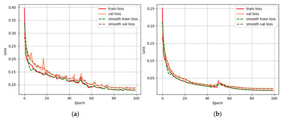
Figure 8.
(a) Loss function plot for the common Dice Loss + Focal Loss combination. (b) Loss function plot incorporating Activate Boundary Loss.

Table 4.
Segmentation effects in DSU-Net using different loss functions on two datasets.
In addition, we perform a sensitivity analysis of the hyperparameters of the loss function on the HDSD-A dataset. Among them, Dice Loss directly focuses on the global segmentation accuracy. Based on experience, we directly set λ1 to 1.0. Then we select different λ2 and λ3 for separate sensitivity validation of Focal Loss and Activate Boundary Loss. Figure 9a shows the effect of DSU-Net taking different values of λ2 on mIoU. A larger λ2 leads to a decrease in the global segmentation ability, and a smaller λ2 reduces the recognition ability to handle small targets. As can be seen from Figure 9a, when λ2 ≥ 2.0, the performance of the model decreases significantly. And when λ2 ∈ [0.1, 1.0], the performance of the model shows an increasing trend. Therefore, for Focal Loss, we choose λ2 as 1.0. Also, Figure 9b demonstrates the effect of DSU-Net taking different values of λ3 on mIoU. A larger λ3 will overemphasise the boundaries and ignore the large non-boundary regions. While a smaller λ3 leads to less effective boundary segmentation. Observing Figure 9b, the performance of the model is increasing when λ3 ∈ [0.01, 0.1] and decreasing when λ3 ∈ [0.1, 1.0]. Therefore, for Activate Boundary Loss, we choose λ3 to be 0.1.
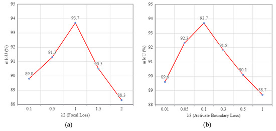
Figure 9.
(a) Hyperparametric analysis of Focal Loss. (b) Hyperparametric analysis of Activate Boundary Loss.
4.5.2. Analysis of Model Efficiency
We use floating point operations (FLOPs) and the number of model parameters (Params) to comparatively evaluate the efficiency of different models. FLOPs measure the computational complexity of the model’s reasoning, which is in units of 109 (G). Params measures the storage overhead of the model, which is in units of 106 (M). To ensure fairness, we uniformly use input images of size 3 × 256 × 256 for the computation of FLOPs and Params. The efficiency metrics of all models are shown in Table 5. It can be seen that the overall computational complexity of MobilenetV3+U-Net is optimal. Compared with the baseline VGG16+U-Net, our DS-UNet does not increase the model complexity additionally and achieves better dust source segmentation results. In addition, our DS-UNet has lower FLOPs and Params than the latest FTUNetformer. Compared with other more lightweight models, our DS-UNet shows good segmentation performance with a slight increase in model complexity.

Table 5.
Efficiency of various models.
4.5.3. Analysis of the Attention Module
We validate the attentional modules for ablation, and to maintain the unique variable principle, we use VGG16+U-Net as the base network, denoted as Base, and then we adjust the type and location of the attentional modules for comparison. Here, Base+SA-E: the base network adds the shuffle attention module located at the encoder. Base+SA-D: the base network adds the shuffle attention module located at the decoder. Base+SA-C: the base network adds the shuffle attention module located at the jump junction, i.e., our method. Base+CBAM: the base network adds the CBAM module located at the jump junction, where CBAM is introduced for a more comprehensive comparison. All experiments in this section are performed on the HDSD-A dataset, and the specific metrics are shown in Table 6.

Table 6.
Comparison of the effects of the Attention Module.
From Base+SA-E and Base+SA-D, it can be seen that by adding the shuffle attention module at the encoder or decoder location, the model is slightly less effective in segmenting the dust source. On the contrary, adding the shuffle attention module at the jump connection obtained the best segmentation results. On the HDSD-A dataset, the mIoU, mprecision and mrecall of Base+SA-C are 1.7%, 2.0% and 1.5% higher than those of Base+CBAM, respectively. Overall, Base+SA-C is the best combination.
4.6. Application Analysis in Different Cities
To further validate the feasibility of our method to detect dust sources in urban areas, we selected the remote sensing image of Yicheng City, Hubei Province, from Jilin 1 satellite in April 2023 as a new test area. Notably, the Yicheng city in Hubei Province is not seen by the model here. Taking the surface features reflected on the remote sensing images as the important interpretation basis, we visually interpreted the remote sensing images of Yicheng City and outlined and monitored 265 dust source patches with an area of more than 800 square meters, with a total area of about 8,389,961.7 square meters, and counted the number and area of dust sources in each town, as shown in Table 7.

Table 7.
Statistics on the number and area of dust sources in each town of Yicheng City.
Then, we cut the remote sensing images of Yicheng city into 849 images of 1600 × 1600 size in total and feed them into the network to predict directly and obtain the mask map. After that, the geographic information corresponding to the original image is assigned to the mask map predicted by the model, and the 849 mask maps are concatenated to form the complete Yicheng city. Due to the practical application, the decoded dust source patches are not made into labels. Therefore, we directly calculate the indexes of precision and recall by detecting the number of dust source patches. Specifically, we first use the ArcGIS tool to convert the Yicheng dust source mask map with geographic information into a shpfile file and calculate the area of each predicted patch. According to the actual detection needs, after deleting the predicted patches with an area less than 100 square meters, a total of 565 predicted patches were finally obtained, as shown in Figure 10. Then, the intersection of predicted patches and interpreted patches is calculated to obtain 438 dust source patches.
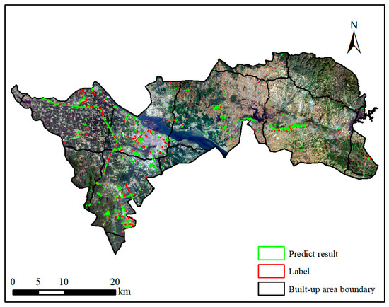
Figure 10.
Predicted results for Yicheng City. The green box shows the results predicted by the model and the red box shows the results of the interpretation.
From Figure 10, there are multiple prediction results indicating the same target, which we transformed into uniquely identifying one target, and the intersection result after deletion is 195, i.e., the true examples TP = 195. According to the definition of false positive examples FP and false negative examples FN, it is known that FP = 565 − 438 = 127 and FN = 265 − 195 = 70.
From this, the precision rate can be obtained as shown in Equation (15):
and the recall rate is shown in Equation (16):
In order to verify the generalisation ability of DSU-Net more comprehensively, we choose two districts that are geographically different from Hubei Province to conduct the experiment. One is Wuda District of Wuhai City, which is in the southwest of Inner Mongolia Autonomous Region and in the upper reaches of the Yellow River. The geography of the area is dominated by desert and Gobi, and the terrain is relatively flat, but there are some low hills and mountains around. The other is the Tieshangang District of Beihai City, which is in the southern part of the Guangxi Zhuang Autonomous Region, adjacent to the coast of the Beibu Gulf. The topography of the district is dominated by coastal plains with relatively flat terrain and large areas of mudflats and wetlands along the coast. Among them, Wuda District uses Gaofen-1 satellite remote sensing images from January 2022. Through visual interpretation, we monitored 59 dust source patches with a total area of about 39,456,802.1 square meters. Tieshan Harbor District uses Sentinel-2A satellite remote sensing images from January 2023. We monitored and obtained 75 dust source patches with a total area of about 10,483,334.2 square meters. Consistent with the validation of the method in Yicheng City, Hubei Province, the prediction result map for Wuda District is shown in Figure 11, and the prediction result map for Tieshangang District is shown in Figure 12.
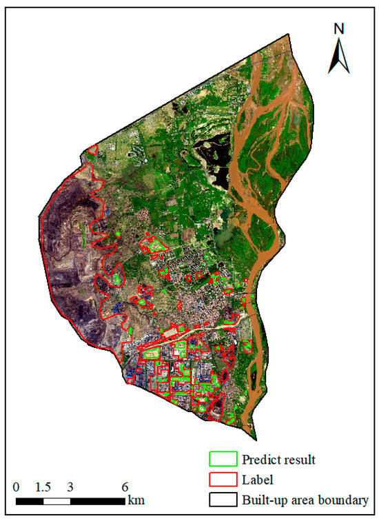
Figure 11.
Predicted results for Wuda District. The green box shows the results predicted by the model and the red box shows the results of the interpretation.
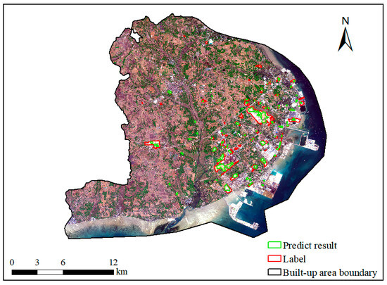
Figure 12.
Predicted results for Tieshangang District. The green box shows the results predicted by the model and the red box shows the results of the interpretation.
As can be observed from Figure 11, due to the unique geomorphology of Wuda District, it has a special type of dust source, i.e., bare mountain. For the bare mountain dust source, our method is not effective in recognising it. However, for other types of dust sources, DSU-Net is effective in recognising them. Statistically, DSU-Net correctly identifies 43 dust sources, i.e., true cases TP = 43. In addition, there are 27 falsely detected dust sources, i.e., false positive cases FP = 27, and the false negative case FN is the number of true dust sources minus true cases, i.e., FN = 59 − 43 = 16. From this, we can calculate the precision rate, which is shown in Equation (17):
and the recall rate is shown in Equation (18):
As can be seen from Figure 12, the overall recognition effect is good, and some slight misdetection cases occur. Statistically, DSU-Net correctly recognises 59 dust sources, i.e., true cases TP = 59, while there are 25 falsely detected dust sources, i.e., false positive cases FP = 25. then, we calculate to obtain the false negative cases FN = 75 − 59 = 16. Similarly, we calculate to obtain the precision rate as shown in Equation (19):
and the recall rate is shown in Equation (20):
After the above analysis, it is verified that our method can be applied to the detection of dust sources in real urban scenarios, and it can provide some technical support for related stakeholders.
5. Discussion
We further conducted a detailed analysis of the dust source detection results, classifying the results into four categories. The “Good Recognition” category indicates that the prediction results closely match the interpretation results, reflecting a high recognition accuracy. The “False Recognition” category refers to instances where the model incorrectly identifies a situation. The “Missed Recognition” category indicates cases where the model omits the recognition. The “Correct Recognition” category instances where the model successfully identified dust sources that were not indicated in the interpretation results. Figure 13 shows the representative visualisation results of the four cases. The model is more effective in recognising dust sources for bare ground type and building construction type. However, the model is prone to misidentify plants or concrete floors as dust sources. This is since these plants are located on bare ground and the vehicles are stacked in an unorganised manner, which is like the characteristics of construction sites. The characteristics of concrete floors are close to those of dust sources with dust control measures, which makes it easy to misidentify them. Similarly, over-exposed dust source patches in the image are prone to misdetection because these dust source features are blurred, which makes the model unable to recognise them accurately. It is worth mentioning that the model we trained using the constructed dataset can identify some dust sources that were not indicated in the interpretation results.
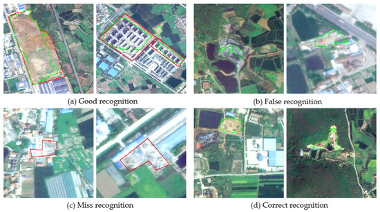
Figure 13.
Visual analysis of the detection results of dust sources. The green box shows the results predicted by the model and the red box shows the results of the interpretation.
6. Conclusions
In this paper, we first created two datasets of dust source images using high-resolution remote sensing images from the Jilin-1 satellite for three representative cities of Jingmen City, Jingzhou City, and Yichang City in Hubei Province. These two datasets were used for the segmentation of dust sources in high-resolution remote sensing images, of which dataset B was specifically used for distinguishing dust control measures. In order to accurately detect the dust sources from remote sensing images, we proposed a new DSU-Net segmentation network, which replaced the backbone extraction network on the basis of U-Net and introduces the SA mechanism into the jump branch part of U-Net. In addition, we incorporated Activate Boundary Loss into the loss function, which can adaptively adjust the loss weights according to the prediction of the boundary pixels and impose a greater penalty on those boundary pixels with inaccurate prediction. Comparisons were made with VGG16+U-Net, ResNet50+U-Net, and MobileNetV3+U-Net using our created dataset HDSD-A, and with VGG16+U-Net, ResNet50+U-Net, and Segformer using our created dataset HDSD-B. Both sets of experiments demonstrated the effectiveness of our proposed method for the automatic detection of dust sources. Meanwhile, we also conducted a generalisability validation in Yicheng City, Hubei Province, Wuda District of Wuhai City, Tieshangang District of Beihai City, and the results showed that the method in this paper has some practical application value. In future work, our research will focus on expanding and enriching the dust source datasets, incorporating multi-scale identification techniques, and enhancing the detection method to achieve higher segmentation accuracy.
Author Contributions
Conceptualisation, Z.W. and L.B.; methodology, Z.W., L.B. and X.H.; software, X.H.; validation, X.H.; formal analysis, X.H.; investigation, L.B., Z.W. and X.H.; resources, L.B., Z.W. and X.H.; data curation, Z.W. and X.H.; writing—original draft preparation, Z.W., L.B. and X.H.; writing—review and editing, L.B., Z.W., X.H., M.F., Y.C. and L.C.; visualisation, X.H.; supervision, Z.W. and L.B.; project administration, L.C.; funding acquisition, Z.W. and L.C. All authors have read and agreed to the published version of the manuscript.
Funding
This work was supported in part by TUOHAI special project 2020 from Bohai Rim Energy Research Institute of Northeast Petroleum University under Grant HBHZX202002, Heilongjiang Province Higher Education Teaching Reform Project under Grant SJGY20200125 and National Key Research and Development Program of China under Grant 2022YFC330160204.
Data Availability Statement
Data available on request from the authors.
Conflicts of Interest
The authors declare no conflict of interest.
References
- Feng, Y.; Ning, M.; Lei, Y.; Sun, Y.; Liu, W.; Wang, J. Defending blue sky in China: Effectiveness of the “Air Pollution Prevention and Control Action Plan” on air quality improvements from 2013 to 2017. J. Environ. Manag. 2019, 252, 109603. [Google Scholar] [CrossRef] [PubMed]
- Qin, J.X.; Zhu, K.Y.; Wu, T.; Shen, H.Q. Study on spatial and temporal characteristics of construction dust and soil dust pollution sources in urban areas of Changsha. Environ. Monit. China 2020, 36, 69–79. [Google Scholar]
- Song, L.L.; Li, T.K.; Bi, X.H.; Wang, X.H.; Zhang, W.H.; Zhang, Y.F.; Wu, J.; Feng, Y.C. Construction and dynamic method of soil fugitive dust emission inventory with high spatial resolution in Beijing-Tianjin-Hebei Region. Res. Environ. Sci. 2021, 34, 1771–1781. [Google Scholar]
- Ministry of Environmental Protection. Technical Guide for the Compilation of Emission Inventory for Particulate Matter from Dust Sources (Trial Implementation) [FP/OL]. Available online: http://www.mee.gov.cn/gkml/hbb/bgg/201501/W020-150107594588131490.pdf (accessed on 31 December 2014).
- Jiang, S.; Ji, X.; Li, X.; Wang, T.; Tao, J. Method Study and Result Analysis on Remote Sensing Monitoring of Fugitive Dust from Construction Sites and Bare Area in Jiangsu Province. Environ. Monit. Forewarn. 2022, 14, 12–18. [Google Scholar]
- Kahraman, M.M.; Erkayaoglu, M. A Data-Driven Approach to Control Fugitive Dust in Mine Operations. Min. Metall. Explor. 2021, 38, 549–558. [Google Scholar] [CrossRef]
- Zhang, Q.; Wang, R.; Shen, Y.; Zhan, L.; Xu, Z. Characteristics of unorganized emissions of microplastics from road fugitive dust in urban mining bases. Sci. Total Environ. 2022, 827, 154355. [Google Scholar] [CrossRef]
- Kolesar, K.R.; Schaaf, M.D.; Bannister, J.W.; Schreuder, M.D.; Heilmann, M.H. Characterization of potential fugitive dust emissions within the Keeler Dunes, an inland dune field in the Owens Valley, California, United States. Aeolian Res. 2022, 54, 100765. [Google Scholar] [CrossRef]
- Zhao, Y.; Wang, Y.; Qiu, F. Prediction method of dust pollutant diffusion range in building demolition based on Euclidean distance transformation. Int. J. Environ. Technol. Manag. 2023, 26, 250–262. [Google Scholar] [CrossRef]
- Rayegani, B.; Barati, S.; Goshtasb, H.; Gachpaz, S.; Ramezani, J.; Sarkheil, H. Sand and dust storm sources identification: A remote sensing approach. Ecol. Indic. 2020, 112, 106099. [Google Scholar] [CrossRef]
- Yu, H.; Zahidi, I. Environmental hazards posed by mine dust, and monitoring method of mine dust pollution using remote sensing technologies: An overview. Sci. Total Environ. 2023, 864, 161135. [Google Scholar] [CrossRef]
- Xu, Z.; Han, Y.; Ren, D. Coupling Phenomenon Between Fugitive Dust and High-Temperature Tail Gas: A Thermal Infrared Signature Study. J. Therm. Sci. Eng. Appl. 2023, 15, 031011. [Google Scholar] [CrossRef]
- Ma, Z.; Xia, M.; Weng, L.; Lin, H. Local Feature Search Network for Building and Water Segmentation of Remote Sensing Image. Sustainability 2023, 15, 3034. [Google Scholar] [CrossRef]
- Dai, X.; Xia, M.; Weng, L.; Hu, K.; Lin, H.; Qian, M. Multiscale Location Attention Network for Building and Water Segmentation of Remote Sensing Image. IEEE Trans. Geosci. Remote Sens. 2023, 61, 5609519. [Google Scholar] [CrossRef]
- Yuan, G.; Li, J.; Liu, X.; Yang, Z. Weakly supervised road network extraction for remote sensing image based scribble annotation and adversarial learning. J. King Saud Univ.—Comput. Inf. Sci. 2022, 34, 7184–7199. [Google Scholar] [CrossRef]
- Li, L.; Lu, N.; Jiang, H.; Qin, J. Impact of Deep Convolutional Neural Network Structure on Photovoltaic Array Extraction from High Spatial Resolution Remote Sensing Images. Remote Sens. 2023, 15, 4554. [Google Scholar] [CrossRef]
- Shi, K.; Bai, L.; Wang, Z.; Tong, X.; Mulvenna, M.D.; Bond, R.R. Photovoltaic Installations Change Detection from Remote Sensing Images Using Deep Learning. In Proceedings of the IGARSS 2022—2022 IEEE International Geoscience and Remote Sensing Symposium, Kuala Lumpur, Malaysia, 17–22 July 2022; pp. 3231–3234. [Google Scholar]
- Xu, S.; Zhang, H.; He, X.; Cao, X.; Hu, J. Oil Tank Detection with Improved EfficientDet Model. IEEE Geosci. Remote Sens. Lett. 2022, 19, 1–5. [Google Scholar] [CrossRef]
- Zhu, M.; Wang, Z.; Bai, L.; Zhang, J.; Tao, J.; Chen, L. Detection of industrial storage tanks at the city-level from optical satellite remote sensing images. In Proceedings of the Image and Signal Processing for Remote Sensing XXVII, Online, 13–17 September 2021; SPIE: Bellingham, WA, USA, 2021; pp. 266–272. [Google Scholar]
- Zhang, Y.; Bai, L.; Wang, Z.; Fan, M.; Jurek-Loughrey, A.; Zhang, Y.; Zhang, Y.; Zhao, M.; Chen, L. Oil Well Detection under Occlusion in Remote Sensing Images Using the Improved YOLOv5 Model. Remote Sens. 2023, 15, 5788. [Google Scholar] [CrossRef]
- Wang, Z.; Bai, L.; Song, G.; Zhang, Y.; Zhu, M.; Zhao, M.; Chen, L.; Wang, M. Optimized faster R-CNN for oil wells detection from high-resolution remote sensing images. Int. J. Remote Sens. 2023, 44, 6897–6928. [Google Scholar] [CrossRef]
- Chang, H.; Bai, L.; Wang, Z.; Wang, M.; Zhang, Y.; Tao, J.; Chen, L. Detection of over-ground petroleum and gas pipelines from optical remote sensing images. In Proceedings of the Image and Signal Processing for Remote Sensing XXIX, Amsterdam, The Netherlands, 4–5 September 2023; SPIE: Bellingham, WA, USA, 2023; Volume 12733, pp. 315–321. [Google Scholar]
- Wu, H.; Dong, H.; Wang, Z.; Bai, L.; Huo, F.; Tao, J.; Chen, L. Semantic segmentation of oil well sites using Sentinel-2 imagery. In Proceedings of the IGARSS 2023—2023 IEEE International Geoscience and Remote Sensing Symposium, Pasadena, CA, USA, 16–21 July 2023; IEEE: New York, NY, USA, 2023; pp. 6901–6904. [Google Scholar]
- Yu, C.; Hu, Z.; Li, R.; Xia, X.; Zhao, Y.; Fan, X.; Bai, Y. Segmentation and density statistics of mariculture cages from remote sensing images using mask R-CNN. Inf. Process. Agric. 2022, 9, 417–430. [Google Scholar] [CrossRef]
- Wang, J.; Fan, J.; Wang, J. MDOAU-Net: A Lightweight and Robust Deep Learning Model for SAR Image Segmentation in Aquaculture Raft Monitoring. IEEE Geosci. Remote Sens. Lett. 2022, 19, 1–5. [Google Scholar] [CrossRef]
- Sun, Z.; Zhou, W.; Ding, C.; Xia, M. Multi-Resolution Transformer Network for Building and Road Segmentation of Remote Sensing Image. ISPRS Int. J. Geo-Inf. 2022, 11, 165. [Google Scholar] [CrossRef]
- Zeng, Y.; Guo, Y.; Li, J. Recognition and extraction of high-resolution satellite remote sensing image buildings based on deep learning. Neural Comput. Appl. 2022, 34, 2691–2706. [Google Scholar] [CrossRef]
- Zhou, Y.; Chen, Z.; Wang, B.; Li, S.; Liu, H.; Xu, D.; Ma, C. BOMSC-Net: Boundary Optimization and Multi-Scale Context Awareness Based Building Extraction from High-Resolution Remote Sensing Imagery. IEEE Trans. Geosci. Remote Sens. 2022, 60, 1–17. [Google Scholar] [CrossRef]
- Fan, X.; Yan, C.; Fan, J.; Wang, N. Improved U-Net Remote Sensing Classification Algorithm Fusing Attention and Multiscale Features. Remote Sens. 2022, 14, 3591. [Google Scholar] [CrossRef]
- Li, S.; Liao, C.; Ding, Y.; Hu, H.; Jia, Y.; Chen, M.; Xu, B.; Ge, X.; Liu, T.; Wu, D. Cascaded Residual Attention Enhanced Road Extraction from Remote Sensing Images. ISPRS Int. J. Geo-Inf. 2022, 11, 9. [Google Scholar] [CrossRef]
- Li, R.; Wang, L.; Zhang, C.; Duan, C.; Zheng, S. A2-FPN for semantic segmentation of fine-resolution remotely sensed images. Int. J. Remote Sens. 2022, 43, 1131–1155. [Google Scholar] [CrossRef]
- Wang, L.; Li, R.; Zhang, C.; Fang, S.; Duan, C.; Meng, X.; Atkinson, P.M. UNetFormer: A UNet-like transformer for efficient semantic segmentation of remote sensing urban scene imagery. ISPRS J. Photogramm. Remote Sens. 2022, 190, 196–214. [Google Scholar] [CrossRef]
- Sun, Y.; Bi, F.; Gao, Y.; Chen, L.; Feng, S. A Multi-Attention UNet for Semantic Segmentation in Remote Sensing Images. Symmetry 2022, 14, 906. [Google Scholar] [CrossRef]
- Yuan, M.; Ren, D.; Feng, Q.; Wang, Z.; Dong, Y.; Lu, F.; Wu, X. MCAFNet: A Multiscale Channel Attention Fusion Network for Semantic Segmentation of Remote Sensing Images. Remote Sens. 2023, 15, 361. [Google Scholar] [CrossRef]
- Wang, Z.; Wang, J.; Yang, K.; Wang, L.; Su, F.; Chen, X. Semantic segmentation of high-resolution remote sensing images based on a class feature attention mechanism fused with Deeplabv3+. Comput. Geosci. 2022, 158, 104969. [Google Scholar] [CrossRef]
- Wu, S.; Liu, Y.; Liu, S.; Wang, D.; Yu, L.; Ren, Y. Change detection enhanced by spatial-temporal association for bare soil land using remote sensing images. In IEEE Journal of Selected Topics in Applied Earth Observations and Remote Sensing; IEEE: New York, NY, USA, 2023. [Google Scholar]
- He, X.; Wang, Z.; Bai, L.; Wang, M.; Fan, M. Detection of urban fugitive dust emission sources from optical satellite remote sensing images. In Remote Sensing Technologies and Applications in Urban Environments VIII; SPIE: Bellingham, WA, USA, 2023; pp. 73–79. [Google Scholar]
- de Silva, A.; Ranasinghe, R.; Sounthararajah, A.; Haghighi, H.; Kodikara, J. Beyond Conventional Monitoring: A Semantic Segmentation Approach to Quantifying Traffic-Induced Dust on Unsealed Roads. Sensors 2024, 24, 510. [Google Scholar] [CrossRef] [PubMed]
- Liu, J.; Feng, Q.; Wang, Y.; Batsaikhan, B.; Gong, J.; Li, Y.; Liu, C.; Ma, Y. Urban green plastic cover mapping based on VHR remote sensing images and a deep semi-supervised learning framework. ISPRS Int. J. Geo-Inf. 2020, 9, 527. [Google Scholar] [CrossRef]
- Cao, Y.; Huang, X. A coarse-to-fine weakly supervised learning method for green plastic cover segmentation using high-resolution remote sensing images. ISPRS J. Photogramm. Remote Sens. 2022, 188, 157–176. [Google Scholar] [CrossRef]
- Guo, W.; Yang, G.; Li, G.; Ruan, L.; Liu, K.; Li, Q. Remote sensing identification of green plastic cover in urban built-up areas. Environ. Sci. Pollut. Res. 2023, 30, 37055–37075. [Google Scholar] [CrossRef]
- Zhang, Q.-L.; Yang, Y.-B. SA-Net: Shuffle Attention for Deep Convolutional Neural Networks. In Proceedings of the ICASSP 2021—2021 IEEE International Conference on Acoustics, Speech and Signal Processing (ICASSP), Toronto, ON, Canada, 6–11 June 2021; pp. 2235–2239. [Google Scholar]
- Wang, C.; Zhang, Y.; Cui, M.; Ren, P.; Yang, Y.; Xie, X.; Hua, X.S.; Bao, H.; Xu, W. Active boundary loss for semantic segmentation. Proc. AAAI Conf. Artif. Intell. 2022, 36, 2397–2405. [Google Scholar] [CrossRef]
- Ronneberger, O.; Fischer, P.; Brox, T. U-Net: Convolutional Networks for Biomedical Image Segmentation. In Medical Image Computing and Computer-Assisted Intervention—MICCAI 2015; Navab, N., Hornegger, J., Wells, W.M., Frangi, A.F., Eds.; Lecture Notes in Computer Science; Springer International Publishing: Cham, Switzerland, 2015; Volume 9351, pp. 234–241. [Google Scholar]
- Simonyan, K.; Zisserman, A. Very deep convolutional networks for large-scale image recognition. arXiv 2014, arXiv:1409.1556. [Google Scholar]
- Hu, J.; Shen, L.; Sun, G. Squeeze-and-Excitation Networks. In Proceedings of the IEEE Conference on Computer Vision and Pattern Recognition, Salt Lake City, UT, USA, 18–23 June 2018; pp. 7132–7141. [Google Scholar]
- Wu, Y.; He, K. Group Normalization. In Proceedings of the European Conference on Computer Vision (ECCV), Munich, Germany, 8–14 September 2018; pp. 3–19. [Google Scholar]
- Li, X.; Sun, X.; Meng, Y.; Liang, J.; Wu, F.; Li, J. Dice loss for data-imbalanced NLP tasks. arXiv 2019, arXiv:1911.02855. [Google Scholar]
- Yeung, M.; Sala, E.; Schönlieb, C.-B.; Rundo, L. Unified Focal loss: Generalising Dice and cross entropy-based losses to handle class imbalanced medical image segmentation. Comput. Med. Imaging Graph. 2022, 95, 102026. [Google Scholar] [CrossRef]
- Xie, E.; Wang, W.; Yu, Z.; Anandkumar, A.; Alvarez, J.M.; Luo, P. SegFormer: Simple and efficient design for semantic segmentation with transformers. Adv. Neural Inf. Process. Syst. 2021, 34, 12077–12090. [Google Scholar]
- Zhang, R.; Zhang, Q.; Zhang, G. SDSC-UNet: Dual skip connection ViT-based U-shaped model for building extraction. IEEE Geosci. Remote Sens. Lett. 2023, 20, 6005005. [Google Scholar] [CrossRef]
- Ma, X.; Wu, Q.; Zhao, X.; Zhang, X.; Pun, M.O.; Huang, B. Sam-assisted remote sensing imagery semantic segmentation with object and boundary constraints. In IEEE Transactions on Geoscience and Remote Sensing; IEEE: New York, NY, USA, 2024. [Google Scholar]
- Ma, X.; Zhang, X.; Pun, M.O.; Liu, M. A multilevel multimodal fusion transformer for remote sensing semantic segmentation. In IEEE Transactions on Geoscience and Remote Sensing; IEEE: New York, NY, USA, 2024. [Google Scholar]
Disclaimer/Publisher’s Note: The statements, opinions and data contained in all publications are solely those of the individual author(s) and contributor(s) and not of MDPI and/or the editor(s). MDPI and/or the editor(s) disclaim responsibility for any injury to people or property resulting from any ideas, methods, instructions or products referred to in the content. |
© 2024 by the authors. Licensee MDPI, Basel, Switzerland. This article is an open access article distributed under the terms and conditions of the Creative Commons Attribution (CC BY) license (https://creativecommons.org/licenses/by/4.0/).