Automated Hyperspectral Feature Selection and Classification of Wildlife Using Uncrewed Aerial Vehicles

Abstract

Timely and accurate detection and estimation of animal abundance is an important part of wildlife management. This is particularly true for invasive species where cost-effective tools are needed to enable landscape-scale surveillance and management responses, especially when targeting low-density populations residing in dense vegetation and under canopies. This research focused on investigating the feasibility and practicality of using uncrewed aerial systems (UAS) and hyperspectral imagery (HSI) to classify animals in the wild on a spectral—rather than spatial—basis, in the hopes of developing methods to accurately classify animal targets even when their form may be significantly obscured. We collected HSI of four species of large mammals reported as invasive species on islands: cow (Bos taurus), horse (Equus caballus), deer (Odocoileus virginianus), and goat (Capra hircus) from a small UAS. Our objectives of this study were to (a) create a hyperspectral library of the four mammal species, (b) study the efficacy of HSI for animal classification by only using the spectral information via statistical separation, (c) study the efficacy of sequential and deep learning neural networks to classify the HSI pixels, (d) simulate five-band multispectral data from HSI and study its effectiveness for automated supervised classification, and (e) assess the ability of using HSI for invasive wildlife detection. Image classification models using sequential neural networks and one-dimensional convolutional neural networks were developed and tested. The results showed that the information from HSI derived using dimensionality reduction techniques were sufficient to classify the four species with class F1 scores all above 0.85. The performances of some classifiers were capable of reaching an overall accuracy over 98%and class F1 scores above 0.75, thus using only spectra to classify animals to species from existing sensors is feasible. This study discovered various challenges associated with the use of HSI for animal detection, particularly intra-class and seasonal variations in spectral reflectance and the practicalities of collecting and analyzing HSI data over large meaningful areas within an operational context. To make the use of spectral data a practical tool for wildlife and invasive animal management, further research into spectral profiles under a variety of real-world conditions, optimization of sensor spectra selection, and the development of on-board real-time analytics are needed.

1. Introduction

Invasive animals are one of the leading threats to island ecosystems and the animal and human communities that depend on them [1]. Eliminating invasive mammals from islands is a proven tool for kickstarting the recovery of island species and habitats. This recovery has been increasingly linked to mitigating and adapting to climate change, improved human wellbeing, and strengthening land–sea connections and coastal ecosystems [2,3,4,5,6]. The eradication of invasive species on islands has resulted in significant progress toward reducing global extinctions, and were specifically called out as priority sites for conservation action in the Kunming–Montreal Global Biodiversity Framework [7]. Global trends in invasive species eradication on islands is increasing, with practitioners attempting increasingly larger and more complex projects [2]. With this increasing trend comes the need for new tools and methodologies to improve the cost-efficiency of island eradications to meet conservation needs [8,9,10].

An estimated one-third or more of invasive mammal eradication projects costs are spent detecting and removing the target individuals from a system [11,12]. Moreover, these costs exponentially increase per animal as the population dwindles to the last few individuals, particularly when removing invasive species on islands using progressive removal strategies [13]. As such, significant investment and research spent on identifying new methods to detect invasive mammals quickly and accurately within vast landscapes is critical to improve management response and operational decision making [14]. Specifically, near-real time detection methods are needed to improve confidence in invasive species eradication success sooner and cost-effectively deploy resources in response to detections of animals at low densities.

Most currently available visual detection methods deployed for invasive species management use visible or thermal imagery to detect or classify species. These robust methods primarily rely on shape-based, spatial characteristics to classify and distinguish between species and backgrounds [15]. Where species have similar spatial characteristics, shape-based approaches can have difficulty in accurately distinguishing between species, requiring manual review of detections after the fact, changes in flight parameters to increase resolution, or the use of video to distinguish between species based on movement. Each of these responses can lead to delayed management actions and can limit the effectiveness of aerial-based detection methods to comprehensively survey a management area. This issue is particularly acute in tropical island environments, where lush vegetation and contiguous canopies likely obscure large portions of a targeted animal’s form.

Further, developing accurate models for target species of interest requires extensive training datasets, and these models generally experience a significant loss in classification accuracy when applied to new, untrained locations and are not generalizable across a broad set of diverse ecosystems [16,17]. Invasive species managers generally intend to remove populations within a short time period with significant effort spent in an initial knockdown of the population in a single breeding season. Thus, the images and personnel resources needed for data labeling and model training are often not available until the project is already in the key stages of low population densities when accurate models are needed most. Consequently, the use of detection models for project-based, island invasive species management is particularly limited. These are often short discrete actions (<5 years) conducted in a globally diverse set of ecosystems, compared to on-going control efforts in continental systems, where there may be a higher per-organization return on investment from model development.

Given these constraints, detection efforts for island invasive species management typically require significant manual effort or rely on general object detectors to identify species of interest that need to be reviewed by experts to classify to species levels. This can limit the timeliness of operational decision making or the ability of managers to deploy and maintain a comprehensive island-wide surveillance methodology necessary to quickly declare or evaluate eradication success. Thus, island invasive species eradication will benefit from novel, highly accurate methods for detecting target species of interest from relatively low sample sizes, i.e., reflectance—not shape—based classification models, and where methods that are more broadly applicable across ecosystem backgrounds and require less bespoke development and optimization for use in a new location, are utilized.

One of the prerequisites for successful management of wildlife is an accurate assessment of the population [18]. Previous methods of obtaining these population estimates include using crewed aerial vehicles, crewed ground vehicles, satellites, and more recently, uncrewed aerial vehicles (UAS) [18,19,20]. While detection and counting methods have shown to be useful and even improved upon by using automatic detection algorithms, these methods mainly use spatial characteristics from recorded imagery [19,21,22,23]. Most of these workflows use visible, thermal, or some combination of the two types of imagery [15,24].

While visible, infrared, and thermal imagery have their use in surveying landscapes and classifying the animals within, their reliance on shape-based detection models do have some significant limitations, such as canopy occlusion, and a limited number of spectral channels. Hyperspectral imagery from remote sensing platforms has the potential to alleviate these limitations. Hyperspectral sensors capture the reflected electromagnetic energy from the target over hundreds to thousands of narrow near-contiguous spectral bands. The spectral bands contain rich information about the target’s physical and chemical properties since the light reflectance at different wavelengths correspond to unique atomic and molecular structures of the target. While hyperspectral sensors are passive and cannot penetrate mediums, the large amount of information from a small spatial sample may be enough to positively identify the scene.

Hyperspectral sensors are widely used in fields such as mining [25], forestry [26], ecology [9], and agriculture [27]. With recent developments, machine learning algorithms have become a vital tool to understand and model rich information captured by hyperspectral sensors. Machine learning models used on hyperspectral data have evolved over the years, starting from statistical machine learning, such as Bayesian to kernel based methods such as support vector machines, to deep learning neural networks [28,29,30,31]. There have been a few studies looking at hyperspectral spectroscopy to differentiate between species of fish, mammals, and artificial structures [32,33,34,35,36,37,38,39].

Past research has indicated that mammals are readily discernable from vegetation in the visible and NIR regions, that there is significant intraspecies variability in the VNIR among individuals based on their pelage and pigmentation, and that there are spectra in the SWIR likely attributed to the structural proteins that make up the animals’ hair that could be used to accurately distinguish between different mammal species [34,35,39]. Collectively, this small body of evidence points toward a promising potential for hyperspectral animal detection with an emphasis on high-resolution assessments of spectra and the use of data processing techniques to identify subsets of spectra that could be used to accurately identify animals and deployed in a purpose-built lower-cost, high-spatial resolution aerial sensor.

This study advances upon existing research to investigate the efficacy of using UAS remotely sensed hyperspectral imagery (HSI) to classify large mammals that commonly occur as invasive species on islands, with the goal being to accurately identify these large mammals without spatial characteristics, i.e., shape, but instead through only using their spectral signature. Few studies have investigated the utility of spectra beyond the visible range to detect mammal species and no published studies have investigated the utility of high-resolution (<5 cm) HSI to accurately distinguish between mammal species nor applied recent advances in HSI feature selection and deep learning to identify priority spectra for mammal detection. Thus, this study marks the first attempt to apply high-resolution spectral data to detect and distinguish between terrestrial mammal species. By demonstrating that HSI can reliably detect invasive mammals using only their spectral signature, we intend to build evidence for the development of future sensors and approaches capable of detecting mammals in ways that current approaches cannot. Novel spectral-based detection methods could have wide implications for improving wildlife abundance estimations and monitoring, resulting in improved decision making and conservation action—which are urgently needed to halt the biodiversity crisis on islands driven by invasive mammals.

The main contributions of this research are:

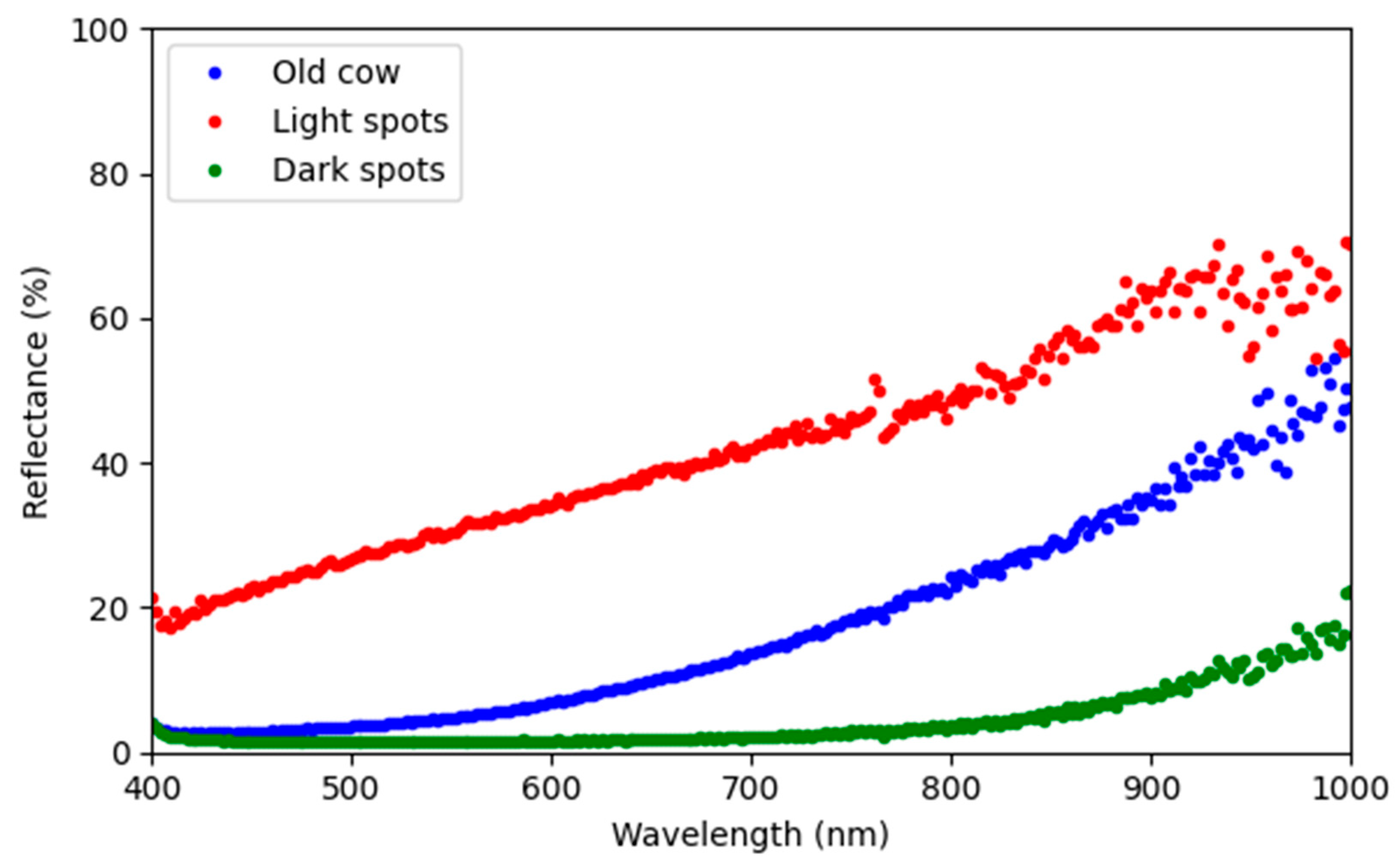
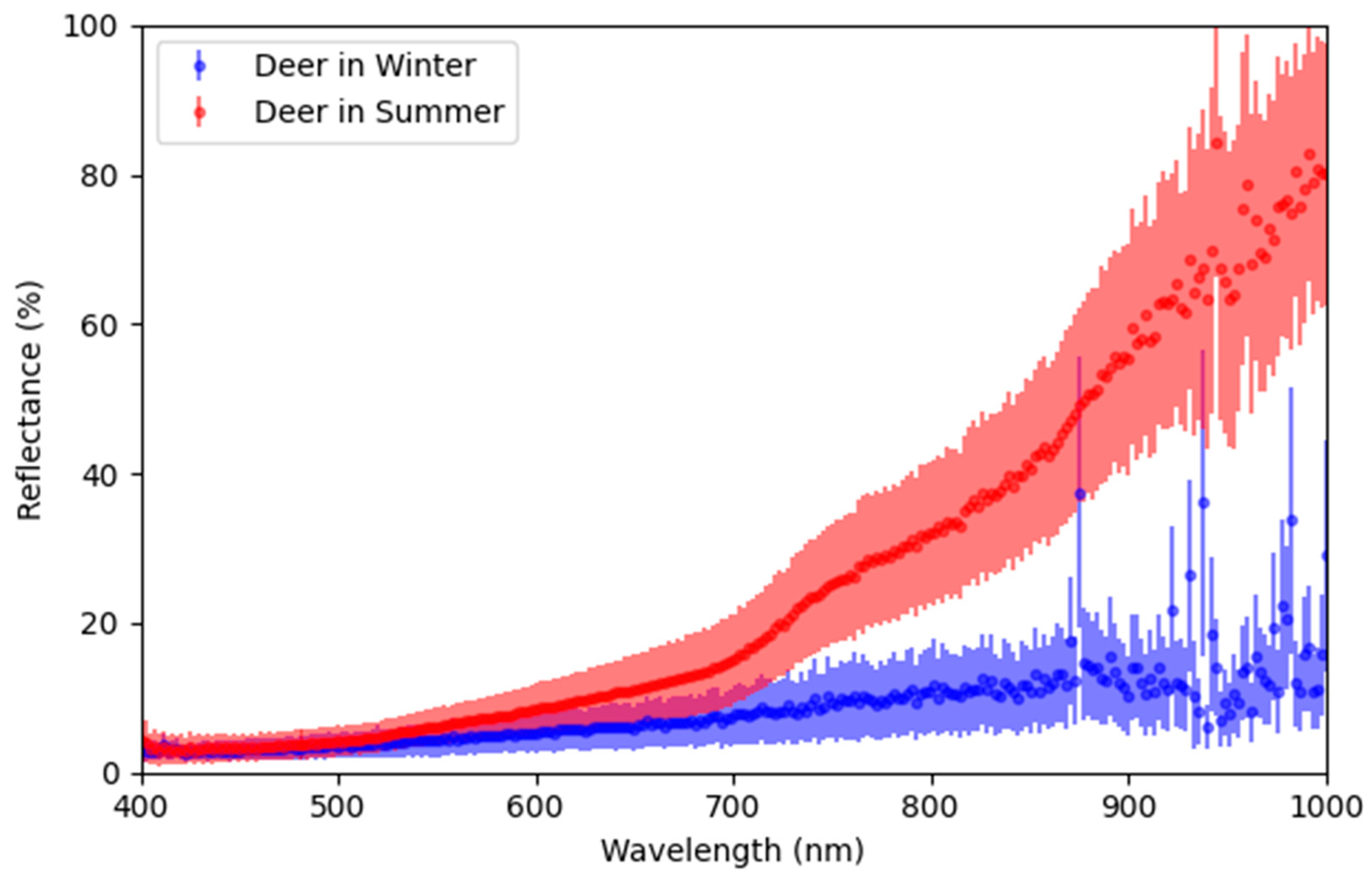
• Creation of a spectral library of four mammal species: cow (Bos taurus), horse (Equus caballus), deer (Odocoileus virginianus), and goat (Capra hircus).
• First study to look at the use of HSI collected by a small UAS to classify terrestrial mammalian species.
• Study the efficacy of neural network and deep machine learning models to classify HSI pixels without using any spatial information.
• Simulate 5-band multispectral data from HSI and test classification efficacy.
• An assessment of the technical feasibility of using spectral features for wildlife detection for invasive species and pest management.

2. Materials and Methods

2.1. Materials

A Headwall Photonics Nano-Hyperspec (Hyperspec VNIR model, Headwall Photonics, Fitchburg, MA, USA) was mounted in a nadir-facing Gremsy S1V2 gimbal attached to a DJI Matrice 600 (SZ DJI Technology Co., Ltd., Shenzhen, China,) uncrewed aerial vehicle. The Nano-Hyperspec is a push broom sensor with a fixed exposure and 640 spatial elements. It has 270 contiguous bands covering the VNIR spectrum (400 nm–1000 nm). With the weight of the Nano-Hyperspec and its independent power source, the UAS had a maximum flight time of roughly 20 min. Figure 1 highlights the locations of data collections. All data were collected in the Starkville Mississippi area with most of the horse and cattle specimens having been collected at the H.H. Leveck Animal Research Center at Mississippi State University. The whitetail deer samples were collected at the Mississippi State University Deer Laboratory. The goat samples were collected at Magowah Ranch located in Artesia, Mississippi. A total of 14 flights were flown and a total of 123 animals were imaged. Most of the imagery was collected during this September to December 2022 timeframe.

Imagery data were collected within two hours of solar noon. Figure 2 shows the UAS platform and camera attached to capture all data used in this study. Push broom sensors with fixed exposures require a larger amount of sensor setup compared to conventional planar array sensors. The flight plan speed and direction must be set up to prioritize data collection quality. Prior to every flight, the exposure and period were set based on the ambient lighting conditions and a collection speed of 5 m/s to ensure square pixels. This 5 m/s upper limit allows for a stable platform and a decent amount of real coverage within a fixed flight time. All data collections were flown at an altitude of 30 m, which resulted in a ground sampling distance of 5 cm. Immediately prior to takeoff, a dark current measurement was recorded for later radiance calculations. Best practices were found to use a geofence over areas of interest, which allowed the sensor to only record data in those areas. All turns over an area were conducted outside of this geofence, and the UAS was in straight and level flight with the sensor oriented so that the scanner was perpendicular to the direction of travel entering the area of interest. A Spectralon (Labsphere, Inc., North Sutton, NH, USA) (99%) white reference panel and an 11% reflectance tarp were in scene during collections for reflectance calculations during post flight processing.

After the data were collected, they were transferred off the sensor to create useable reflectance products. First, the radiance was calculated from the digital number raw data using the dark reference captured prior to flight. Next, the reflectance imagery was calculated based on the calibrated reflectance panel in the imagery. Individual data cubes were orthorectified and conflated to a digital elevation model. Finally, the geolocated single cubes were joined together to create flightlines for spectral signature extraction. Figure 3 shows a collage of images taken from the hyperspectral data. To create these RGB pseudo color images, one band in each respective spectra is taken out of the data cube and stacked together. Figure 3 shows the low spatial resolution of the data collected (5 cm).

2.2. Methods

Reflectance signatures from pixels containing animals were manually extracted by drawing a polygon on the well-illuminated portion of the animal. Care was taken to ensure samples were not extracted close to the edge of the animal to prevent the use of mixed pixels. Similarly, shadowed parts of the animal were not extracted due to lack of information. The shadowed portion reflectance signature was devoid of the defining species characteristics contained in the well-lit portion of the animal. Not every animal imaged was in a lighting condition that facilitated pure pixel extraction due to shadows, animal body orientation, or sun angle.

Table 1. Number of Animals, Pure Samples, Mean and Standard Deviation per Animal per Class.

	Deer	Horse	Cow	Goat	Background
Number of Animals Collected	15	38	30	33	N/A
Pure Pixels Sample Size	219	2351	703	2811	2500
Mean Pure Pixel Samples per Animal	33	168	117	77	N/A
Standard Deviation of Pure Pixel Samples per Animal	29	54	29	37	N/A

shows the number of animals collected and the number of pure pixels extracted from the imagery, as well as the mean and standard deviation of the number of pure pixels per animal.

Reflectance signatures were then stored in a labeled MX270 matrix, where M is the number of pixels residing on the animal and each value of M’s 270 length vector is the value from its corresponding band. Each of these vectors was considered a sample for classification. Similarly, random pixels of the background were extracted from non-shadowed areas. The background class sample size was orders of magnitude larger than the number of samples in the largest animal class. It was subsequently randomly decimated to be of a similar size for model training and testing.

The data were split into training and testing based on the class with the smallest number of samples, which in this case was the deer class. Half of the deer samples were randomly selected for training and the same number of samples from the other classes were selected for training. The remaining samples were used for testing the models.

Table 2. Number of Samples used for Training and Testing the Classification Models.

	Deer	Horse	Cow	Goat	Background
Number of Training Samples	109	109	109	109	109
Number of Testing Samples	110	2242	594	2702	2391

shows the number of samples used for training and testing.

Figure 4 shows the mean spectral signature with the first standard deviation for all species collected. The mean is represented by the dense dots and the standard deviation is shown as the opaque shading. The measured spectra exhibit significant inter and intraspecies variation. The spectral reflectance signature typically depends on variations in the concentrations of chemical constituents or physical properties of the animal’s skin [34,35,39]. Successful classification of the hyperspectral signature depends on the efficacy of various models to extract the desired information from the spectra while ignoring variabilities.

The total number of spectral bands in hyperspectral data is called dimensionality [40]. Each band represents a dimension where the spectra itself is a point in the hyperdimensional space. While high dimensionality of the hyperspectral data offers rich information about the target, it also presents a challenge for machine learning models. This challenge is severe in statistical machine learning and neural networks. In the case of statistical classifiers, the number of labeled samples required to train a machine learning model increases exponentially with the dimension of the data. In neural network-based models, the number of learnable parameters and thus the complexity of the model increases exponentially with the dimension of the data. In the literature, this is referred to as the Hughes phenomenon. Typically, a dimensionality reduction or band selection technique is employed to reduce the dimensions while preserving most of the information distributed throughout the spectra. In this study, to test the maximum likelihood and feed forward neural network, we used a principal component analysis (PCA) and linear discriminant analysis (LDA). In the case of convolutional neural networks (CNN), the filters used to extract information inherently reduce the dimension of the data, thus making the feed forward neural network less complex. Information contained in the hyperspectral data can be used as features to train supervised machine learning models. In this work, we studied the efficacies of maximum likelihood (parametric models), feed forward neural networks, and deep learning neural networks (non-parametric models).

2.2.1. Dimensionality Reduction

Each band in the hyperspectral signature is tightly correlated with each of its neighbors, meaning there is a lot of redundancy in the data. This redundancy can be exploited by discarding some of the data without losing too much information, which is called dimensionality reduction. The four methods of dimensionality reduction investigated were PCA, LDA, forward selection, and backward rejection. PCA projects the data into a new feature space that maximizes the variance of the dataset [41,42]. It allows for the data to be described in far fewer features or principal components based on significant eigenvalues while preserving most of the information [43]. Equation (1) shows the linear transformation of PCA.

$$\overrightarrow{y}=W^T\overrightarrow{x},$$

(1)

LDA also projects the data into a new feature space, but it differs from PCA in that instead of maximizing the variance it attempts to choose a feature space that minimizes the class spread while maximizing the distance between classes [41,42]. This method takes a priori class information into account to allow for discriminating between classes [42]. LDA is a linear transformation similar to PCA, but the transformation matrix is found by solving Equation (2), where S_w and S_b are the within and between class scatter matrices respectively [43].

$${S_w}^{-1}{S}_{b}W=\lambda W,$$

(2)

Forward selection and backwards rejection are both feature selection techniques that keep the data in the original domain. Both techniques iteratively test and train a supervised classification model and either add or subtract features based on the outcome of the model testing. Forward selection starts with no data, adds a band, and then, if that addition increases the classification accuracy, it keeps that band and repeats [44]. If the addition of a band does not increase the classification accuracy, it does not keep that band and moves on to the next. Backwards rejection works similarly to forward selection, but it starts with all of the bands and removes the least impactful band [44]. This iteratively happens until the accuracy no longer increases. Both methods were investigated to see if they would allow a straightforward approach to accurately classifying pixels.

2.2.2. Maximum Likelihood Classification

Parametric models such as the maximum likelihood classifier (MLC) extract class conditional probabilities, mean, and covariance as parameters to learn hyperspectral data [17]. These parameters are then used to construct classification decision boundaries. The MLC is computationally the least expensive but requires a large amount of training samples due to the Hughes phenomenon. This can be partially alleviated by using dimensionality reduction techniques such as principal component analysis (PCA) and linear discriminant analysis (LDA). Although very effective in classifying hyperspectral data, previous studies indicated the limitations of the combinations of PCA, LDA, and MLC [19].

2.2.3. Artificial Neural Networks and 1D Convolutional Networks

Non-parametric models such as feed forward neural networks and support vector machines can learn complex relationships in data better than parametric models such as MLC and Bayesian [23,28]. The neural network-based models are computationally more expensive than parametric models but have the capability to learn subtle differences between classes.

Table 3. Layer Topology of the ANN Used for Classification.

Layer	Layer Name	Output Size	Layer Info	Processing
1	Input	1 × 270 *	-	-
2	Dense	1 × 20	-	ReLU
3	Dense	1 × 8	-	ReLU
4	Dense	1 × 8	-	ReLu
5	Dense	1 × 4 **	-	SoftMax

* Depending on the input of the data. Dimensionality reduction methods lead to smaller output sizes. ** Depending on the number of classes present.

shows the topology of the artificial neural network (ANN). It contains one input layer, three hidden layers, and one output layer. The activation function of the three hidden layers was a rectified linear unit (ReLU), which keeps the value being tested if it is greater than zero. The output layer activation function is a SoftMax [30].

Although MLC and ANN models have been used for the past three decades, they have been shown to produce excellent classification on data that are easily separable. Non-parametric models such as CNN can extract deeper features in the data through a series of filters and thus have the potential to produce excellent classification of data with subtly different classes. For a new exploratory study, we believe testing the efficacy of the above approaches can provide better insight.

The topology of the 1-D CNN used is outlined in

Table 4. Layer Topology of the CNN Used for Classification.

1D Convolutional Network
Layer Name	Output Size	Layer Info	Processing
Input	1 × 270 *	-	-
Conv1D	268 × 32	kernel size = 3	ReLU
MaxPooling1D	89 × 32	pool_size = 3	-
Flatten	1 × 2848	-
Dense	1 × 128	-	ReLu
Dense	1 × 4 **	-	SoftMax

* Depending on the input of the data. Dimensionality reduction methods lead to smaller output sizes. ** Depending on the number of classes present.

. The network contains an input layer, a convolutional layer with a kernel size of 3, that outputs 32 feature maps; a MaxPooling layer that reduces the feature maps by a factor of 3; a flattening layer; one hidden layer; and an output layer. ReLU and SoftMax are used as activation functions.

2.2.4. Simulated Multispectral Classification

HSI measures a continuation of small discrete regions of the light spectrum, resulting in capturing subtle differences in the reflectance of the target. However, for certain applications, sensing in broad regions is sufficient to capture the information required to distinguish classes. Broadband sensors, such as multispectral, measure reflectance over wider ranges of the light spectrum by computing the average reflectance to produce one band. One advantage of capturing broad, widely spaced bands is that the sensor development allows for larger arrays. Most hyperspectral sensors are push broom scanners, but multispectral sensors are typically planar array sensors, which can drastically increase the amount of data captured in the same period.

While no multispectral data were captured, they were simulated by binning the hyperspectral data. The binned bands are an unweighted average of the hyperspectral bands at similar wavelengths, which makes them slightly different than how modern multispectral sensors are manufactured, but it is a close approximation. The multispectral sensor modeled was the Micasense Rededge MX (MicaSense Inc., Seattle, WA, USA) with the following band structure: blue (center wavelength 475 nm, FWHM bandwidth 20 nm), green (560 nm, 20 nm), red (668 nm, 10 nm), red edge (717 nm, 10 nm), and near infrared (840 nm, 40 nm).

The computer used for running the neural network configurations contained an Intel Xeon E5-1630 V3 CPU @ 3.70 GHz with 32 GB of RAM, and an NVIDIA Quadro K2200 GPU. The script for extracting the spectral signatures and MLC were written on MATLAB. For ANN and 1-D CNN, Python (3.11) programming language was used with the following packages: pandas (1.5.3), numpy (1.24.2), sklearn (0.0.post1), tensorflow (2.12.0), matplotlib (3.7.1), and spectral (0.23.1). For the feed-forward neural network models, a categorical cross entropy loss function was used with an Adam optimizer.

2.2.5. Model Evaluation

Each model was evaluated as the predicted class versus the true class via a confusion matrix [45]. The overall accuracy, precision, recall, F1 score, and Cohen’s kappa of each model topology was computed. Overall accuracy is the ratio of the number of correctly identified samples to the total number of samples. While accuracy is a useful metric when analyzing a classifier, it does not tell the whole picture when classes are not well balanced. Since the classes in this study are poorly balanced, precision and recall are more useful metrics to analyze the models [45]. Precision is the ratio between what the classifier correctly identified as belonging to a class divided by the total number of samples it claims belong in that class [45]. Recall is the ratio of correctly identified samples divided by correctly identified samples and samples it incorrectly identified as belonging in that class [45]. Precision and recall are defined in Equations (3) and (4), respectively:

$$\mathrm{Precision}=\frac{\mathrm{N}\mathrm{u}\mathrm{m}\mathrm{b}\mathrm{e}\mathrm{r} \mathrm{o}\mathrm{f} \mathrm{T}\mathrm{r}\mathrm{u}\mathrm{e} \mathrm{P}\mathrm{o}\mathrm{s}\mathrm{i}\mathrm{t}\mathrm{i}\mathrm{v}\mathrm{e}\mathrm{s}}{\mathrm{N}\mathrm{u}\mathrm{m}\mathrm{b}\mathrm{e}\mathrm{r} \mathrm{o}\mathrm{f} \mathrm{T}\mathrm{r}\mathrm{u}\mathrm{e} \mathrm{P}\mathrm{o}\mathrm{s}\mathrm{i}\mathrm{t}\mathrm{i}\mathrm{v}\mathrm{e}\mathrm{s}+\mathrm{N}\mathrm{u}\mathrm{m}\mathrm{b}\mathrm{e}\mathrm{r} \mathrm{o}\mathrm{f} \mathrm{F}\mathrm{a}\mathrm{l}\mathrm{s}\mathrm{e} \mathrm{P}\mathrm{o}\mathrm{s}\mathrm{i}\mathrm{t}\mathrm{i}\mathrm{v}\mathrm{e}\mathrm{s}},$$

(3)

$$\mathrm{Recall}=\frac{\mathrm{N}\mathrm{u}\mathrm{m}\mathrm{b}\mathrm{e}\mathrm{r} \mathrm{o}\mathrm{f} \mathrm{T}\mathrm{r}\mathrm{u}\mathrm{e} \mathrm{P}\mathrm{o}\mathrm{s}\mathrm{i}\mathrm{t}\mathrm{i}\mathrm{v}\mathrm{e}\mathrm{s}}{\mathrm{N}\mathrm{u}\mathrm{m}\mathrm{b}\mathrm{e}\mathrm{r} \mathrm{o}\mathrm{f} \mathrm{T}\mathrm{r}\mathrm{u}\mathrm{e} \mathrm{P}\mathrm{o}\mathrm{s}\mathrm{i}\mathrm{t}\mathrm{i}\mathrm{v}\mathrm{e}\mathrm{s}+\mathrm{N}\mathrm{u}\mathrm{m}\mathrm{b}\mathrm{e}\mathrm{r} \mathrm{o}\mathrm{f} \mathrm{F}\mathrm{a}\mathrm{l}\mathrm{s}\mathrm{e} \mathrm{N}\mathrm{e}\mathrm{g}\mathrm{a}\mathrm{t}\mathrm{i}\mathrm{v}\mathrm{e}\mathrm{s}},$$

(4)

F1 score is the harmonic mean of the precision and recall [45]. It is a preferable metric when classes are imbalanced [45]. This metric spans from zero to one, with one being a perfect classifier [45]. Equation (5) describes the calculation of the F1 score:

$$\mathrm{F}1\text{-Score}=\frac{\mathrm{P}\mathrm{r}\mathrm{e}\mathrm{c}\mathrm{i}\mathrm{s}\mathrm{i}\mathrm{o}\mathrm{n}\ast \mathrm{R}\mathrm{e}\mathrm{c}\mathrm{a}\mathrm{l}\mathrm{l}}{\mathrm{P}\mathrm{r}\mathrm{e}\mathrm{c}\mathrm{i}\mathrm{s}\mathrm{i}\mathrm{o}\mathrm{n}+\mathrm{R}\mathrm{e}\mathrm{c}\mathrm{a}\mathrm{l}\mathrm{l}},$$

(5)

Cohen’s kappa is a metric that looks at interrater reliability [46]. For the purposes of this study, it looks at the degree of agreement between each samples’ assigned class and labeled class while accounting for the possibility that the classifier correctly assigned a class by chance [46]. It spans from −1 to 1, with any value greater than 0 meaning that the agreement was based on more than pure chance [47]. Ranges from 0.6 to 0.8 are considered as having substantial agreement and ranges 0.8 to 1 as almost perfect agreement [47].

3. Results

3.1. Dimensionality Reduction

When using PCA for dimensionality reduction, the top twenty principal components were kept for classification. We repeated the training with different numbers of principal components from 5 to 30 to determine the ideal number. The accuracy metrics of the model showed improvement between 5 to 20 and after that, no significant improvement was observed. LDA results in C-1 dimensions where C is the number of classes. For this study, that resulted in four dimensions. The forward selection method of dimensionality reduction resulted in keeping bands at 429 nm, 547 nm, 650 nm, 732 nm, 828 nm, and 962 nm. These wavelengths correspond to a single band in the blue, green, red, and red edge, and two bands spanning the NIR spectrum. The backwards rejection method yielded slightly different results. It highlighted keeping bands at 400 nm, 411 nm, 552 nm, 625 nm, 793 nm, 797 nm, 871 nm, and 973 nm, which correspond to two bands in the blue spectrum, one in the green, one in the red, and four throughout the NIR spectrum.

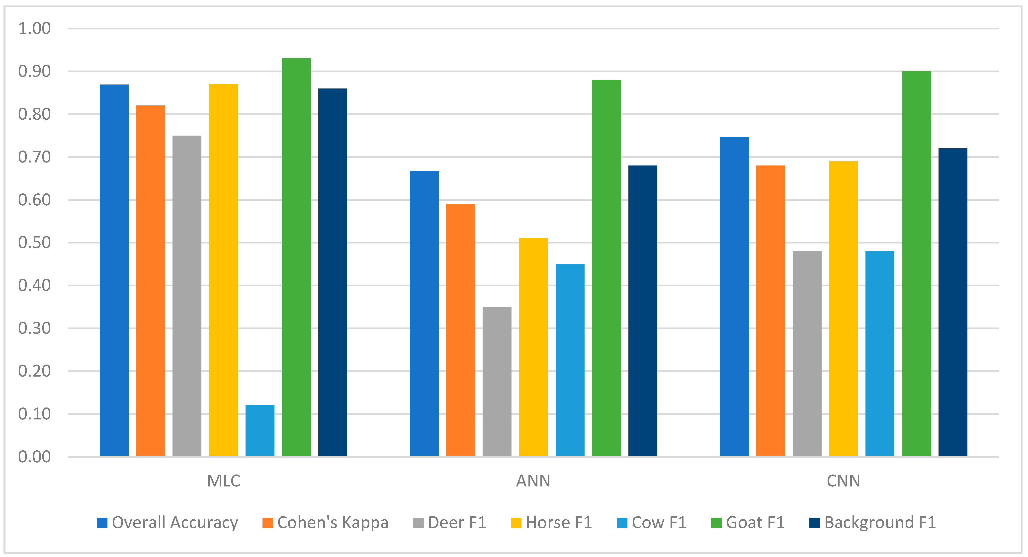
3.2. Model Performance

The MLC produced a best overall accuracy of more than 98% with the LDA dimensionality reduction technique; however, the class F1 scores and Cohen’s kappa were not as high as with PCA. MLC-PCA resulted in the lowest overall accuracy but had the highest kappa and class F1 scores. The forward selection and backwards rejection techniques showed middling results, with most classes having greater than 0.75 F1 scores. Both forward selection and backwards rejection resulted in lower F1 scores than PCA. Figure 5 details the overall accuracy, Cohen’s kappa, and each class F1 score for each dimensionality reduction technique tested with the MLC classifier.

The artificial neural network (ANN) was tested with all 270 bands in the hyperspectral data along with the four feature reduction methods used with MLC. The ANN produced a best overall accuracy of more than 98% and the highest consistent kappa and class F1 scores when reducing dimensionality via LDA. Full dimensionality and reduced dimensionality in transformed spaces outperformed forward selection and backward rejection by a wide margin across all metrics. The class F1 scores, Cohen’s kappa, and overall accuracy for each case considered are shown in Figure 6. These experiments were repeated for different numbers of epochs, and we observed no significant benefit in training these models beyond 50 epochs.

Results from the ANN experiments did not drastically improve the performance achieved through a statistical model such as MLC. These experiments were repeated with a 1-D convolutional neural network (CNN), where a series of filters were learned as part of the supervised training process. The CNN model was tested with all 270 bands in the hyperspectral data along with the same four feature reduction methods used with MLC and ANN. The 1-D CNN produced the best overall accuracy and consistently higher F1 scores with LDA dimensionality reduction. When classifying with feature reduction techniques, both PCA and LDA performed better than full dimensionality. The overall accuracy and class precision and recall of the 1D CNN experiments did not show improvements over the ANN and had no significant improvements over MLC. The class F1 scores, Cohen’s kappa, and overall accuracy for each case considered are shown in Figure 7 for the CNN classifier. These experiments were repeated for different numbers of epochs, and we observed no significant benefit in training these models beyond 50 epochs.

The simulated five-band multispectral data classification performed reasonably well. The same models tested on the hyperspectral signatures were tested on the binned five-band data. The MLC was able to classify most of the classes better than the ANN and CNN when using the F1 scores as a metric. However, the cow class F1 score was drastically lower than the other classes, which reflects a poor ability to correctly classify cows. The ANN classifier had much lower class F1 scores than the MLC and slightly lower F1 scores than the CNN. The CNN classifier performed slightly better than the ANN and slightly poorer than the MLC. Figure 8 details the overall accuracy, Cohen’s kappa, and class F1 scores for the models trained and tested on simulated five-band multispectral data.

4. Discussion

Our results show that it is technically feasible to use hyperspectral data without spatial information to distinguish between certain types of mammals and their surroundings using relatively low sample sizes. The results insinuate that a single, clear pixel is enough information to accurately classify the animals investigated. This is important in settings where animals are under canopy cover and might only be partially visible. Our classification efforts show that there seems to be no benefit in using more complicated methods of ANN and CNN when MLC performed as well or better.

However, there are significant challenges that can arise in the classification process. One main challenge is the intraspecies variation of certain mammals, as has been described elsewhere and further expanded by our study [39]. Some of these intraspecies variations occur from pigment variations and some are thought to be attributed to the angle and orientation of the reflected light [34].

In Figure 4 the spectral signatures from the goats had a much larger variation than any of the other species. The goats also had a much higher mean reflectance in the visible spectrum. Both metrics being so elevated is most likely due to the lighter color of the goats we imaged. Most of the cows in the dataset were dark brown or black, and most of the goats were light brown, cream, or white, which reflect significantly more light in the visible spectrum than the dark brown and black of the cows. Figure 9 shows how even a multicolored cow can display different spectral signatures from different regions on the same animal. Different colored animals of the same species need to be concurrently collected and the data investigated for bands invariant to color in line with the findings of Aslett and Garza and Bortolot and Prater [34,39].

Another challenge when classifying via spectral signature is the presence of shadows and occlusions. An animal may be visible beneath a canopy, but the signature from the visible pixels will be highly subdued and repressed if it is in shadow. The spectral signature still has the same curve and shape as a well-lit sample, but the reflectance values are so low that they might not be useable to positively identify the animal. However, if a target is partially occluded but the visible portion is well lit then there is a good chance of accurate classification.

An additional challenge encountered was temporal variations in spectral signatures due to seasonal coat changes. We collected additional samples of white-tailed deer six months after the original collection, in May 2023, and noticed that the spectral signature was vastly different than the samples collected in December. Figure 10 shows the difference in the reflectance signatures from the two data collections. The summer data starts to deviate around the 600 nm region and continues to increase the separation from the original data well into the near infrared region. The visible portion of this deviation is seen as a reddish tint in the summer months, but it was unexpected to have such a drastic difference in the NIR spectrum. Since we only acquired the deer imagery at two dates, we are not sure about the variations in reflectance that might occur throughout the year. Future research should look at collecting HSI in controlled environments throughout the year and study the temporal variabilities in the spectra. This variation throughout the year could make it difficult for a model to accurately classify a deer sample.

The findings from the different classification methods show that the MLC can accurately classify the data and there does not seem to be much of a benefit in using more computationally expensive methods such as ANN and CNN. The dimensionality reduction techniques insinuate that LDA is the best option for the data under investigation, but that all methods analyzed performed well. One caveat to the better performance of the LDA in the forward selection and backward rejection is that since both iterative methods remain in the original space, they can be represented via physical sensors. This means a sensor could be developed with the same or similar bands at a reduced cost when compared to the full hyperspectral sensor and could potentially capture a substantially larger amount of areal data in a similar time period. This proposed sensor would take care of the dimensionality reduction by only capturing pertinent bands for classification.

Our experiments with the simulated five-band data showed a decent ability to differentiate classes. This is promising because there are numerous commercially available sensors available with different band spacing and bandwidth. A similar study has shown the feasibility of using multispectral imaging to detect polar bears [37]. Chabot et al.’s results and our simulated multispectral classification show the potential to use multispectral data to be able to classify invasive mammal species [37]. These sensors are also two-dimensional arrays, which would lead to far more data being collected in the same time span as a push broom sensor. These findings resonate with Colefax et al., who found specific wavelengths to identify marine animals and that high spatial resolution imaging would benefit the classification and identification process [48]. With a two-dimensional sensor, the spatial relationship and other morphological features of the animals can be better extracted to increase the amount of features available for recognition. Further investigation should consider the possibility of classification via commercially available broadband multispectral sensors.

While highly accurate classifications of natural and artificial materials based on spectral information could potentially overcome some of the barriers associated with traditional sensors, the significant costs and expertise to use these sensors and process and analyze the hyperspectral datasets are not cost-effective. One hurdle with using a push broom HSI versus traditional RGB imagery is the additional effort it takes to create quality data products. The sensor setup for collection is significantly more involved due to the sensor topology and the post flight processing is more time consuming and detail driven. Additionally, due to a fixed exposure, variable lighting conditions will significantly impact reflectance products. However, a RGB sensor would not allow for single or pixel classification of target species. This study highlights the need to perform an exhaustive investigation, comparing various methods and sensor types for monitoring invasive species, including conventional RGB, thermal, multispectral, and hyperspectral sensors.

Future studies should investigate (1) creating a large library of spectral signatures of animals captured throughout the year and of all available colors, (2) applying a similar methodology from this paper using a multispectral sensor at or around the wavelengths identified via forward selection and/or backwards rejection, and (3) detailed cost-benefit analyses of commercial UAS remote sensing sensors.

Our results show promise that animal species can be detected and classified using only spectral characteristics from relatively low sample sizes and we identified additional spectra not previously used for animal detection that can improve species-specific classification accuracy, something that could greatly improve the efficiency of invasive species management on islands. Further investigation is needed to evaluate how to incorporate these additional spectra into practical, cost-effective sensors and analytics workflows that could measurably improve operational decision making. Using only spectra to uniquely classify materials of interest raises the possibility of simplified on-board analytics, something currently lacking in the majority of commercially available visible and thermal sensor and analytics offerings. This study provides a foundation for continued research into this area and encourages a broader exploration of how spectra may improve invasive species detection and management efforts.

References

1. Tershy, B.R.; Shen, K.-W.; Newton, K.M.; Holmes, N.D.; Croll, D.A. The Importance of Islands for the Protection of Biological and Linguistic Diversity. BioScience 2015, 65, 592–597. [Google Scholar] [CrossRef]
2. Spatz, D.R.; Holmes, N.D.; Will, D.J.; Hein, S.; Carter, Z.T.; Fewster, R.M.; Keitt, B.; Genovesi, P.; Samaniego, A.; Croll, D.A.; et al. The global contribution of invasive vertebrate eradication as a key island restoration tool. Sci. Rep. 2022, 12, 13391. [Google Scholar] [CrossRef] [PubMed]
3. Jones, H.P.; Holmes, N.D.; Butchart, S.H.M.; Tershy, B.R.; Kappes, P.J.; Corkery, I.; Aguirre-Muñoz, A.; Armstrong, D.P.; Bonnaud, E.; Burbidge, A.A.; et al. Invasive mammal eradication on islands results in substantial conservation gains. Proc. Natl. Acad. Sci. USA 2016, 113, 4033–4038. [Google Scholar] [CrossRef] [PubMed]
4. Kappes, P.J.; Benkwitt, C.E.; Spatz, D.R.; Wolf, C.A.; Will, D.J.; Holmes, N.D. Do Invasive Mammal Eradications from Islands Support Climate Change Adaptation and Mitigation? Climate 2021, 9, 172. [Google Scholar] [CrossRef]
5. de Wit, L.A.; Zilliacus, K.M.; Quadri, P.; Will, D.; Grima, N.; Spatz, D.; Holmes, N.; Tershy, B.; Howald, G.R.; A Croll, D. Invasive vertebrate eradications on islands as a tool for implementing global Sustainable Development Goals. Environ. Conserv. 2020, 47, 139–148. [Google Scholar] [CrossRef]
6. Sandin, S.A.; Becker, P.A.; Becker, C.; Brown, K.; Erazo, N.G.; Figuerola, C.; Fisher, R.N.; Friedlander, A.M.; Fukami, T.; Graham, N.A.J.; et al. Harnessing island–ocean connections to maximize marine benefits of island conservation. Proc. Natl. Acad. Sci. USA 2022, 119, e2122354119. [Google Scholar] [CrossRef]
7. Rodrigues, A.S.L.; Brooks, T.M.; Butchart, S.H.M.; Chanson, J.; Cox, N.; Hoffmann, M.; Stuart, S.N. Spatially Explicit Trends in the Global Conservation Status of Vertebrates. PLoS ONE 2014, 9, e113934. [Google Scholar] [CrossRef] [PubMed]
8. Fricke, R.M.; Olden, J.D. Technological innovations enhance invasive species management in the anthropocene. BioScience 2023, 73, 261–279. [Google Scholar] [CrossRef]
9. Campbell, K.J.; Beek, J.; Eason, C.T.; Glen, A.S.; Godwin, J.; Gould, F.; Holmes, N.D.; Howald, G.R.; Madden, F.M.; Ponder, J.B.; et al. The next generation of rodent eradications: Innovative technologies and tools to improve species specificity and increase their feasibility on islands. Biol. Conserv. 2015, 185, 47–58. [Google Scholar] [CrossRef]
10. Martinez, B.; Reaser, J.K.; Dehgan, A.; Zamft, B.; Baisch, D.; McCormick, C.; Giordano, A.J.; Aicher, R.; Selbe, S. Technology innovation: Advancing capacities for the early detection of and rapid response to invasive species. Biol. Invasions 2019, 22, 75–100. [Google Scholar] [CrossRef]
11. Campbell, K.J.; Harper, G.; Algar, D.; Hanson, C.C.; Keitt, B.S.; Robinson, S. Review of feral cat eradications on islands. Isl. Invasives Erad. Manag. 2011, 37, 46. [Google Scholar]
12. Carrion, V.; Donlan, C.J.; Campbell, K.J.; Lavoie, C.; Cruz, F. Archipelago-Wide Island Restoration in the Galápagos Islands: Reducing Costs of Invasive Mammal Eradication Programs and Reinvasion Risk. PLoS ONE 2011, 6, e18835. [Google Scholar] [CrossRef] [PubMed]
13. Anderson, D.P.; Gormley, A.M.; Ramsey, D.S.L.; Nugent, G.; Martin, P.A.J.; Bosson, M.; Livingstone, P.; Byrom, A.E. Bio-economic optimisation of surveillance to confirm broadscale eradications of invasive pests and diseases. Biol. Invasions 2017, 19, 2869–2884. [Google Scholar] [CrossRef]
14. Davis, R.A.; Seddon, P.J.; Craig, M.D.; Russell, J.C. A review of methods for detecting rats at low densities, with implications for surveillance. Biol. Invasions 2023, 25, 3773–3791. [Google Scholar] [CrossRef]
15. Krishnan, B.S.; Jones, L.R.; Elmore, J.A.; Samiappan, S.; Evans, K.O.; Pfeiffer, M.B.; Blackwell, B.F.; Iglay, R.B. Fusion of visible and thermal images improves automated detection and classification of animals for drone surveys. Sci. Rep. 2023, 13, 10385. [Google Scholar] [CrossRef]
16. Schneider, S.; Greenberg, S.; Taylor, G.W.; Kremer, S.C. Three critical factors affecting automated image species recognition performance for camera traps. Ecol. Evol. 2020, 10, 3503–3517. [Google Scholar] [CrossRef]
17. Vélez, J.; McShea, W.; Shamon, H.; Castiblanco-Camacho, P.J.; Tabak, M.A.; Chalmers, C.; Fergus, P.; Fieberg, J. An evaluation of platforms for processing camera-trap data using artificial intelligence. Methods Ecol. Evol. 2022, 14, 459–477. [Google Scholar] [CrossRef]
18. Morellet, N.; Gaillard, J.; Hewison, A.J.M.; Ballon, P.; Boscardin, Y.; Duncan, P.; Klein, F.; Maillard, D. Indicators of ecological change: New tools for managing populations of large herbivores: Ecological indicators for large herbivore management. J. Appl. Ecol. 2007, 44, 634–643. [Google Scholar] [CrossRef]
19. Elmore, J.A.; Schultz, E.A.; Jones, L.R.; Evans, K.O.; Samiappan, S.; Pfeiffer, M.B.; Blackwell, B.F.; Iglay, R.B. Evidence on the efficacy of small unoccupied aircraft systems (UAS) as a survey tool for North American terrestrial, vertebrate animals: A systematic map. Environ. Evid. 2023, 12, 3. [Google Scholar] [CrossRef]
20. Joyce, K.E.; Anderson, K.; Bartolo, R.E. Of Course We Fly Unmanned—We’re Women! Drones 2021, 5, 21. [Google Scholar] [CrossRef]
21. Lenzi, J.; Barnas, A.F.; ElSaid, A.A.; Desell, T.; Rockwell, R.F.; Ellis-Felege, S.N. Artificial intelligence for automated detection of large mammals creates path to upscale drone surveys. Sci. Rep. 2023, 13, 947. [Google Scholar] [CrossRef]
22. Jiménez-Torres, M.; Silva, C.P.; Riquelme, C.; Estay, S.A.; Soto-Gamboa, M. Automatic Recognition of Black-Necked Swan (Cygnus melancoryphus) from Drone Imagery. Drones 2023, 7, 71. [Google Scholar] [CrossRef]
23. Zhou, M.; Elmore, J.A.; Samiappan, S.; Evans, K.O.; Pfeiffer, M.B.; Blackwell, B.F.; Iglay, R.B. Improving Animal Monitoring Using Small Unmanned Aircraft Systems (sUAS) and Deep Learning Networks. Sensors 2021, 21, 5697. [Google Scholar] [CrossRef] [PubMed]
24. Thomas, C.; Ranchin, T.; Wald, L.; Chanussot, J. Synthesis of Multispectral Images to High Spatial Resolution: A Critical Review of Fusion Methods Based on Remote Sensing Physics. IEEE Trans. Geosci. Remote Sens. 2008, 46, 1301–1312. [Google Scholar] [CrossRef]
25. van der Meer, F.D.; van der Werff, H.M.A.; van Ruitenbeek, F.J.A.; Hecker, C.A.; Bakker, W.H.; Noomen, M.F.; van der Meijde, M.; Carranza, E.J.M.; de Smeth, J.B.; Woldai, T. Multi- and hyperspectral geologic remote sensing: A review. Int. J. Appl. Earth Observ. Geoinf. 2012, 14, 112–128. [Google Scholar] [CrossRef]
26. Ghiyamat, A.; Shafri, H.Z.M. A review on hyperspectral remote sensing for homogeneous and heterogeneous forest biodiversity assessment. Int. J. Remote. Sens. 2010, 31, 1837–1856. [Google Scholar] [CrossRef]
27. Matese, A.; Czarnecki, J.; Samiappan, S.; Moorhead, J. Are unmanned aerial vehicle based hyperspectral imaging and machine learning advancing crop science? Trends Plant Sci. 2023. [Google Scholar] [CrossRef]
28. Murphy, P.K.; Kolodner, M.A. Implementation of a Multiscale Bayesian Classification Approach for Hyperspectral Terrain Categorization. Proc. SPIE 2022, 4816, 278–287. [Google Scholar] [CrossRef]
29. Camps-Valls, G.; Gómez-Chova, L.; Calpe-Maravilla, J.; Soria-Olivas, E.; Martín-Guerrero, J.D.; Moreno, J. Support Vector Machines for Crop Classification Using Hyperspectral Data. In Proceedings of the 1st Pattern Recognition and Image Analysis, Puerto de Andratx, Mallorca, Spain, 4–6 June 2003; pp. 134–141. [Google Scholar] [CrossRef]
30. Chen, Y.; Lin, Z.; Zhao, X.; Wang, G.; Gu, Y. Deep Learning-Based Classification of Hyperspectral Data. IEEE J. Sel. Top. Appl. Earth Obs. Remote Sens. 2014, 7, 2094–2107. [Google Scholar] [CrossRef]
31. Goel, P.; Prasher, S.; Patel, R.; Landry, J.; Bonnell, R.; Viau, A. Classification of hyperspectral data by decision trees and artificial neural networks to identify weed stress and nitrogen status of corn. Comput. Electron. Agric. 2003, 39, 67–93. [Google Scholar] [CrossRef]
32. Kolmann, M.A.; Kalacska, M.; Lucanus, O.; Sousa, L.; Wainwright, D.; Arroyo-Mora, J.P.; Andrade, M.C. Hyperspectral data as a biodiversity screening tool can differentiate among diverse Neotropical fishes. Sci. Rep. 2021, 11, 16157. [Google Scholar] [CrossRef] [PubMed]
33. Krekeler, M.P.S.; Burke, M.; Allen, S.; Sather, B.; Chappell, C.; McLeod, C.L.; Loertscher, C.; Loertscher, S.; Dawson, C.; Brum, J.; et al. A novel hyperspectral remote sensing tool for detecting and analyzing human materials in the environment: A geoenvironmental approach to aid in emergency response. Environ. Earth Sci. 2023, 82, 109. [Google Scholar] [CrossRef]
34. Bortolot, Z.J.; Prater, P.E. A first assessment of the use of high spatial resolution hyperspectral imagery in discriminating among animal species, and between animals and their surroundings. Biosyst. Eng. 2009, 102, 379–384. [Google Scholar] [CrossRef]
35. Terletzky, P.; Ramsey, R.D.; Neale, C.M.U. Spectral Characteristics of Domestic and Wild Mammals. GIScience Remote Sens. 2012, 49, 597–608. [Google Scholar] [CrossRef]
36. Siers, S.R.; Swayze, G.A.; Mackessey, S.P. Spectral analysis reveals limited potential for enhanced-wavelength detection of invasive snakes. Herpetol. Rev. 2013, 44, 56–58. [Google Scholar]
37. Chabot, D.; Stapleton, S.; Francis, C.M. Measuring the spectral signature of polar bears from a drone to improve their detection from space. Biol. Conserv. 2019, 237, 125–132. [Google Scholar] [CrossRef]
38. Leblanc, G.; Francis, C.M.; Soffer, R.; Kalacska, M.; De Gea, J. Spectral Reflectance of Polar Bear and Other Large Arctic Mammal Pelts; Potential Applications to Remote Sensing Surveys. Remote Sens. 2016, 8, 273. [Google Scholar] [CrossRef]
39. Aslett, Z.; Garza, L. Characterization of Domestic Livestock and Associated Agricultural Facilities using NASA/JPL AVIRIS-NG Imaging Spectroscopy Data. In Proceedings of the 2021 11th Workshop on Hyperspectral Imaging and Signal Processing: Evolution in Remote Sensing (WHISPERS), Amsterdam, The Netherlands, 24–26 March 2021; pp. 1–5. [Google Scholar]
40. Agrawal, N.; Verma, K. Dimensionality Reduction on Hyperspectral Data Set. In Proceedings of the 2020 First International Conference on Power, Control and Computing Technologies (ICPC2T), Raipur, India, 3–5 January 2020; pp. 139–142. [Google Scholar]
41. Lv, W.; Wang, X. Overview of Hyperspectral Image Classification. J. Sens. 2020, 2020, 4817234. [Google Scholar] [CrossRef]
42. Duda, R.O.; Hart, P.E.; Stork, D.G. Pattern Classification, 2nd ed.; Wiley: New York, NY, USA, 2001. [Google Scholar]
43. Prasad, S.; Bruce, L.M. Limitations of principal components analysis for hyperspectral target recognition. IEEE Geosci. Remote Sens. Lett. 2008, 5, 625–629. [Google Scholar] [CrossRef]
44. Pudil, P.; Novovičová, J.; Kittler, J. Floating search methods in feature selection. Pattern Recognit. Lett. 1994, 15, 1119–1125. [Google Scholar] [CrossRef]
45. Tharwat, A. Classification assessment methods. Appl. Comput. Inform. 2018, 17, 168–192. [Google Scholar] [CrossRef]
46. Cohen, J. A Coefficient of Agreement for Nominal Scales. Educ. Psychol. Meas. 1960, 20, 37–46. [Google Scholar] [CrossRef]
47. Landis, J.R.; Koch, G.G. The Measurement of Observer Agreement for Categorical Data. Biometrics 1977, 33, 159–174. [Google Scholar] [CrossRef] [PubMed]
48. Colefax, A.P.; Walsh, A.J.; Purcell, C.R.; Butcher, P. Utility of Spectral Filtering to Improve the Reliability of Marine Fauna Detections from Drone-Based Monitoring. Sensors 2023, 23, 9193. [Google Scholar] [CrossRef]
Figure 1. Locations near Starkville, MS USA where the hyperspectral imagery of four mammalian species were acquired (marked as yellow stars). Deer were collected at the M.S.U. Deer Laboratory. Horses and cows were collected at the H.H. Leveck Research Park. Goats were collected at Magowah Ranch.
Remotesensing 16 00406 g001
Figure 2. DJI Matrice 600 UAS mounted with a Headwall Nano Hyperspectral camera with a Gremsy gimbal.
Remotesensing 16 00406 g002
Figure 3. Visible bands from hyperspectral data of four mammalian species (A) deer, (B) goat, (C) horse and (D) cow.
Remotesensing 16 00406 g003
Figure 4. Averaged hyperspectral reflectance, including standard deviation for four mammalian species and vegetation background considered for this study.
Remotesensing 16 00406 g004
Figure 5. This figure shows the overall accuracy in blue, Cohen’s kappa in orange, deer F1 score in gray, horse F1 score in yellow, cow F1 score in light blue, goat F1 in green, and background F1 in navy for the MLC classification. Each cluster represents the type of dimensionality reduction used.
Remotesensing 16 00406 g005
Figure 6. This figure shows the overall accuracy in blue, Cohen’s kappa in orange, deer F1 score in gray, horse F1 score in yellow, cow F1 score in light blue, goat F1 in green, and background F1 in navy for the ANN classification. Each cluster represents the type of dimensionality reduction used.
Remotesensing 16 00406 g006
Figure 7. This figure shows the overall accuracy in blue, Cohen’s kappa in orange, deer F1 score in gray, horse F1 score in yellow, cow F1 score in light blue, goat F1 in green, and background F1 in navy for the CNN classification. Each cluster represents the type of dimensionality reduction used.
Remotesensing 16 00406 g007
Figure 8. This figure shows the overall accuracy in blue, Cohen’s kappa in orange, deer F1 score in gray, horse F1 score in yellow, cow F1 score in light blue, goat F1 in green, and background F1 in navy for the MLC, ANN, and CNN classifiers on the simulated 5-band data.
Remotesensing 16 00406 g008
Figure 9. Averaged hyperspectral reflectance of a cow (blue) with dark colored spots (red) and light or white colored spots (green).
Remotesensing 16 00406 g009
Figure 10. Averaged hyperspectral reflectance, including standard deviation, for deer samples in the summer (red) and winter (blue).
Remotesensing 16 00406 g010