Abstract
The variation of lake water storage is an important indicator for studying both climate change and ecological environment changes. Previous studies have mainly focused on the lake storage changes in recent decades, and predicting future lake storage changes on the Tibetan Plateau under climate change scenarios remains a crucial gap. We addressed this gap by establishing prediction models for water storage changes in nine lakes using historical water storage and climate data from the past 29 years and predicting the water storage changes for the next 80 years under three scenarios based on Phase 6 of the Coupled Model Intercomparison Project (CMIP6) data. The Quantile-mapping (QM) method was applied to correct the precipitation data of CMIP6 with assimilated data. The results indicated that the prediction model performed well, with high correlation (R2 > 0.7 for the training set) and low mean absolute error (MSE < 0.1 km3). The results suggest that most lakes will experience a slight increase in water storage until 2050, followed by a rapid rise until 2100 under all three SSP (Shared Socioeconomic Pathways) scenarios, including SSP126, SSP245, and SSP585. By the end of the century, the total projected increase in lake water storage is estimated to be 189.676 ± 16.266 km3, 191.762 ± 10.683 km3, and 186.212 ± 6.441 km3 until 2100, respectively.
1. Introduction
The Tibetan Plateau (TP) is the highest and largest plateau in the world, with an average elevation exceeding 4000 m. It is known as the “Roof of the World” and the “Water Tower of Asia”. Under the background of global warming, the global and regional water cycle has undergone significant changes [1,2]. According to the Intergovernmental Panel on Climate Change (IPCC) report [3,4], the global average surface temperature increased by 1.09 ± 0.1 °C between 2011 and 2020, compared to the period between 1850 and 1900. Precipitation has also increased over the past few decades, especially in the central Tibetan Plateau [5]. The changes in the hydrological cycle of the Tibetan Plateau had a profound impact on glacial meltwater, permafrost degradation, and lake expansion. Lake expansion can inundate grasslands and pastures, with serious consequences for local ecosystems, regional water balance, and the economy. Additionally, lakes are important components of wetlands, safeguarding endangered species and playing a vital role in preserving ecosystem diversity.
A vast expanse of glaciers, lakes, and permafrost covers the TP, home to over 1000 lakes encompassing a total area of over 46,500 km2, accounting for about 50% of the total lake area in China. These plateau lakes serve as sensitive indicators of climate change due to their unique geographical location and environment, with most being closed systems and less affected by human activities. Numerous studies have focused on the changing characteristics of these plateau lakes, including area changes [6,7,8], water level dynamics [9,10,11], and water storage variations [12,13,14,15]. Zhang et al. [15], employing multi-temporal Landsat (MSS, TM, ETM+, OLI) satellite imagery, altimetry data, or bathymetry data, found that the total area of lakes on the TP (>1 km2) was 4.0 × 10⁴ ± 766.5 km2 in 1976, expanding around 10,000 km2 by 2018. Utilizing ICESat-2 data, Zhang et al. [16] observed a rising trend among most of these lakes, indicating an average water level change rate of 0.28 ± 0.03 m/y in 62 lakes during the period 2003~2018 on the TP. Based on the Shuttle Radar Topography Mission Digital Elevation Model (SRTM DEM) and Landsat imagery, Yang et al. [17] suggested a significant increase in the water storage of lakes (>50 km2) on the TP from 2.77 km3/y from 1976 to 2013 to 7.67 km3/y from 2000 to 2013. Qiao et al. [13] suggested an expansion of lake water storage changes of 315 lakes (>10 km2) amounting to 140.8 Gt during 1990–2013 on the TP. Furthermore, Yao et al. [18] estimated an increase in lake water storage by 95.42 ± 8.06 km3 during 2002~2015. Through water balance analysis, Zhang et al. [19] concluded that the primary driver of lake expansion (74%) on the TP was the increase in net precipitation, followed by glacier mass loss (13%) and ground ice melting caused by permafrost degradation (12%).
The Coupled Model Intercomparison Project (CMIP) was launched in 1995, providing simulations not only for historical periods but also for future climate change under different carbon emission scenarios. This has generated a large number of fundamental data for global climate change research [20,21]. CMIP has evolved into its sixth stage, with the latest generation of models incorporating more sophisticated parameterization schemes, flux processing methods, and coupler technologies [22]. Zhang et al. [23] indicated that Phase 5 of the Coupled Model Intercomparison Project (CMIP5) had large systematic errors, especially for precipitation. Huang et al. [24] employed four transfer functions of Quantile-mapping (QM) to correct the monthly precipitation of different Representative Concentration Pathways (RCPs) scenarios in the global climate models. In addition, many studies have utilized CMIP model simulations to assess and predict climate change on the TP [25,26,27,28]. Under a 2 °C global warming scenario, Wang et al. [29] suggested that the TP will experience increased precipitation, with a higher increase in the monsoon region (3.9%) compared with the westerly region (0.8%), and the total runoff of major rivers is projected to be 4.1% during the wet season. Amengual et al. [30] predicted that most of the continuous permafrost on the TP will disappear until 2050 under three future scenario models, with an estimated permafrost area loss of 44.4%, 59.5%, and 71.7% by the end of the 21st century, respectively. Based on CMIP5 temperature and precipitation anomalies, Anderson et al. [31] suggested that the glaciers will shrink by 248 ± 66 mm of sea level equivalent (RCP2.6), 313 ± 50 mm of sea level equivalent (RCP4.5), or 424 ± 46 mm of sea level equivalent (RCP8.5) under three future scenarios, respectively.
At present, numerous studies focus on predicting changes in river runoff, permafrost degradation, and glacier extent in the future. However, in the context of climate change, there remains a gap in the research examining how lakes on the TP will evolve. Predicting lake water storage changes can be helpful in managing water resources on the TP. Therefore, the study will address the following aspects: (1) selection of 20 temperature, precipitation, and evaporation models from CMIP6, followed by correcting precipitation data by integrating with the China meteorological forcing dataset (CMFD); (2) construction of a lake water storage change prediction model using the random forest algorithm incorporating historical annual lake water storage change and climate data; (3) analysis of lake water storage changes over the next 80 years using the corrected CMIP6 data and the prediction model under three different scenarios.
2. Study Area and Data
2.1. Study Area
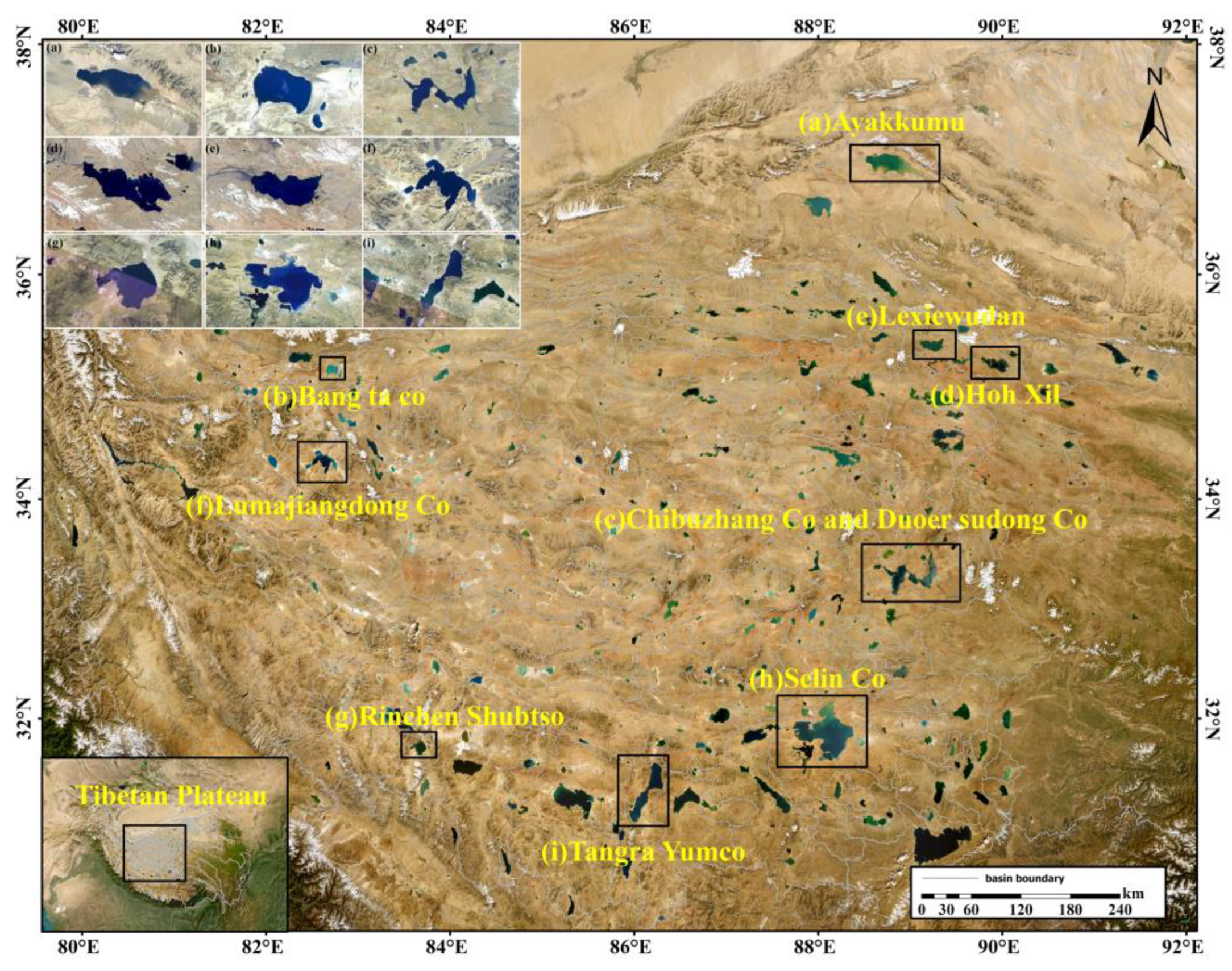
The TP is home to a vast expanse of glaciers, lakes, and permafrost, all situated within a cold and dry climate, characterized by intense solar radiation and high evaporation intensity. Most lakes are closed ecosystems, are less affected by human activity, and are highly sensitive to climate change. As shown in Figure 1, nine closed lakes are selected, including Ayakkumu (AY), Bangda Co (BD), Chibuzhang Co and Duoersodong Co (CD), Hoh Xil (HX), Lexiewudan (LX), Lumajiangdong Co (LM), Rinchen Shubtso (RC), Selin Co (SL), and TangraYum Co (TY). These lakes exhibit a range of annual precipitation values ranging from 100 to 400 mm, with average annual temperature ranging from −9.5 to 0.8 °C and annual evaporation varying from 250 to 450 mm. The specific distribution and detailed information of each lake are shown in Figure 1 and Table 1.
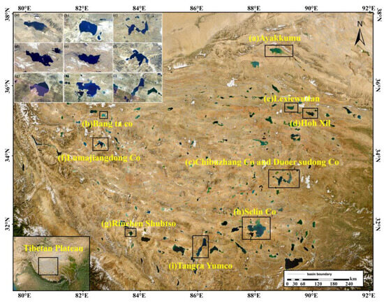
Figure 1.
Location of the study area and the distribution of the lakes.

Table 1.
Detailed information about the lakes and climatic factors.
2.2. Data
2.2.1. CMFD Data
The China meteorological forcing dataset (CMFD), developed by the Institute of Tibetan Plateau Research, Chinese Academy of Sciences, is the first reanalysis dataset with high spatial–temporal resolution and multi-meteorological elements to be used in land surface studies in China [32,33,34]. The comprehensive data of this dataset are a fusion of remote sensing products (GEWEX-SRB, GLDAS, and TRMM 3B42 precipitation datasets), Princeton reanalysis data, and meteorological observation data of the China Meteorological Administration. The dataset contains seven meteorological elements, including temperature, precipitation, wind speed, specific humidity, surface pressure, downward short-wave radiation, and downward long-wave radiation. The temporal and spatial resolution of this dataset are 3 h and 0.1° × 0.1°, respectively. The TP is characterized by complex topography and sparse meteorological stations, and CMFD has a strong interpretation ability of precipitation and temperature in high altitude and latitude regions. Therefore, this study used CMFD data to correct CMIP6 data. In order to verify the accuracy of CMIP6 data, the bilinear interpolation method was adopted to interpolate the resolution of CMFD data into 1° × 1°. The dataset is provided by the National Tibetan Plateau Data Center (http://data.tpdc.ac.cn, accessed on 13 January 2024).
2.2.2. CMIP6 Data
The data for precipitation, temperature, and evaporation in this study are monthly scale data from 20 climate models of CMIP6, and the basic data information is shown in Table 2. In order to reduce the data uncertainty effectively, this study adopts the multi-model ensemble average method, uniformly using the ensemble average values of 20 climate models for precipitation, temperature, and evaporation data. Among these, data from the historical context (1986~2014) were selected as the baseline period data, and the future scenario model of CMIP6 (SSP126, SSP245, SSP585, 2015~2100) was selected for future prediction research. SSP126, SSP245, and SSP585 represent the latest combination scenarios of the shared socio-economic path and typical concentration path of CMIP6, representing low forcing, medium forcing, and high forcing scenarios, respectively. Due to the varying resolutions of different climate models, the bilinear interpolation method was employed to interpolate the resolution into 1° × 1°. The dataset is provided by the World Climate Research Programme (https://esgf-node.llnl.gov/projects/cmip6/, accessed on 13 January 2024).

Table 2.
Basic information on the 20 models of the CMIP6 climate model.
2.2.3. Landsat Images and SRTM Data
Multi-temporal Landsat imagery was used to extract the lake surface boundary, with lake area calculated by using images with the minimum cloud and snow cover and the highest quality from September to November. Normalized Difference Water Index (NDWI) was used to extract the lake area. The equation of NDWI is expressed as:
where Green is the green band and NIR is the near-infrared band.
SRTM was used to obtain topography above the lake surface in 2000, enabling subsequent calculation of lake water storage change. SRTM, a joint project launched by NASA and the National Geospatial-Intelligence Agency in February 2000, involving collecting terrain data spanning from 60°N to 56°S over 11 days, using X-band and C-band Interferometric Synthetic Aperture radar sensors, accounts for about 80% of the world’s land terrain information. DEM data products are available in two spatial resolutions: 1 arcsecond and 3 arcseconds. SRTM-1 offers higher resolution and precision than SRTM-3. Therefore, this study selects one arc second resolution (30 m × 30 m) SRTM DEM data, which can be downloaded from CGIAR—CSI (http://srtm.csi.cgiar.org/, accessed on 13 January 2024).
3. Methods
3.1. Estimation of Lake Water Storage Changes
The boundary of the lake was extracted from Landsat images. Based on the topography above the lake surface in 2000 provided by SRTM, we established the relationship between lake area and lake level and estimated the change of lake water storage using an empirical equation with lake area data. This method has been widely used in the study of lake water storage change, with high accuracy, and the detailed method can be seen in Yang et al. [17] and Qiao et al. [13].
where S1 and S2 represent the lake area in different periods; ∆h is the lake level change; and ∆V is the lake water storage change. The lake area is obtained by Landsat images, and the water level data are estimated using SRTM and Landsat images.
3.2. Methodology for Correction of Precipitation Data Deviations
In this study, we compared the annual mean temperature and annual precipitation data from CMFD with those data from CMIP6 in the historical period (1986~2014), and the correlation coefficient of temperature was 0.95, while the precipitation data was 0.76 with a low correlation. In order to improve the accuracy of predicting future lake water storage changes, a deviation correction method based on frequency distribution (QM method) is adopted in this study to correct the CMIP6 precipitation data.
The method of QM considers that the frequency distribution of simulated and observed precipitation are consistent. If no assumptions are made about theoretical distribution followed by those data, this method is called Empirical Quantile Mapping (EQM). The method of EQM corrects the deviation of simulated precipitation data for future forecast periods by using percentiles, which calculates from uncorrected simulated precipitation data, and measured precipitation data for the base period. The specific methods are as follows:
- Cumulative distribution function (CDF). The observed and simulated precipitation data from 1986~2014 were sorted in ascending order and, using the precipitation series of the modeling time period with the following Formula (3), the cumulative probability density values of the simulated and observed values were calculated separately.
- 2.
- Non-parametric transformation QUANT: makes the empirical cumulative probability distribution function of the original output data as close as possible to the observations over the historical period:
We apply the established transfer function to future periods:
Thus, the revised data xbc are obtained. Among them, xh, Fcdfh, xf, and Fcdff are the model data and corresponding empirical CDF in the historical period and future period, respectively, and xo and Fcdfo are observed data and their corresponding empirical CDFs. The type of interpolation chosen among the fitted transfer values is a monotonic cubic spline interpolation method. The established transfer function is applied to the precipitation data for the future prognostic period, resulting in revised simulated data.
3.3. Random Forest Algorithm
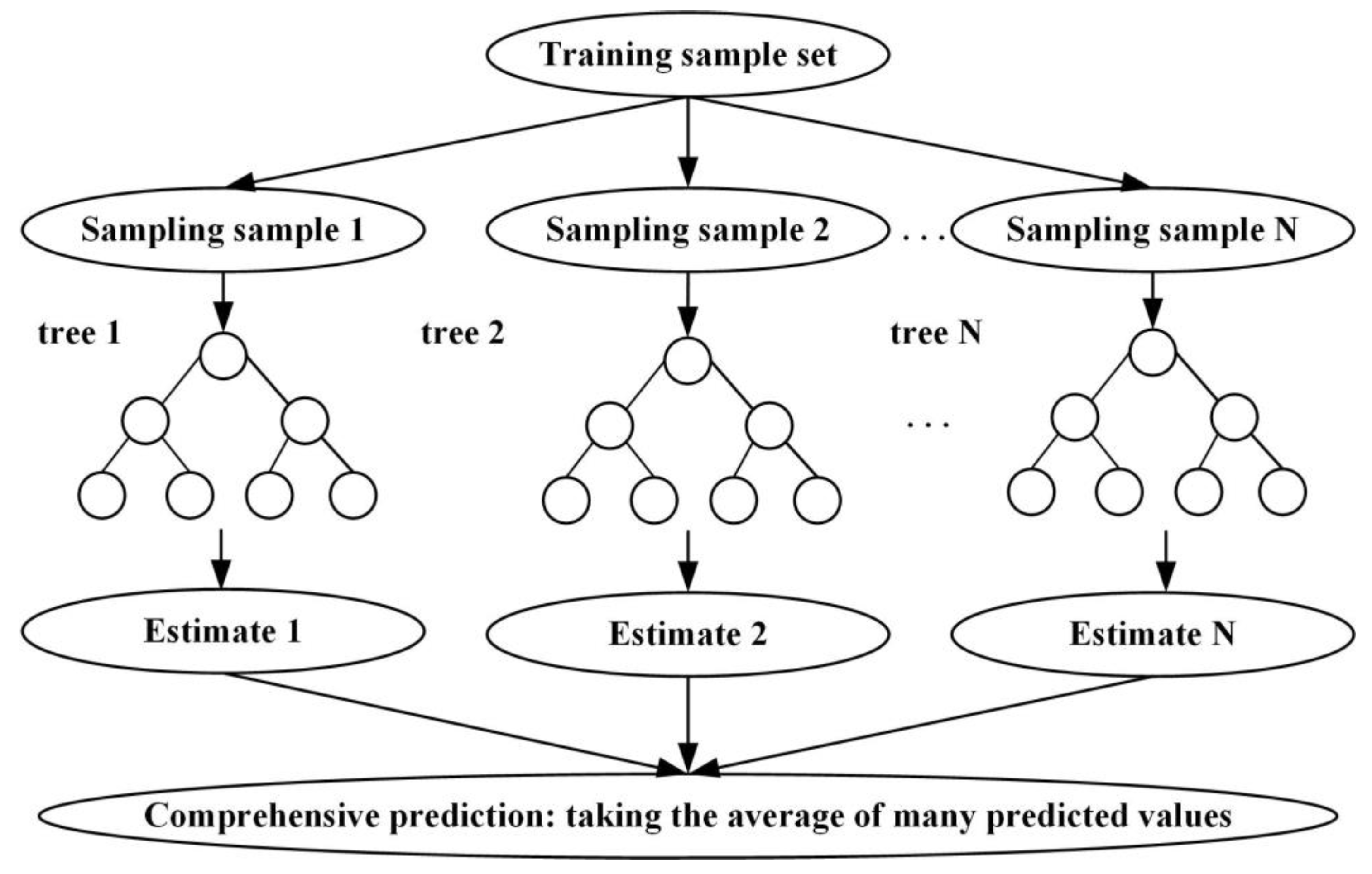
Random Forest (RF) is an integrated learning method proposed by Breiman in 2001 [35]. The algorithm is an integrated learning method based on the idea of Bagging integrating classification and regression, and RF combines the ideas of random subspace and decision tree to improve the performance of prediction. The working principle of RF is shown in Figure 2. First, several different types of mutually independent training sets are randomly selected from the sample data, and N training sets are selected as the root node samples of each regression tree to build the base decision tree. Then, during the tree construction process, a random feature subspace is selected at each node of the tree, and N decision trees are obtained with N results. These selected features are evaluated according to predefined criteria, Gini coefficients, and the optimal features are considered. Due to the randomization technique used in the algorithm, a diverse set of trees is created and the final prediction is made by combining the decisions of all the trees by averaging or voting.
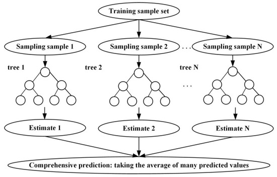
Figure 2.
Schematic diagram of RF.
3.4. Prediction Model
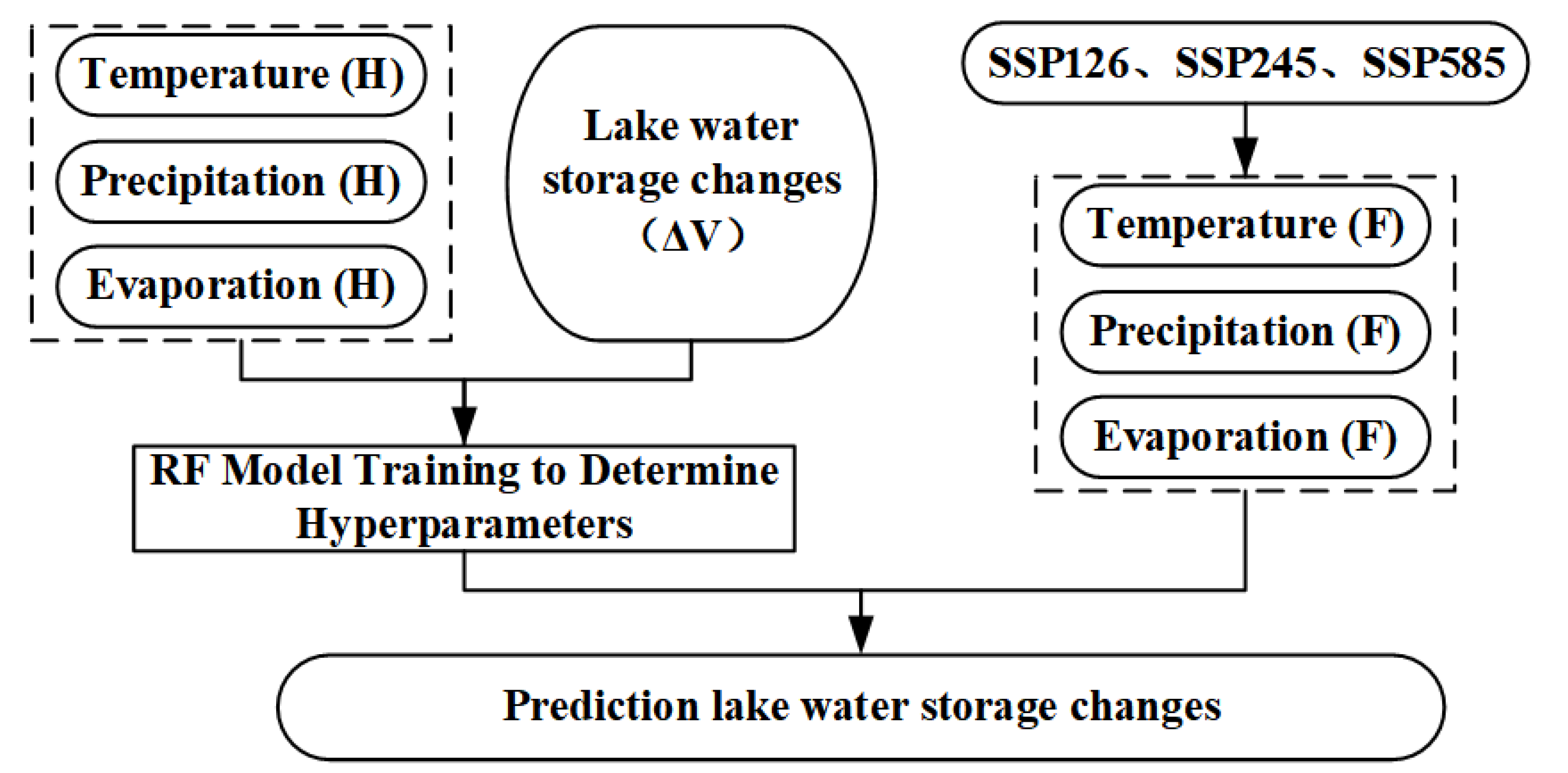
The basic idea of the RF model is to determine the factors that affect lake water storage changes, including annual precipitation, annual mean temperature, and annual evaporation. Firstly, to construct the RF regression model, the tuning of the model is performed to determine the optimal parameters of the model, and finally, the input of future meteorological data (CMIP6) is used to apply the prediction model to predict the future lake water storage change. The basic process is shown in Figure 3.
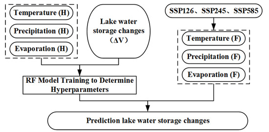
Figure 3.
Flow chart of RF modeling (H for historical period, F for future period).
The data of the annual lake water storage change, annual precipitation, annual mean temperature, and annual evaporation during 1986~2014 are selected as the model sample set, among which the ratio of training set to test set was 7:3. After the training set is determined, the model was carried out. During the modeling process, the RF performance super parameters are determined as n_estimators, max_depth, and max_features. n_estimators represent the maximum number of iterations of the weak learner, namely the number of trees. The number of decision trees determines the stability of the predicted results. Therefore, to some extent, the larger the number of decision trees, the better. There are little data in this experiment, so it is unnecessary to deliberately limit the depth of the decision tree. However, in general, the smaller the tree depth, the smaller the calculation amount and the faster the running speed. Max_features represents the maximum number of features involved in the judgment when the node is split, and the number of feature attributes in this experiment is 3. The experimental data storage is small, so the traversal method is adopted to determine the optimal parameters. The specific steps are as follows:
Step 1: Set the range of the number of decision trees as [1, 250]; the maximum depth range is [1, 20].
Step 2: Set the step size of the optimization parameter for the number of decision trees to 1 and the step size of the optimization parameter for the maximum depth of the decision tree to 1.
Step 3: By adjusting the parameters, R2, MAE, and RMSE of the training set and test set were calculated, respectively, and the optimal parameters of the model were determined by comparing the evaluation criteria. The calculation formula of R2, MAE, and RMSE is as follows:
In the formula, n is the number of samples; Yi is the real value of water storage change in the ith lake; is the predicting value calculated by the ith RF model; is the mean value of the real value.
By traversing parameters for tuning, a total of 500 parameter combinations are obtained. By comparing the metrics of each parameter combination, the optimal parameters of each lake are finally determined, as shown in Table 3.

Table 3.
Hyperparameter values of each lake.
3.5. Accuracy Assessment
3.5.1. Model Accuracy
In this study, R2 (Correlation Coefficient), MAE (Mean Absolute Error), and RMSE (Root Mean Square Error) are used as evaluation indexes of the model to analyze the performance of the prediction model of lake water storage change based on random forest regression. R2 evaluated the consistency between the predicted value of lake water storage change and the real value. The closer R2 is to 1, the more stable the model is and the better the fitting effect is. RMSE represents the predictive power of the model.
3.5.2. Computational Uncertainty
We calculate the Standard Error (SE) of annual mean temperature, annual precipitation, and evaporation from 20 CMIP6 models, and assess the uncertainty of lake water storage change prediction with SE. For example, we add SE or subtract SE to precipitation, temperature, and evaporation, and then calculate the change of lake water storage, and consider the largest uncertainly of those results as the uncertainly of annual lake water storage prediction. Through this approach, we comprehensively consider uncertainty factors, enhancing the reliability of lake water storage change predictions. The calculation formula of SE is as follows:
δ represents the standard deviation of temperature, precipitation, and evaporation data from 20 CMIP6 models, n is the sample number.
4. Results
4.1. Deviation Correction Results of Precipitation Data
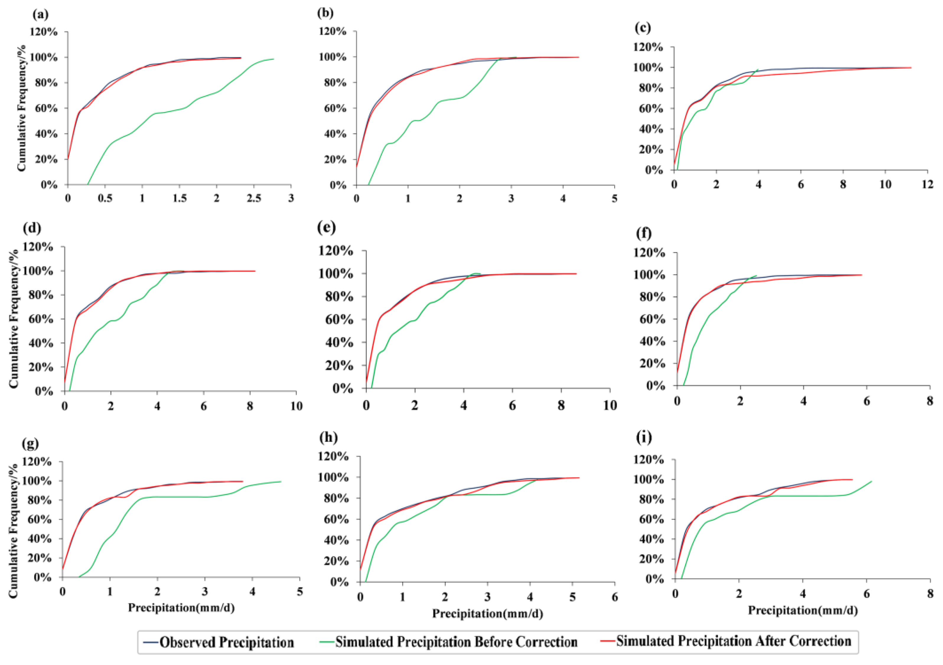
As shown in Figure 4, an analysis of the frequency cumulative distribution diagram (CDF) for each lake reveals that the precipitation with a cumulative frequency of CMFD within 97% of each lake falls within the range of 0~4 mm. Among these lakes, the simulated precipitation data for CD, RC, and TY were distributed from 0 to 6 mm/d, whereas the simulated precipitation data for AK, BD, HX, LX, LM, and SL were distributed from 0 to 4 mm/d. By comparing the CDF curves of simulated precipitation data before and after correction with observed precipitation data, it can be observed that the CDF curve of simulated precipitation before correction for AK, BD, HX, LX, LM, and RC exhibits a significant deviation from observed precipitation, with the majority of this discrepancy concentrated within 97% of the cumulative frequency range. The difference arises primarily due to the fact that small- and medium-sized precipitation accounts for a larger proportion of total precipitation relative to extreme precipitation events in the simulated precipitation data. Application of the QM method to correct simulated precipitation data leads to a closer alignment of the cumulative frequency distribution curve of observed precipitation and corrected precipitation in CMIP6. The large amount of wet bias (difference from observed precipitation greater than zero) observed in precipitation events with a cumulative frequency less than 97% is significantly reduced following QM correction. The deviation between simulated and observed precipitation curves before CD, SL, and TY correction is relatively small, especially for CD, where the CDF curve of simulated precipitation aligns closely with the CMFD curve. After QM correction, the coincidence rate between CDF curves corrected using CMFD and CMIP6 is within 0.9.
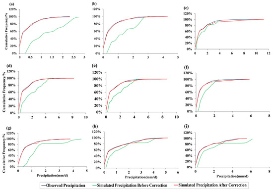
Figure 4.
Frequency cumulative distribution of the lake basins. (a) AY; (b) BD; (c) CD; (d) HX; (e) LX; (f) LM; (g) RC; (h) SL; (i) TY.
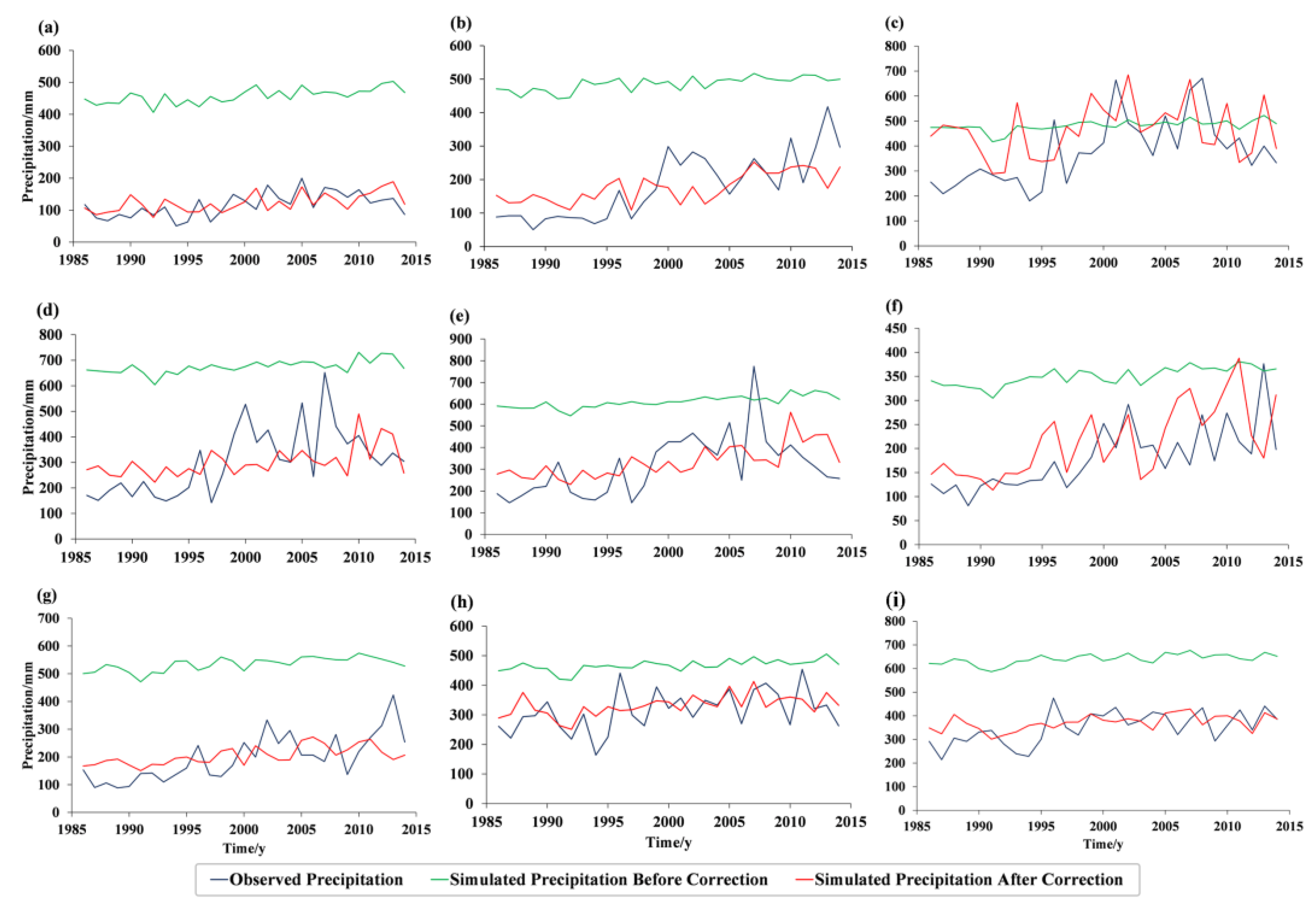
Figure 5 shows the distribution of the annual total precipitation of the nine lakes, and it is evident that a significant difference exists between the annual precipitation of the observed data and that of the simulated data before correction, with precipitation being overestimated to different degrees. The simulated annual precipitation prior to correction is around 1.5~2 times the value of the observed annual precipitation. Following QM correction, a substantial reduction in the deviation is observed when comparing the annual precipitation of each lake to that of the observed annual precipitation. The annual value of observed precipitation, simulated precipitation before correction, and simulated precipitation after correction of each lake are shown in Table 4. The annual precipitation deviation of AY, BD, HX, and RC decreased from 341.11 mm, 306.60 mm, 370.82 mm, and 337.17 mm to 6.83 mm, −3.74 mm, −3.38 mm, and 7.65 mm, respectively. The annual precipitation deviation was constrained within ±10 mm, indicating a more pronounced correction effect. As the precipitation correction data by QM rely on frequency distribution, the correction effect in numerical terms is generally moderate. The correlation coefficient between CMFD precipitation and corrected CMIP6 precipitation of each lake after QM correction is lower than that between CMFD precipitation and CMIP6 precipitation, and the reduction in the correlation coefficient is maintained below 0.09.
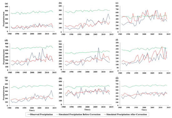
Figure 5.
Comparison of observed precipitation and simulated precipitation. (a) AY; (b) BD; (c) CD; (d) HX; (e) LX; (f) LM; (g) RC; (h) SL; (i) TY.

Table 4.
Correlation coefficients between observed precipitation and simulated precipitation in each lake before and after correction.
4.2. Model Accuracy Assessment
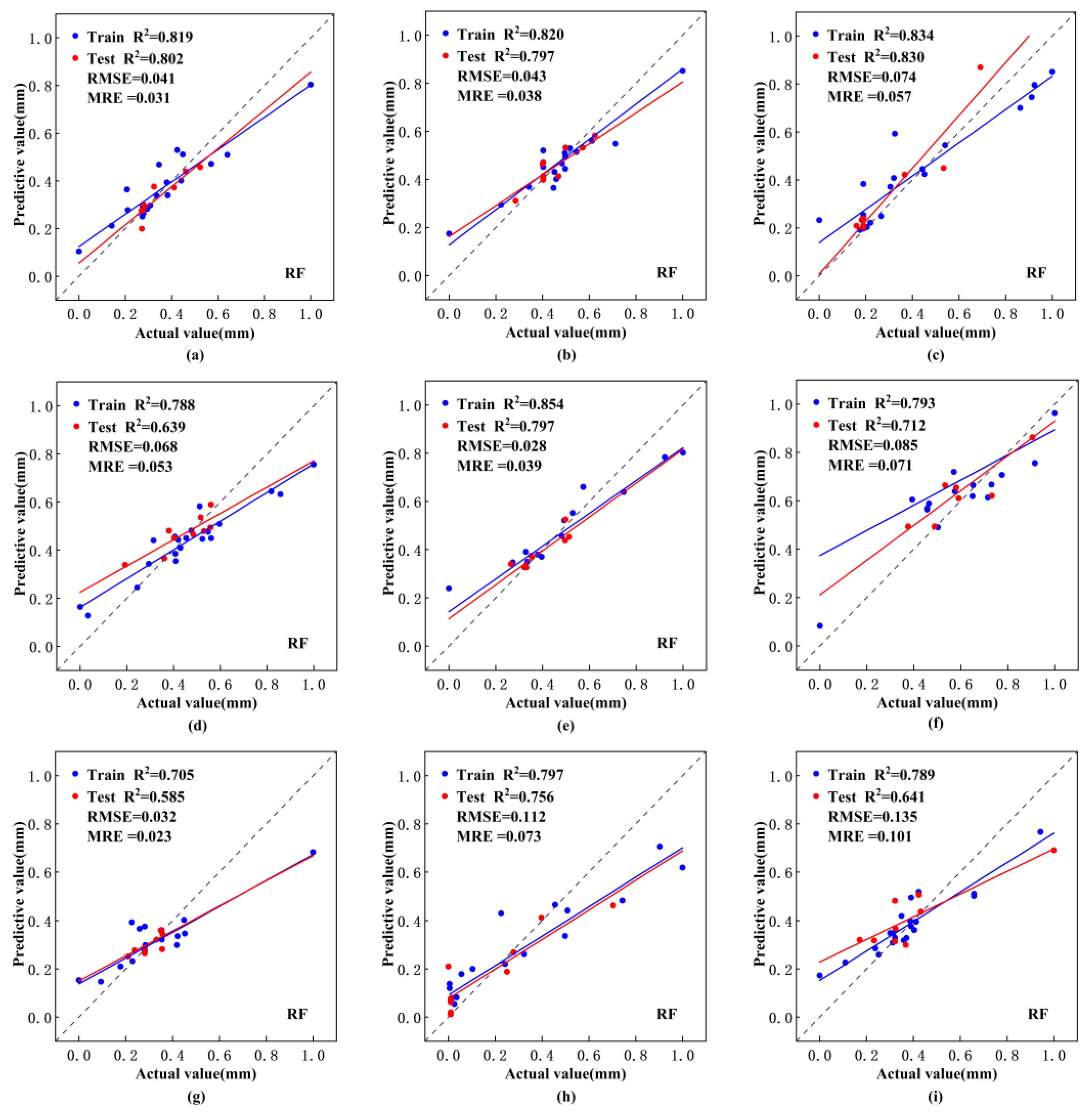
Based on the data from the historical periods, including lake water storage change, annual mean temperature, annual precipitation, and annual evaporation, we built RF models for predicting lake water storage change. Figure 6 presents the data and results of lake water storage change by the test set and training set of the RF model. The scatter plot shows the predicted lake water storage change from the RF prediction model compared to the actual value. The fitting line for the training and test sets of AK, BD, HX, LX, LM, and TY closely follow the 1:1 line, indicating good model performance. However, RC and SL lakes have fewer sample points in the low-value precipitation range, causing their fitting line to deviate more from the 1:1 line. LM lake demonstrates weaker performance due to sparse data points in the high-value precipitation area, resulting in a scattered point distribution and a large offset angle for the fitting line.
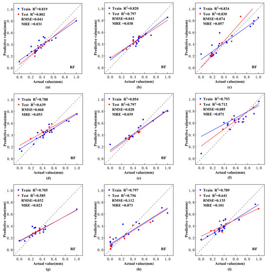
Figure 6.
Scatter plot of lake water storage inversion with test set and training set. (a) AY; (b) BD; (c) CD; (d) HX; (e) LX; (f) LM; (g) RC; (h) SL; (i) TY.
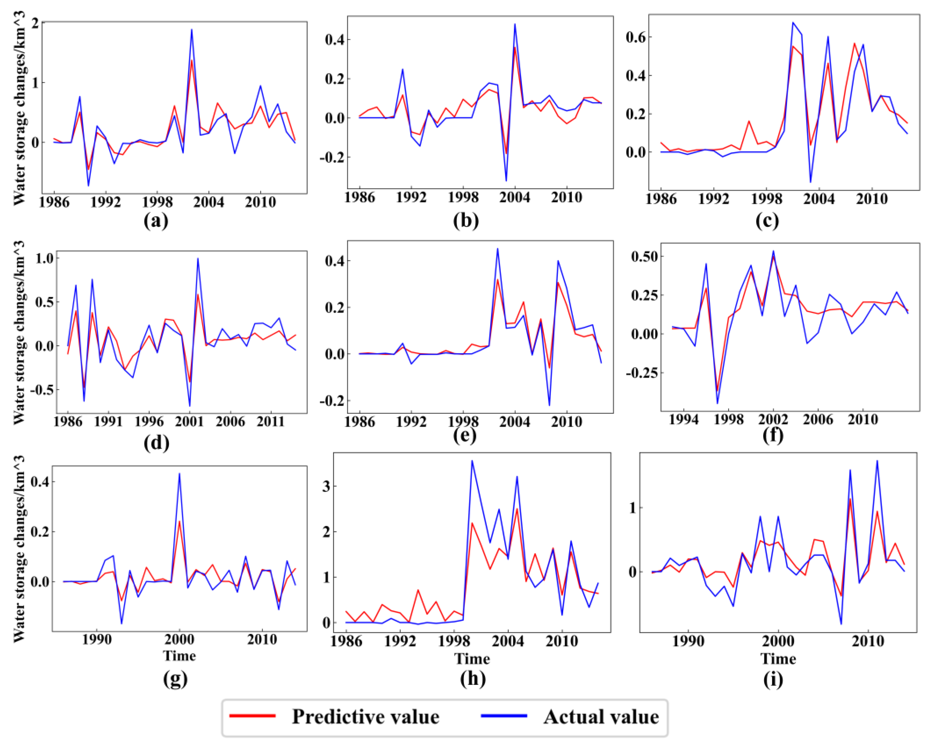
The accuracy of the RF model was evaluated by analyzing the performance of the test set for each lake. Table 5 represents the results. The CF lake with an R2 of 0.830 and RMSE of 0.074 km3 exhibits the best training effect among the nine lakes. The RC lake shows the greater error, with an RMSE of 0.039 km3 and an R2 of 0.585 for test, and an RMSE of 0.105 km3 for training. The RMSE of the AK, BD, CD, HX, LX, LM, and RC test sets were all less than 0.1 km3, while these for SL and TY lakes were slightly higher, at 0.112 km3 and 0.135 km3, respectively. In addition, the R2 of the model training set was consistently higher than the corresponding test sets. The MAE and RMSE of the training set are lower than those of the test set, confirming the model’s overall good accuracy. Figure 7 illustrates some deviations between the predicted and observed values of lake water storage change during the historical periods, but the overall trend of lake water storage change trend is well-represented by the model.

Table 5.
Precision evaluation parameters of RF models in each lake.
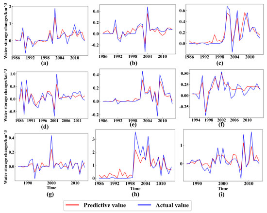
Figure 7.
Comparison of predictive and actual lake water storage change in historical period. (a) AY; (b) BD; (c) CD; (d) HX; (e) LX; (f) LM; (g) RC; (h) SL; (i) TY.
4.3. Prediction of Lake Water Storage Changes under Different SSP Scenarios
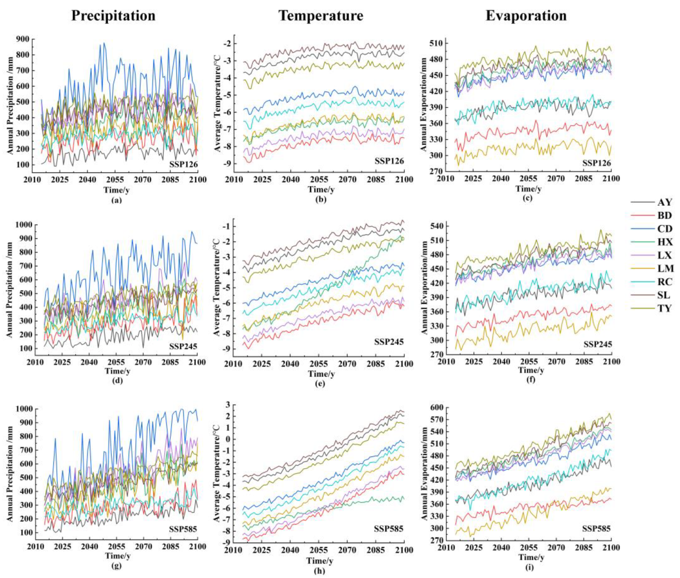
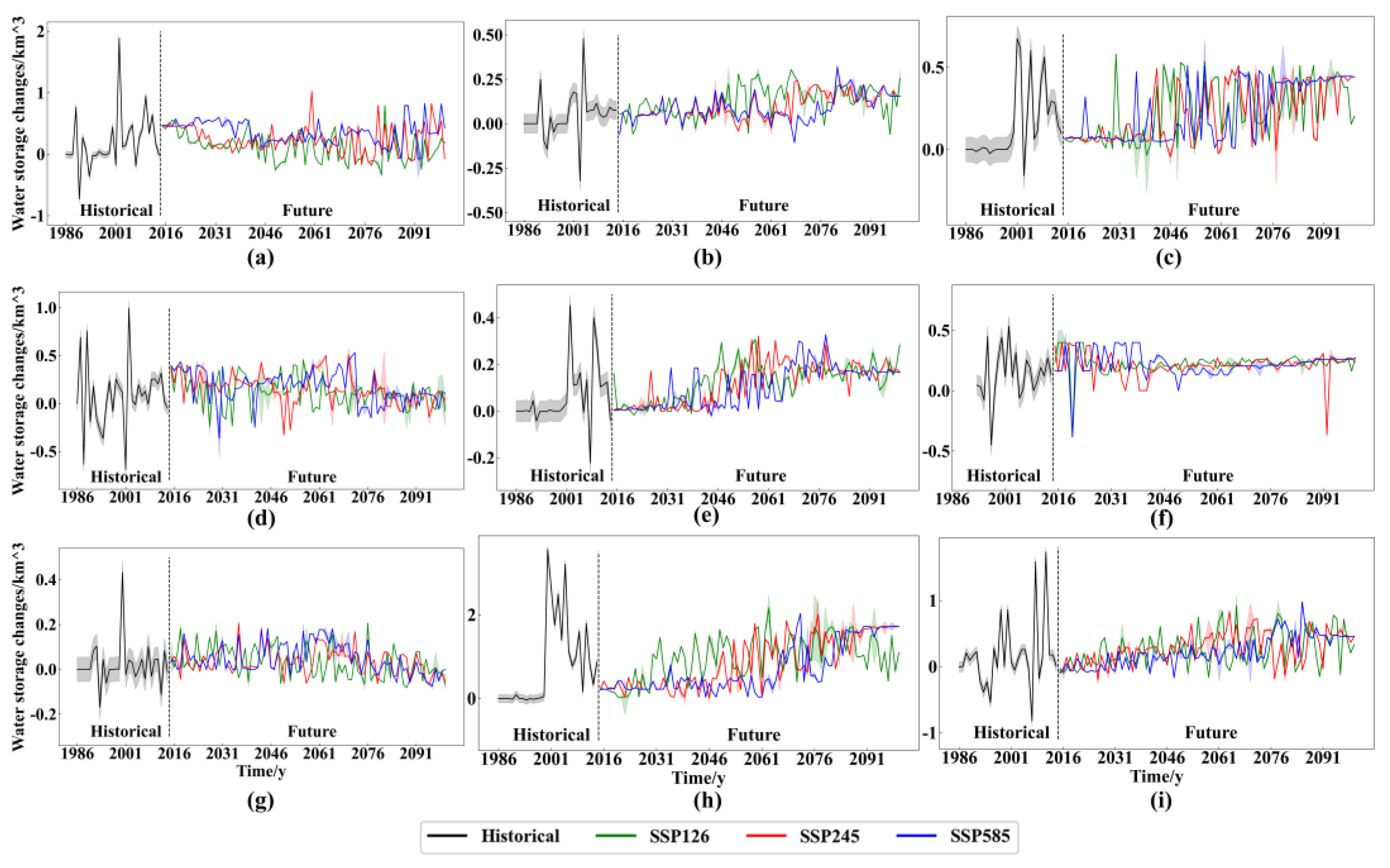
RF prediction model is used to predict the future water storage changes in nine lakes based on projected data for precipitation (Figure 8a,d,g), temperature (Figure 8b,e,h), and evaporation (Figure 8c,f,i) under three scenarios. A gradual increasing trend in the temperature, precipitation, and evapotranspiration under the three scenarios is noticed. The prediction of lake water storage changes are shown in Figure 9. Figure 9 shows the historical (1986~2014) and future (2015~2100) trends of annual lake water storage under three scenarios. Most lakes exhibit considerable variation in their annual lake water storage change, especially CD. Most of them show an increasing trend. The increasing rate of HX and RC slows after 2070, and the latter has a shrinkage trend. Even though BD, CD, and LX have an increasing trend, their predictions have a larger uncertainly than other lakes.

Figure 8.
The changing trends of temperature, precipitation, and evaporation in nine lakes basins under the three scenarios from 2015 to 2100. (a,d,g) represent precipitation in the three scenarios, respectively, (b,e,h) represent temperature in the three scenarios, respectively, (c,f,i) represent evaporation in the three scenarios, respectively. SSP126 represents the low carbon emission scenario, SSP245 represents the medium carbon emission scenario, and SSP585 represents the high carbon emission scenario.
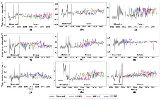
Figure 9.
Interannual changes in lake water storage predicted by the historical period (1986~2014) and the future period (2015~2100). (a) AY; (b) BD; (c) CD; (d) HX; (e) LX; (f) LM; (g) RC; (h) SL; (i) TY.
4.4. Future Changes of Lake Water Storage
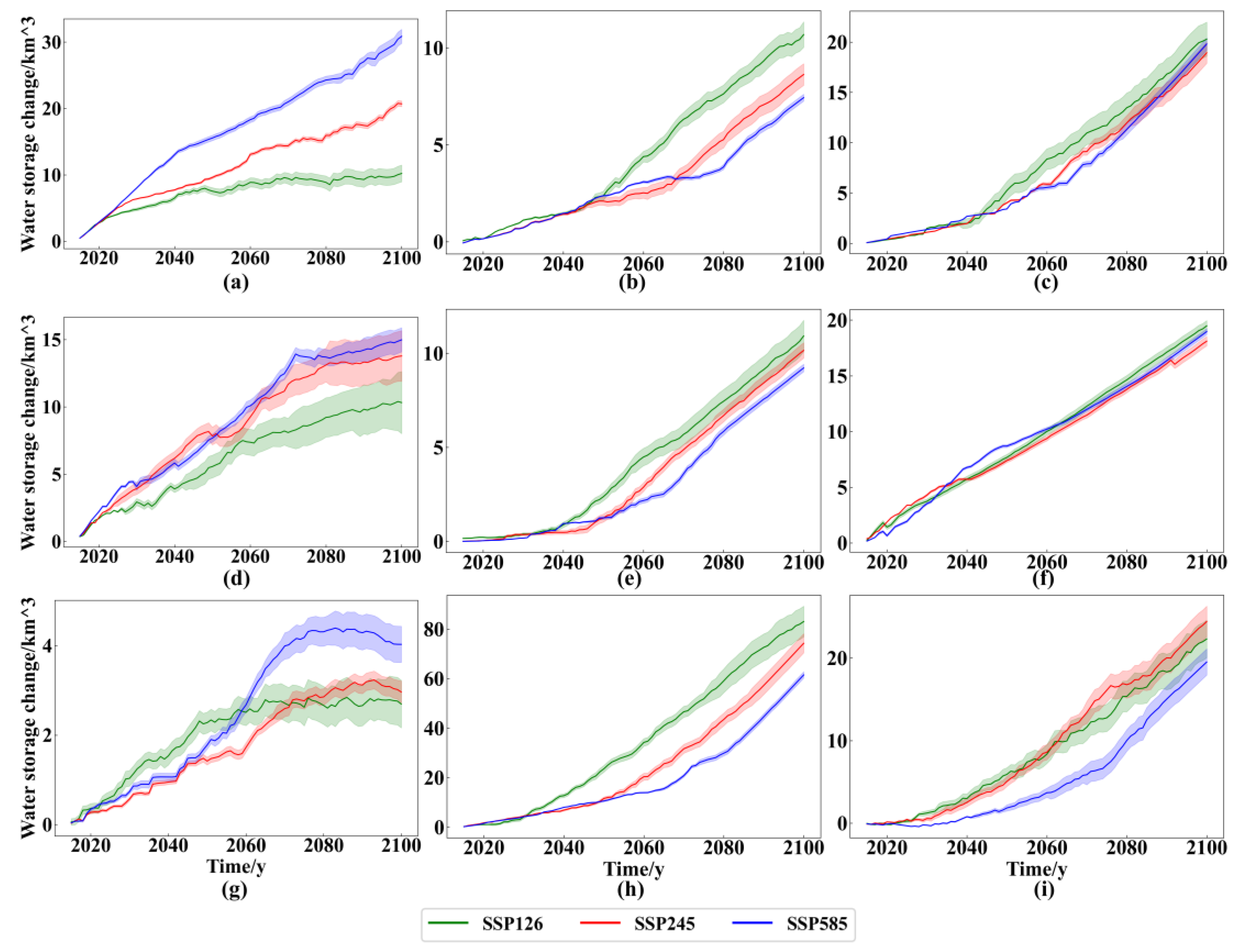
The future water storage changes are shown in Figure 10 and Table 6. Large differences exist between different scenarios, with most lakes demonstrating a quick increase in water storage under three scenarios. By 2100, the total water storage of the nine lakes is projected to increase by 189.676 ± 16.266 km3, 191.762 ± 10.683 km3, and 186.212 ± 6.441 km3 until 2100 under the SSP126, SSP245, and SSP585 scenarios, respectively. However, the increasing rate varies substantially across scenarios and lakes. For example, the increasing rate under SSP585 in AY and HX is larger than in other scenarios, but the increasing rate under SSP126 in BC, LX, and SL is the largest among those scenarios. The increase in CD and LM remains relatively consistent across all three scenarios.
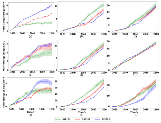
Figure 10.
Future trends of lake water storage change. (a) AY; (b) BD; (c) CD; (d) HX; (e) LX; (f) LM; (g) RC; (h) SL; (i) TY.

Table 6.
Future changes of lake water storage in each lake.
Lake water storage of AY, HX, and RC showed a quick initial increasing trend, followed by a slow increase. The lake water storage of AY under the three scenarios remains relatively stable during 2015–2020, within a range of about 5%. However, after 2020, the increasing rate under SSP126 declined sharply, while under the SSP245 and SSP585 scenarios, it continues to increase quickly. The increasing rate of AY is 0.236 ± 0.014 km3/y during 2015–2050 and 0.196 ± 0.005 km3/y during 2051~2100 under SSP245.
The variation trend of lake water storage in HX under the three scenarios is similar during 2015~2025, but the SSP126 scenario shows a relatively stable trend, while the SSP245 scenario exhibits more drastic fluctuations than that of the other two scenarios. After 2025, the variation trends of lake water storage under the three scenarios begin to diverge. The lake water storage under SSP126 gradually increased at a low rate, and SSP245 and 585 exhibit similar but faster increases until 2075, followed by a slowdown under all three scenarios. As shown in Table 6, the average annual increase rate for HX is 0.19 ± 0.015 km3/y during 2015~2060 and 0.093 ± 0.003 km3/y during 2061~2100 under SSP245. RC experiences a relatively low increase rate, with 0.04 ± 0.002 km3/y during 2015~2060 and 0.028 ± 0.003 km3/y during 2061~2100 under SSP245.
The water storage change of BD, CD, LX, SL, and TY has a little and similar changing rate in all three scenarios until 2030 or 2040, and then expands quickly with different changing rates. The increasing rate under SSP585 is the smallest, while SSP126 shows the largest, except for TY, which sees the most expansion under the SSP245 scenario. Within the scenario of SSP245, SL shows the largest expansion, exhibiting a quick increase of 1.268 ± 0.065 km3/y during 2051~2100, followed by TY, with 0.357 ± 0.002 km3/y during 2031~2100.
5. Discussion
Due to there is a large difference between observed precipitation (CMFD) and simulated precipitation (CMIP6) before correction, and the simulated precipitation prior to correction is around 1.5~2 times the observed precipitation. Therefore, a suitable correction method is necessary to correct the data of precipitation. In this study, we used the QM method to correct the precipitation data, and a substantial reduction in the deviation is observed after QM correction when comparing with the observed annual precipitation. However, at the same time, the overcorrection occurs during the correction process for each lake, meaning that the simulated data deviate even further from the observed value after correction. The main reason is that the annual precipitation for each lake is relatively small, with precipitation mainly concentrated in the low-value range. During the construction of the transfer function, the partial precipitation data less than 0.97 fall within a 0~4 mm/d range, with more sample points concentrating in this range, resulting in a relatively stable constructed transfer function. However, during the construction of the trans-fer function for extreme precipitation (4~9 mm/d), there are fewer sample points. The fitting degree of the function is low with poor stability, leading to a poor simulation effect for high-value precipitation after correction.
We also assess the accuracy of prediction model based on RF, and the results showed that most of those points were close to the line 1:1, and the CF lake exhibits the best result (R2 of 0.830 and RMSE of 0.074 km3) among the nine lakes. The RMSE of most lakes was less than 0.1 km3, only SL and TY lakes were slightly higher with 0.112 km3 and 0.135 km3, respectively. Therefore, the prediction model performed with a good accuracy, and we used the model to predict the lake water storage change in the future. Under the three scenarios, even though most of those lakes have an increasing trend, there is a large variation for annual water storage change. Especially for LM, which expands quickly with a relatively stable increasing trend. This fact is attributable to the dominant influence of precipitation on the change of lake water storage. Analysis of the relationship between annual precipitation and lake water storage change reveals that periods of abrupt change in 1997, 2020, and 2092 coincide with significantly lower precipitation levels. As shown in Table 6, the increasing rate under three scenarios is consistent with 0.188 ± 0.005 km3/y during 2015~2050 and 0.216 ± 0.005 km3/y during 2050~2100 under SSP245, and the total water storage will increase by 19.486 ± 0.473 km3, 18.107 ± 0.417 km3, and 18.969 ± 0.265 km3 until 2100 under three scenarios of SSP126, SSP245, and SSP585, respectively.
6. Conclusions
In this study, we estimated the annual change of lake water storage from 1986 to 2014 using Landsat and SRTM data and established a prediction model that combines RF models with historical climate factors. We then used the prediction model to estimate the annual change of lake water storage under different carbon emission scenarios in the next 80 years using CMIP6 data. The key findings are as follows:
- (1)
- The correlation coefficients between CMFD and models derived from 20 CMIP6 temperature datasets in the historical period are more than 0.9, and the correlation coefficients for precipitation are 0.7. We used the QM method to correct precipitation data, resulting in a close match between corrected CMIP6 precipitation data and CMFD precipitation data in terms of frequency.
- (2)
- The RF model exhibited a strong performance in predicting historical water storage changes. The R2 values for the training and the testing sets of the nine lakes are greater than 0.7 and 0.6, and the MAE for most lakes was less than 0.1 km3. This indicates that the model accurately captured the relationship between historical water storage changes and climate factors.
- (3)
- Under the three future SSP scenarios, the temperature, precipitation, and evaporation of the nine lakes are projected to increase, leading to an expansion in lake water storage. For AY, HX, and RC, there is an initial rapid increase followed by a gradual decrease or stabilization; BD, CD, LX, SL, and TY exhibit an initial slow increase followed by a rapid increase; LM maintains a steady increase, and the rate of increase is consistent across the three scenarios.
- (4)
- The increasing rate under SSP585 in AY and HX is greater than in other scenarios, but the increasing rate under SSP126 in BD, LX, and SL is the largest among those scenarios. The increasing rates of CD and LM are consistent across the three scenarios.
- (5)
- SL is projected to experience the largest expansion, with an annual increase of 1.268 ± 0.065 km3/y during 2051~2100, followed by TY with 0.357 ± 0.002 km3/y. RC is projected to show little or no increase after 2050. The total water storage of the nine lakes will increase by 189.676 ± 16.266 km3, 191.762 ± 10.683 km3, and 186.212 ± 6.441 km3 until 2100 under the SSP126, SSP245, and SSP585 scenarios, respectively.
Author Contributions
Conceptualization, Y.H., B.Q. and L.Z.; methodology, Y.H., B.Q. and L.Z.; software, Y.H.; validation, Y.H. and B.Q.; formal analysis, Y.H.; investigation, Y.H. and R.Z.; resources, B.Q. and L.Z.; data curation, B.Q. and L.Z.; writing—original draft preparation, Y.H.; writing—review and editing, Y.H., B.Q., R.Z. and L.Z.; visualization, Y.H.; supervision, B.Q. and L.Z.; funding acquisition, B.Q. and L.Z. All authors have read and agreed to the published version of the manuscript.
Funding
This work was supported by the Second Tibetan Plateau Scientific Expedition and Research (2019QZKK0202), NSFC project (41831177, 41901078).
Data Availability Statement
Publicly available datasets were analyzed in this study. CMFD data can be found here: https://doi.org/10.11888/AtmosphericPhysics.tpe.249369.file (accessed on 13 January 2024); CMIP6 data can be found here: https://esgf-node.llnl.gov/projects/cmip6/ (accessed on 13 January 2024); SRTM data can be found here: http://srtm.csi.cgiar.org/ (accessed on 13 January 2024).
Conflicts of Interest
The authors declare that they have no known competing financial interests or personal relationships that could have appeared to influence the work reported in this paper.
References
- Montanari, A.; Young, G.; Savenije, H.H.G.; Hughes, D.; Wagener, T.; Ren, L.L.; Koutsoyiannis, D.; Cudennec, C.; Toth, E.; Grimaldi, S.; et al. “Panta Rhei—Everything flows”: Change in hydrology and society—The IAHS scientific decade 2013–2022. Hydrol. Sci. J. 2013, 58, 1256–1275. [Google Scholar] [CrossRef]
- Berghuijs, W.R.; Woods, R.A.; Hrachowitz, M. A precipitation shift from snow towards rain leads to a decrease in streamflow. Nat. Clim. Change 2014, 4, 583–586. [Google Scholar] [CrossRef]
- Climate Change 2013: The Physical Science Basis: Working Group I Contribution to the Fifth Assessment Report of the Intergovernmental Panel on Climate Change; Cambridge University Press: Cambridge, UK, 2014.
- Climate Change 2021: The Physical Science Basis. Contribution of Working Group14 I to the Sixth Assessment Report of the Intergovernmental Panel on Climate Change; Technical Summary; The Intergovernmental Panel on Climate Change: Geneva, Switzerland, 2021.
- Xu, Z.X.; Gong, T.L.; Li, J.Y. Decadal trend of climate in the Tibetan Plateau—Regional temperature and precipitation. Hydrol. Process. Int. J. 2008, 22, 3056–3065. [Google Scholar] [CrossRef]
- Wan, W.; Xiao, P.; Feng, X.; Li, H.; Ma, R.; Duan, H.; Zhao, L. Monitoring lake changes of Qinghai-Tibetan Plateau over the past 30 years using satellite remote sensing data. Chin. Sci. Bull. 2014, 59, 1021–1035. [Google Scholar] [CrossRef]
- Zhang, G.; Yao, T.; Xie, H.; Zhang, K.; Zhu, F. Lakes’ state and abundance across the Tibetan Plateau. Chin. Sci. Bull. 2014, 59, 3010–3021. [Google Scholar] [CrossRef]
- Zhang, G.; Yao, T.; Xie, H.; Wang, W.; Yang, W. An inventory of glacial lakes in the Third Pole region and their changes in response to global warming. Glob. Planet. Change 2015, 131, 148–157. [Google Scholar] [CrossRef]
- Phan, V.H.; Lindenbergh, R.; Menenti, M. ICESat derived elevation changes of Tibetan lakes between 2003 and 2009. Int. J. Appl. Earth Obs. Geoinf. 2012, 17, 12–22. [Google Scholar] [CrossRef]
- Song, C.; Huang, B.; Ke, L.; Richards, K.S. Seasonal and abrupt changes in the water level of closed lakes on the Tibetan Plateau and implications for climate impacts. J. Hydrol. 2014, 514, 131–144. [Google Scholar] [CrossRef]
- Zhang, G.; Xie, H.; Kang, S.; Yi, D.; Ackley, S.F. Monitoring lake level changes on the Tibetan Plateau using ICESat altimetry data (2003–2009). Remote Sens. Environ. 2011, 115, 1733–1742. [Google Scholar] [CrossRef]
- Zhu, L.; Zhang, G.; Yang, R.; Liu, C.; Yang, K.; Qiao, B.; Han, B. Lake variations on Tibetan Plateau of recent 40 years and future changing tendency. Bull. Chin. Acad. Sci. 2019, 34, 1254–1263. [Google Scholar] [CrossRef]
- Qiao, B.; Zhu, L.; Yang, R. Temporal-spatial differences in lake water storage changes and their links to climate change throughout the Tibetan Plateau. Remote Sens. Environ. 2019, 222, 232–243. [Google Scholar] [CrossRef]
- Song, C.; Huang, B.; Ke, L. Modeling and analysis of lake water storage changes on the Tibetan Plateau using multi-mission satellite data. Remote Sens. Environ. 2013, 135, 25–35. [Google Scholar] [CrossRef]
- Zhang, G.; Luo, W.; Chen, W.; Zheng, G. A robust but variable lake expansion on the Tibetan Plateau. Sci. Bull. 2019, 64, 1306–1309. [Google Scholar] [CrossRef] [PubMed]
- Zhang, G.; Chen, W.; Xie, H. Tibetan Plateau’s lake level and storage changes from NASA’s ICESat/ICESat-2 and Landsat missions. Geophys. Res. Lett. 2019, 46, 13115–13116. [Google Scholar] [CrossRef]
- Yang, R.; Zhu, L.; Wang, J.; Ju, J.; Ma, Q.; Turner, F.; Guo, Y. Spatiotemporal variations in storage of closed lakes on the Tibetan Plateau and their climatic responses from 1976 to 2013. Clim. Change 2017, 140, 621–633. [Google Scholar] [CrossRef]
- Yao, F.; Wang, J.; Yang, K.; Wang, C.; Walter, B.A.; Crétaux, J.-F. Lake storage variation on the endorheic Tibetan Plateau and its attribution to climate change since the new millennium. Environ. Res. Lett. 2018, 13, 064011. [Google Scholar] [CrossRef]
- Zhang, G.; Yao, T.; Shum, C.K.; Yi, S.; Yang, K.; Xie, H.; Feng, W.; Bolch, T.; Wang, L.; Behrangi, A.; et al. Lake volume and groundwater storage variations in Tibetan Plateau’s endorheic basin. Geophys. Res. Lett. 2017, 44, 5550–5560. [Google Scholar] [CrossRef]
- Zhang, X.Q.; Peng, L.L.; Lin, Z.H. Progress on the projections of future climate change with various emission scenarios. Adv. Earth Sci. 2008, 23, 174–185. [Google Scholar]
- Zhou, T.; Chen, Z.; Zou, L.; Chen, X.; Yu, Y.; Wang, B.; Bao, Q.; Bao, Y.; Cao, J.; He, B.; et al. Development of climate and earth system models in China: Past achievements and new CMIP6 results. J. Meteorol. Res. 2020, 34, 1–19. [Google Scholar] [CrossRef]
- Eyring, V.; Cox, P.M.; Flato, G.M.; Gleckler, P.J.; Abramowitz, G.; Caldwell, P.; Collins, W.D.; Gier, B.K.; Hall, A.D.; Hoffman, F.M.; et al. Taking climate model evaluation to the next level. Nat. Clim. Change 2019, 9, 102–110. [Google Scholar] [CrossRef]
- Zhang, B.; Dai, X.G. Assessment of the deviation of China precipitation projected by CMIP5 models for 2006–2013. Chin. J. Atmos. Sci. 2016, 40, 981–994. [Google Scholar]
- Huang, X.; Le, Q.; Zhang, M. Future precipitation change in the Belt and Road Region under representative concentration Pathway Scenarios. J. Yangtze River Sci. Res. Inst. 2020, 37, 53–60. [Google Scholar]
- Kraaijenbrink, P.D.; Stigter, E.E.; Yao, T.; Immerzeel, W.W. Climate change decisive for Asia’s snow meltwater supply. Nat. Clim. Change 2021, 11, 591–597. [Google Scholar] [CrossRef]
- Lun, Y.; Liu, L.; Cheng, L.; Li, X.; Li, H.; Xu, Z. Assessment of GCMs simulation performance for precipitation and temperature from CMIP5 to CMIP6 over the Tibetan Plateau. Int. J. Clim. 2021, 41, 3994–4018. [Google Scholar] [CrossRef]
- Xu, X.; Wu, Q. Active Layer thickness variation on the Qinghai-Tibetan Plateau: Historical and projected trends. J. Geophys. Res. Atmos. 2021, 126, e2021JD034841. [Google Scholar] [CrossRef]
- Yin, G.A.; Niu, F.J.; Lin, Z.J.; Luo, J.; Liu, M.H. Data-driven spatiotemporal projections of shallow permafrost based on CMIP6 across the Qinghai–Tibet Plateau at 1 km2 scale. Adv. Clim. Change Res. 2021, 12, 814–827. [Google Scholar] [CrossRef]
- Wang, T.; Zhao, Y.; Xu, C.; Ciais, P.; Liu, D.; Yang, H.; Piao, S.; Yao, T. Atmospheric dynamic constraints on Tibetan Plateau freshwater under Paris climate targets. Nat. Clim. Change 2021, 11, 219–225. [Google Scholar] [CrossRef]
- Amengual, A.; Homar, V.; Romero, R.; Alonso, S.; Ramis, C. A Statistical adjustment of regional climate model outputs to local scales: Application to Platja de Palma, Spain. J. Clim. 2012, 25, 939–957. [Google Scholar] [CrossRef]
- Anderson, B.; Mackintosh, A. Controls on mass balance sensitivity of maritime glaciers in the Southern Alps, New Zealand: The role of debris cover. J. Geophys. Res. 2012, 117, F01003. [Google Scholar] [CrossRef]
- Yang, K.; He, J.; Tang, W.; Lu, H.; Qin, J.; Chen, Y.; Li, X. China meteorological forcing dataset (1979–2018). Big Earth Data Platf. Three Poles 2019. [Google Scholar] [CrossRef]
- He, J.; Yang, K.; Tang, W.; Lu, H.; Qin, J.; Chen, Y.; Li, X. The first high-resolution meteorological forcing dataset for land process studies over China. Sci. Data 2020, 7, 25. [Google Scholar] [CrossRef] [PubMed]
- Yang, K.; He, J.; Tang, W.; Qin, J.; Cheng, C.C. On downward shortwave and longwave radiations over high altitude regions: Observation and modeling in the Tibetan Plateau. Agric. For. Meteorol. 2010, 150, 38–46. [Google Scholar] [CrossRef]
- Breiman, L. Random forests. Mach. Learn. 2001, 45, 5–32. [Google Scholar] [CrossRef]
Disclaimer/Publisher’s Note: The statements, opinions and data contained in all publications are solely those of the individual author(s) and contributor(s) and not of MDPI and/or the editor(s). MDPI and/or the editor(s) disclaim responsibility for any injury to people or property resulting from any ideas, methods, instructions or products referred to in the content. |
© 2024 by the authors. Licensee MDPI, Basel, Switzerland. This article is an open access article distributed under the terms and conditions of the Creative Commons Attribution (CC BY) license (https://creativecommons.org/licenses/by/4.0/).

