Quantifying the Spatiotemporal Changes in Evapotranspiration and Its Components Driven by Vegetation Greening and Climate Change in the Northern Foot of Yinshan Mountain

Abstract

Evapotranspiration (E), a pivotal phenomenon inherent to hydrological and thermal dynamics, assumes a position of utmost importance within the intricate framework of the water–energy nexus. However, the quantitative study of E on a large scale for the “Grain for Green” projects under the backdrop of climate change is still lacking. Consequently, this study examined the interannual variations and spatial distribution patterns of E, transpiration (Et), and soil evaporation (Eb) in the Northern Foot of Yinshan Mountain (NFYM) between 2000 and 2020 and quantified the contributions of climate change and vegetation greening to the changes in E, Et, and Eb. Results showed that E (2.47 mm/a, p < 0.01), Et (1.30 mm/a, p < 0.01), and Eb (1.06 mm/a, p < 0.01) all exhibited a significant increasing trend during 2000–2020. Notably, vegetation greening emerged as the predominant impetus underpinning the augmentation of both E and Eb, augmenting their rates by 0.49 mm/a and 0.57 mm/a, respectively. In terms of Et, meteorological factors emerged as the primary catalysts, with temperature (Temp) assuming a predominant role by augmenting Et at a rate of 0.35 mm/a. Temp, Precipitation (Pre), and leaf area index (LAI) collectively dominated the proportional distribution of E, accounting for shares of 32.75%, 28.43%, and 25.01%, respectively. Within the spectrum of predominant drivers influencing Et, Temp exerted the most substantial influence, commanding the largest proportion at 33.83%. For Eb, the preeminent determinants were recognized as LAI and Temp, collectively constituting a substantial portion of the study area, accounting for 32.10% and 29.50%, respectively. The LAI exerted a pronounced direct influence on the Et, with no significant effects on E and bare Eb. Wind speed (WS) had a substantial direct impact on both E and Et. Pre exhibited a strong direct influence on E, Et, and Eb. Relative humidity (RH) significantly affected E directly. Temp primarily influenced Eb indirectly through radiation (Rad). Rad exerted a significant direct inhibitory effect on Eb. These findings significantly advanced our mechanistic understanding of how E and its components in the NFYM respond to climate change and vegetation greening, thus providing a robust basis for formulating strategies related to regional ecological conservation and water resources management, as well as supplying theoretical underpinnings for constructing sustainable vegetation restoration strategies involving water resources in the region.

1. Introduction

Evapotranspiration (E) denotes the comprehensive flux of water vapor translocated from the Earth’s surface to the lower strata of the atmosphere. This process embodies a fundamental linkage encompassing the realms of the atmosphere, hydrosphere, and biosphere, thus constituting a pivotal constituent within the intricate fabric of water transfer and metamorphosis within the continuum of soil, vegetation, and the atmospheric milieu [1,2,3]. E encompasses primarily the trilateral components of vegetation canopy Et, Eb, and canopy interception evaporation (Ei) [4]. This amalgamation of processes collectively delineates pivotal conduits governing ecological system productivity, energy dynamics, and water circulation within the intricate framework of the vegetation–atmosphere system [5]. The profound ramifications of global climate change have markedly altered the intricate interplay between land and atmosphere, thus substantially influencing the dynamics of soil moisture and the growth patterns of vegetation, thereby exerting a notable impact on E [6,7,8]. Therefore, the precise delineation of the spatial and temporal intricacies surrounding E and its components assumes a pivotal role in effectively gauging the multifaceted impacts stemming from climate change, vegetation rejuvenation, and anthropogenic interventions on the intricate cycles of land water dynamics. This endeavor further contributes to the advancement of scientific water resource management strategies [9,10,11].

Conventional techniques employed for the estimation of E [12] have demonstrated a propensity for generating relatively precise outcomes. Nonetheless, their utility is confined by the constraints of spatial extent, rendering their extrapolation to regional or global scales a formidable task. FluxNet, a worldwide network of observation towers employing the eddy covariance methodology, furnishes dependable sequences of observations for E [13]. However, the limited and sparse observational conditions prevalent in China introduce notable uncertainties when attempting to simulate the spatial distribution of E. In contrast, remote sensing models provide a heightened precision in estimating E across various scales [14,15,16]. Illustrative instances encompass the MODIS Global Evapotranspiration (MOD16) product [17,18], the Global Land Evaporation Amsterdam Model (GLEAM) ET product [19], and the Global Land Data Assimilation System (GLDAS) ET product [20], all of which demonstrate robust performance.

Vegetation emerges as a pivotal determinant exerting influence upon E [21]. Primarily, vegetation contributes to hydrological cycling through intricate mechanisms such as root water uptake, transpiration, and interception processes [22]. Of particular significance, transpiration, which constitutes a substantial proportion (70%) of overall E, assumes a cardinal role within the broader context of land water flux [23,24]. Concurrently, the vaporization of precipitation intercepted by vegetation contributes to approximately 10% of the global E process [25,26]. Furthermore, the intricate interplay of climate change significantly melds the temporal and spatial dynamics of E and its components. For instance, in regions characterized by high humidity, seasonal variations in Et are primarily modulated by radiation (Rad) [27]. Pre assumes a pivotal role as a principal water source for the land surface, exhibiting a positive correlation with E, especially in arid and semi-arid regions where intense Pre imposes constraints upon E [28]. The elevation of Temp exerts a dual influence by intensifying both Et and Eb, thereby indirectly bolstering E. Additionally, elevated Temp enhances the saturation vapor pressure, subsequently amplifying vapor pressure deficit and exerting an influence upon E [29,30]. Diminished RH has the potential to perturb plant stomatal conductance, consequently impacting the transpiration process. The near-surface wind speed (WS) exercises control over the efficiency of turbulent water vapor exchange, thereby governing this crucial hydrological process [31].

The majority of the Northern Foot of Yinshan Mountain consists of severely degraded grasslands and bare land, comprising 72.46% and 22.04% of the total area, respectively. The ecosystem exhibits a simplified type structure and diminished self-regulatory and recuperative capacities. During the preceding century, unreasonable human endeavors, encompassing grassland degradation, overgrazing, land reclamation, and abandonment, precipitated substantial ecological challenges within the NFYM [32,33]. Following years of ecological restoration efforts, the environmental conditions within the NFYM have exhibited significant improvements. Numerous studies, while endeavoring to detect trends in E and identify influencing factors, have also devoted substantial attention to analyzing the E variations driven by restoration projects [34,35,36]. Quantitative analyses of the subsequent impacts of ecological restoration policies implemented in the NFYM are significantly lacking. Related studies have only explored the direct contributions of climate change and vegetation greening to E [37,38]. However, existing research has not accounted for the indirect effects of vegetation and climate factors on E and its components due to complex interactions among the climate–vegetation–hydrological cycle. Concurrently, the precise mechanisms influencing the variations in E and its constituents within the NFYM remain unclear, with the dominant factors still unidentified.

In the NFYM, the contribution of Ei to E is negligible and can be disregarded. Consequently, this study quantitatively assessed the impact of vegetation greening and climate change on the variations in E, Et, and Eb over the NFYM during the period from 2000 to 2020. Moreover, this study identified the primary direct and indirect drivers governing the ET process spatially. Therefore, the objectives of this study are the following: (1) to investigate the spatiotemporal dynamics of E, Et, and Eb over the NFYM from 2000 to 2020; (2) to separate the independent direct and indirect contributions of vegetation and climate changes to the variations in E, Et, and Eb; (3) to elucidate the dominant factors and driving mechanisms of vegetation and climate changes on the variations in E, Et, and Eb. The findings of this research provide a theoretical foundation for the establishment of the “Green Great Wall” in Inner Mongolia and the implementation of ecological compensation measures.

2. Materials and Methods

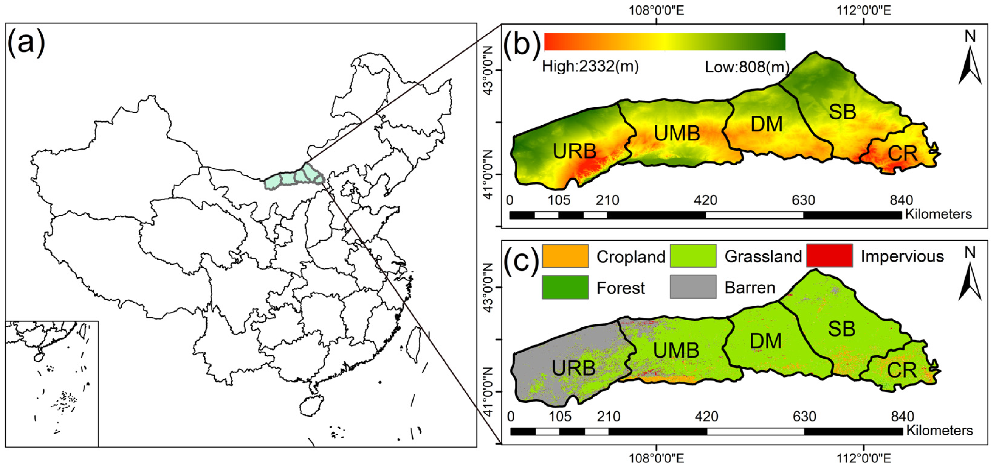
2.1. Study Area

The NFYM is in the northern region of Inner Mongolia, bordering Mongolia, which represents a transitional zone from the Yin Mountain range to the Mongolian Plateau and is characterized by an intricate mix of agricultural and pastoral landscapes. The NFYM encompasses five leagues: Urad Rear Banner (URB), Urad Middle Banner (UMB), Darhan Muminggan United Banner (DM), Siziwang Banner (SB), and Chahar Right Rear Banner (CR) (Figure 1). Predominantly subjected to arid and semi-arid climates, the NFYM experiences an average annual precipitation ranging from 100 to 400 mm. Additionally, the region has an annual average wind speed ranging from 2 to 6 m/s. The majority of the NFYM consists of severely degraded grasslands with a simple ecosystem structure and a weak ability for self-regulation and recovery. Furthermore, the NFYM is highly vulnerable to human interference and natural disasters, possesses poor water resources, and boasts an extremely fragile ecological environment. Moreover, it houses a substantial proportion of wind-eroded sandy land which serves as a primary source of sandstorms, posing a grave threat to the ecological security of North China.

2.2. Data Sources and Processing

In the NFYM, the contribution of Ei to E is negligible and can therefore be discounted (Figure A1). Due to the minimal proportion that Ei represents in the total E, this study quantitatively assessed the impacts of vegetation greening and climate change on the variations in E, Et, and Eb across the NFYM from 2000 to 2020.

The GLDAS_NOAH025_M product is a global high-resolution multi-parameter remote sensing land surface dataset generated by the Global Land Data Assimilation System (GLDAS) of the National Aeronautics and Space Administration (NASA) based on the NOAH land surface model (GES DISC Dataset: GLDAS Noah Land Surface Model L4 monthly 0.25 × 0.25 degree V2.1 (GLDAS_NOAH025_M 2.1) (https://uat.gesdisc.eosdis.nasa.gov/datasets/GLDAS_NOAH025_3H_EP_2.1, accessed on 1 January 2023). This product provides sub-daily and monthly data from January 2000 to near real time at a spatial resolution of 0.25° for various land surface parameters including E, Et, Eb, downward longwave radiation, downward shortwave radiation, air pressure, specific humidity, Pre, Temp, and WS. The data are available in formats such as GRIB and GeoTIFF. By assimilating satellite-based observations and ground-based measurements, this dataset can be widely applied for research in areas including large-scale climate change analysis, hydrological cycle modeling, and agricultural management [39,40,41]. RH was estimated using Equation (1) [42]:

$$\mathrm{R}\mathrm{H}=0.263\mathrm{p}\mathrm{q}{\left[{\mathrm{e}}^{\left(\frac{17.67\left(\mathrm{T}-{\mathrm{T}}_0\right)}{\mathrm{T}-29.65}\right)}\right]}^{-1},$$

(1)

where p represents pressure (Pa), q denotes specific humidity (dimensionless), T signifies temperature (K), and T₀ stands for the reference temperature (usually 273.16 K).

Rad was calculated according to Equation (2):

$$\mathrm{R}\mathrm{a}\mathrm{d}=\mathrm{L}\mathrm{R}\mathrm{a}\mathrm{d}+\mathrm{S}\mathrm{R}\mathrm{a}\mathrm{d},$$

(2)

where LRad represents downward longwave radiation, SRad denotes downward shortwave radiation, and Rad stands for the total radiation.

The Global Land Surface Satellite (GLASS) LAI product is a long-term (1982–2020) global Leaf Area Index (LAI) dataset generated from surface reflectance data acquired by the Moderate Resolution Imaging Spectroradiometer (MODIS) sensor onboard NASA’s Earth Observing System (EOS) satellites (Index of /LAI/MODIS/0.25 D (http://www.glass.umd.edu/LAI/, accessed on 11 January 2023)). With a spatial resolution of 0.05° and temporal resolution of 8 days, the GLASS LAI data are derived using optimized vegetation index fitting models and quality controlled using multi-source references. Available in GeoTIFF format, the GLASS LAI product enables continuous global vegetation growth monitoring and terrestrial ecosystem research. Owing to its high quality, long-term continuity, and free accessibility, the GLASS LAI dataset has been widely utilized in global change studies [43,44,45]. Before data processing, for the purpose of validating the accuracy and usability of the GLDAS_NOAH025_M data product, we conducted a comparison between GLDAS E, Et, and Eb and their counterparts in GLEAM (Global Land Evaporation Amsterdam Model) (Figure A2). In particular, the means and rate of change for two distinct sets of data sources were computed and compared. Simultaneously, the Root Mean Square Error (RMSE) was calculated to elucidate the reliability of the data. The results indicate that the spatial distribution patterns of the means and rate of change for E, Et, and Eb in both data sets exhibit similarity. Moreover, the RMSE values, particularly at the spatial scale of the NFYM, were relatively small, with only slight increases observed in a minimal number of regions. Hence, the data product from GLDAS_NOAH025_M can be employed to investigate the spatiotemporal patterns of regional evapotranspiration and its components. Ensuring consistency in spatial resolution across all data domains, resampling of the aforementioned data at a resolution of 1000 m was conducted using bilinear interpolation in ArcGIS 10.8. This method involved estimating the value of a target point by considering the numerical values of its four adjacent points and utilizing linear relationships. This approach allowed for accurate estimation of target point values with favorable precision, without introducing excessive computational complexity.

Furthermore, the Advanced Spaceborne Thermal Emission and Reflection Radiometer Global Digital Elevation Model (ASTER GDEM), collaboratively produced by NASA and the Japan Aerospace Exploration Agency (JAXA), constitutes a global digital elevation model with a spatial resolution of 30 m. Accessible through the platform of Geospatial Cloud (https://www.gscloud.cn, accessed on 24 November 2022), this dataset is derived from satellite remote sensing data and furnishes precise elevation measurements for diverse geographical locations on Earth’s surface (Figure 1b). The China Land Cover Dataset (CLCD), curated by Professors Jie Yang and Xin Huang from Wuhan University, encompasses comprehensive data on diverse land categories within the geographical extent of China (Figure 1c). By amalgamating high-resolution remote sensing imagery and ground-level observations, this dataset contributes pivotal information to fields encompassing environmental investigation, agricultural management, water resource planning, and ecological conservation [46].

2.3. Methods

2.3.1. Theil–Sen Estimate

The Theil–Sen estimator is a robust non-parametric method utilized for the estimation of temporal trends within time series data. This method demonstrates insensitivity to measurement errors and aberrant observations, rendering it particularly applicable to the analysis of trends within extensive time series datasets [47,48,49,50]. Computation of the Theil–Sen estimator is achieved through Equation (3):

$$\mathrm{Slope}=\mathrm{Median}\left(\frac{{\mathrm{X}}_{\mathrm{j}}-{\mathrm{X}}_{\mathrm{i}}}{\mathrm{j}-\mathrm{i}}\right), \mathrm{Ɐ}\mathrm{i}<\mathrm{j},$$

(3)

where Slope represents the median of the estimated slopes when i ≠ j; and xi and xj denote the values of variable x in the ith and jth years (where i and j are numerical values representing years). Slope > 0 indicates an increasing trend of the variable within the given time series, and vice versa. The Theil–Sen estimator was employed on the obtained time series by mean values extracted from raster data.

2.3.2. Mann–Kendall Test

The Mann–Kendall (M-K) trend test is widely employed for trend analysis in non-normally distributed time series data [47,48,50]. The null hypothesis (H0) posits the absence of a significant increasing or decreasing trend within the time series, while the alternative hypothesis suggests a significant trend change within the time series. Assuming the time series of the variable is represented as X = (X1, X2, …, Xn), where n is the number of sample observations, the calculation formulas for the test statistic S are provided by Equations (4) and (5):

$$\mathrm{S}={\sum }_{\mathrm{i}=1}^{\mathrm{n}-1}{\sum }_{\mathrm{i}=\mathrm{i}+1}^{\mathrm{n}}\mathrm{sgn}\left({\mathrm{X}}_{\mathrm{j}}-{\mathrm{X}}_{\mathrm{i}}\right),$$

(4)

$$\mathrm{Sgn}\left({\mathrm{X}}_{\mathrm{j}}-{\mathrm{X}}_{\mathrm{i}}\right)=\left\{\begin{array}{c}+1, {\mathrm{X}}_{\mathrm{j}}-{\mathrm{X}}_{\mathrm{i}}>0\\ 0, {\mathrm{X}}_{\mathrm{j}}-{\mathrm{X}}_{\mathrm{i}}=0\\ -1, {\mathrm{X}}_{\mathrm{j}}-{\mathrm{X}}_{\mathrm{i}}<0\end{array}\right.,$$

(5)

When n ≥ 8, the test statistic S approximately follows a normal distribution with a mean E(S) = 0. The formula for calculating the variance Var(S) is provided by Equation (6):

$$\mathrm{Var}\left(\mathrm{S}\right)=\frac{\mathrm{n}\left(\mathrm{n}-1\right)\left(2\mathrm{n}+5\right)-\sum _{\mathrm{i}=1}^{\mathrm{n}}{\mathrm{t}}_{\mathrm{i}}(\mathrm{i}-1\left)\right(2\mathrm{i}+5)}{18},$$

(6)

where n represents the number of groups with equal data, and t_i denotes the number of members in the ith group of equal data. Further derivation leads to the standardized statistic Z, as given by Equation (7):

$$\mathrm{Z}=\left\{\begin{array}{c}\frac{\mathrm{S} - 1}{\sqrt{\mathrm{Var}\left(\mathrm{S}\right)}}, \mathrm{S}>0\\ 0, \mathrm{S}=0\\ \frac{\mathrm{S} + 1}{\sqrt{\mathrm{Var}\left(\mathrm{S}\right)}}, \mathrm{S}<0\end{array}\right.,$$

(7)

For a given significance level α, if $\mathrm{Z}\ge {\mathrm{Z}}_{1-\frac{\alpha }{2}}$, the null hypothesis is rejected, indicating that the sequence exhibits a significant trend at the confidence level α. Conversely, if this condition is not met, the null hypothesis is accepted, implying that the trend in the sequence is not significant. A positive Z value suggests the presence of an upward trend in the data sequence, while a negative Z value indicates a downward trend. This process allows for the determination of whether the observed trend is statistically significant based on the predefined confidence level α. The Mann–Kendall test was computed on the acquired time series by mean values extracted from raster data, encompassing the calculation of the standardized statistic Z and the detection of breakpoints.

2.3.3. Partial Correlation

Partial correlation (PC) is an analytical method used to assess the linear relationship between two variables while controlling for the influence of other variables. In comparison to simple correlation, partial correlation considers potential effects among multiple variables, while applying specific techniques to control for other variables. This method specifically examines the net correlation relationship between two variables. Taking the second-order partial correlation coefficient as an example, let the dependent variable be denoted as y, with independent variables x1 and x2. When examining the net correlation between variables x1 and y, while accounting for the linear impact of x2, the first-order partial correlation coefficient between x1 and y can be calculated using Equation (8):

$${\mathrm{r}}_{\mathrm{y}1,2}=\frac{{\mathrm{r}}_{\mathrm{y}1}-{\mathrm{r}}_{\mathrm{y}2}{\mathrm{r}}_{12}}{\sqrt{(1-{\mathrm{r}}_{\mathrm{y}2}^2\left)\right(1-{\mathrm{r}}_{12}^2)}},$$

(8)

where ${\mathrm{r}}_{\mathrm{y}1,2}$ represents the net partial correlation coefficient (PCC) between x1 and y after eliminating the linear influence of x2 on y, and ry1, ry2, and r12 represent the correlation coefficients between y and x1, y and x2, and x1 and x2, respectively. The magnitude of the partial correlation coefficient serves as an indicator of the strength of the linear association between variables. A larger absolute value signifies a stronger linear correlation, whereas a smaller value suggests a weaker correlation. In this study, partial correlation coefficients were calculated for each driving factor concerning E, Et, and Eb. The computation of spatial scale partial correlation relied on each pixel of the raster image. Calculations were performed for each pixel, where each pixel contained yearly data from 2000 to 2020 for various variables.

2.3.4. Multiple Regression and Contribution Analysis

Multiple Regression Analysis (MRA) involves considering one variable as the dependent variable and the other variables as independent variables among the correlated variables. It establishes mathematical models or quantitative relationships, either linear or nonlinear, among multiple variables and evaluates the explanatory power of different independent variables on the dependent variable. We present Equation (9) as follows:

$$\mathrm{Y}={\mathsf{\beta }}_0+{\mathsf{\beta }}_1{\mathrm{X}}_1+{\mathsf{\beta }}_2{\mathrm{X}}_2+\cdots +{\mathsf{\beta }}_{\mathrm{k}}{\mathrm{X}}_{\mathrm{k}}+\mathsf{\epsilon },$$

(9)

This is referred to as the population regression model, where ${\mathsf{\beta }}_0,{\mathsf{\beta }}_1,{\mathsf{\beta }}_2,\cdots ,{\mathsf{\beta }}_{\mathrm{k}}$ are known as regression parameters. Taking the expectation on both sides of Equation (9) yields the population regression Equation (10):

$$\mathrm{E}\left(\mathrm{Y}\right|{\mathrm{X}}_1,{\mathrm{X}}_2,\cdots ,{\mathrm{X}}_{\mathrm{k}},)={\mathsf{\beta }}_0+{\mathsf{\beta }}_1{\mathrm{X}}_1+{\mathsf{\beta }}_2{\mathrm{X}}_2+\cdots +{\mathsf{\beta }}_{\mathrm{k}}{\mathrm{X}}_{\mathrm{k}},$$

(10)

where $\mathrm{E}\left(\mathrm{Y}\right|{\mathrm{X}}_1,{\mathrm{X}}_2,\cdots ,{\mathrm{X}}_{\mathrm{k}},)$ represents the conditional mean of the observed value Y given the independent variables X_i. We estimate the corresponding population parameters based on the sample observations as ${\mathsf{\beta }}_0,{\mathsf{\beta }}_1,{\mathsf{\beta }}_2,\cdots ,{\mathsf{\beta }}_{\mathrm{k}}$, resulting in the sample regression equation as shown in Equation (11):

$$\widehat{\mathrm{Y}}={\widehat{\mathsf{\beta }}}_0+{\widehat{\mathsf{\beta }}}_1{\mathrm{X}}_1+{\widehat{\mathsf{\beta }}}_2{\mathrm{X}}_2+\cdots +{\widehat{\mathsf{\beta }}}_{\mathrm{k}}{\mathrm{X}}_{\mathrm{k}},$$

(11)

where $\widehat{\mathrm{Y}}$ is the estimate of $\mathrm{E}(\mathrm{Y}{\mathrm{X}}_1,{\mathrm{X}}_2,\cdots ,{\mathrm{X}}_{\mathrm{k}},)$. The parameters are estimated using the method of least squares, assuming Equation (12):

$$\mathrm{Q}=\sum {({\mathrm{Y}}_{\mathrm{i}}-{\widehat{\mathrm{Y}}}_{\mathrm{i}})}^2=\sum ({\mathrm{Y}}_{\mathrm{i}}-{\widehat{\mathsf{\beta }}}_0-{\widehat{\mathsf{\beta }}}_1{\mathrm{X}}_1-{\widehat{\mathsf{\beta }}}_2{\mathrm{X}}_2-\dots -{\widehat{\mathsf{\beta }}}_{\mathrm{k}}{\mathrm{X}}_{\mathrm{k}})=\min ,$$

(12)

Partial derivatives of Q with respect to ${\mathsf{\beta }}_0,{\mathsf{\beta }}_1,{\mathsf{\beta }}_2,\cdots ,{\mathsf{\beta }}_{\mathrm{k}}$ are calculated as shown in Equation (13):

$$\left\{\begin{array}{c}\frac{\partial \mathrm{Q}}{\partial {\widehat{\mathsf{\beta }}}_0}=\sum \left({\mathrm{Y}}_{\mathrm{i}}-{\widehat{\mathsf{\beta }}}_0-{\widehat{\mathsf{\beta }}}_1{\mathrm{X}}_1-{\widehat{\mathsf{\beta }}}_2{\mathrm{X}}_2-\dots -{\widehat{\mathsf{\beta }}}_{\mathrm{k}}{\mathrm{X}}_{\mathrm{k}}\right)\left(-1\right)=0\\ \frac{\partial \mathrm{Q}}{\partial {\widehat{\mathsf{\beta }}}_1}=\sum \left({\mathrm{Y}}_{\mathrm{i}}-{\widehat{\mathsf{\beta }}}_1-{\widehat{\mathsf{\beta }}}_0{\mathrm{X}}_0-{\widehat{\mathsf{\beta }}}_2{\mathrm{X}}_2-\dots -{\widehat{\mathsf{\beta }}}_{\mathrm{k}}{\mathrm{X}}_{\mathrm{k}}\right)\left(-1\right)=0\\ \text{⋮}\\ \frac{\partial \mathrm{Q}}{\partial {\widehat{\mathsf{\beta }}}_{k-1}}=\sum \left({\mathrm{Y}}_{\mathrm{i}}-{\widehat{\mathsf{\beta }}}_k-{\widehat{\mathsf{\beta }}}_0{\mathrm{X}}_0-{\widehat{\mathsf{\beta }}}_1{\mathrm{X}}_1-\dots -{\widehat{\mathsf{\beta }}}_{\mathrm{k}-1}{\mathrm{X}}_{\mathrm{k}-1}\right)\left(-1\right)=0\end{array}\right.,$$

(13)

The estimated values of the parameters ${\widehat{\mathsf{\beta }}}_0,{\widehat{\mathsf{\beta }}}_1,{\widehat{\mathsf{\beta }}}_2,\cdots ,{\widehat{\mathsf{\beta }}}_{\mathrm{k}}$ are obtained by solving the above system of equations. In this study, standardization was applied to the variables to address the issue of differing scales. Subsequently, MRA was employed to estimate the values of the coefficients ${\widehat{\mathsf{\beta }}}_0,{\widehat{\mathsf{\beta }}}_1,{\widehat{\mathsf{\beta }}}_2,\cdots ,{\widehat{\mathsf{\beta }}}_{\mathrm{k}}$ for each driving factor, representing their respective contributions to E and its components [51,52,53,54].

According to the contribution degrees obtained by MRA, using the method of [4], we identified the spatial dominant factors. First, the E change rate within the study period was evaluated for each pixel. Pixels exhibiting a positive E change rate were considered to be primarily driven by the predictor variable corresponding to the maximum regression coefficient derived from multivariate analysis. Conversely, for pixels displaying a negative E change rate, the dominant factor was identified as the variable associated with the minimum regression coefficient. For instance, in a region where E showed an increasing trend, Pre had the maximum coefficient among all drivers calculated by MRA. Hence, Pre was determined as the dominant factor governing the E change in this region. Based on this approach, by comparing the E temporal derivative to zero, the predominant control at each pixel could be delineated according to the most positively or negatively correlated determinant that emerged from the multivariate regression modeling. This method takes advantage of spatial heterogeneity in the inherent relationships between E and various potential forcing factors. Therefore, the locally derived regression coefficients facilitate the attribution of the variable with the greatest explanatory power on E change as the governing control for each responsive pixel. The calculations for MRA were also conducted on a pixel-wise basis. We iteratively extracted the corresponding pixels for each factor, obtaining time series data for each variable. Subsequently, the aforementioned calculations were applied to each pixel, with the process automatically progressing to the next pixel. This sequential approach enabled the realization of spatial MRA.

2.3.5. Path Analytic Method

PC and MRA can only reflect the direct impacts of various environmental factors on E and its components, but they cannot elucidate the indirect effects of vegetation and climatic factors on E. Therefore, to accurately quantify the mechanistic roles of climate change and vegetation greening on E, we employed path analysis (PA) to dissect the direct and indirect effects of different climatic variables and LAI on the variations in E and its components. PA was first introduced by geneticist Sewell Wright in 1921 as a mathematical and statistical technique. Today, the application of this method is prevalent in the field of biology [55,56,57]. The advantage of this method is its capability to separate correlation coefficients into direct and indirect effects in situations where there is a high number of independent variables and intricate relationships among them. For instance, some relationships among independent variables may be correlational, while others may be causal. Additionally, this method is useful when certain independent variables indirectly impact the dependent variable through other independent variables. Path analysis enables the quantification of both direct and indirect effects of individual driving factors on variable E and its constituent components. In this study, we utilized standardized meteorological data and LAI data as input and intermediate variables, while E, Et, and Eb were considered as the output variables [58]. All path analyses were conducted using the package lavaan in R 4.2.2 [59,60,61]. Specifically, the normalized yearly means of each variable were input into the pre-constructed path model, facilitating path analysis.

3. Results

3.1. Spatiotemporal Variations in E and its Components

3.1.1. Temporal Patterns

Based on the annual gridded data of E, Et, and Eb in the NFYM from 2000 to 2020, we extracted the average values of the entire grid for each year to represent the annual values of evapotranspiration, transpiration, and soil evaporation. Subsequently, an analysis of the interannual variation trends of evapotranspiration and its components was conducted. Temporally, the E exhibited a significant (p < 0.01) increasing trend with a rate of 2.47 mm/a in the study area from 2000 to 2020 (Figure 2a). A detected change point in 2012 marked a transition from prior fluctuating variations to a stable growth pattern (Figure 2b). Similarly, Eb displayed a significant increasing trend (p < 0.01) at a rate of 1.06 mm/a (Figure 2a), showing a similar trend to E, and also revealing an abrupt change point in 2012 (Figure 2c). The trend in Et showed a significant increase (p < 0.01) at a rate of 1.30 mm/a, punctuated by six detected change points during this period. The last change point also occurred in 2012, followed by a period of stable growth (Figure 2d). As shown in Figure 2, the contribution of Eb to the change in E exceeded that of Et. The beneficial impacts of vegetation restoration efforts became increasingly discernible after the year 2012.

3.1.2. Spatial Patterns

Spatially, the regions with high average E values over multiple years were concentrated in the southeastern part of the NFYM, encompassing mainly the southeastern portion of the UMB, the southern part of the DM, the southern part of the SB, and the entire CR area, reaching a maximum E value of 322.28 mm. The regions with low E values were primarily found across the entire URB area, with a minimum E value of 68.59 mm. Generally, there is a decreasing trend in E from east to west (Figure 3a). The Et ranged between 0.87 mm and 236.55 mm, increasing from southeast to northwest. High Et values were observed in the southern parts of the DM and the SB, as well as the entire CR (Figure 3b), while regions with low values were widely distributed in most areas of the NFYM. The range of Eb values spanned from 66.11 mm to 205.32 mm, with high values predominantly distributed in the central part of the NFYM, including the central portion of UMB, the northwestern part of the DM, and the northwestern and northeastern parts of the SB (Figure 3c). The low Eb values were observed in the entire URB, the southern part of the SB, and the southern part of the CR, among other areas.

We analyzed the trends and significance of changes in E, Et, and Eb during 2000–2020 (Figure 4). The change rates of E were positive, with high values concentrated in the central and southwestern parts of the UMB, the southwestern part of the DM, the northeastern part of the SB, and the border areas with the CR. These areas exhibited a significant increasing trend (23.42%), with the highest change rate of 4.76 mm/a. The change rate for Et was predominantly positive, with a few negative values observed in the southern part of the DM and the northwestern part of the SB, while these changes were not significant. Significant growth in Et was observed over nearly the entire URB, the central-western part of the UMB, and the southwestern part of the SB. Areas exhibiting a significant increase accounted for 53.68% of the total study region. The highest growth rate is found in the southeastern part of the SB and the southwestern part of the CR, where the rate of change reaches a maximum of 5.59 mm/a. Regions exhibiting significant increases in Eb were distributed sporadically across the NFYM, comprising 8.86% of the total area. The maximum Eb increase rate attained was 3.88 mm/a within these responsive zones. However, a decreasing trend was observed in the southern parts of the SB and the CR.

3.2. Changes in LAI and Climatic Variables

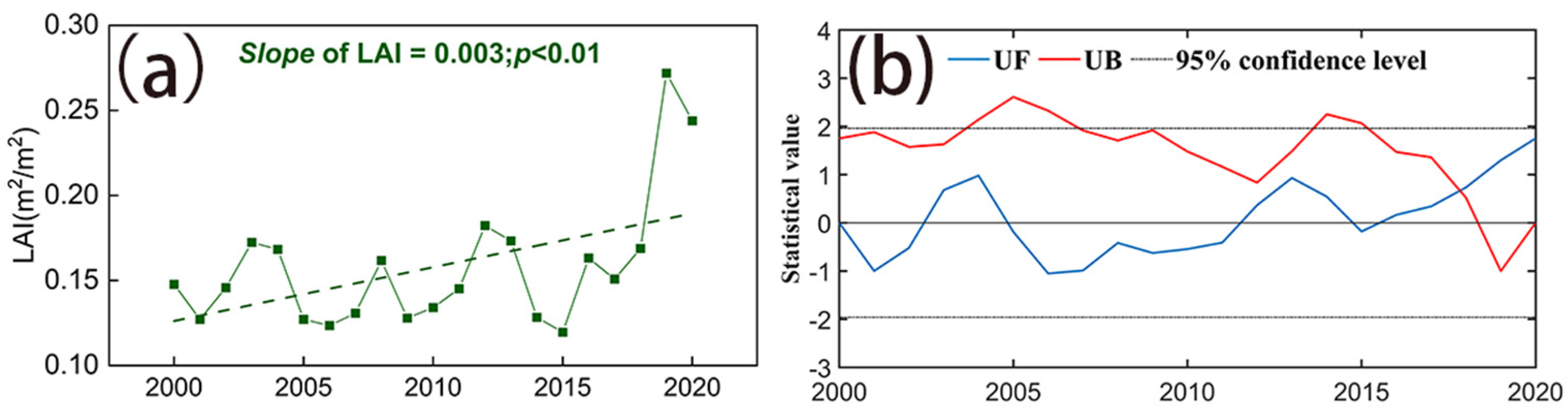
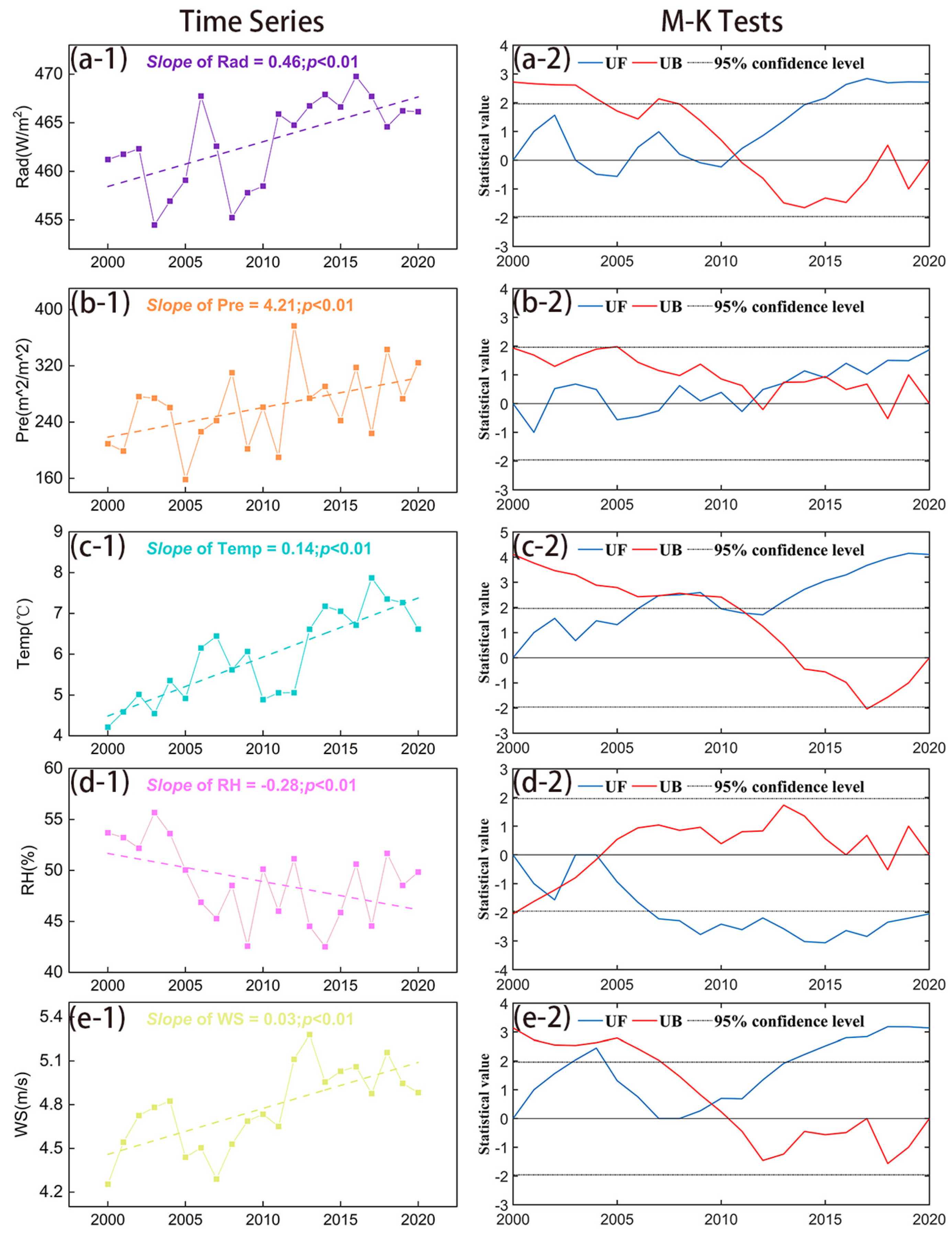
3.2.1. Temporal Variability

Based on the remote sensing meteorological and vegetation data for the NFYM from 2000 to 2020, the average values of the entire gridded dataset were extracted for each year to represent the annual values of meteorological elements and vegetation data. Subsequently, we analyzed the interannual variation trends. Before quantifying the impacts of vegetation greening and climate change on E, Et, and Eb, we initially examined the changes in vegetation LAI and climate factors. For the temporal scale, LAI exhibited an overall increase at a rate of 0.003 m²/m²/a and displayed gradual fluctuations during the period of 2000–2018 (Figure 5a), followed by a significant growth surge and a prominent increase in 2018 (Figure 5b). The annual variations in climate factors (Rad, Pre, Temp, RH, and WS) within the NFYM from 2000 to 2020 are presented in Figure 6. The average annual Rad showed a significant upward trend with an increase of 0.46 W/m²/a, featuring a distinct upward mutation in 2011. Pre exhibited a significant increase with a rate of 4.21 mm/a and underwent an upward mutation in 2012. The change rate of Temp was 0.14 °C/a, showing multiple detected upward mutation points, with the last one occurring in 2013. RH demonstrated a downward trend at a rate of 0.28%/a, characterized by the identification of three decreasing mutation points. WS increased at a rate of 0.03 m/s/a, with an upward mutation point detected in 2009. Overall, the study period exhibited intricate and diverse variations in both vegetation and meteorological factors.

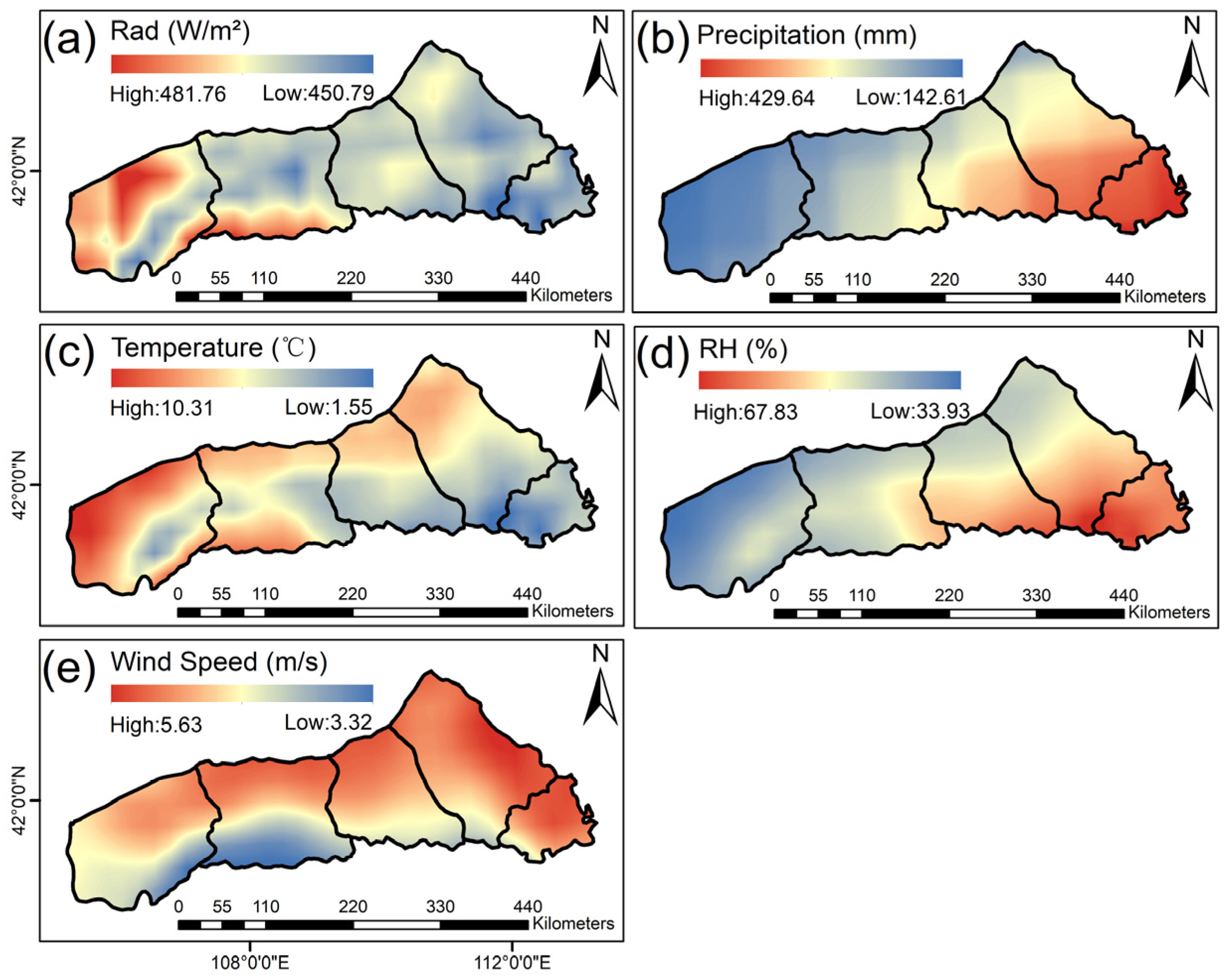
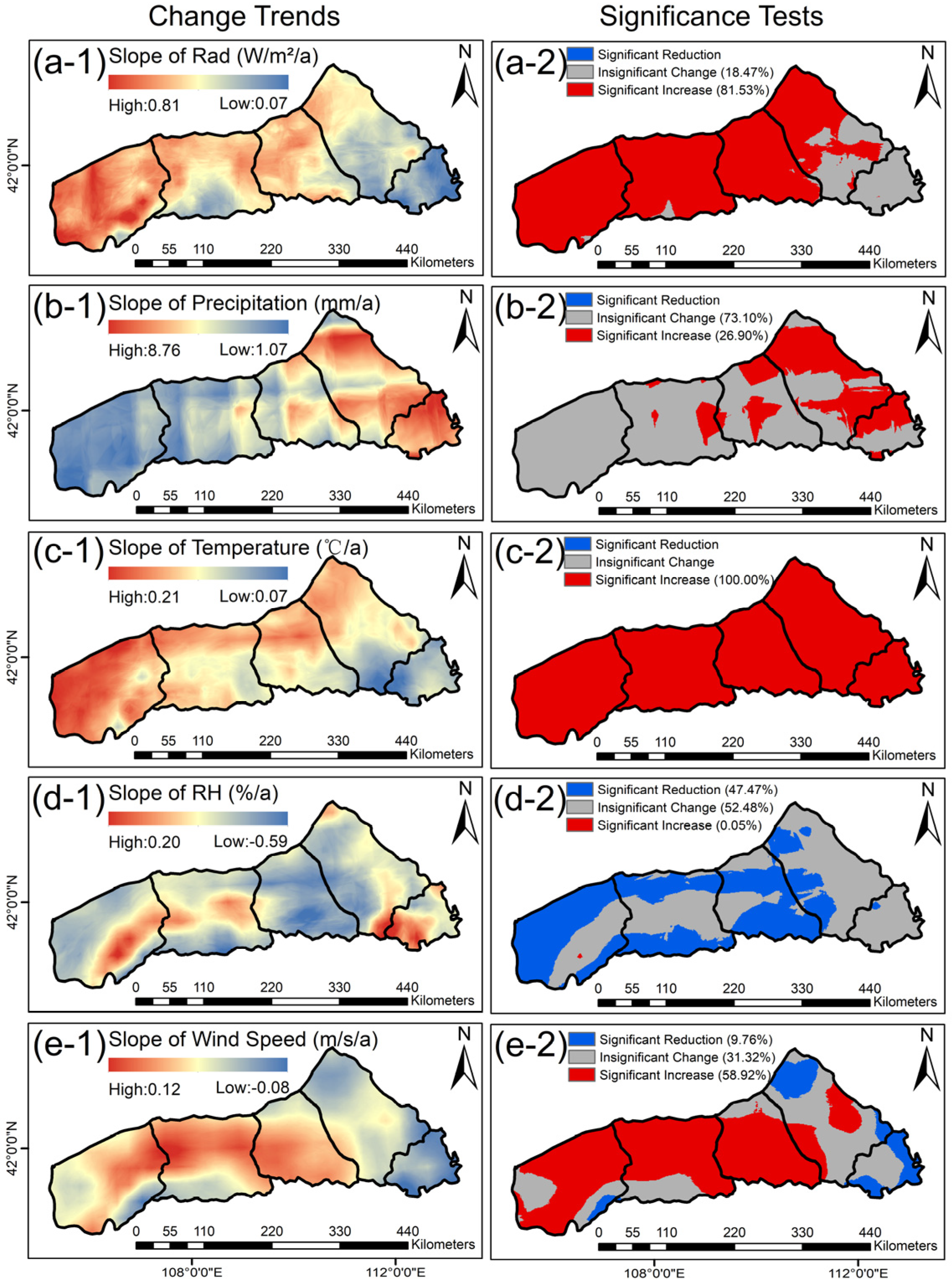
3.2.2. Spatial Variability

In terms of spatial distribution, the multi-year average LAI exhibited relatively low levels, with high values concentrated in the southern part of the NFYM due to the influence of the Yellow River Basin’s ecological restoration policies. Most other regions had comparatively lower vegetation coverage (Figure 7a). Significant increases in LAI were observed in the southern and central parts of the UMB, the central and southern parts of the SB, and the southwestern part of the CR, accounting for 13.78% of the NFYM, which could be attributed to the NFYM’s active implementation of ecological projects’ “Main battlefield”. Conversely, regions with significantly decreased LAI were scattered in the URB, accounting for 5.41% of the total area, possibly linked to factors such as grassland degradation, overgrazing, and abandonment (Figure 7c).

The spatial distribution characteristics of annual average meteorological variables are illustrated in Figure 8. Furthermore, Figure 9 displays the spatial distribution of the change rate in meteorological factors along with the results of the significance tests. For Rad distribution, the highest values were found in the northwest of the URB and the southern part of the UMB, reaching a maximum of 481.76 W/m², while the lowest value was 450.79 W/m² (Figure 8a). The change rate ranged between 0.07 W/m²/a and 0.81 W/m²/a, exhibiting an overall decreasing trend from northwest to southeast (Figure 9(a1)). Except for the southeast of SB and the entire CR, significant increases were evident in other regions (Figure 9(a-2)). Pre exhibited substantial spatial variability, decreasing from southeast to northwest, with the highest values in the southeast of the NFYM reaching up to 429.64 mm, while the lowest values in the northwest part being only 142.61 mm (Figure 8b). High Pre areas also witnessed significantly increased change rates, with the highest reaching 8.76 mm/a, gradually decreasing to 1.07 mm/a towards the west (Figure 9(b-1)). The spatial distribution of Temp was closely related to elevation (Figure 9(c-1)), showing a significant increasing trend across the entire study area (Figure 9(c-2)). Average Temp (1.55 °C) and change rates (0.07 °C/a) were lower in the high-altitude mountain ridges, whereas lower elevations exhibited higher temperatures, reaching up to 10.31 °C, with the highest change rate at 0.21°C/a (Figure 9(c-1)). The multi-year average RH decreased from southeast to northwest, resembling the spatial pattern of Pre, ranging between 33.93% and 67.83%, indicating significant differences in humidity between the eastern and western regions (Figure 8d). RH significantly decreased at the northern and southern boundaries of the NFYM (Figure 9(d-2)), with the fastest rate at 0.59%/a. In the high-altitude regions of the URB, UMB, and CR, RH exhibited a slow-increasing trend, peaking at approximately 0.20%/a (Figure 9(d-1)). WS displayed an increasing trend from the southwest to the northeast, ranging between 3.32 m/s and 5.63 m/s (Figure 8e). The northeast part of the URB, the northern part of the UMB, and the southern part of the DM experienced a significant increase at a rate of approximately 0.12 m/s/a, while the northeast part of the SB and the southern boundary of the CR witnessed a notable decrease at a rate of around 0.08 m/s/a (Figure 9(e-1))). In conclusion, despite gradual vegetation recovery due to ecological restoration measures, the NFYM’s vegetation coverage remained relatively low, and effective measures against grassland degradation are still needed. The complex and diverse meteorological environment in the NFYM results from its varied topography, wide lateral span, and spatially diverse meteorological conditions.

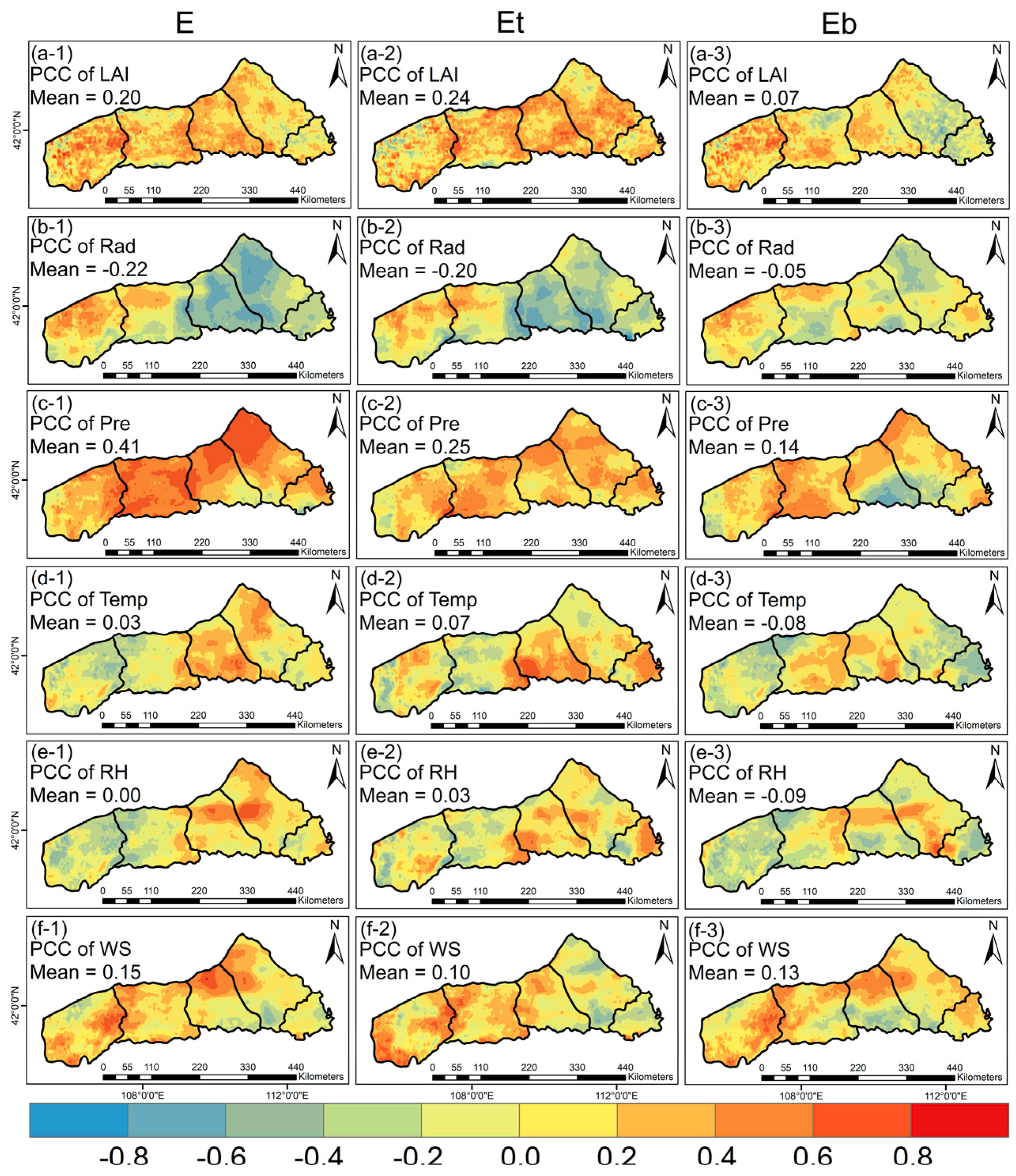
3.3. Changes in E, Et, and Eb Caused by Vegetation Greening and Climate Change

To assess the direct influences of driving factors on the variations in E, Et, and Eb within the NFYM from 2000 to 2020, we conducted partial correlation analyses between E, Et, and Eb and LAI and meteorological factors (Figure 10). Pre exhibited the strongest correlation with E, and the PCC of Pre was 0.41. The highest partial correlations were observed in the entire UMB, as well as in the northern parts of the DM and SB (Figure 10(a-3)). Rad displayed an average PCC of −0.22 with E, with positive correlations accounting for 72.17% of the area, mainly concentrated in the northwest of the NFYM, while the eastern part exhibited predominantly negative correlations (Figure 10(a-2)). The PCC between LAI and E was 0.20, with positive correlations covering 83.75% of the area, predominantly distributed as scattered points and clusters across the NFYM (Figure 10(a-1)). WS exhibited a moderate positive correlation with E, primarily concentrated in URB and UMB, as well as the boundary between the DM and SB, accounting for 71.67% of the area, with an average PCC of 0.15 (Figure 10(a-6)). The correlations of Temp and RH with E were relatively weak (Figure 10(a-4,a-5)). Strong correlations were observed between LAI and Pre with Et, with PCC values of 0.24 and 0.25, respectively. Positive correlations accounted for 85.80% and 91.04% of the area, respectively. LAI exhibited scattered positive correlations, while Pre exhibited a positive correlation in most regions except for the western part of the URB and the northwest part of the UMB (Figure 10(b-1,b-3)). Rad displayed an overall negative correlation with Et, with a PCC of −0.20. Negative correlations were prominent to the east of the UMB, accounting for 74.23% of the area, whereas positive correlations were evident to the west, indicating significant spatial differences (Figure 10(b-2)). WS exhibited a weak positive correlation with Et, covering approximately 63.72% of the area (Figure 10(b-6)). Temp and RH exhibited weak correlations with Et, with PCC values being less than 0.10 (Figure 10(b-4,b-5)). Comparatively, LAI and meteorological factors displayed lower correlations with Eb compared to E and Et. The highest PCC was observed between Pre and Eb, reaching 0.14, with positive correlations covering 75.64% of the area, predominantly concentrated in the western and northern parts of the NFYM (Figure 10(c-3)). WS exhibited the second-highest PCC with Eb, reaching 0.13, and displayed a similar spatial distribution pattern to Pre (Figure 10(c-6)). The PCC values of the remaining factors with Eb were all below 0.10. Similar to E and Et, Rad exhibited a negative correlation with Eb (PCC = −0.05), with negative correlations mainly concentrated in the northeast and south of the NFYM, covering 56.30% of the area. Temp and RH displayed negative correlations with Eb, with PCC values of −0.08 and −0.09, respectively (Figure 10(c-2,c-4,c-5)). Additionally, LAI exhibited a weak positive correlation with Eb, covering 62.04% of the area and being sporadically distributed to the west of the DM (Figure 10(c-1)).

The spatial patterns of contributions of LAI and climatic factors to the variations in E, Et, and Eb during the period of 2000–2020 are depicted in the spatial distribution presented in Figure 11. Among these factors, vegetation greening had the most pronounced impact on E, with LAI contributing an average of 0.49 mm/a. Positive contribution zones covered 83.75% of the total area, and areas with a contribution rate exceeding 0.8 mm/a were predominantly situated in the URB, constituting 19.15% of the NFYM (Figure 11(a-1)). Among the climatic factors, Pre yields the most significant contribution to E, augmenting it at a rate of 0.46 mm/a. A notable 92.44% of the study area demonstrated a positive contribution, particularly evident in the east of the URB, across the entire UMB, DM, SB, and CR northern zones (Figure 11(a-3)). The contribution of Rad to E exhibits spatial heterogeneity. It is segregated predominantly at the boundary of the central UMB, contributing positively to the east and negatively to the west. Negative contribution zones encompassed 72.17% of the region, leading to an average reduction rate of 0.36 mm/a (Figure 11(a-2)). WS contributed to E with an average rate of 0.17 mm/a, and positive contribution zones account for 71.67% of the total area. Notably, regions exceeding 0.8 mm/a were concentrated in the northern parts of the DM, as well as in the southern parts of the URB and UMB (Figure 11(a-6)). RH contributed negatively to E at a rate of −0.09 mm/a, with a balanced distribution of positive and negative contribution zones. The western URB and UMB predominantly exhibited negative contributions (49.55%), whereas the eastern Three-Flag Area mainly manifested positive contributions (Figure 11(a-5)). In contrast, Temp contributed at a slow rate of 0.08 mm/a, gradually increasing E. The contribution rate exhibited substantial spatial disparities, with regions exceeding 0.08 mm/a concentrated in the northwestern parts of the DM and SB, as well as in the northeastern URB, northwestern UMB, and certain areas of the SB and CR. Importantly, certain areas within these regions exhibited a more substantial reduction rate in E exceeding 0.8 mm/a, constituting 18.77% (Figure 11(a-4)). In terms of Et, climatic factors, particularly Temp, emerged as the primary drivers. Temp contributed to Et at a rate of 0.35 mm/a, with zones exceeding 0.8 mm/a primarily concentrated in the southeastern regions of the NFYM, accounting for 25.77%. Conversely, negative contribution zones were concentrated in the UMB, SB, and CR, constituting 44.24% of the total area (Figure 11(b-4)). In contrast, Rad exhibited a negative contribution of −0.30 mm/a to Et, with negative contribution zones covering 74.23% of the region. Positive contribution zones were limited mainly to the western parts of the UMB (Figure 11(b-2)). Pre also exerted a significant influence on Et, albeit less pronounced than the former, with a contribution rate of 0.19 mm/a. Positive contribution zones were widespread, accounting for 91.04% of the total area (Figure 11(b-3)). RH and WS exerted minor influences, contributing at rates of 0.04 mm/a and 0.03 mm/a, respectively (Figure 11(b-5,b-6)). Vegetation greening contributed 0.32 mm/a to Et, with positive contribution zones covering 85.80% of the total area, predominantly concentrated in the UMB and the adjacent eastern region (Figure 11(b-1)). In general, the individual impact of LAI, Rad, Pre, Temp, RH, and WS on Eb tends to be substantial, with contributions of 0.57 mm/a, −0.09 mm/a, 0.25 mm/a, 0.78 mm/a, −0.42 mm/a, and 0.25 mm/a, respectively. Positive contribution zones of LAI to Eb encompass 62.04% of the total area, with the highest positive contributions concentrated mainly in the western regions of the URB and UMB, while areas with high negative contributions were primarily concentrated in the southern parts of the CR and SB (Figure 11(c-1)). Negative contribution zones of Rad cover 56.30% of the total area, predominantly distributed in the southern parts of the UMB and the northern parts of the SB (Figure 11(c-2)). The contribution of Pre to Eb exhibited an increasing trend from southeast to northwest, transitioning from negative to positive contributions. Positive contribution zones covered 75.64% of the total area (Figure 11(c-3)). Temp demonstrated a bipolar phenomenon, with the central region of the NFYM showing higher positive contributions. Areas with a contribution rate exceeding 0.8 mm/a constitute 18.74% of the total area, while the flanking regions were dominated by areas with contribution rates exceeding −0.8 mm/a, accounting for 42.51% (Figure 11(c-4)). Positive contributions of RH to Eb presented a zonal distribution in the central region of the NFYM, accounting for 32.73%, predominantly influenced by negative contributions (Figure 11(c-5)). Positive contributions of WS encompassed 71.04% of the total area, with only a minor presence of negative contribution areas in the southeastern part of the NFYM (Figure 11(c-6)).

The spatial distribution of dominant factors influencing E, Et, and Eb over the NFYM is depicted in Figure 12. As shown in Figure 12a, Temp emerged as the dominant factor for E, covering 32.75% of the study area. It was primarily concentrated in the southern part of the DM and the northeastern portion of the SB. E driven by Pre dominated over 28.43% of the area, scattered across the UMB with concentrations in the southern SB and northern CR. Regions where LAI governs E changes were mainly situated in the URB, accounting for 25.01% of the study area. The remaining variations in E were primarily influenced by WS (7.84%), Rad (2.47%), and RH (3.49%). Figure 12b illustrates the dominant factor distribution for Et. Temp dominated in regions predominantly situated in the southern DM and southeastern CR, constituting the highest proportion at 33.83%. Et controlled by LAI covered 30.04% of the study area, primarily concentrated in the northern and eastern parts of the NFYM. Rad exerted dominance over 16.82% of the area, primarily located in the northwestern URB. Pre’s dominant areas were scattered and accounted for 12.02%. The influences of WS and RH were smaller, encompassing 4.46% and 2.44% of the area, respectively. From Figure 12c, it was evident that the primary dominant factors for Eb were LAI and Temp, covering 32.10% and 29.50% of the study area, respectively. Areas where WS dominates comprise 16.23% of the total, scattered across the DM, SB, and CR. Pre governed 14.34% of the area, while Rad (4.35%) and RH (3.47%) had relatively smaller controlling influences.

To further elucidate the direct and indirect effects of various driving factors on E, Et, and Eb of the NFYM, a path analysis was conducted. The results illustrated the direct dependencies of E, Et, and Eb on their respective variables (

Table 1. Path coefficients of factors. (“-” is used to indicate that there is no path relationship between the factors corresponding to different rows and columns within the constructed path model.)

Output Item	Factors	Direct Path Coefficients	The sum of Indirect Path Coefficients	Indirect Path Coefficients						Total Path Coefficients
				LAI	RAD	Temp	RH	WS	Pre
E	LAI	0.07	0.00	-	-	-	-	-	-	0.07
	Rad	−0.14	0.00	-	-	-	-	-	-	−0.14
	Temp	0.21	−0.19	-	−0.09	-	−0.10	-	-	0.03
	RH	0.13	−0.01	−0.01	-	-	-	-	-	0.13
	WS	0.20	0.13	0.01	-	0.11	0.00	-	-	0.33
	Pre	0.75	0.20	0.02	-	-	0.05	0.13	-	0.96
Et	LAI	0.22	0.00	-	-	-	-	-	-	0.22
	Rad	−0.08	0.00	-	-	-	-	-	-	−0.08
	Temp	0.17	−0.22	-	−0.05	-	−0.17	-	-	−0.05
	RH	0.22	−0.04	−0.04	-	-	-	-	-	0.18
	WS	0.36	0.14	0.05	-	0.09	0.07	-	-	0.50
	Pre	0.41	0.39	0.08	-	-	0.09	0.22	-	0.80
Eb	LAI	0.07	0.00	-	-	-	-	-	-	0.07
	Rad	−0.21	0.00	-	-	-	-	-	-	−0.21
	Temp	0.23	−0.29	-	−0.13	-	−0.16	-	-	−0.06
	RH	0.21	−0.01	−0.01	-	-	-	-	-	0.20
	WS	0.02	0.15	0.01	-	0.13	0.01	-	-	0.16
	Pre	0.84	0.12	0.02	-	-	0.08	0.01	-	0.96

). The final fitted Structural Equation Model (SEM) was presented in Figure 13. The model’s goodness-of-fit measures were satisfactory, with GFI (Goodness of Fit Index) exceeding 0.9, RMSEA (Root Mean Square Error of Approximation) below 0.10, CFI (Comparative Fit Index) exceeding 0.9, NFI (Normed Fit Index) exceeding 0.9, NNFI (Non-Normed Fit Index) exceeding 0.9, and a χ2/df ratio below 3. The constructed model accounted for 91% of E changes (R² = 0.92), 82% of Et changes (R² = 0.82), and 89% of Eb changes (R² = 0.89). Our findings suggested that LAI typically acted as an intermediate variable through which RH, WS, and Pre influenced E (RH→LAI→E, WS→LAI→E, Pre→LAI→E), with indirect path coefficients of −0.13, 0.01, and 0.02, respectively. LAI’s direct contribution to E exhibited a non-significant positive effect (0.07). Rad exerted a non-significant negative effect on E (−0.14), with an indirect path coefficient of −0.09 through Temp. Additionally, Temp indirectly influenced E through RH (Temp→RH→E), with a total effect of 0.01. The impact of WS on E encompassed the paths WS→LAI→E, WS→Temp→E, and WS→RH→E, yielding a total effect of 0.33. Pre, acting as an indirect variable, exhibited indirect effects on E by influencing other variables, through the paths Pre→LAI→E (p < 0.05), Pre→RH→E (p < 0.05), and Pre→WS→E, with indirect effects of 0.02, 0.05, and 0.13, respectively. The direct effect of Pre was 0.75, contributing to a total effect of 0.96 on E. For Et, LAI’s direct effect proved significant (0.22, p < 0.05). The combined effects of Rad and Temp on Eb were −0.080 and −0.05, respectively. PA and MRA results suggested varying effects of Temp on Et, possibly attributed to non-significant pathways. Pre, WS, and RH collectively exhibited total indirect effects on Et of 0.39, 0.36, and 0.22, resulting in overall effects of 0.79, 0.50, and 0.18, respectively. Regarding Eb, the most substantial total effect was attributed to Pre (0.96), followed by the negative effect of Rad (−0.21), and subsequently RH (0.20) and WS (0.16). Overall, the results of the path analysis and MRA were largely congruent, thereby providing mutual validation to the findings. It was evident that vegetation greening exerted a significant positive effect on Et, while exerting comparatively minor influences on E and Eb. In general, the changes in time and the intricacies in space of the climate continued to be important factors that affect E and its various elements.

4. Discussion

4.1. Spatiotemporal Variation in E, Et, and Eb

This spatiotemporal analysis provides new insights into the heterogeneous dynamics of E and its components across the NFYM from 2000 to 2020. The multi-year mean E ranged from 68.59 to 322.28 mm (Figure 3a), exhibiting an east-to-west decreasing trend likely linked to regional moisture and vegetation gradients. The E change rate significantly increased by 2.47 mm/a across most areas (Figure 2a), reflecting intensification congruent with climate and land surface changes. The consistent east-to-west descent in long-term E suggests the influence of regional gradients, potentially involving moisture availability, vegetation density, and other geo-environmental factors. Furthermore, the widespread positive change rates point to a prevailing escalation in E over the study period, indicative of climate and land surface shifts driving regional E intensification. Et displayed a southeast-to-northwest increasing gradient of 0.87–236.55 mm (Figure 3b), attributed to geographical vegetation variations. While Et mostly increased over time, localized decreasing trends were also detected. The Et change rate spanned −0.81 to 5.59 mm/a (Figure 4(b-1)), with a mean increase of 1.30 mm/a. Overall, the distinct Et spatial pattern appears linked to geographical variations in vegetation density and structure. Meanwhile, the differential temporal trends likely stem from localized land cover changes alongside background climatic warming and wetting influencing regional transpiration. However, additional factors related to soil moisture, vapor pressure deficit, and plant physiological shifts may also contribute to the complex spatiotemporal variability in Et. Lastly, Eb exhibited a northeast–southwest decreasing spatial pattern of 66.11–205.32 mm driven by climate and soil moisture influences (Figure 3c). The mean Eb change rate was low at 1.06 mm/a compared to Et (Figure 4(c-1)). Overall, the Eb geographical gradient arises from the effects of regional climate and soil moisture variability on evaporation from bare land surfaces. Meanwhile, the reduced spatiotemporal variability in Eb, compared to transpiration, likely stems from the dominant influence of atmospheric conditions on evaporation from bare soil. However, changes in bare ground cover fractions may also modulate Eb in some areas.

The aforementioned conclusions align with results reported in earlier investigations [37,38,62]. Typically, Et constitutes a significant portion of E [23,24]. However, as shown in Figure 2, it is evident that E is primarily composed of Eb, likely due to extensive grassland degradation and sparse vegetation cover. Geographically, the steep topography and marked elevation gradients promote rapid surface runoff, increasing horizontal water fluxes and bare soil evaporation. Aerodynamically, the north-facing slopes may obstruct southward air masses, enhancing updrafts and vertical moisture transport and further elevating Eb. Collectively, these geographic and atmospheric dynamics, coupled with limited transpiring vegetation, lead to the prevalence of Eb over Et across this vulnerable landscape. The detected spatial patterns and temporal shifts point to primary regulation by geographical gradients in vegetation and regional climate factors. However, the complex interactions between atmospheric conditions, soil moisture, plant physiology, and land cover change also appear to modulate the multi-faceted spatiotemporal variability in transpiration and bare soil evaporation. Further parsing of the relative contributions of these drivers is still needed through approaches integrating in situ data, process-based modeling, and remote sensing observations. Overall, the distinct spatial heterogeneity and escalating temporal trends in E revealed by this study underscore the impacts of recent environmental change across this ecologically vulnerable landscape. The findings pave the way for disentangling the complex environmental controls across the mountain region and developing adaptive water management strategies in the face of climate change and human activities. Consideration of both natural and anthropogenic drivers will be essential to elucidate the coupled vegetation–climate–hydrology system interactions governing E dynamics.

4.2. Responses of E, Et, and Eb to Vegetation Greening and Climate Change

The direct and indirect impacts of driving factors on E and its components were analyzed through MRA and PA, elucidating the mechanistic responses of E, Et, and Eb to vegetation greening and climate change. Research has indicated that vegetation greening has a clear positive impact on regional E processes. This is because changes in vegetation cover can regulate rainfall interception and alter surface roughness and albedo, thereby influencing the E process [63,64]. Our study reveals that vegetation greening has been the primary driving force behind the increase in E over the NFYM since 2000. The enhanced greening has contributed to an E growth rate of 0.49 mm/a, aligning with the aforementioned perspectives. LAI reflects the density and extent of vegetation coverage, directly determining the plant surface area available for transpiration. As LAI increases, the vegetated area expands, enlarging the total leaf surface for transpiration. This leads to a greater moisture surface area, with more water uptake from the soil to supply plant transpiration needs. LAI is also closely associated with photosynthesis, whereby vegetation absorbs and fixes CO₂ while concomitantly releasing water vapor to facilitate gas exchange. Higher LAI enables greater light capture for photosynthesis, releasing more moisture into the atmosphere through transpiration. Moreover, elevated LAI is typically accompanied by more dense stomata, expanding the transpiring surface and further promoting water loss. Among meteorological factors, Pre exhibits the largest contribution, increasing E at a rate of 0.46 mm/a (Figure 11(a-3)). Pre exerted highly significant direct effects on the increase in E, while also indirectly influencing E through impacts on LAI, RH, and WS. One possible explanation is that Pre and E are integral components of the water cycle. Changes in Pre directly influence the exchange of water vapor between the land surface and the atmosphere, subsequently affecting E. Moreover, substantial precipitation can indirectly impact E. As a vital water resource, precipitation significantly affects vegetation growth and soil moisture content. Adequate rainfall can satisfy plant water needs, promoting lush vegetation growth and resulting in higher LAI values, inducing greater transpiration potential. Additionally, precipitation alters environmental moisture content, thereby influencing air humidity. Meanwhile, rainfall events can prompt localized airflow disturbances, transiently impacting wind speed and indirectly affecting evaporation intensity. Rad contributes to a decrease in E at a rate of 0.36 mm/a (Figure 11(a-2)). This may be attributed to the effect of high radiation. Factors such as elevated temperature, increased water demand, water limitation, humidity influences, energy balance considerations, and wind speed effects under high radiation conditions could collectively suppress E variations. This is consistent with the intricate role of radiation in surface energy balance and its complex impact on temperature and water vapor evaporation. Notably, some previous studies on the correlation between E and climatic factors have indicated a relationship with temperature changes, which is not pronounced in our research. There are two potential explanations for this discrepancy: Firstly, prior work has shown that temperature changes themselves do not always provide a satisfactory indicator influencing E variations [65], as actual E is often constrained by water availability in arid and semi-arid regions [66]. Secondly, we posit that differences in topography and landforms may also lead to shifts in the temperature–evaporation association. The terrain characteristics in mountainous areas can affect localized airflow and humidity distributions, resulting in moist air retention and dampening the E response to temperature fluctuations.

Meteorological factors play a more significant role in influencing Et, particularly Temp, which increases Et at a rate of 0.35 mm/a. Notably, our MRA results indicated that Temp accelerated Et increase, while PA revealed an opposite effect (Temp directly promoted Et, but Temp’s highly significant positive contribution to Rad suppressed Et). Although ostensibly paradoxical, we posit that these findings are reconcilable, potentially stemming from methodological distinctions in evaluating direct versus indirect effects. Specifically, MRA emphasizes analyzing the direct temperature–E association, potentially overlooking intermediary variables. In this context, elevated temperatures can increase evaporation rates because warmer conditions enhance liquid water’s molecular kinetic energy, promoting vaporization. Conversely, path analysis stresses variable interrelationships, considering potential mechanisms for indirect temperature impacts on E. For instance, the Stefan–Boltzmann law states that higher surface temperatures induce greater terrestrial radiation emission to the atmosphere. Heightened radiation triggers stomatal closure by vegetation to reduce water loss, thereby constraining transpiration. Such indirect effects could yield the suppressive temperature influence on E evident in the path analysis. From a plant physiology perspective, Temp’s direct positive influence on Et can be contemplated. Elevated temperatures can accelerate plant biochemical reactions and metabolic processes, providing more energy and substrates to support transpiration. Warmer conditions promote enzyme activities, cell division, and cell elongation underlying growth, further elevating plant transpiration. Additionally, temperature regulation of stomata is an important mechanism enhancing transpiration. Stomata are minute pores on leaf surfaces facilitating gas exchange, including water vapor release and oxygen uptake. Rising temperatures can increase plant cell osmotic pressure, opening stomata to discharge water and carbon dioxide, resulting in greater internal water diffusion outward. Through stomatal control, plants concurrently regulate transpiration while mediating water and gas exchange to maintain intracellular/extracellular water balance and gas concentration equilibrium. Vegetation greening contributes 0.32 mm/a to Et, second only to Temperature, aligning with our understanding. Conversely, Rad reduces Et at a rate of 0.30 mm/a. This may involve a series of intricate physiological processes in plants. Under high temperatures, plants experience heat stress, leading to increased photosynthetic rates but slowed growth and stomatal closure. Simultaneously, high radiation might accelerate soil moisture depletion, restricting plant root water uptake and consequently impacting transpiration—a manifestation of plants’ external self-protection. Pre primarily enhances Et by promoting water supply to plants and improving the growth environment, contributing 0.19 mm/a.

Regarding Eb, LAI has the strongest promoting effect, leading to an increase in Eb at a rate of 0.57 mm/a. Rad, Pre, Temp, RH, and WS—five meteorological factors—exert independent impacts on Eb, with rates of −0.09 mm/a, 0.25 mm/a, 0.78 mm/a, −0.42 mm/a, and 0.25 mm/a, respectively (Figure 11c). Meteorological factors exhibit complex interplay governing Eb. Firstly, for Rad, heightened irradiance typically energizes water molecules, facilitating liquid-to-vapor phase shifts and enhancing evaporation. However, Rad suppressed Eb in southern UMB and northern SB, feasible under certain conditions; intense radiation at high Temp and low RH can prompt evaporation rates surpassing moisture supply, depleting surface water and suppressing vaporization. Secondly, Pre constitutes the primary water source, with greater rainfall providing more moisture for evaporation. Pre directly replenishes the land surface, furnishing ample water through soil wetting to sustain evaporation processes. Notably, the most pronounced inhibiting effect is associated with Temp, which contrasts with the conventional assumption that higher temperatures lead to greater Eb. In the arid region of the NFYM, this unexpected outcome may stem from soil moisture limitations; even with elevated temperatures, there might not be a sufficient water supply to support extensive surface water vapor evaporation. Regarding RH, our explanation for its negative contribution to Eb is that lower RH restricts the conversion of water from the liquid to the gas phase. Water molecules are less likely to transition to the gas phase under lower humidity, consequently reducing surface water vapor evaporation. High WS can enhance the diffusion of water vapor from the land surface into the atmosphere, thereby promoting surface water vapor evaporation.

4.3. Implications for Vegetation Restoration and Water Resources Management

The NFYM is located within the ecological security barrier of northern China and carries the crucial responsibility of acting as a barrier against sandstorms, wind erosion, and serving as a vital water source for the Beijing–Tianjin area. The research findings underscore the intricate interplay between the ecological condition of the NFYM and its cascading impacts on local economic development, poverty alleviation initiatives, as well as broader ecological security concerns at both regional and national scales. Thus, the NFYM holds a highly significant position in the context of ecological security strategy.

However, existing research attention towards the NFYM remains insufficient. Our study demonstrates that the increase in E, Et, and Eb in most areas of the NFYM is influenced by vegetation greening (Figure 12), closely related to local ecological restoration projects. Prior research indicates that vegetation greening can lead to increased water consumption, potentially heightening water scarcity risks [67]. Despite the current relatively low vegetation coverage in the NFYM, potential risks arising from vegetation restoration should still be continuously monitored. We propose that ongoing vegetation restoration efforts in the NFYM should continue, but with a comprehensive consideration of the potential negative impact of greening on water resources. Water-saving measures should be implemented, and the allocation of limited water resources should be rationalized. For instance, strategies such as thinning and understory vegetation control can be employed to generate more soil water, thereby replenishing groundwater and downstream water usage while increasing the available water supply for remaining vegetation [33,68]. Furthermore, while considering local environmental conditions, managers can select suitable vegetation species (those with lower water requirements and higher ecosystem benefits) to adjust the existing vegetation structure and composition. This optimization can balance ecological and hydrological benefits [69,70,71,72].

The insights gained from our investigation lend critical guidance for ongoing and future vegetation restoration initiatives within the NFYM in the context of climate change. The juxtaposition of increased vegetation cover and enhanced E underscores the necessity of judicious water resource management to mitigate potential water scarcity risks. As the ecological restoration projects within the NFYM gather momentum, our findings advocate for a holistic approach that harmonizes ecological and hydrological considerations. Implementing water-saving strategies and optimizing the selection of vegetation species, based on their water requirements and ecological benefits, represent crucial steps toward achieving a sustainable equilibrium between ecological enhancement and hydrological stability. In conclusion, this study’s implications extend beyond its immediate research scope, offering valuable insights into the broader domains of vegetation restoration and water resource management. As the NFYM assumes a strategic role in China’s ecological security strategy, our research serves as a beacon for informed decision making, highlighting the importance of a comprehensive approach that unites ecological restoration objectives with hydrological imperatives. The study’s findings hold immense potential to guide effective policy formulation and on-ground implementation strategies for sustainable vegetation restoration and water resource management within the dynamic landscape of the NFYM. In the future, as vegetation restoration projects in the NFYM accelerate, real-time monitoring of regional E and its components, along with assessments of drought severity and available water quantity, will be essential and valuable research topics.

4.4. Uncertainties

This study involves certain uncertainties in the calculation and processing methods. Firstly, the utilization of remote sensing data, while indispensable for large-scale analyses, inherently introduces potential spatiotemporal errors due to the limitations of spatial resolution, temporal frequency, and data quality. These inherent limitations can subsequently impart constraints on the precision and accuracy of the correlation analysis outcomes. Moreover, it should be noted that the evapotranspiration data utilized in this study, sourced from NASA and NOAA, may be subject to certain inaccuracies.

Secondly, the interpolation of raw data, albeit a common practice in environmental research, bears the potential to propagate errors into the derived results. The process of interpolating sparse data points to generate comprehensive datasets may introduce interpolation errors that could, in turn, influence the overall veracity of the findings.

Thirdly, the intricate interplay between vegetation dynamics and climatic factors underscores the non-mutually independent nature of these variables. The very essence of this interdependency implies that alterations in one variable could inherently lead to changes in another. For instance, the relationship between precipitation and vegetation coverage is intertwined, whereby increased precipitation stimulates vegetative growth, while concurrently, the resultant vegetation greening may induce modifications in local water and energy exchange dynamics, consequently reverberating into shifts in meteorological variables [73,74]. The intricacies of inter-variable relationships encapsulate the essence of complexity that pervades natural systems. The non-linearity and multifaceted interactions among ecological, hydrological, and climatic parameters underline the inherent challenges of isolating and quantifying individual effects. The complexities of feedback mechanisms, thresholds, and non-proportional responses inherently introduce a level of ambiguity into the direct causality between variables. This acknowledgment, while not diminishing the significance of the study, serves as a clarion call for robust interpretations that encompass the intricacies of these interrelations.

Lastly, the fundamental acknowledgment that different attribution methods can yield divergent outcomes further compounds the study’s uncertainties. The intricacies of relationships between variables are, by nature, multifaceted, rendering the application of MRA and PA—the chosen methods in this study—to determine their contributions susceptible to introducing uncertainties into the interpretation of results. The recognition of the multifaceted complexities inherent to variable relationships and the acknowledgment of varying outcomes engendered by divergent analytical techniques serve as a clarion call for prudence in interpretation. Furthermore, relying solely on the Mann–Kendall (M-K) method to identify breakpoints in time series may introduce uncertainties in the results. In future research endeavors, enhancing the reliability of the outcomes can be achieved by adopting a multi-method approach for mutual validation. Incorporating additional methodologies such as the Pettitt test or sliding t-test will serve to bolster the robustness of the results.

In summation, the quest for understanding complex natural phenomena inherently embraces uncertainties that stem from attribution methodologies and intricate variable interactions. The exploration of such complexities is emblematic of the pursuit of scientific understanding, wherein robust conclusions are synthesized through a judicious amalgamation of evidence, methodologies, and contextual awareness. While the uncertainties might render certain aspects of interpretation a challenge, they concurrently serve as catalysts for refining research designs, inspiring iterative inquiry, and fostering more comprehensive insights into the intricate dynamics that govern ecological and hydrological systems.

Despite these acknowledged limitations, it is imperative to recognize that the findings of this study hold significant transformative implications for delineating the distinct and combined impacts of climate change and vegetation greening on E and its integral components within the NFYM. However, with a conscientious approach toward research design and interpretation, the next phase of inquiry should undoubtedly integrate these uncertainties as intrinsic elements, propelling a more comprehensive understanding of the intricate relationships between climatic shifts, ecological dynamics, and hydrological processes. Such an approach will not only enrich the scientific discourse but also furnish robust insights for evidence-based vegetation restoration strategies and water resources management.

5. Conclusions

Based on the GLDAS and GLASS datasets, we conducted a comprehensive spatiotemporal analysis of evapotranspiration (E), transpiration (Et), and soil evaporation (Eb) in the Northern Foot of Yinshan Mountain (NFYM) from 2000 to 2020. Additionally, we quantified the contributions of climate change and vegetation greening to E, Et, and Eb changes. The key findings are as follows:

(1)

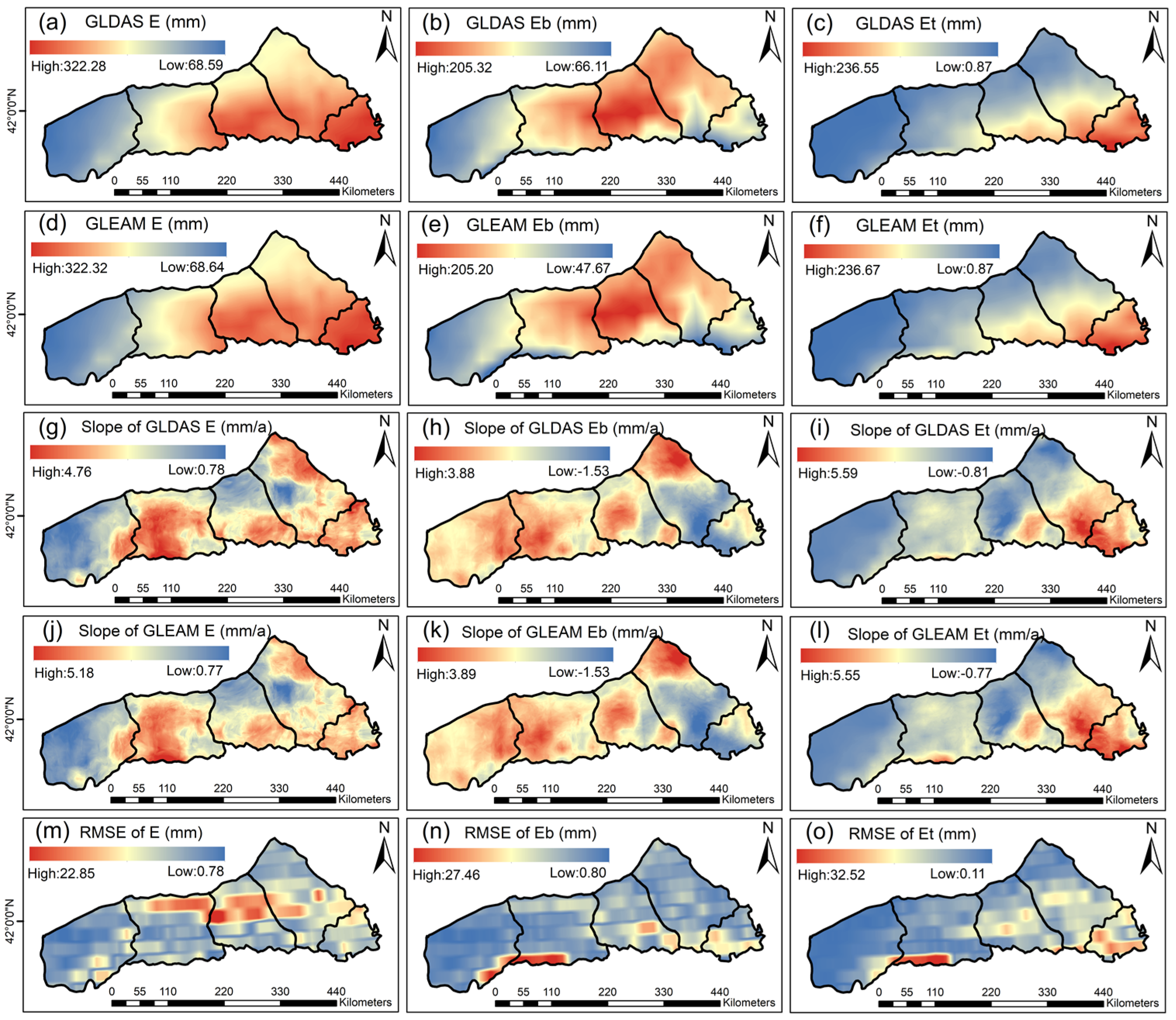
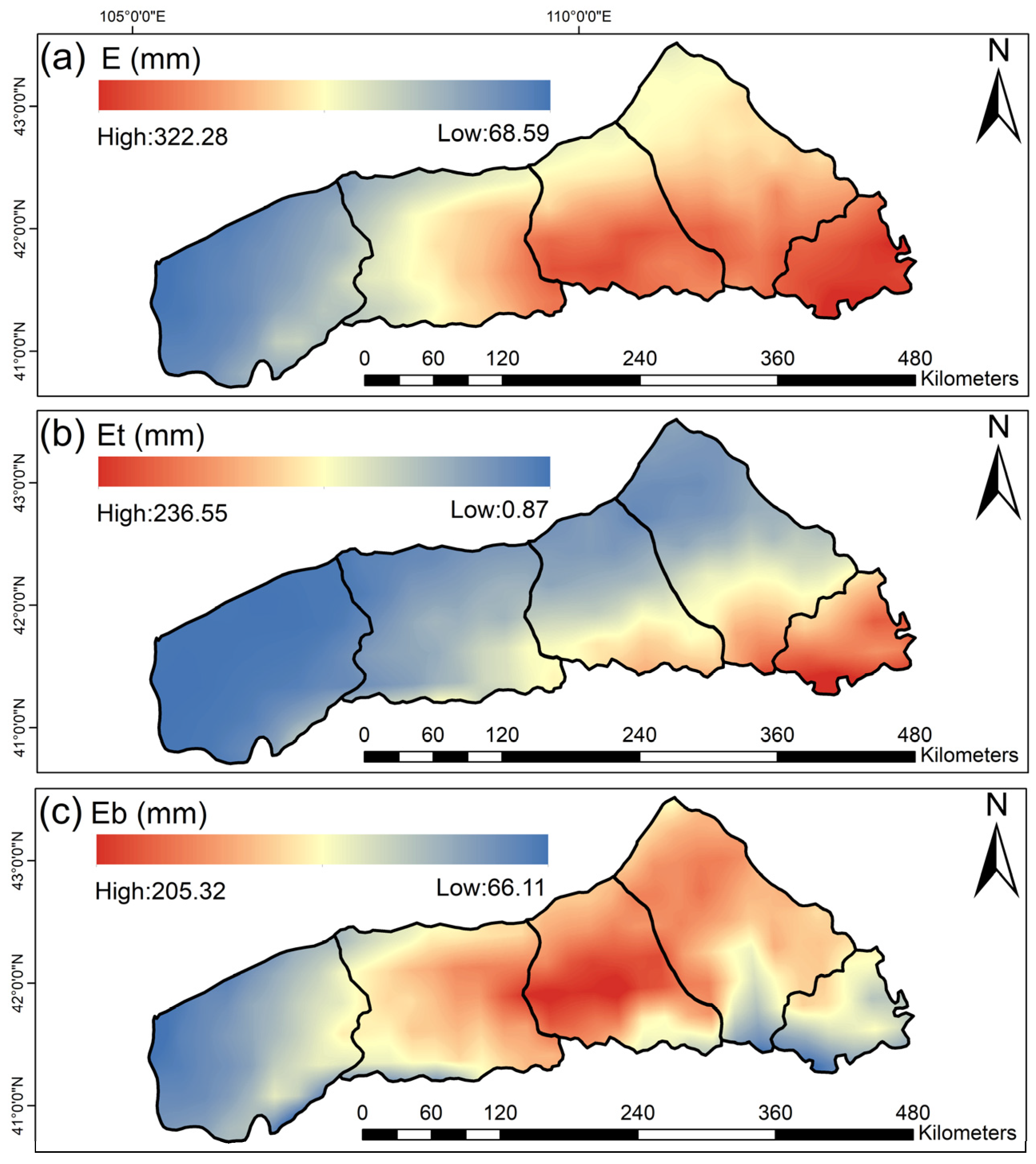
In time, E (2.47 mm/a, p < 0.01), Et (1.30 mm/a, p < 0.01), and Eb (1.06 mm/a, p < 0.01) all exhibited a significant upward trend. Spatially, the annual mean E decreased from the east (322.28 mm) to the west (68.59 mm), Et increased from the southeast (0.87 mm) to the northwest (236.55 mm), and Eb decreased from the northeast (205.32 mm) to the southwest (66.11 mm).

(2)

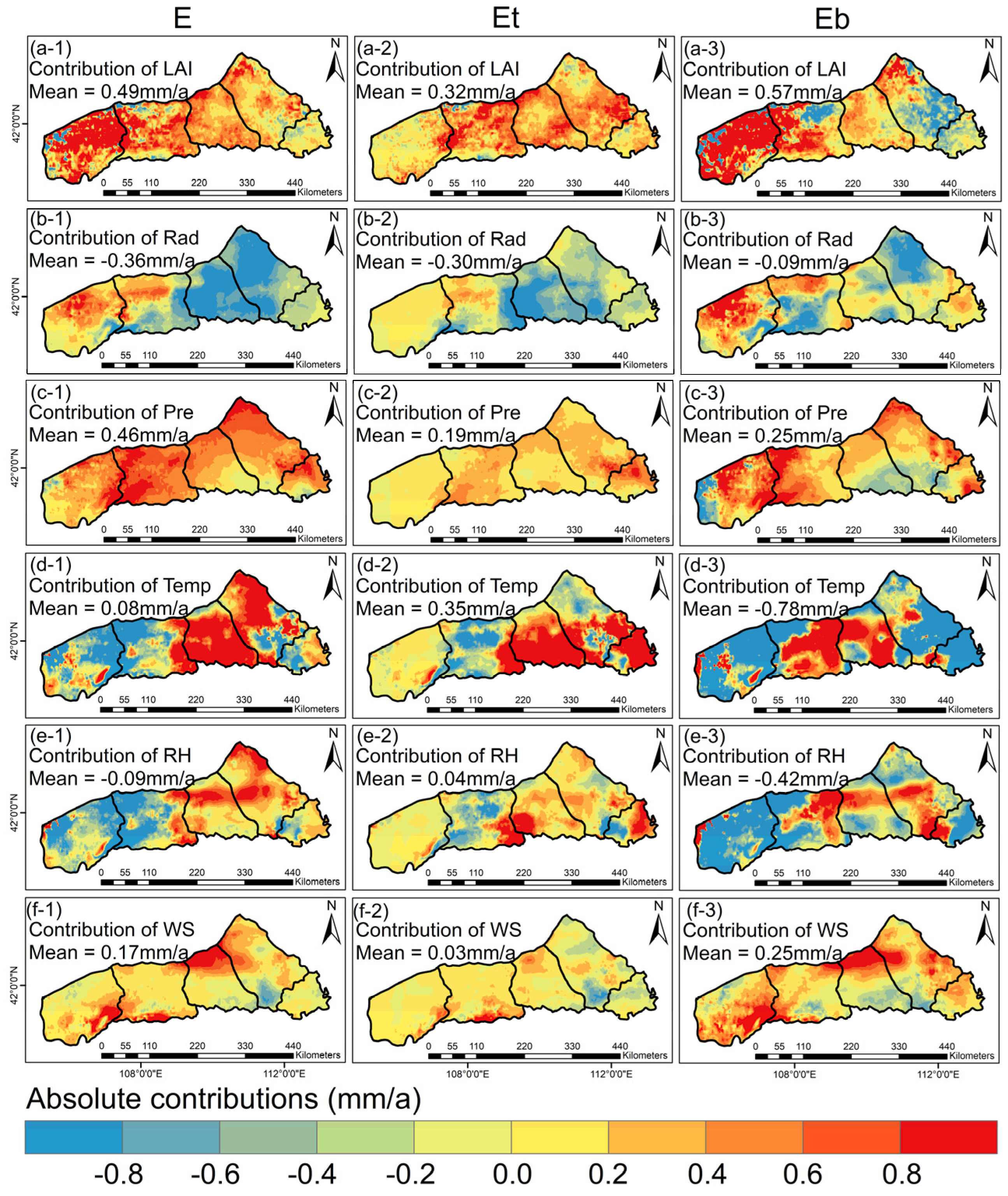
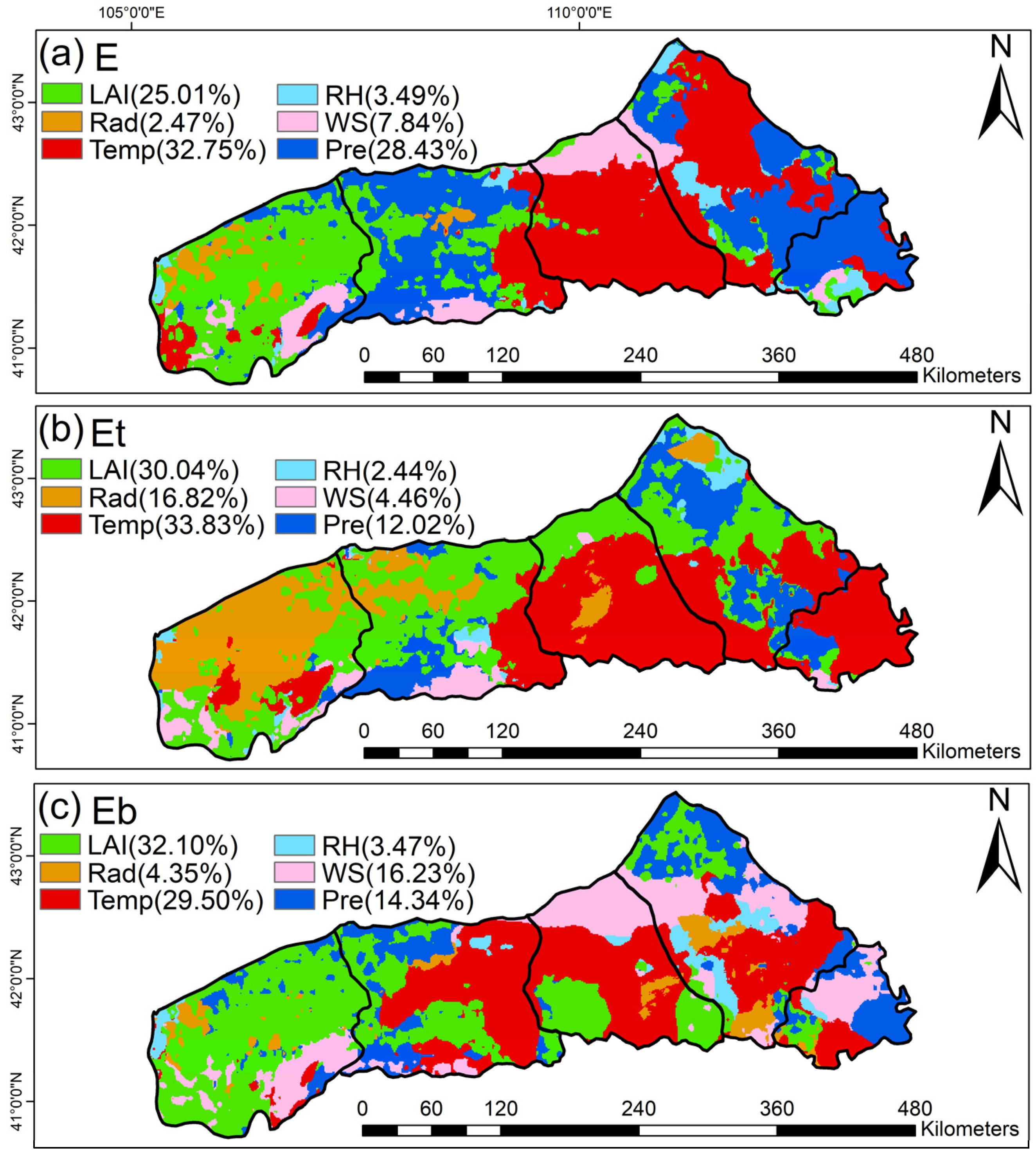
Vegetation greening emerges as the predominant impetus underpinning the augmentation of both E and Eb, augmenting their rates by 0.49 mm/a and 0.57 mm/a, respectively. For meteorological variables, Pre exerts the most conspicuous influence upon E (0.46 mm/a). Meanwhile, Temp emerges as the paramount determinant affecting Eb (−0.78 mm/a). Within the realm of Et, meteorological factors emerge as the primary catalysts, with Temp assuming a predominant role by augmenting Et at a rate of 0.35 mm/a. The contribution stemming from vegetation greening to Et is quantified at 0.32 mm/a. In addition, Pre always acts indirectly on E, Et, and Eb through its influence on other factors. Within E, Temp dominated in an area covering 32.75% of the study region. For Et, Temp had the highest dominance, covering 33.83% of the study area. For Eb, the main controlling factors were LAI (32.10%) and Temp (29.50%).

(3)

LAI often acted as an intermediary variable between RH, WS, and Pre on E and its components. LAI had a direct path coefficient on Et of 0.22 (p < 0.05). In addition to the direct effect of Pre on E (0.75, p < 0.01) and Et (0.51, p < 0.01), it also had an indirect effect (0.20, p < 0.05 and 0.39, p < 0.01, respectively). The indirect effect of Temp on Eb was more significant (−0.13, p < 0.05), while Rad mainly had a direct effect on Eb (−0.21, p < 0.05).

Through comprehensive ecological management, the effective control and restoration of degraded forests and grasslands has been achieved in the current stage within the region. The foundational framework of an important ecological security barrier in the NFYM is essentially established. These findings offer valuable insights to local governments for the formulation of sustainable water resource and vegetation restoration strategies.

References

1. Zhang, K.; Kimball, J.S.; Running, S.W. A review of remote sensing based actual evapotranspiration estimation. Wiley Interdiscip. Rev. Water 2016, 3, 834–853. [Google Scholar] [CrossRef]
2. L’Ecuyer, T.S.; Beaudoing, H.K.; Rodell, M.; Olson, W.; Lin, B.; Kato, S.; Clayson, C.A.; Wood, E.; Sheffield, J.; Adler, R.; et al. The Observed State of the Energy Budget in the Early Twenty-First Century. J. Clim. 2015, 28, 8319–8346. [Google Scholar] [CrossRef]
3. Trenberth, K.E.; Smith, L.; Qian, T.T.; Dai, A.; Fasullo, J. Estimates of the global water budget and its annual cycle using observational and model data. J. Hydrometeorol. 2007, 8, 758–769. [Google Scholar] [CrossRef]
4. Sun, S.L.; Liu, Y.B.; Chen, H.S.; Ju, W.M.; Xu, C.Y.; Liu, Y.; Zhou, B.T.; Zhou, Y.; Zhou, Y.L.; Yu, M. Causes for the increases in both evapotranspiration and water yield over vegetated mainland China during the last two decades. Agric. For. Meteorol. 2022, 324, 109118. [Google Scholar] [CrossRef]
5. Niu, Z.G.; He, H.L.; Zhu, G.F.; Ren, X.L.; Zhang, L.; Zhang, K.; Yu, G.R.; Ge, R.; Li, P.; Zeng, N.; et al. An increasing trend in the ratio of transpiration to total terrestrial evapotranspiration in China from 1982 to 2015 caused by greening and warming. Agric. For. Meteorol. 2019, 279, 107701. [Google Scholar] [CrossRef]
6. Elbeltagi, A.; Kumari, N.; Dharpure, J.K.; Mokhtar, A.; Alsafadi, K.; Kumar, M.; Mehdinejadiani, B.; Etedali, H.R.; Brouziyne, Y.; Islam, A.M.T.; et al. Prediction of Combined Terrestrial Evapotranspiration Index (CTEI) over Large River Basin Based on Machine Learning Approaches. Water 2021, 13, 547. [Google Scholar] [CrossRef]
7. Fisher, J.B.; Melton, F.; Middleton, E.; Hain, C.; Anderson, M.; Allen, R.; McCabe, M.F.; Hook, S.; Baldocchi, D.; Townsend, P.A.; et al. The future of evapotranspiration: Global requirements for ecosystem functioning, carbon and climate feedbacks, agricultural management, and water resources. Water Resour. Res. 2017, 53, 2618–2626. [Google Scholar] [CrossRef]
8. Lee, S.J.; Kim, N.; Lee, Y. Development of Integrated Crop Drought Index by Combining Rainfall, Land Surface Temperature, Evapotranspiration, Soil Moisture, and Vegetation Index for Agricultural Drought Monitoring. Remote Sens. 2021, 13, 1778. [Google Scholar] [CrossRef]
9. Cheng, L.Z.; Yang, M.X.; Wang, X.J.; Wan, G.N. Spatial and Temporal Variations of Terrestrial Evapotranspiration in the Upper Taohe River Basin from 2001 to 2018 Based on MOD16 ET Data. Adv. Meteorol. 2020, 2020, 3721414. [Google Scholar] [CrossRef]
10. Cheng, M.H.; Jiao, X.Y.; Jin, X.L.; Li, B.B.; Liu, K.H.; Shi, L. Satellite time series data reveal interannual and seasonal spatiotemporal evapotranspiration patterns in China in response to effect factors. Agric. Water Manag. 2021, 255, 107046. [Google Scholar] [CrossRef]
11. Pascolini-Campbell, M.; Reager, J.T.; Chandanpurkar, H.A.; Rodell, M. A 10 percent increase in global land evapotranspiration from 2003 to 2019. Nature 2021, 593, 543–547. [Google Scholar] [CrossRef] [PubMed]
12. Baldocchi, D.; Falge, E.; Gu, L.H.; Olson, R.; Hollinger, D.; Running, S.; Anthoni, P.; Bernhofer, C.; Davis, K.; Evans, R.; et al. FLUXNET: A new tool to study the temporal and spatial variability of ecosystem-scale carbon dioxide, water vapor, and energy flux densities. Bull. Am. Meteorol. Soc. 2001, 82, 2415–2434. [Google Scholar] [CrossRef]
13. Jung, M.; Koirala, S.; Weber, U.; Ichii, K.; Gans, F.; Camps-Valls, G.; Papale, D.; Schwalm, C.; Tramontana, G.; Reichstein, M. The FLUXCOM ensemble of global land-atmosphere energy fluxes. Sci. Data 2019, 6, 74. [Google Scholar] [CrossRef] [PubMed]
14. Chen, H.; Huang, J.H.J.; McBean, E.; Singh, V.P. Evaluation of alternative two-source remote sensing models in partitioning of land evapotranspiration. J. Hydrol. 2021, 597, 126029. [Google Scholar] [CrossRef]
15. Cui, Y.K.; Song, L.S.; Fan, W.J. Generation of spatio-temporally continuous evapotranspiration and its components by coupling a two-source energy balance model and a deep neural network over the Heihe River Basin. J. Hydrol. 2021, 597, 126176. [Google Scholar] [CrossRef]
16. Yang, Y.; Guan, K.Y.; Peng, B.; Pan, M.; Jiang, C.Y.; Franz, T.E. High-resolution spatially explicit land surface model calibration using field-scale satellite-based daily evapotranspiration product. J. Hydrol. 2021, 596, 125730. [Google Scholar] [CrossRef]
17. Mu, Q.; Heinsch, F.A.; Zhao, M.; Running, S.W. Development of a global evapotranspiration algorithm based on MODIS and global meteorology data. Remote Sens. Environ. 2007, 111, 519–536. [Google Scholar] [CrossRef]
18. Mu, Q.Z.; Zhao, M.S.; Running, S.W. Improvements to a MODIS global terrestrial evapotranspiration algorithm. Remote Sens. Environ. 2011, 115, 1781–1800. [Google Scholar] [CrossRef]
19. Yang, X.Q.; Yong, B.; Ren, L.L.; Zhang, Y.Q.; Long, D. Multi-scale validation of GLEAM evapotranspiration products over China via ChinaFLUX ET measurements. Int. J. Remote Sens. 2017, 38, 5688–5709. [Google Scholar] [CrossRef]
20. Baik, J.; Choi, M. Multi-satellite-based water budget components in South Korea. Environ. Earth Sci. 2018, 77, 93. [Google Scholar] [CrossRef]
21. Feng, Y.; Cui, N.B.; Zhao, L.; Gong, D.Z.; Zhang, K.D. Spatiotemporal variation of reference evapotranspiration during 1954–2013 in Southwest China. Quat. Int. 2017, 441, 129–139. [Google Scholar] [CrossRef]
22. Zhang, S.L.; Yang, H.B.; Yang, D.W.; Jayawardena, A.W. Quantifying the effect of vegetation change on the regional water balance within the Budyko framework. Geophys. Res. Lett. 2016, 43, 1140–1148. [Google Scholar] [CrossRef]
23. Schlaepfer, D.R.; Ewers, B.E.; Shuman, B.N.; Williams, D.G.; Frank, J.M.; Massman, W.J.; Lauenroth, W.K. Terrestrial water fluxes dominated by transpiration: Comment. Ecosphere 2014, 5, 1–9. [Google Scholar] [CrossRef]
24. Lian, X.; Piao, S.L.; Huntingford, C.; Li, Y.; Zeng, Z.Z.; Wang, X.H.; Ciais, P.; McVicar, T.R.; Peng, S.S.; Ottle, C.; et al. Partitioning global land evapotranspiration using CMIP5 models constrained by observations. Nat. Clim. Chang. 2018, 8, 640–646. [Google Scholar] [CrossRef]
25. Porada, P.; Van Stan, J.T.; Kleidon, A. Significant contribution of non-vascular vegetation to global rainfall interception. Nat. Geosci. 2018, 11, 563–567. [Google Scholar] [CrossRef]
26. Zhang, Y.Q.; Pena-Arancibia, J.L.; McVicar, T.R.; Chiew, F.H.S.; Vaze, J.; Liu, C.M.; Lu, X.J.; Zheng, H.X.; Wang, Y.P.; Liu, Y.Y.; et al. Multi-decadal trends in global terrestrial evapotranspiration and its components. Sci. Rep. 2016, 6, 19124. [Google Scholar] [CrossRef] [PubMed]
27. Costa, M.H.; Biajoli, M.C.; Sanches, L.; Malhado, A.C.M.; Hutyra, L.R.; da Rocha, H.R.; Aguiar, R.G.; de Araujo, A.C. Atmospheric versus vegetation controls of Amazonian tropical rain forest evapotranspiration: Are the wet and seasonally dry rain forests any different? J. Geophys. Res. Biogeosci. 2010, 115, G04021. [Google Scholar] [CrossRef]
28. Kukal, M.; Irmak, S. Long-term patterns of air temperatures, daily temperature range, precipitation, grass-reference evapotranspiration and aridity index in the USA great plains: Part II. Temporal trends. J. Hydrol. 2016, 542, 978–1001. [Google Scholar] [CrossRef]
29. Adeyeri, O.E.; Ishola, K.A. Variability and Trends of Actual Evapotranspiration over West Africa: The Role of Environmental Drivers. Agric. For. Meteorol. 2021, 308, 108574. [Google Scholar] [CrossRef]
30. Skliris, N.; Zika, J.D.; Nurser, G.; Josey, S.A.; Marsh, R. Global water cycle amplifying at less than the Clausius-Clapeyron rate. Sci. Rep. 2016, 6, 38752. [Google Scholar] [CrossRef]
31. Trebs, I.; Mallick, K.; Bhattarai, N.; Sulis, M.; Cleverly, J.; Woodgate, W.; Silberstein, R.; Hinko-Najera, N.; Beringer, J.; Meyer, W.S.; et al. The role of aerodynamic resistance in thermal remote sensing-based evapotranspiration models. Remote Sens. Environ. 2021, 264, 112602. [Google Scholar] [CrossRef]
32. Duo, A.; Zhao, W.J.; Qua, X.Y.; Jing, R.; Xiong, K. Spatio-temporal variation of vegetation coverage and its response to climate change in North China plain in the last 33 years. Int. J. Appl. Earth Obs. Geoinformat. 2016, 53, 103–117. [Google Scholar] [CrossRef]
33. Sun, G.; Caldwell, P.V.; McNulty, S.G. Modelling the potential role of forest thinning in maintaining water supplies under a changing climate across the conterminous United States. Hydrol. Process. 2015, 29, 5016–5030. [Google Scholar] [CrossRef]
34. Jin, Z.; Liang, W.; Yang, Y.T.; Zhang, W.B.; Yan, J.W.; Chen, X.J.; Li, S.; Mo, X.G. Separating Vegetation Greening and Climate Change Controls on Evapotranspiration trend over the Loess Plateau. Sci. Rep. 2017, 7, 8191. [Google Scholar] [CrossRef] [PubMed]
35. Mo, X.G.; Chen, X.J.; Hu, S.; Liu, S.X.; Xia, J. Attributing regional trends of evapotranspiration and gross primary productivity with remote sensing: A case study in the North China Plain. Hydrol. Earth Syst. Sci. 2017, 21, 295–310. [Google Scholar] [CrossRef]
36. Zhao, F.B.; Ma, S.; Wu, Y.P.; Qiu, L.J.; Wang, W.K.; Lian, Y.Q.; Chen, J.; Sivakumar, B. The role of climate change and vegetation greening on evapotranspiration variation in the Yellow River Basin, China. Agric. For. Meteorol. 2022, 316, 108842. [Google Scholar] [CrossRef]
37. Deng, C.L.; Zhang, B.Q.; Cheng, L.Y.; Hu, L.Q.; Chen, F.H. Vegetation dynamics and their effects on surface water-energy balance over the Three-North Region of China. Agric. For. Meteorol. 2019, 275, 79–90. [Google Scholar] [CrossRef]
38. Xue, Y.; Liang, H.; Zhang, H.; Yin, L.; Feng, X. Quantifying the policy-driven large scale vegetation restoration effects on evapotranspiration over drylands in China. J. Environ. Manag. 2023, 345, 118723. [Google Scholar] [CrossRef]
39. Zhang, Y.Q.; Kong, D.D.; Gan, R.; Chiew, F.H.S.; McVicar, T.R.; Zhang, Q.; Yang, Y.T. Coupled estimation of 500 m and 8-day resolution global evapotranspiration and gross primary production in 2002–2017. Remote Sens. Environ. 2019, 222, 165–182. [Google Scholar] [CrossRef]
40. Khan, M.S.; Liaqat, U.W.; Baik, J.; Choi, M. Stand-alone uncertainty characterization of GLEAM, GLDAS and MOD16 evapotranspiration products using an extended triple collocation approach. Agric. For. Meteorol. 2018, 252, 256–268. [Google Scholar] [CrossRef]
41. Wang, W.; Cui, W.; Wang, X.J.; Chen, X. Evaluation of GLDAS-1 and GLDAS-2 Forcing Data and Noah Model Simulations over China at the Monthly Scale. J. Hydrometeorol. 2016, 17, 2815–2833. [Google Scholar] [CrossRef]
42. Liu, Y.Y.; Lin, Z.Q.; Wang, Z.J.; Chen, X.; Han, P.D.; Wang, B.; Wang, Z.Q.; Wen, Z.M.; Shi, H.J.; Zhang, Z.X.; et al. Discriminating the impacts of vegetation greening and climate change on the changes in evapotranspiration and transpiration fraction over the Yellow River Basin. Sci. Total Environ. 2023, 904, 166926. [Google Scholar] [CrossRef] [PubMed]
43. Wang, L.X.; Good, S.P.; Caylor, K.K. Global synthesis of vegetation control on evapotranspiration partitioning. Geophys. Res. Lett. 2014, 41, 6753–6757. [Google Scholar] [CrossRef]
44. Zeng, Z.Z.; Piao, S.L.; Li, L.Z.X.; Zhou, L.M.; Ciais, P.; Wang, T.; Li, Y.; Lian, X.; Wood, E.F.; Friedlingstein, P.; et al. Climate mitigation from vegetation biophysical feedbacks during the past three decades. Nat. Clim. Chang. 2017, 7, 432–436. [Google Scholar] [CrossRef]
45. Wei, Z.W.; Yoshimura, K.; Wang, L.X.; Miralles, D.G.; Jasechko, S.; Lee, X.H. Revisiting the contribution of transpiration to global terrestrial evapotranspiration. Geophys. Res. Lett. 2017, 44, 2792–2801. [Google Scholar] [CrossRef]
46. Yang, J.; Huang, X. The 30 m annual land cover dataset and its dynamics in China from 1990 to 2019. Earth Syst. Sci. Data 2021, 13, 3907–3925. [Google Scholar] [CrossRef]
47. Terán, C.P.; Naz, B.S.; Graf, A.; Qu, Y.Q.; Franssen, H.J.H.; Baatz, R.; Ciais, P.; Vereecken, H. Rising water-use efficiency in European grasslands is driven by increased primary production. Commun. Earth Environ. 2023, 4, 95. [Google Scholar] [CrossRef]
48. Yang, S.S.; Zhang, J.H.; Han, J.Q.; Wang, J.W.; Zhang, S.; Bai, Y.; Cao, D.; Xun, L.; Zheng, M.X.; Chen, H.; et al. Evaluating global ecosystem water use efficiency response to drought based on multi-model analysis. Sci. Total Environ. 2021, 778, 146356. [Google Scholar] [CrossRef]
49. Yang, X.Y.; Zhang, Z.P.; Guan, Q.Y.; Zhang, E.; Sun, Y.F.; Yan, Y.; Du, Q.Q. Coupling mechanism between vegetation and multi-depth soil moisture in arid-semiarid area: Shift of dominant role from vegetation to soil moisture. For. Ecol. Manag. 2023, 546, 121323. [Google Scholar] [CrossRef]
50. Zhao, Y.; Chen, Y.A.; Wu, C.Y.; Li, G.; Ma, M.G.; Fan, L.; Zheng, H.; Song, L.S.; Tang, X.G. Exploring the contribution of environmental factors to evapotranspiration dynamics in the Three-River-Source region, China. J. Hydrol. 2023, 626, 130222. [Google Scholar] [CrossRef]
51. Chen, X.J.; Mo, X.G.; Hu, S.; Liu, S.X. Contributions of climate change and human activities to ET and GPP trends over North China Plain from 2000 to 2014. J. Geogr. Sci. 2017, 27, 661–680. [Google Scholar] [CrossRef]
52. Li, X.Y.; Zou, L.; Xia, J.; Dou, M.; Li, H.W.; Song, Z.H. Untangling the effects of climate change and land use/cover change on spatiotemporal variation of evapotranspiration over China. J. Hydrol. 2022, 612, 128189. [Google Scholar] [CrossRef]
53. Roderick, M.L.; Rotstayn, L.D.; Farquhar, G.D.; Hobbins, M.T. On the attribution of changing pan evaporation. Geophys. Res. Lett. 2007, 34, L17403. [Google Scholar] [CrossRef]
54. Ye, X.C.; Li, X.H.; Liu, J.; Xu, C.Y.; Zhang, Q. Variation of reference evapotranspiration and its contributing climatic factors in the Poyang Lake catchment, China. Hydrol. Process. 2014, 28, 6151–6162. [Google Scholar] [CrossRef]
55. Abel, S.; Gislum, R.; Boelt, B. Path and correlation analysis of perennial ryegrass (Lolium perenne L.) seed yield components. J. Agron. Crop Sci. 2017, 203, 338–344. [Google Scholar] [CrossRef]
56. Yu, S.W.; Zhu, K.J.; Zhang, X. Energy demand projection of China using a path-coefficient analysis and PSO-GA approach. Energy Convers. Manag. 2012, 53, 142–153. [Google Scholar] [CrossRef]
57. Zhang, B.Z.; Xu, D.; Liu, Y.; Li, F.S.; Cai, J.B.; Du, L.J. Multi-scale evapotranspiration of summer maize and the controlling meteorological factors in north China. Agric. For. Meteorol. 2016, 216, 1–12. [Google Scholar] [CrossRef]
58. Ebrahimi, E.; Bayat, H.; Fallah, M. Relationship of soil moisture characteristic curve and mechanical properties in Entisols and Inceptisols of Iran. Geoderma Reg. 2021, 27, e00434. [Google Scholar] [CrossRef]
59. Hou, E.Q.; Chen, C.R.; Luo, Y.Q.; Zhou, G.Y.; Kuang, Y.W.; Zhang, Y.G.; Heenan, M.; Lu, X.K.; Wen, D.Z. Effects of climate on soil phosphorus cycle and availability in natural terrestrial ecosystems. Glob. Chang. Biol. 2018, 24, 3344–3356. [Google Scholar] [CrossRef]
60. Rosseel, Y. lavaan: An R Package for Structural Equation Modeling. J. Stat. Softw. 2012, 48, 1–36. [Google Scholar] [CrossRef]
61. Wang, C.Y.; Chen, J.; Gu, L.; Wu, G.Y.; Tong, S.L.; Xiong, L.H.; Xu, C.Y. A pathway analysis method for quantifying the contributions of precipitation and potential evapotranspiration anomalies to soil moisture drought. J. Hydrol. 2023, 621, 129570. [Google Scholar] [CrossRef]
62. Li, D.H.; Liu, K.; Wang, S.D.; Wu, T.X.; Li, H.; Bo, Y.; Zhang, H.Y.; Huang, Y.L.; Li, X.K. Four decades of hydrological response to vegetation dynamics and anthropogenic factors in the Three-North Region of China and Mongolia. Sci. Total Environ. 2023, 857, 159546. [Google Scholar] [CrossRef] [PubMed]
63. Cailliau, M.; Foresti, M.; Villar, C.M. Winds of Change. IEEE Power Energy Mag. 2010, 8, 53–62. [Google Scholar] [CrossRef]
64. Xu, J.M.; Wu, B.F.; Ryu, D.; Yan, N.N.; Zhu, W.W.; Ma, Z.H. A canopy conductance model with temporal physiological and environmental factors. Sci. Total Environ. 2021, 791, 148283. [Google Scholar] [CrossRef] [PubMed]
65. Chattopadhyay, N.; Hulme, M. Evaporation and potential evapotranspiration in India under conditions of recent and future climate change. Agric. For. Meteorol. 1997, 87, 55–73. [Google Scholar] [CrossRef]
66. Barnett, T.P.; Adam, J.C.; Lettenmaier, D.P. Potential impacts of a warming climate on water availability in snow-dominated regions. Nature 2005, 438, 303–309. [Google Scholar] [CrossRef]
67. Murray-Tortarolo, G.; Friedlingstein, P.; Sitch, S.; Seneviratne, S.I.; Fletcher, I.; Mueller, B.; Greve, P.; Anav, A.; Liu, Y.; Ahlstrom, A.; et al. The dry season intensity as a key driver of NPP trends. Geophys. Res. Lett. 2016, 43, 2632–2639. [Google Scholar] [CrossRef]
68. Caldwell, P.V.; Kennen, J.G.; Sun, G.; Kiang, J.E.; Butcher, J.B.; Eddy, M.C.; Hay, L.E.; LaFontaine, J.H.; Hain, E.F.; Nelson, S.A.C.; et al. A comparison of hydrologic models for ecological flows and water availability. Ecohydrology 2015, 8, 1525–1546. [Google Scholar] [CrossRef]
69. Cao, S.X.; Chen, L.; Shankman, D.; Wang, C.M.; Wang, X.B.; Zhang, H. Excessive reliance on afforestation in China’s arid and semi-arid regions: Lessons in ecological restoration. Earth-Sci. Rev. 2011, 104, 240–245. [Google Scholar] [CrossRef]
70. Tian, F.; Lu, Y.H.; Fu, B.J.; Zhang, L.; Zang, C.F.; Yang, Y.H.; Qiu, G.Y. Challenge of vegetation greening on water resources sustainability: Insights from a modeling-based analysis in Northwest China. Hydrol. Process. 2017, 31, 1469–1478. [Google Scholar] [CrossRef]
71. Bai, P.; Liu, X.M.; Zhang, Y.Q.; Liu, C.M. Assessing the Impacts of Vegetation Greenness Change on Evapotranspiration and Water Yield in China. Water Resour. Res. 2020, 56, e2019wr027019. [Google Scholar] [CrossRef]
72. Xie, S.D.; Mo, X.G.; Hu, S.; Liu, S.X. Contributions of climate change, elevated atmospheric CO2 and human activities to ET and GPP trends in the Three-North Region of China. Agric. For. Meteorol. 2020, 295, 108183. [Google Scholar] [CrossRef]
73. Shen, M.G.; Piao, S.L.; Jeong, S.J.; Zhou, L.M.; Zeng, Z.Z.; Ciais, P.; Chen, D.L.; Huang, M.T.; Jin, C.S.; Li, L.Z.X.; et al. Evaporative cooling over the Tibetan Plateau induced by vegetation growth. Proc. Natl. Acad. Sci. USA 2015, 112, 9299–9304. [Google Scholar] [CrossRef] [PubMed]
74. Ge, J.; Liu, Q.; Zan, B.L.; Lin, Z.Q.; Lu, S.; Qiu, B.; Guo, W.D. Deforestation intensifies daily temperature variability in the northern extratropics. Nat. Commun. 2022, 13, 5955. [Google Scholar] [CrossRef]
Figure 1. Study area. (a) Location, (b) elevation, and (c) land use/land cover types.
Remotesensing 16 00357 g001
Figure 2. Time trend of E and its components. (a) Time series of E and its components from 2000 to 2020; (bd) represent the mutation trends of E, Et, and Eb, respectively.
Remotesensing 16 00357 g002
Figure 3. Spatial distribution characteristics of annual average (a) E, (b) Et, and (c) Eb in NFYM from 2000 to 2020.
Remotesensing 16 00357 g003
Figure 4. Spatial patterns and significance tests of the changes in E and its components within the NFYM from 2000 to 2020 ((ac) represent E, Et, and Eb, respectively; 1 represents spatial patterns of change trends, 2 represents significance tests).
Remotesensing 16 00357 g004
Figure 5. Time trend of LAI. (a) represents the LAI time series from 2000 to 2020; (b) represents the LAI mutation trend.
Remotesensing 16 00357 g005
Figure 6. Time trends of climate variables. (a) Radiation, (b) Precipitation, (c) Temperature, (d) Relative Humidity, and (e) Wind Speed; 1 represents the time series of climate variables from 2000 to 2020, and 2 represents the abrupt change trend of climate variables.
Remotesensing 16 00357 g006
Figure 7. Spatial patterns and significance testing of LAI trends in the NFYM from 2000 to 2020. (a) represents spatial distribution characteristics of the annual average, (b) represents spatial patterns of trend changes, and (c) represents significance tests.
Remotesensing 16 00357 g007
Figure 8. Spatial distribution characteristics of annual average Rad (a), Pre (b), Temp (c), RH (d), and WS (e) in the NFYM from 2000 to 2020.
Remotesensing 16 00357 g008
Figure 9. Spatial patterns and significance testing of climate variable trends in the NFYM from 2000 to 2020. (ae) represent Rad, Pre, Temp, RH, and WS, respectively; 1 represents spatial patterns of trend changes, and 2 represents significance tests.
Remotesensing 16 00357 g009
Figure 10. Spatial distribution patterns of partial correlation coefficients (PCC) of driving factors for component E in the NFYM from 2000 to 2020. (a) LAI, (b) Rad, (c) Pre, (d) Temp, (e) RH, and (f) WS. 1 represents E, 2 represents Et, and 3 represents Eb.
Remotesensing 16 00357 g010
Figure 11. Spatial patterns of the absolute contributions of vegetation LAI and climate factors to the variations in E and its components. (a) LAI, (b) Rad, (c) Pre, (d) Temp, (e) RH, and (f) WS. 1 represents E, 2 represents Et, and 3 represents Eb.
Remotesensing 16 00357 g011
Figure 12. Spatial distribution characteristics of the dominant factors of the variation in area (a) E, (b) Et and (c) Eb from 2000 to 2020.
Remotesensing 16 00357 g012
Figure 13. Path analysis of (a) E, (b) Et, and (c) Eb. Standardized path coefficients less than 0.2 are connected by thin lines, standardized path coefficients between 0.2 and 0.4 are connected by medium-thick lines, and standardized path coefficients greater than 0.4 are connected by thick lines. Solid green arrows represent significant positive effects, solid gray arrows represent non-significant positive effects, dashed pink arrows represent significant negative effects, and dashed gray arrows represent non-significant negative effects. * indicates significance (* p < 0.05 and ** p < 0.01)).
Remotesensing 16 00357 g013