Abstract
Quasi-continuous wave radar is an attempt to give consideration to the performance of pulse and continuous wave radar signals. However, it also has the shortcomings of both. This paper aims to add a new quasi-continuous-wave coding method to the spaceborne synthetic aperture radar (SAR) system. The technology of improving spaceborne SAR imaging performance by coding quasi-continuous-wave pulses is studied, and some shortcomings of this algorithm are improved. Firstly, the application of quasi-continuous-wave radar in the SAR system is studied, and the coding and reconstruction scheme is provided so that this technology can be successfully applied in spaceborne SAR. Secondly, the effects of different quasi-continuous-wave coding methods on SAR imaging performance are evaluated, including signal-to-noise ratio, resolution, and integration time. Then, several coding schemes are given, and the characteristic changes of the signal after quasi-continuous-wave coding are analyzed. The transmit–receive conversion loss function and azimuth Doppler ambiguity function of the design scheme are analyzed, which proves the advantages of the scheme. Finally, we design the hardware implementation scheme and carry out the practical test.
1. Introduction
Quasi-continuous wave radar is a new radar system that has the advantages of both continuous wave radar and pulse radar [1]. It uses pulse waveform with a working ratio close to 50%, which solves the problem of transmitting and receiving isolation of continuous wave radar, increases the operating range of radar, and overcomes the shortcomings of high peak power of pulse radar, with low interception rate and anti-active jamming ability.
Its advantage lies in the method of truncating the phase-modulated continuous-wave (CW) signal with appropriate sequence to form a large-time wideband wide-product expanded spectrum signal, which not only retains the main advantages of CW radar, but also has high range and velocity resolution and solves the problem of transmit–receive isolation of CW radar [1]. Due to the large duration of the signal, the coherent processing time of the radar can be increased, and the distant target can be found with lower radiation power. At the same detection distance, the transmitting power of this radar is low, so it has low interception probability performance and good electromagnetic compatibility. In receiver, it adopts the method of pseudo-code matching filter for correlation processing, and has a strong ability to resist active and passive interference [2]. To sum up, it has broad application prospects in both civil and military fields.
In the 1990s, western and domestic scholars put forward the concept of quasi-continuous-wave radar one after another [3,4], mainly focusing on waveform design and signal processing [5,6]. Russia started earlier in the research and application of quasi-continuous-wave radar, as early as the former Soviet Union published relevant monographs, and developed and installed space measurement radar using quasi-continuous-wave pulse waveform design [7]. The system uses the signal form that the width of the radiation pulse matches the distance of the target, makes full use of the maximum efficiency of the transmitting system, achieves a longer range with a smaller radar scale, and reduces the development cost of the system.
The St. Petersburg State Electrotechnical University of Russia has carried out long-term research on quasi-continuous-wave radar. Their research [8,9] uses phase-coded modulation and amplitude-modulated complex signal radar systems, which have specific applications in ocean target surveillance, ocean atmosphere monitoring, and equipment development. Memorial University of Newfoundland used linear frequency modulated interrupted continuous wave (LFM) signals for over-the-horizon (OTH) detection of sea surface targets [3,10]. Mcgregor used a single-antenna radar to conduct applied research on ocean wave and current monitoring [11]. In the study of ocean gravity waves at Wuhan University, linear frequency modulation to interrupt continuous wave radar is used to measure ocean gravity waves and ocean currents beyond visual range.
However, although quasi-continuous-wave radar makes the problem of transmit–receive isolation better, due to the receiving system being shut down during the transmission of the radar signal, the target echo in some distance segments (especially the short-range segment) cannot completely enter the radar receiver so that the target echo with good autocorrelation performance is truncated, which causes the target echo main sidelobe ratio to decrease seriously after pulse compression processing that affects the radar detection performance sometimes [12]. In rare cases, it is possible to make the radar unable to detect the target.
Therefore, it is very important to solve the ambiguity and occlusion problem of quasi-continuous-wave radar. Previously, the range occlusion problem of quasi-continuous-wave system radar was mostly studied from the angle of radar waveform design and parameter selection. In [13,14], a composite code based on optimal code and Gold code is proposed and applied to the waveform design of quasi-continuous-wave radar, effectively reducing the range occlusion probability of radar. In [15], poly-phase coding was used to design a quasi-continuous-wave radar waveform and optimize its peak side lobe ratio(PSRL) during distance occlusion, improving the detection performance of radar. In [16], they provide a solution to the echo occlusion problem from two aspects of waveform design and code design, but do not comprehensively consider the selection of waveform parameters. Figure 1 shows a schematic diagram of the occlusion and aliasing effect of the echo of a ship target observed by a quasi-continuous-waveform radar.
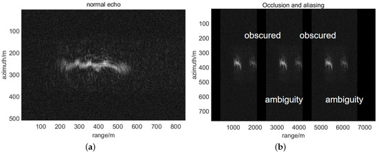
Figure 1.
(a) Normal observation echo of a ship. (b) Schematic of occluded and aliased echoes after quasi-continuous-wave observation of a ship.
Hong et al. proposed a periodic square wave discontinuous method instead of a sine frequency modulation method to solve the leakage problem of continuous wave [17]. This method is to set up a number of transceiver switches in the transceiver branch, and make the radar work in the quasi-continuous-wave mode under the control of a large-duty-cycle pulse signal. However, the continuous wave radar with periodic square wave discontinuous wave has periodic range blind spots, and there are some problems, such as velocity ambiguity and poor anti-interference performance at long operating distances. Therefore, they proposed another new continuous wave radar [18] with random code amplitude modulation and intermittent, and made a detailed analysis of the range equation. However, the random waveform does not consider the optimization of echo occlusion, and the distance occlusion probability is 0.5. There are some other methods to design low-probability radar waveforms [19]. Multi-channel SAR can alleviate this problem by introducing new equations [20,21,22,23]. There are fewer blind zones in multiple channels system. In theory, variational codes make variational blind zones and staggered blind zones are solvable [24].
None of them performed a signal fitting. By their nature, they are trying to minimize the probability of aliasing and occlusion, instead of solving them. So, our approach is completely different from the approaches of the others mentioned above. We allow occlusion and aliasing to occur, and control where they occur through coding, then reconstruct the echo through the corresponding decoding [1,25].
To sum up, the urgent problems to be solved in the application of quasi-continuous-wave coding detection in spaceborne SAR are coding design, occlusion and aliasing processing, and corresponding performance analysis.
2. Design for System Model
2.1. Principle
Quasi-continuous waveform coding detection is a method of cooperative detection that combines multiple transmitted pulses of radar. Among them, the number of transmitted pulses, pulse width, frequency bandwidth and the interval between pulses are combined and arranged according to the needs, which is called pulse coding [1,26]. The encoding method can be used in different forms according to the need, for example, the full-band pulse can be used to repeat the transmission many times. The original full-bandwidth single-pulse signal can also be divided into several partial bandwidth pulses and transmitted according to certain rules. The processing of synthesizing the intermittently received echo signal into a complete monopulse echo signal is called echo signal recovery [25]. The realization of pulse coding detection can be intuitively understood as converting an original transmitted pulse into a group of transmitted pulses for detection. This is equivalent to increasing the repetition rate of the transmitted pulse, which has the advantages of high duty cycle and average power, but it may also produce signal occlusion and aliasing problems, which affect the complete acquisition requirements of radar target information. Through the combination coding of multiple pulses, it provides a more flexible and advantageous implementation method for radar [25,27,28]. Different from the common monopulse radar, the radar multi-pulse combination detection needs to introduce the target signal recovery process [29,30]. The flow chart of the probe is shown in Figure 2.
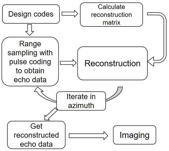
Figure 2.
Algorithm flow chart.
Radar pulse signals should be replaced by pulse coding combinations. As an example of a coded pulse set, we can write:
In the above statement, represents the subpulse waveform at position L. The subpulse widths are standardized as a single subpulse width, with no variation among them. Likewise, we standardize the pulse recurrence time (PRT), echo, and subaperture time by subpulse width in the following discussion. Depending on whether it emits or not, can be categorized into two types:
Assume that the echo length of our region of interest () is K, which is denoted by . Connect the echoes of all subpulses as a vector :
Echo is evidently a combination of all subpulse echoes obtained in the receiving window in a linear fashion:
The matrix serves as a representation of the observations we set up. It describes how every subpulse signal that is transmitted plays a role in a distinct receiving window. Its specific expression is as follows:
Now the problem is transformed into how to derive the observation matrix from . It can be derived from the physical meaning of : represents the observation matrix derived from the transmitted subpulse group , which is utilized to ascertain the contribution of every transmitted subpulse to distinct windows for received. Naturally, its dimension is determined by the number and total length of the observation windows of , where each value represents the observation state, which means “observed” and “not observed”. It is clear that A is a logical matrix.
Equation (6) determines the elements of the observation matrix .
where denotes the location of the m’th receiving window within . In the case where , it signifies that the n’th ideal echo is received within the m’th window.
The fitting estimated value of the echo matrix of the target can be derived from the linear relationship mentioned above.
Here signifies the outcome of the ideal echo reconstruction.
Under specific circumstances, it is possible to reconstruct the echoes of all subpulses, as indicated above. The existence of can be demonstrated when the end receiver window exceeds the length of K, because the raw material from which we fit the occluded echoes is the aliased echoes, we must ensure that all the information of the scene is completely acquired at least once during the whole detection time.
2.2. The Monopulse Group Model with Reduced Dimensionality under Approximate Conditions
In the event that several subpulses are placed in one , as the number of subpulses (set as M) increases, it becomes imperative to reconstruct a greater number of echoes. Finding the corresponding inverse matrix over time proves to be challenging. Nevertheless, in the case of linear correlation among the subechoes, the approximate relationship can be employed to streamline the computation [31]. The coding model for a single pulse is provided in the following manner.
Suppose that the transmission situation of the whole PRT including the subpulse coding is regarded as a whole coded , and the value of the transmitted subpulse is , and the value of the no transmitted subpulse is 0. For the kth echo window, the composition of the echo R is the kth row of multiplied by the ideal echo
where if indicates whether the current echo window can receive the echo with delay 1, so it mainly depends on whether the previous one of the kth echo window transmits the echo. Similarly, the second value indicates whether the ’th windows emitted an echo or not. If we denote the location of the kth receive window as , we can obtain all the values of .
It is worth noting that denotes the transmitted subpulse m positions ahead of the current position . Thus when , denotes the encoded value during the last PRT.
takes K values from the reverse cycle of the whole . Let denote the row vector (a row with K columns) obtained from by looping K values backward from the receiving window position , then
Since the distance between the satellite and the ground is far away, the round-return delay of the echo is generally larger than the , which is not the echo of the pulse in the current , but the echo of the previous pulse. However, if the whole is regarded as a complete coding, the correctness of (8) can be not affected. Suppose is the echo of a single pulse before n, the scene proximal and scene distal distances are and , respectively the corresponding delays are and :
where and correspond to the opening and closing time of the receiving gate of spaceborne SAR.
Equation (4) can still be used to express the relationship between the echo and that needs to be reconstructed, while the of constructor transforms into K.
Currently, the majority of the elements in matrix are empty. In the case of spaceborne SAR, there is no echo outside the range gate, thus necessitating the reconstruction of solely the effective component within the gate. In this particular instance, it is possible to make the reconstruction matrix more straightforward. The decomposition of the observation matrix and the ideal scene echo is as follows:
Now can be reduced to:
Now the problem is simplified as only the non-zero portion of the echo can be approximated. This part is estimated to be:
After the simplification operation, the amount of computation is significantly reduced. However, this method considers that the echoes of all subpulses are correlated with the first echo, while the satellite is moving at a great velocity. When imaging a wide range of scenes, the Doppler effect between each subpulse group can not be ignored in fact. Because of the manner in which radar data are sampled, the Doppler center frequency may be aliased, so its observed value is different from its absolute value. Therefore, only for a few small scene fast imaging tasks is it suitable to sacrifice resolution and total integration time for a large reduction in computational complexity.
3. Simulation and Experiment
3.1. Validation of Point Target Simulations
This section contains two parts of simulation validation. The first simulation uses ideal pulse-coded echoes to verify the feasibility of the pulse-coded reconstruction technique. The second simulation is carried out strictly according to the actual situation of spaceborne SAR application of pulse coding, including the difference between subpulse echoes, so as to observe the applicability of the theoretical premise of pulse coding in spaceborne SAR application [23].
Table 1 displays a part of system parameters that we set in the spaceborne SAR utilized in our test.

Table 1.
Parameters for the simulation.
We employed these system parameters to replicate the echo and image of the conventional technique, subsequently substituting the customary pulse with the meticulously crafted coding to obtain the echo for reconstruction.
The code is designed as follows:
The simulation of point and array targets is carried out. Figure 3 shows a comparison of SAR images obtained using conventional and pulse coding techniques. It can be seen that our method has the consistent imaging performance of traditional methods, which verifies the accuracy of our previous inferences and the rationality of our simplification in Section 2.2.
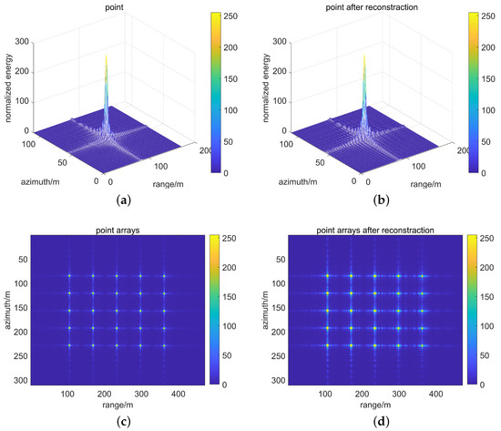
Figure 3.
(a) Point target; (b) point target after reconstruction; (c) point arrays; (d) point arrays after reconstruction.
Figure 3 verifies the correctness of the reconstruction theory and proves that the reconstruction can completely restore the occluded echo signal. However, it can also be seen that the reconstruction will affect the performance of the image. For example, compared with (a) and (b), azimuth has truncation error; compared with (c) and (d), the SNR of the reconstructed signal has changed. According to our testing, these performance changes are strongly correlated with the coding scheme, so we conduct a detailed evaluation of the impact of the coding scheme on the image performance subsequently.
3.2. Testing and Evaluation of Pulse Coding and Reconstruction
We use the sliding rail to simulate the orbit state of spaceborne SAR to establish a space model with equal scaling. The USS Abraham Lincoln model has been observed from 10 different angles, using traditional technology and quasi-continuous-wave coding technology (Figure 4). A sparser coding was adopted here.
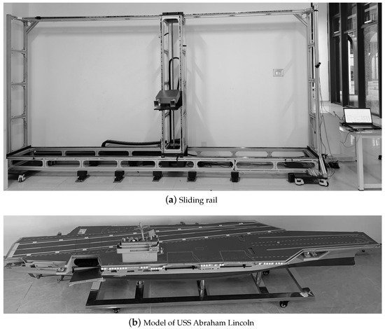
Figure 4.
Experimental site and props.
Some of the results are shown in Figure 5.
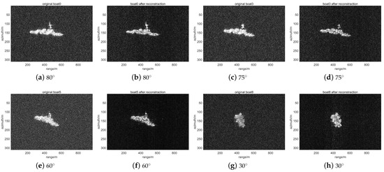
Figure 5.
Reconstructed images by pulse coding of ships from different angles compared with common images.
In conventional SAR, the radar antenna is pointed in a direction perpendicular to the velocity vector of the radar platform, i.e., in the side-looking position. As shown in Figure 5, (a,b) is the conventional view, (c,d) is the result of 30-degree angle squint observation, and (e,f) is the result of observation in the case of large noise interference. It can be seen from these images that after adopting the coding method, the image is restored, the energy is enhanced and the image quality is not significantly degraded, while the noise power has decreased significantly.
Next, the image performance is evaluated by specific parameters. The comparison of azimuth and range-direction performance of the point target in Figure 3 is shown in Figure 6 (see Table 2 for details). It can be observed that the imaging performance is deteriorated. For example, the azimuth resolution widened from 1.71 m before reconstruction to 1.77 m.
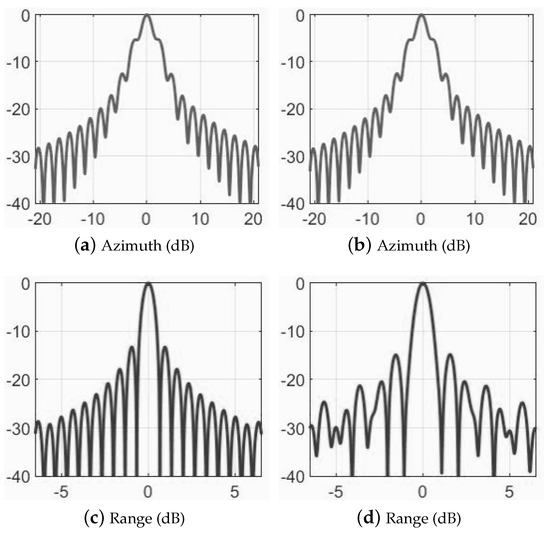
Figure 6.
Performance evaluation of point target in Figure 3: (a) azimuth section of point target by traditional method; (b) azimuth section of point target after reconstruction; (c) range section of point target by traditional method; (d) range section of point target after reconstruction.
Table 2.
Specific assessment details of Figure 6.
In Figure 7a,b, the average noise level is −93.81 dB by traditional method and −96.24 dB after reconstruction, resulting in a reduction of the noise level of 2.43 dB. However, the image exhibits peak power of 1.0018 and 0.6937 prior to and following reconstruction correspondingly, which means that there is some loss of energy. We looked into the causes of this loss in the later chapters.
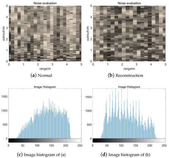
Figure 7.
Performance evaluation of regional noise: (a) ground noise of ship image by traditional method; (b) ground noise of ship image after reconstruction; (c) Image histogram of ground noise by traditional method; (d) Image histogram of ground noise after reconstruction.
To conclude, the signal-to-noise ratio has been augmented by 2.1219 dB. The peak side lobe ratio (PSLR) is also enhanced in terms of performance. As can be seen from Table 3, reconstruction weakens the background noise of the region, increases the equivalent viewing number and decreases the image contrast.
Table 3.
Results of regional noise evaluation.
In summary, the evaluation results verify the feasibility of the algorithm, the signal can be intactly recovered under the conditions of our corresponding experimental parameters, and the signal-to-noise ratio of the image has been improved to a certain extent. However, the evaluation results also give two new problems: one is the range ambiguity, and the other is the change of regional scene contrast. In order to explore the causes of these phenomena, we present our hypotheses and conduct further tests.
4. Error Analysis
4.1. Ambiguity Analysis of Reconstruction
According to the formula derivation logic in Section 2, the algorithm is applied in the echo domain; that is, the imaging process is as follows:
- 1.
- Sampling according to the code scheme;
- 2.
- Calculating the reconstruction matrix by the code to reconstruct the echo;
- 3.
- Imaging with the reconstructed echo.
Because of the SAR stop-go-stop hypothesis, the theoretical underpinnings of our method to reconstruct echo is that the echo received remains unchanged when the pulse waveform of the transmitter is identical. Nevertheless, even the distinct subpulses within the code correspond to different subapertures. The Doppler phase’s natural divergence can be negligible in the reconstruction solely when its disparity among all subpulses within the code is sufficiently minimal.
According to the above inference, we conclude that when observing a large range of scenes, the reconstruction algorithm will not work properly, because the reconstruction error changes with the Doppler phase and reaches its maximum at the edge of the aperture, which certainly leads to the deterioration of the performance of synthetic aperture. The mathematical logic can be interpreted as follows: the solution fuzzy equation constructed by the reconstruction matrix is underdetermined and has no solution, so we can only try to fit the data. We tested the imaging performance of large scenes to verify this idea, and the results are shown in Figure 8. A more aggressive coding was adopted here.
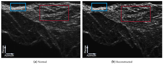
Figure 8.
Mountain scenes. The blue box shows the contrast enhancement. The red box shows the azimuth ambiguity.
Observe a mountain scene (N: 22486.50 E: 113573.42), and its evaluation results are shown in Figure 9. It can be seen that azimuth ambiguity (a,b) and region contrast changes (e,f) appear in the reconstructed image. Their edge detection results are shown in Figure 9c,d,g,h.
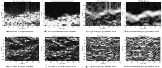
Figure 9.
Evaluation of large scenes.
In order to analyze the enhancement effect of reconstructed edge contrast and show the ambiguity in azimuth direction, we perform the ratio of average (ROA) edge detector (Chen et al., 2012, Touzi et al., 1988) on two regions marked by the red and blue box in Figure 8a,b [32,33]. In the edge detection processing, the 5 × 5 pixels local window is selected for detecting all potential edges [34].
It is easy to see from the edge detection results that the reconstruction algorithm takes effect normally in the range direction, which makes the target enhanced and the noise suppressed. However, in the azimuth direction, pixels are blurred and misaligned along the azimuth direction, resulting in a decrease in azimuth resolution.
Through the observation of the echo’s noise power, it becomes evident that there is a noticeable spatial variation effect in addition to the azimuth time, as depicted in Figure 10. As the distance from the synthetic aperture center increases, so does the disparity between the constructed matrix and the designed matrix, resulting in a larger fitting error [35,36]. The pulse code aligns most closely with the designed code only when the Doppler frequency reaches 0, enabling the echo to achieve the intended signal-to-noise ratio. However, in our reconstruction operation, all subaperture echoes are integrated so that azimuth leakage will directly lead to the reduction of the SNR [37,38].
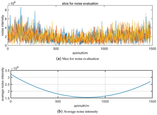
Figure 10.
Consider the effect of averaged power of noise changing with the azimuth variation.
4.2. Transmit–Receive Conversion Time
The transmit–receive conversion time is the time required for a hardware system to switch between the transmit and receive states. To simplify the analysis, it is assumed that the transmit–receive conversion time and the transmit–receive conversion time are equal. When there is a conversion time, in order to ensure that the signal is fully transmitted, the opening time of the receiving window should be delayed, and the closing time should be advanced. The result is a reduction in the duration of the entire receiving window. Suppose transmit–receive total time for , receiving window length , L is equivalent pulse width in a . M is the number of subpulses emitted in a . Since each transmitted pulse corresponds to a receiving window, the total echo reduction time is . Since the recovered echoes are linear combinations of original echoes from different receiving windows, the assumed coefficients are , the echoes of windows, such as , are affected by the sending and receiving conversion window. This will cause to be inconsistent with the ideal reconstructed echo, but it is limited to echoes before and after the reconstruction. After the reconstruction, the echoes of two adjacent subpulses are discontinuous, which will affect the final imaging results to a certain extent.
Simulate a signal and recover it. The main observation is whether the echo recovery is affected and how the noise ratio is affected. Suppose the code is 100000010010000 and each subpulse is 10 microseconds wide. Then, the transmitting window is the 1, 8, and 11 subpulse positions, and other windows are receiving windows. The simulation set a 500 nanosecond transceiver conversion time, as shown in Figure 11.
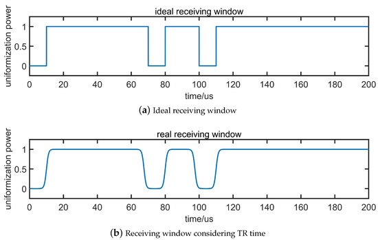
Figure 11.
Nanoseconds transmit–receive conversion time of 500 s.
The amplitude and phase of the recovered echoes were compared with or without the transceiver conversion. Due to the existence of transmit–receive conversion time, the power of the recovered echo appears to decrease in some moments, but the phase does not change. Pulse compression is performed on the echoes in both cases, and the comparison figure is shown in Figure 12. It can be seen that the gain of pulse compression results is reduced by about 0.16 dB due to the existence of transmit–receive conversion time.
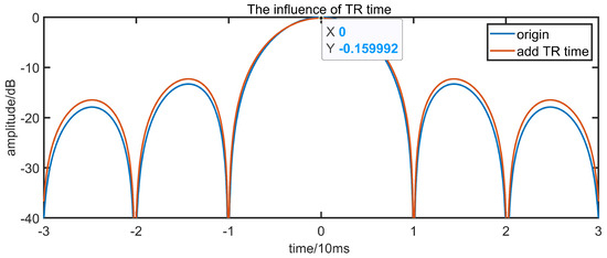
Figure 12.
Comparison of pulse compression results in two cases.
Then, the experiment was repeated by changing the target distance from 1.05 to 7.95 . Experimental results show that the gain of pulse pressure results in the worst case is reduced by about 0.4 dB. In summary, it is basically equivalent to the pulse compression energy loss caused by 5% energy loss of a single subpulse.
5. Coding Scheme Design
It has been basically proved that coding technology can improve the performance of images. It is a problem to consider that the corresponding coding under different wave positions can achieve the optimal effect.
First, once the length and subpulse width are fixed, augmenting the transmitting quantity results in a decrease in the receiving quantity, with the condition that the remaining time of the receiving window must not fall below the duration of the scene echo. Consequently, the encoding should aim for a more balanced distribution of the transmit and receive windows, meaning it should strive to guarantee that .
Second, by maintaining a constant total pulse width and decreasing the subpulse width, the decrease in SNR resulting from the decrease in subpulse width will nullify each other through echo reconstruction. Consequently, if the pulse width falls short of the upper duty cycle threshold, the impact of augmenting the subpulse width is equivalent to that of directly adding a new solitary subpulse.
Thirdly, once the pulse width attains the maximum threshold of the duty cycle, the attainment of SNR gain is unattainable through the division of the broad pulse into encoded pulse clusters that possess an identical overall pulse width. In addition, according to the previous analysis, the phase change will not change the final gain.
Therefore, after all the variables are normalized, for a code of a certain length, if the limit is only the difference of pulse emission position, without considering the phase difference between the emitter pulses, the number of codes is limited. So, the idea is to iterate over all codes while iterating the length of the code.
The beam positions of the system provided by the China Astronautic Sci-Tec Group LTD. 704 Research Institute are shown in Table 4.
Table 4.
Beam position design.
The scheme we adopt is as follows:
- (1)
- Calculate by beam position design.
- (2)
- Determine the echo window width under the constraint of design and obtain a sum of the maximum subpulse widths in .
- (3)
- Determine an encoding length L and divide equally into L parts.
- (4)
- If there are M subpulses in total, the length of the receiving window is .
- (5)
- Evaluate the resulting construction matrix to see if it is full rank.
- (6)
- Verify the recovery effects of our coding and evaluate its performance.
With the SNR increased by 2 dB and no obvious reconstruction error as the screening criteria, the coding schemes that meet the conditions are screened. The corresponding optimum design of these seven groups of beam positions is shown in Table 5.
Table 5.
Coding scheme design.
The gain and ambiguity results of the optimal coding scheme corresponding to the seven groups of beam position are shown in Table 6.
Table 6.
A detailed table of the position of the echo window to be recovered and its corresponding gain.
6. Conclusions
First of all, we give a robust coding design method, and successfully realize the echo reconstruction under spaceborne SAR conditions, and give the idea of reconstructing by part of the echo to reduce the amount of data calculation. Secondly, the simulation results show that our method can achieve the correct reconstruction of echoes and achieve an average 2.2 dB signal-to-noise ratio improvement. The simulation results show that due to the influence of Doppler effects, the reconstruction error changes obviously with the azimuth direction, resulting in a slight decrease in image power. Finally, we consider the impact of transmit–receive conversion time and perform a complete process analysis at the system level. The analysis results show that the effect of transmit–receive conversion time is equivalent to receiving window loss, and the specific SNR gain and error are related to wave position, coding and other parameters, which can be calculated accordingly.
The utilization of quasi-continuous-waveform coding technology offers a novel approach to designing spaceborne SAR systems. Different from multi-channel stagger SAR and other variable-PRF techniques, we use periodic coding. Different from other quasi-continuous-wave systems, we use the same linear frequency-modulated wave normalized in the time domain. These presettings allow us to explore the coding itself in more detail, but do not imply that our approach is mutually exclusive with the other techniques described above. Next, we will try more integration solutions.
We discuss in detail why the reconstruction error occurs in a long integration time. We give several schemes for weakening error, but for how to design the relevant weakening error schemes, we adopt the method of exhaustion, and fail to give the mathematical interpretable derivation and radical solution.
Unfortunately, we have not yet tried to apply this technique in multi-channel SAR due to equipment limitations. Therefore, it is one of our future research directions to introduce phase modulation in multi-channel SAR to solve the aliasing and ambiguity of single channels. The waveform design feature of the quasi-continuous-wave is mainly to maximize the average power of the radar transmitter, so the quasi-continuous-wave shape is more suitable for the application of long-range pulse measurement radar. It is expected that the coding technology of the quasi-continuous-wave system will have further application in spaceborne SAR in the future.
Author Contributions
Conceptualization, W.S.; methodology, T.L.; software, W.S.; validation, W.S.; formal analysis, W.S.; data curation, W.S.; writing—original draft preparation, W.S.; writing—review and editing, Q.W., P.S. and H.H.; visualization, W.S.; project administration, H.H.; funding acquisition, H.H. All authors have read and agreed to the published version of the manuscript.
Funding
This work is supported by the National Natural Science Foundation of China (grant no. 62071499), the introduced innovative R&D team project of “The Pearl River Talent Recruitment Program” (2019ZT08X751), the Key Areas of R&D Projects in Guangdong Province (grant no. 2019B111101001), and the Shanghai Academy of Spaceflight Technology (SAST2018-089).
Data Availability Statement
The data are not publicly available. Due to the adoption of a new system of radar we built ourselves, we collect and test our own data and do not use any open-source data. The relevant research is not complete, so we will not publish these data at this time.
Acknowledgments
Special thanks to Li Li for his long-term guidance of this work. Thanks to Han YaQuan for his proofreading of this article.
Conflicts of Interest
The funders had no role in the design of the study; in the collection, analyses, or interpretation of data; in the writing of the manuscript; or in the decision to publish the results.
Abbreviations
The following abbreviations are used in this manuscript:
| SAR | Synthetic aperture radar |
| SNR | Signal-to-noise ratio |
| HRWS | High-resolution wide swath |
| TR | Transmit–receive |
References
- Wang, Y.; Li, H.; Han, S. The theory and method of pulse coding for radar and its applications. J. Radars 2019, 8, 1–16. [Google Scholar]
- Wang, Y.; Liu, C.; Zhan, X.; Han, S. Technology and applications of UAV synthetic aperture radar system. J. Radars 2016, 5, 333–349. [Google Scholar]
- Khan, R.H.; Mitchel, D.K. Wave analysis for high frequency FMICW radar. IEEE Process.-F 1991, 138, 411–419. [Google Scholar]
- Yuan, S.; Chen, G.; Li, G. The digital signal processing system of quasi-continuous wave radar. J. Inst. Command. Technol. 2002, 13, 67–69. [Google Scholar]
- Zeng, T.; Long, T.; Wang, H. The design and realization of quasi-continuous tracking radar signal processor. J. Beijing Inst. Technol. 1999, 19, 604–606. [Google Scholar]
- Gao, B.; Ye, Z. The algorithm selection of maximum entropy spectral estimation based on quasi-continuous wave radar. Electron. Warf. Technol. 2003, 18, 26–31. [Google Scholar]
- Kovregin, V.N.; Kovregina, G.M.; Murzaev, A.S. Method for Detection/Identification of Several Air Objects with a Complex Spectrum in Radars with Quasi-Continuous Chirp Radiation. In Proceedings of the 2022 Wave Electronics and its Application in Information and Telecommunication Systems (WECONF), St. Petersburg, Russia, 30 May–3 June 2022; pp. 1–5. [Google Scholar]
- Kalenichenko, S.P.; Mettus, L.; Veremjev, I. The opportunity of applying a complex modulation laws radar signals for remote sensing low atmosphere and water surface by ground-based radar. In Proceedings of the Fifth International Conference on Remote Sensing of the Marine and Coastal Environments, San Diego, CA, USA, 5–7 October 1998; pp. 1–3. [Google Scholar]
- Barkhatov, A.V.; Kalenichenko, S.P.; Kutuzov, V.M. Multiband radar complex for remote monitoring of water areas. J. Min. Inst. 2001, 149, 244–247. [Google Scholar]
- Toutin, T. Impact of RADARSAT-2 SAR ultrafine-mode parameters on stereo-radargrammetric DEMs. IEEE Trans. Geosci. Remote Sens. 2010, 48, 3816–3823. [Google Scholar] [CrossRef]
- Mcgregor, J.A.; Poulter, E.M.; Smith, M.J. Switching system for single antenna operation of an S-band radar. IEEE Proc-Radar Sonar Navig. 1994, 1, 141–144. [Google Scholar] [CrossRef]
- Yuan, W. Study on the design method of quasi-CW radar waveform. In Proceedings of the CIE International Conference on Radar, Shanghai, China, 16–19 October 2006; pp. 1–4. [Google Scholar]
- Yuan, W. Study on the Design Method of a Novel Quasi-CW Radar Waveform. Morden Radar 2007, 29, 16–19. [Google Scholar]
- Su, F.; Gao, M.; Tian, L. Research on eclipse problem of quasi-CW phase-coded radar and solutions. Acta Armamentarii 2009, 30, 714–718. [Google Scholar]
- Wang, H.; Zhang, J.; Li, Y.; Zhu, X. Anti-range eclipse waveform optimization method for quasi-CW radar. J. Data Acquis. Process. 2011, 26, 531–535. [Google Scholar]
- Zeng, W.; Sun, Y.; Xu, H.; Pan, L. Waveform design and parameters calculation for quasi-continuous wave radar system. Syst. Eng. Electron. 2013, 35, 517–521. [Google Scholar]
- Gu, H.; Li, X.; Shang, W. A new approach of periodic square wave interruption to solution of the leakage of CW radar. Acta Electron. Sin. 1998, 26, 7–11. [Google Scholar]
- Peng, W.; Wang, X.; Zhao, J. Methods of eliminating Doppler dispersion in synthetic wideband signal. In Proceedings of the International Conference on Microwave and Millimeter Wave Technology, Nanjing, China, 21–24 April 2008; pp. 1540–1543. [Google Scholar]
- Li, B.; Zhou, S.; Stojanovie, M.; Freitag, L.; Willett, P. Multicarrier communication over underwater acoustic channels with nonuniform Doppler shifts. IEEE J. Ocean. Eng. 2008, 33, 198–209. [Google Scholar]
- Zeng, X.; Liu, X.; Bai, J.; Zhang, Y.S. Study of space borne SAR multidimensional waveform encoding technology based on azimuth multi-beams multi-phase centers. Acta Electron. Sin. 2013, 41, 1863–1868. [Google Scholar]
- Xu, W.; Deng, Y. Multi-channel SAR with reflector antenna for highresolution wide-swath imaging. IEEE Antennas Wirel. Propag. Lett. 2010, 9, 1123–1127. [Google Scholar] [CrossRef]
- Liang, D.; He, F.; Dong, Z. A Novel Space-Time Coding Alamouti Waveform Scheme for MIMO-SAR Implementation. IEEE Geosci. Remote Sens. Lett. 2015, 12, 229–233. [Google Scholar]
- He, F.; Zhang, Y.; Sun, Z.; Jin, G.; Dong, Z. Performance investigation on elevation cascaded digital beamforming for multidimensional waveform encoding SAR imaging. J. Radars 2020, 9, 828–855. [Google Scholar]
- Villano, M.; Krieger, G. Staggered SAR: High-Resolution Wide-Swath Imaging by Continuous PRI Variation. IEEE Trans. Geosci. Remote Sens. 2014, 52, 4462–4479. [Google Scholar] [CrossRef]
- Shao, W.; Huang, H. Study on Improving Imaging Quality of Spaceborne SAR by Pulse Coding Technology. In Proceedings of the International Academic Exchange Conference on Science and Technology Innovation, Chongqing, China, 8–9 December 2022; pp. 771–775. [Google Scholar]
- Bordoni, F.; Younis, M.; Krieger, G. Ambiguity Suppression by Azimuth Phase Coding in Multichannel SAR Systems. IEEE Trans. Geosci. Remote Sens. 2012, 50, 617–629. [Google Scholar] [CrossRef]
- Liu, J.; Xu, S.; Gao, X.; Li, X.; Zhuang, Z.W. A review of radar imaging technique based on compressed sensing. IEEE Signal Process. 2011, 27, 251–260. [Google Scholar]
- Basit, A.; Khan, W.; Khan, S.; Qureshi, I. Development of frequency diverse array radar technology: A review. IET Radar Sonar Navig. 2018, 12, 165–175. [Google Scholar] [CrossRef]
- Zhao, Q.; Zhang, Y.; Wang, W.; Deng, Y.; Yu, W.; Zhou, Y.; Wang, R. Echo separation for space-time waveform-encoding SAR with digital scalloped beamforming and adaptive multiple null-steering. IEEE Geosci. Remote Sens. Lett. 2020, 18, 92–96. [Google Scholar] [CrossRef]
- Zhao, Q.; Zhang, Y.; Wang, W.; Liu, K.; Deng, Y.; Zhang, H.; Wang, Y.; Zhou, Y.; Wang, R. On the frequency dispersion in DBF SAR and digital scalloped beamforming. IEEE Trans. Geosci. Remote Sens. 2020, 58, 3619–3632. [Google Scholar] [CrossRef]
- Ding, L.; Geng, F. Principle of Radar, 3rd ed.; Xidian University Press: Xi’an, China, 2002; pp. 1–22. [Google Scholar]
- Chen, S.; Wang, X.; Sato, M. PolInSAR complex coherence estimation based on covariance matrix similarity test. IEEE Trans. Geosci. Remote Sens. 2012, 50, 4699–4710. [Google Scholar] [CrossRef]
- Touzi, R.; Lopes, A.; Bousquet, P. A statistical and geometrical edge detector for SAR images. IEEE Trans. Geosci. Remote Sens. 1988, 26, 764–773. [Google Scholar] [CrossRef]
- Shen, P.; Wang, C. HoMeNL: A Homogeneity Measure-Based NonLocal Filtering Framework for Detail-Enhanced (Pol)(In)SAR Image Denoising. ISPRS J. Photogramm. Remote Sens. 2023, 197, 212–227. [Google Scholar] [CrossRef]
- Lan, L.; Liao, G. SAR Range Ambiguity Resolution Based on Element-Pulse-Coding. Radio Eng. 2021, 51, 675–680. [Google Scholar]
- Wang, C.; Xu, J.; Liao, G. A Range Ambiguity Resolution Approach for High-Resolution and Wide-Swath SAR Imaging Using Frequency Diverse Array. IEEE J. Sel. Top. Signal Process. 2017, 11, 336–346. [Google Scholar] [CrossRef]
- Li, Y.; Zhang, Y.; Liang, J.; Wang, Y. An Improved Omega-K Algorithm for Squinted SAR with Curved Trajectory. IEEE Geosci. Remote Sens. Lett. 2023, 21, 1–5. [Google Scholar] [CrossRef]
- Li, Y.; Huo, T.; Cao, C. An Efficient Imaging Method for Medium-Earth-Orbit Multichannel SAR-GMTI Systems. Remote Sens. 2022, 14, 5453. [Google Scholar] [CrossRef]
Disclaimer/Publisher’s Note: The statements, opinions and data contained in all publications are solely those of the individual author(s) and contributor(s) and not of MDPI and/or the editor(s). MDPI and/or the editor(s) disclaim responsibility for any injury to people or property resulting from any ideas, methods, instructions or products referred to in the content. |
© 2024 by the authors. Licensee MDPI, Basel, Switzerland. This article is an open access article distributed under the terms and conditions of the Creative Commons Attribution (CC BY) license (https://creativecommons.org/licenses/by/4.0/).