1. Text Correction
There was an error in the original publication [
1]. Thanks to valuable input from Dr. ZhongPing Lee, a typo was found in Charlotte Begouen Demeaux’s code computing
Kd(
λ)
Lee05. This resulted in the values of
Kd(
λ)
Lee05 used in the original paper being ≈12% lower than the corrected values. This difference was evenly spread across the range of
Kd(490)
Lee05 values; therefore, it does not affect the shape of the bias that was presented in this study. Therefore, the systematic overestimation of
Kd(490)
float by
Kd(
λ)
Lee05 is in the same range as the one by
Kd(490)
NN, and this happens for very low
Kd(490) values (<0.025 m
−1). Corrected values are presented in the paragraphs below. Please note that the changes have been marked in bold.
A correction has been made to Section 3.1 Kd(λ): Global Scale Match-Ups.
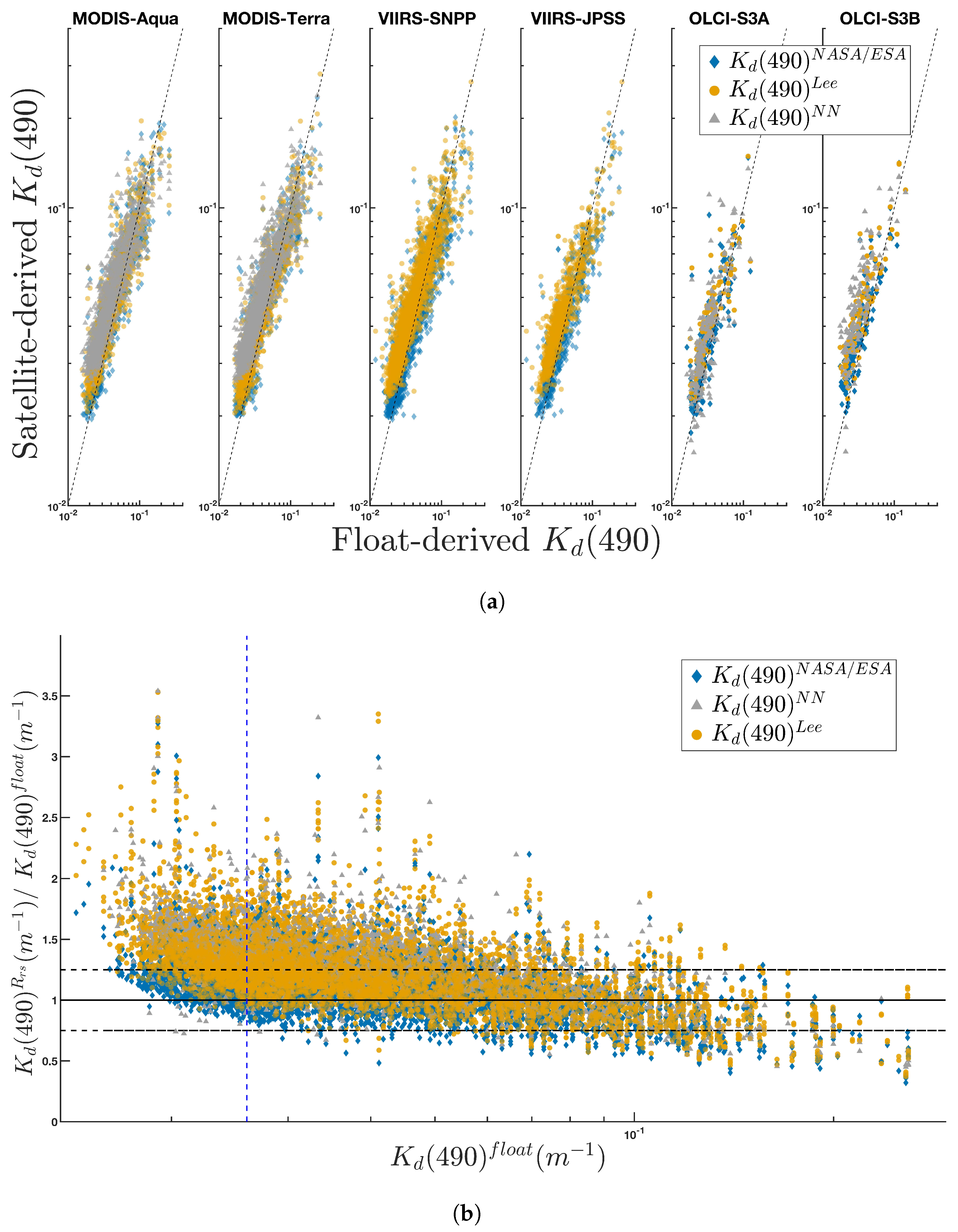
Kd(490)Rrs retrieved from each of the algorithms generally followed the 1:1 line (Figure 3). The operational products (Kd(490)NASA for MODIS and VIIRS, Kd(490)ESA for OLCI) had the best statistical results for the VIIRS and OLCI sensors, with the lowest Bias, APD and RMSE for each sensor (Table 3), and Kd(490)Lee05 had the best results for the MODIS sensors. Kd(490)NASA also retrieved the slope closest to one for all four sensors. Kd(490)Lee05 systematically overestimated Kd(490) at low Kd values (<0.025 m−1) and had a few outliers for the MODIS sensors (not plotted on Figure 3 but used in statistics) that impacted its r-score. Kd(490)NN had a slope furthest from one for the MODIS sensors and also showed a systematic overestimation at very low values (Kd(λ) < 0.025). The slopes were below one for all the sensors with a significant non-zero intercept. The Kd(490)Rrs/Kd(490)float ratio (Figure 3b) for low Kd values is larger for Kd values with a small zenith angle (≈10°), but for a given Kd value, a higher solar zenith angle resulted in a larger Kd(490)Rrs/Kd(490)float ratio.
The Kd(412)float range of values is 0.0126–0.7 m−1 (Figure 1 and Figure 4). The operational products are not computed at 412 nm and we therefore only compare KdLee05 and Kd(490)NN to Kd(490)float. Kd(412)NN performed significantly worse than Kd(412)Lee05 for the MODIS-Aqua, MODIS-Terra, and OLCI-S3B sensors, with a lower r-score and a higher bias, APD, and RMSD for all sensors (Table 4). For OLCI-S3A, Kd(412)NN performed better. The slopes are closer to one for each of the sensors than at λ = 490 nm while still showing a systematic overestimation for small Kd(412) < 0.026 values (Figure 3b), along with a significant non-zero intercept.
Both Kd(412)Lee05 and Kd(412)NN had a lower APD at 412 nm than at 490 nm for all three sensors; however, Kd(412)NN exhibited a larger RMSD. The slope is closer to one (all are >0.91). The ratio KdRrs/Kdfloat was closer to one at 412 nm than 490 nm (Figure 4).
A correction has been made to Section 3.2 Kd(PAR): Global Scales Matchups
The number of matchups between sensors-derived and floats-derived Kd(PAR) was 832 for MODIS-Aqua, 944 for MODIS-Terra, 1402 for VIIRS-SNPP, 613 for VIIRS-JPSS, 155 for OLCI-S3A and 227 for OLCI-S3B (Figure 5) resulting in a total of 4173 matchups between float and satellite. For all sensors, there was an underestimation for small values: Kd(PAR)float < 0.038 m−1 for Kd(PAR)Morel and Kd(PAR)float < 0.048 m−1 for Kd(PAR)Lee05 representing 11% and 20% of the full dataset, respectively. For those values, independent of the sensors, Kd(PAR)float < Kd(PAR)Rrs, with the ratio increasing as Kd(PAR)float decreased (Figure 5b). The regression slopes are <1 for both algorithms, and there was a significant intercept for both of them (Table 5).
Kd(PAR)Morel had a lower bias, lower APD, lower RMSD and a higher r than Kd(PAR)Lee05 (Table 5). It also had a slope closer to one. For high values, Kd(PAR)Lee05 > Kd(PAR)Morel, whereas for low values, Kd(PAR)Morel > Kd(PAR)Lee05 (Figure 5). The biggest discrepancy between the two algorithms occurs when the Solar zenith angle is low (<20°), but for a given Kd(PAR)float value, the higher the solar zenith angle, the bigger the difference.
A correction has been made to Section 3.3: Variability in Performance between Satellite Sensors (paragraph 1 and 3).
We performed a Kolmogorov–Smirnov (K-S) test to assess whether the distributions of KdRrs (λ) retrieved by a given sensor using different algorithms were different. The K-S test indicates whether the Kd values retrieved by different algorithms have a different distribution within a given confidence interval (here 5%). The distributions of Kd(490)NN vs. Kd(490)Lee05 retrieved by the OLCI-S3A sensor were not statistically different from each other (Table 3), whereas, they were different for the other sensors. The distribution of Kd(490)Lee05 vs. Kd(490)NASA/ESA was statistically different for all sensors as was the case for the distribution of Kd(490)NN.
For all three algorithms tested, the only ones that had a similar distribution were for the Kd(490)NASA/ESA algorithm of the VIIRS-SNPP/OLCI-S3B sensor pair, the Kd(490)Lee05 algorithm between the OLCI-S3B/VIIRS-SNPP and for the OLCI-S3B/VIIRS-JPSS pairs. All other sensor pairs had statistically different distributions.
A correction was made to paragraph 3 of Section 3.4: Regional Analysis.
No obvious biome-based bias in algorithm performance was observed (Table 6), with biome 9 having the lowest bias and RMSD across all three algorithms but having slopes significantly different from one. Similarly, biome 18 had slopes close to one for Kd(490)Lee05 and Kd(490)NN but lower r than other biomes, such as biome 19. Note that some biomes (e.g., 6, 8, 10, 12, and 14) had a low number of matchups and limited dynamic range resulting in (non-significant) negative slopes and r.
A correction was made to the numbers presented in Section 4.1: Observed Biases in Kd.
All four algorithms had a slope < 1 at λ = 490 (Table 3) because Kd(490)Rrs > Kd(490)float at small Kd values. This overestimation of Kd(490) effectively leads to an underestimation of the depth to which light penetrates in the water column, potentially resulting in an under-estimation of heat transfer to depth and other depth-derived products from Kd(490). On the other hand, for Kd(490) > 0.1, Kd(490)Rrs < Kd(490)float (Figure 3). This underestimation of Kd will result in the overestimation of Kd(490)-derived products. The overestimation at small values is also found at λ = 412, with a systematic overestimation for Kd(412)NN and Kd(412)Lee05 at values < 0.025 (Figure 4). However, there is no persistent underestimation for larger Kd(412) values (Table 4).
It is also relevant to note that there is a strong relationship between Kd(490)float and Rrs-retrieved Chl a (r-score of 0.84 over the full matchup dataset), which is only slightly lower than the correlation score between the full Kd(490) float and Kd(490)Lee05 (0.89 over the full dataset) which asks the question about redundancy between the offered Satellite L2 products.
A correction was made to the numbers presented in the third, fourth and sixth paragraph of Section 4.2: Limitation of Datasets Used to Train Empirical Algorithm
We found the slopes of the regression between algorithm and float to typically be significantly less than one. If the regression intercept is forced to zero, the slope of Kd(490)Rrs vs. Kd(490)float is closer to one, regardless of algorithm or sensors (Table A3). It ranges from [1.03−1.17] for Kd(490)Lee05, [1.15−1.30] for Kd(490)NN, and [0.98−1.14] for Kd(490)NASA/ESA. It is apparent that the small values that are not sufficiently represented in the original range drive the slope offset we found.
Overall for Kd(490)Lee05, 74% of the values were within ±25% of Kd(PAR)float, 49% for Kd(490)NN, and 80% for Kd(490)NASA/ESA (Figure 3b). Therefore, the performances of the algorithms were significantly lower than on the original datasets they were based on, indicating that they could be improved. At 412 nm, 64% of Kd(412)Lee05 were within ±25% of Kd(412)float versus 65% for Kd(412)NN.
Similarly, Kd(PAR)Morel and Kd(PAR)Lee05 were designed using available in situ databases (NOMAD, among others mentioned above) or the IOCCG dataset, resulting in similar biases to those observed for Kd(412) and Kd(490). Clear-water biases are more important than for Kd(λ): 53% of Kd(PAR)Lee05 values were within ±25% of Kd(PAR)float and 20% of were consistently overestimated (Kd(PAR)float < 0.048). Some 53% of the Kd(PAR)Morel were within ±25% of Kd(PAR)float, and 11% were systematically overestimated (Kd(PAR)float < 0.039). Note that the overestimation of Kd(PAR) was first pointed out by the authors of [2].
2. Error in Figures/Tables
Figure 3.
Comparison of satellite-derived and float-derived Kd(490) for the MODIS-Aqua, MODIS-Terra, VIIRS-JPSS, VIIRS-SNPP, OLCI-S3A and OLCI-S3B sensors: (a) (490) computed using the 3 different algorithms compared to (490); the black dashed line is the 1:1 line; (b) (490)/(490) for each of the 3 evaluated algorithms (color coded) for all sensors; the solid black line is a ratio of 1, and the dashed black lines are the 0.75 (Bottom) and 1.25 (Top) ratio. The vertical dashed blue line indicates the minimum value of Kd(490) present in the NOMAD dataset (0.026).
Figure 4.
Comparison of satellite-derived and float-derived Kd(412) for the two MODIS and the two OLCI sensors: (a) (412) computed using the 2 different algorithms compared to (412); the black dashed line is the 1:1 line. (b) / for the matchups; the solid black line is a ratio of 1, and the dashed black lines denote ratios of 0.75 (Bottom) and 1.25 (Top) ratio; the dashed blue line indicates the minimum value of Kd(411) present in the NOMAD dataset (0.026).
Figure 5.
Results of the comparison between the satellite-derived and the float-retrieved , for two different PAR algorithms: (a) vs. colored by solar zenith angle with each marker shape indicating a different sensor; the dashed line indicates the 1:1 line; vs. (left), vs. (center) vs. (right); (b) ratio for each of the two algorithms against ; the solid line is a ratio of 1 and the dashed black lines denote ratios of 0.75 and 1.25.
Table 3.
Comparison of performance statistics at the global scale of the Kd(490 nm) for the MODIS, VIIRS, and OLCI sensors at the global scale and Kd(490 nm) algorithms. See Methods section for the definitions of the metrics. All distributions within a given sensor are statistically different. N represents the number of matchups with data at 490 nm.
| Sensor & Algo | BIAS | APD (%) | RMSD (m−1) | r | Slope | Intercept | N |
|---|
| MODIS-Terra: KdLee05 | 1.08 | 18.62 | 0.01 | 0.90 | 0.78 | 0.010 | |
| MODIS-Terra: KdNN | 1.31 | 33.72 | 0.02 | 0.87 | 0.76 | 0.018 | 2144 |
| MODIS-Terra: KdNASA | 1.13 | 20.37 | 0.01 | 0.90 | 0.84 | 0.010 | |
| MODIS-Aqua: KdLee05 | 1.11 | 19.58 | 0.01 | 0.89 | 0.82 | 0.011 | |
| MODIS-Aqua: KdNN | 1.27 | 31.19 | 0.02 | 0.86 | 0.79 | 0.017 | 1802 |
| MODIS-Aqua: KdNASA | 1.12 | 19.67 | 0.01 | 0.89 | 0.89 | 0.009 | |
| VIIRS-SNPP: KdLee05 | 1.16 | 22.46 | 0.02 | 0.88 | 0.77 | 0.013 | 3290 |
| VIIRS-SNPP: KdNASA | 1.06 | 17.36 | 0.02 | 0.88 | 0.78 | 0.010 | |
| VIIRS-SNPP: KdLee05 | 1.16 | 22.46 | 0.02 | 0.88 | 0.77 | 0.013 | 2445 |
| VIIRS-SNPP: KdNASA | 1.06 | 17.36 | 0.02 | 0.88 | 0.78 | 0.010 | |
| OLCI-S3A: KdLee05 | 1.16 | 21.46 | 0.01 | 0.84 | 0.79 | 0.012 | 651 |
| OLCI-S3A: KdNN | 1.19 | 26.62 | 0.01 | 0.77 | 0.91 | 0.008 | |
| OLCI-S3A: KdESA | 1.08 | 17.85 | 0.01 | 0.83 | 0.82 | 0.008 | |
| OLCI-S3B: KdLee05 | 1.25 | 27.73 | 0.01 | 0.91 | 0.68 | 0.018 | |
| OLCI-S3B: KdNN | 1.42 | 43.24 | 0.02 | 0.85 | 0.84 | 0.019 | 382 |
| OLCI-S3B: KdESA | 1.18 | 20.88 | 0.01 | 0.92 | 0.71 | 0.013 | |
Table 4.
Comparison of performance statistics at the global scale of the (412 nm) for the MODIS and OLCI sensors at the global scale and (412 nm) algorithms. See Methods section for the definitions of the metrics.
Table 4.
Comparison of performance statistics at the global scale of the (412 nm) for the MODIS and OLCI sensors at the global scale and (412 nm) algorithms. See Methods section for the definitions of the metrics.
| Sensor & Algo | BIAS | APD (%) | RMSD | r | Slope | Intercept | N |
|---|
| MODIS-Terra: KdLee05 | 1.13 | 11.60 | 0.06 | 0.68 | 0.91 | 0.010 | 1633 |
| MODIS-Terra: KdNN | 1.19 | 19.49 | 0.03 | 0.87 | 1.01 | 0.018 |
| MODIS-Aqua: KdLee05 | 1.10 | 8.91 | 0.02 | 0.86 | 0.88 | 0.011 | 1384 |
| MODIS-Aqua: KdNN | 1.15 | 16.01 | 0.03 | 0.88 | 1.09 | 0.017 |
| OLCI-S3A: KdLee05 | 1.19 | 20.68 | 0.02 | 0.93 | 0.98 | 0.012 | 269 |
| OLCI-S3A: KdNN | 1.15 | 13.67 | 0.02 | 0.88 | 0.92 | 0.008 |
| OLCI-S3B: KdLee05 | 1.23 | 23.23 | 0.02 | 0.92 | 0.85 | 0.018 | 326 |
| OLCI -S3B: KdNN | 1.34 | 35.02 | 0.02 | 0.87 | 1.20 | 0.019 |
Table 5.
Summary statistics for all satellite sensors at the global scale for both PAR algorithms. See Methods section for definitions of statistical metrics.
Table 5.
Summary statistics for all satellite sensors at the global scale for both PAR algorithms. See Methods section for definitions of statistical metrics.
| | MODIS-Terra | MODIS-Aqua | VIIRS-SNPP | VIIRS-JPSS | OLCI-S3A | OLCI-S3B |
|---|
| | Lee05 | Morel07 | Lee05 | Morel07 | Lee05 | Morel07 | Lee05 | Morel07 | Lee05 | Morel07 | Lee05 | Morel07 |
|---|
| Bias | 1.24 | 1.20 | 1.28 | 1.23 | 1.28 | 1.26 | 1.28 | 1.24 | 1.21 | 1.17 | 1.25 | 1.28 |
| ADP | 23.88 | 21.05 | 28.72 | 26.34 | 30.89 | 29.81 | 28.74 | 28.07 | 20.77 | 15.97 | 33.73 | 33.31 |
| RMSD | 0.027 | 0.032 | 0.031 | 0.035 | 0.031 | 0.037 | 0.029 | 0.035 | 0.028 | 0.034 | 0.026 | 0.028 |
| r | 0.87 | 0.75 | 0.86 | 0.76 | 0.86 | 0.75 | 0.88 | 0.77 | 0.81 | 0.65 | 0.92 | 0.85 |
| Slope | 0.83 | 0.61 | 0.90 | 0.68 | 0.82 | 0.57 | 0.77 | 0.53 | 0.85 | 0.53 | 0.94 | 0.69 |
| Intercept | 0.029 | 0.044 | 0.028 | 0.044 | 0.035 | 0.053 | 0.036 | 0.053 | 0.024 | 0.045 | 0.025 | 0.042 |
Table 6.
Summary statistics at λ = 490 nm for each of the biomes defined in Table A2, with all sensors grouped together. The NASA empirical algorithm (see Methods section) was applied for the MODIS and the VIIRS sensors, whereas the ESA empirical algorithm was applied on the OLCI sensors. As they are both empirical algorithms, they were grouped together for the overall statistical analysis. In parentheses are the numbers of matchups between Kd(490)float and Kd (490)Rrs in each of the biomes for each algorithm. For the definition of the bias, APD, RMSD and r (Pearson’s correlation coefficient) see the Methods section.
| | Biome 4 (N = 113) | Biome 6 (N = 35) | Biome 7 (N = 239) | Biome 8 (N = 76) | Biome 9 (N = 435) |
|---|
| | Lee | Jamet | Austin | Lee | Jamet | Austin | Lee | Jamet | Austin | Lee | Jamet | Austin | Lee | Jamet | Austin |
|---|
| BIAS | 1.13 | 1.25 | 1.08 | 1.16 | 1.35 | 1.20 | 1.18 | 1.31 | 1.11 | 0.95 | 1.04 | 0.88 | 0.97 | 1.01 | 0.96 |
| ADP | 17.57 | 29.58 | 13.65 | 18.38 | 35.04 | 21.08 | 19.92 | 35.38 | 14.38 | 25.38 | 30.85 | 25.90 | 21.03 | 25.30 | 20.72 |
| RMSD | 0.01 | 0.01 | 0.01 | 0.01 | 0.02 | 0.01 | 0.01 | 0.01 | 0.01 | 0.02 | 0.03 | 0.02 | 0.03 | 0.03 | 0.03 |
| r | 0.55 | 0.52 | 0.75 | 0.54 | 0.90 | 0.66 | 0.90 | 0.87 | 0.89 | −0.05 | −0.32 | 0.00 | 0.85 | 0.77 | 0.84 |
| Slope | 0.51 | 0.34 | 0.57 | 0.41 | 0.87 | 0.43 | 0.77 | 0.74 | 0.86 | −0.31 | −0.50 | −0.18 | 0.60 | 0.45 | 0.57 |
| Intercept | 0.02 | 0.03 | 0.02 | 0.03 | 0.02 | 0.03 | 0.01 | 0.02 | 0.01 | 0.09 | 0.11 | 0.08 | 0.03 | 0.05 | 0.03 |
| | Biome 10 (N = 6) | Biome 11 (N = 225) | Biome 12 (N = 21) | Biome 13 (N = 308) | Biome 14 (N = 10) |
| | Lee | Jamet | Austin | Lee | Jamet | Austin | Lee | Jamet | Austin | Lee | Jamet | Austin | Lee | Jamet | Austin |
| BIAS | 1.14 | 1.31 | 1.11 | 1.13 | 1.27 | 1.03 | 1.07 | 1.12 | 1.05 | 1.17 | 1.42 | 1.07 | 1.06 | 1.25 | 0.99 |
| ADP | 22.21 | 43.08 | 15.02 | 19.21 | 32.40 | 14.55 | 15.77 | 17.32 | 11.97 | 19.35 | 40.94 | 13.39 | 7.71 | 23.60 | 11.31 |
| RMSD | 0.02 | 0.03 | 0.01 | 0.01 | 0.01 | 0.00 | 0.01 | 0.01 | 0.01 | 0.01 | 0.01 | 0.00 | 0.00 | 0.01 | 0.01 |
| r | 0.61 | −0.65 | 0.82 | 0.53 | 0.50 | 0.60 | 0.63 | 0.59 | 0.69 | 0.83 | 0.70 | 0.84 | 0.84 | 0.12 | 0.64 |
| Slope | 0.43 | −0.47 | 0.65 | 0.43 | 0.46 | 0.49 | 0.52 | 0.56 | 0.62 | 0.64 | 0.59 | 0.70 | 1.11 | 0.24 | 1.29 |
| Intercept | 0.04 | 0.12 | 0.03 | 0.02 | 0.02 | 0.01 | 0.02 | 0.02 | 0.01 | 0.01 | 0.02 | 0.01 | 0.00 | 0.04 | −0.01 |
| | Biome 15 (N = 246) | Biome 16 (N = 184) | Biome 18 (N = 1554) | Biome 19 (N = 1986) |
| | Lee | Jamet | Austin | Lee | Jamet | Austin | Lee | Jamet | Austin | Lee | Jamet | Austin |
| BIAS | 1.07 | 1.17 | 1.08 | 1.11 | 1.28 | 1.07 | 1.05 | 1.17 | 1.04 | 1.10 | 1.27 | 1.05 |
| ADP | 23.50 | 30.17 | 22.35 | 19.52 | 34.44 | 17.00 | 17.59 | 24.43 | 16.80 | 17.58 | 29.20 | 15.42 |
| RMSD | 0.03 | 0.03 | 0.03 | 0.01 | 0.02 | 0.01 | 0.01 | 0.02 | 0.01 | 0.01 | 0.01 | 0.01 |
| r | 0.57 | 0.52 | 0.57 | 0.85 | 0.88 | 0.85 | 0.85 | 0.82 | 0.85 | 0.92 | 0.89 | 0.90 |
| Slope | 0.49 | 0.49 | 0.52 | 0.69 | 0.87 | 0.73 | 0.73 | 0.73 | 0.78 | 0.74 | 0.80 | 0.73 |
| Intercept | 0.03 | 0.04 | 0.03 | 0.02 | 0.02 | 0.02 | 0.01 | 0.02 | 0.01 | 0.01 | 0.02 | 0.01 |


