Abstract
Natural gas pipelines represent a critical infrastructure for most countries and thus their safety is of paramount importance. To report potential risks along pipelines, several steps are taken such as manual inspection and helicopter flights; however, these solutions are expensive and the flights are environmentally unfriendly. Deep learning has demonstrated considerable potential in handling a number of tasks in recent years as models rely on huge datasets to learn a specific task. With the increasing number of satellites orbiting the Earth, remote sensing data have become widely available, thus paving the way for automated pipeline monitoring via deep learning. This can result in effective risk detection, thereby reducing monitoring costs while being more precise and accurate. A major hindrance here is the low resolution of images obtained from the satellites, which makes it difficult to detect smaller changes. To this end, we propose to use transformers trained with low-resolution images in a change detection setting to detect pipeline risks. We collect PlanetScope satellite imagery (3 m resolution) that captures certain risks associated with the pipelines and present how we collected the data. Furthermore, we compare various state-of-the-art models, among which ChangeFormer, a transformer architecture for change detection, achieves the best performance with a 70% F1 score. As part of our evaluation, we discuss the specific performance requirements in pipeline monitoring and show how the model’s predictions can be shifted accordingly during training.
1. Introduction
Natural gas plays a critical role in the infrastructure of Germany, as well as numerous other countries. As of 2023, natural gas accounted for a significant portion of Germany’s energy production, serving as a vital energy source for millions of households and powering industrial production. Given its importance, it is imperative for pipeline operators to actively monitor their pipeline networks to ensure their operational integrity, enhance safety, and mitigate potential risks.
Various monitoring tools are employed to track essential parameters such as pipeline pressure, flow rates, and temperature, enabling the detection of corrosion, leakages, and other irregularities [1,2]. Gas pipelines are typically buried beneath the surface, which also exposes them to potential risks from human interference. For instance, construction activities involving digging or the accumulation of soil and heavy loads nearby can potentially damage the pipelines. Therefore, it is essential to monitor such external influences. Additionally, by law, pipeline operators must be aware of possible hazardous conditions near the pipeline that may cause damage. In the future, this will also be important for hydrogen pipelines, which are currently being developed and have the same monitoring needs as gas pipelines [3].
Presently, the monitoring of potential pipeline incidents is reliant on the utilization of helicopters, which conduct monthly flights along the pipeline. During these flights, human observers are responsible for identifying and documenting any observable alterations. However, this approach has several drawbacks, including high costs, environmental concerns, and the limited frequency of flights. Moreover, the pilots’ estimations regarding the location of their findings lack precise GPS coordinates and are prone to human error. The considerable time gap between flights, coupled with the extended length of the pipeline, makes it challenging to accurately recall the pipeline’s appearance from the previous month. Consequently, some potential incidents may go unnoticed.
In recent years, access to remote sensing data has become easier. More providers have entered the market, and the number of satellites orbiting Earth keeps growing. Satellite imagery has become increasingly more cost-effective, and the temporal resolution has increased. When a satellite passes over an area of interest, it acquires an image that can be monitored, with the exception of adverse weather conditions, which may impact the availability of new images. The growing amount of available data paves the way for the use of deep learning techniques for automated pipeline monitoring. This automated approach reduces the financial burden of helicopter flights and mitigates the need for substantial human involvement, thereby reducing potential errors and environmental impact. Furthermore, the regular updates provided by remote sensing imagery enable accurate tracking of changes over time. For example, during the construction phase, it becomes feasible to report various stages of building development or effectively monitor field growth and harvest cycles.
Change detection (CD) is a common task in remote sensing, where a model has to learn to detect relevant changes, given a pair of co-registered images. CD finds applications in diverse domains, including flood detection [4], monitoring glacier development [5], and urban changes [6]. Over the last decades, various models have been employed for CD [7] among which are convolutional neural networks. Recent advancements have shown promising outcomes with deep learning models based on the transformer architecture [8], particularly for high-resolution data (0.5 m) [9,10]. It is apparent that with higher image resolution, it is easier to detect changes. Unfortunately, with current satellite constellations, acquiring high-resolution data remains expensive, and updates are less often available than low-resolution data (3 m), making it less attractive for commercial use. (We use high-resolution for 0.5 m and low-resolution for 3 m imagery. In the literature, these definitions vary and change over time as the resolution increases with better sensors).
We propose to formulate the problem of pipeline monitoring as a CD task and present how ChangeFormer [9], a state-of-the-art transformer-based architecture for CD, can detect pipeline risks effectively. We collect a pipeline risk dataset using 3 m resolution PlanetScope satellite imagery, showing that transformer-based architectures can achieve good results even when working with low-resolution data. We also illustrate how ChangeFormer predicts risks and how its predictions can be tailored to meet the requirements of automated pipeline monitoring by adjusting for costs.
We begin by presenting how we collected our dataset and explain which changes are relevant for pipeline risk detection (Section 2). Next, we introduce the detection model (Section 3), provide quantitative and qualitative evaluations, and compare the model against other deep learning architectures (Section 4). Before concluding, we touch upon the related work (Section 5).
2. Risks of Natural Gas Pipelines
Our dataset comprises image pairs from the PlanetScope API, taken at different timesteps from the same location and their corresponding ground truth (GT) annotations. Figure 1 shows a sample from this dataset. In Germany, there are 540,000 km of pipelines providing households and factories with energy [11]. Typically, pipelines are located beneath the ground, although they may also be above ground or underwater. To collect the dataset, we initially determined the targeted coverage areas, focusing on mainland pipelines in Germany, where the external influence of human activities is the greatest.
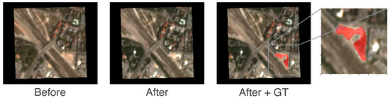
Figure 1.
A new construction site: Shown are satellite images before and after a new construction started. The task is to produce a binary map indicating the change, i.e., the ground truth (GT), which is shown here as a red overlay over the after image.
We proceeded to identify the relevant types of changes for pipeline monitoring. As a starting point, we had access to the reports from helicopter flights used previously to monitor the pipelines. Construction sites comprised the majority of the changes observed, with various agricultural changes, such as farmers piling up the harvest, following closely. Drawing from these helicopter reports, we compiled a comprehensive list of all previously observed changes. Additionally, we acknowledge the existence of other changes a human can detect that are not on the list. For these, we rely on human expertise to decide if they can pose a risk.
Using this list, we searched for changes seen at varying resolutions including on high-resolution (0.5 m) images. Pipelines in cities often branch to connect households, while larger direct pipelines link different cities. Our dataset includes rural and urban areas, so a model can learn to capture changes in both. To achieve this, we randomly selected patches from central and southern Europe, focusing on Germany, covering various landscapes and changes. We used Google Earth (we utilized Google Earth Pro for desktop (earth.google.com)) and its timestep function to locate the changes. For each identified change on Google Earth, we recorded the time of its first appearance and obtained two images at the same location from the PlanetScope API, with a resolution of 3 m. The first image (before image) does not include the change, while the second one (after image) does. A human annotator created a binary change mask for each change as the GT. We gathered 1372 before and after pairs and their binary masks and randomly split them into 80% for training, 10% for validation, and 10% for testing.
Collecting data for pipeline monitoring poses a challenging task since precisely specifying relevant changes is non-trivial. For instance, variations in sun exposure may lead to visible changes caused by reflected light from buildings or cars, which are no risk to the pipeline. Additionally, sensor degradation and other effects can subtly alter the pixel values of the spectral images [12], which should not impact the model’s predictions.
Defining the exact start of construction sites presents another challenge, as construction typically involves multiple stages such as vegetation or existing building removal, construction progress, and ultimately, the completion of the roof. Consequently, human annotators must determine when observed changes are noteworthy, leading to noisy labeling based on human judgment.
Another challenge is that small objects might not be visible on 3 m resolution images. For example, in the helicopter reports, there was a fallen perch next to a pipeline. Even for humans, detecting such a change on a 3 m resolution will be extremely challenging. Looking at higher-resolution images to find changes and then finding them at a lower resolution helped us cover smaller changes in the dataset. In general, though, the bigger the change, the higher its risk potential; therefore, we assume that all noteworthy changes can be seen with a 3 m resolution.
Finally, the PlanetScope API offers 8-band multispectral images dating back to 2020, which aligns with the time interval covered by our dataset [13]. However, we leave the utilization of 8-band data for future work. It is important to note that the dataset and helicopter flight reports are proprietary and thus cannot be made public. After establishing the data-gathering process, we next introduce the ChangeFormer model for CD.
3. Change Detection with Transformers
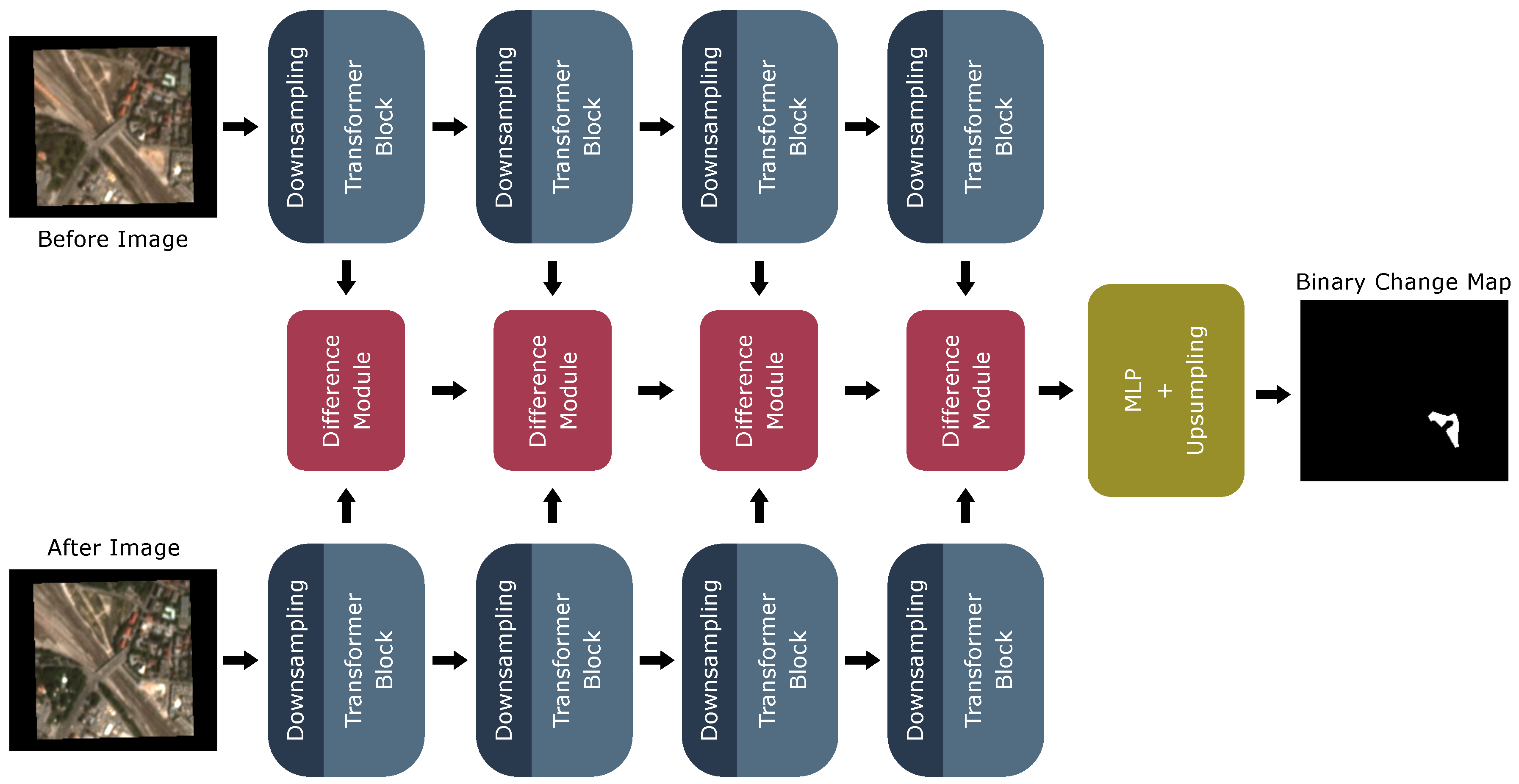
In CD, a model takes as input two co-registered images and produces a binary map indicating the change. During training, the model has to learn to differentiate between relevant changes, e.g., constructions, and non-relevant changes, e.g., seasonal changes or reflections. In this work, we use a state-of-the-art deep-learning-based CD model, ChangeFormer [9], shown in Figure 2. This section aims to give insights into the intermediate representations of ChangeFormer and how its attention mechanism is used for CD. For a more in-depth explanation of the computations carried out by each module, we refer to the original work of [9]. ChangeFormer consists of three stages:
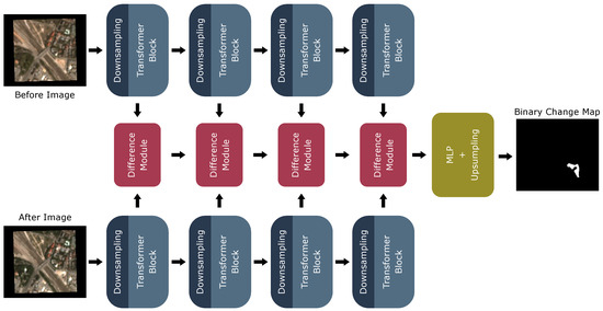
Figure 2.
The ChangeFormer model adapted from [9]: Four transformer modules produce features on different scales for the input images. The features from both images serve as input to the difference modules. These modules produce comparison features, which are forwarded through a multilayer perceptron (MLP) and upsampling module to output the binary change map.
- Feature extraction via four downsampling and transformer blocks (blue);
- Feature comparison using four difference modules (red);
- A decoder stage with a multilayer perceptron (MLP) and upsampling (yellow).
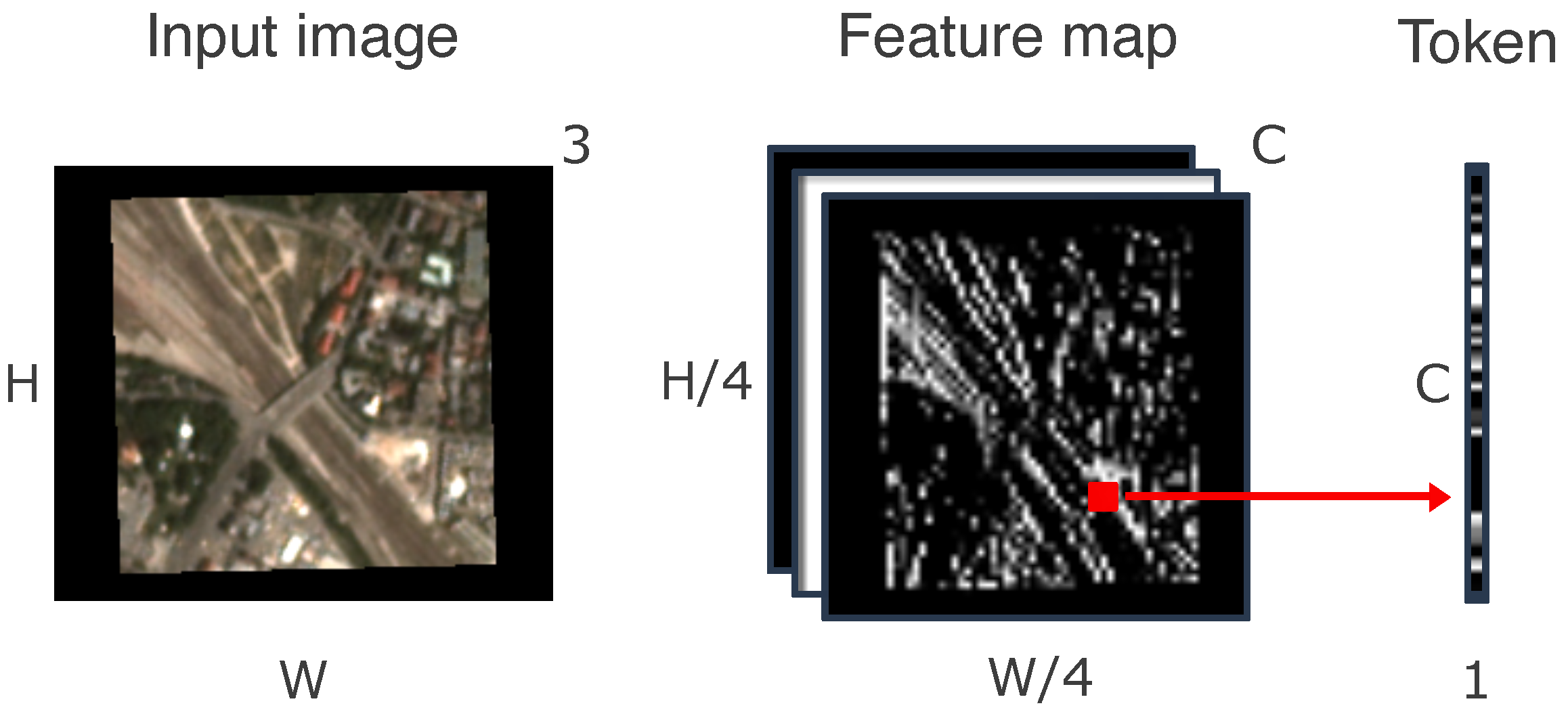
Originally, transformer models were introduced for natural language processing tasks [14] but have been adapted to work with images (cf. vision transformer [15]) and perform equally as well on visual tasks as architectures based on convolutional neural networks (CNNs). Transformers take as input a sequence of tokens. In the computer vision context, images are split into patches, which serve as the transformer input tokens. Unlike in the vision transformer, ChangeFormer, features are extracted by convolutions that downsample and extract features from overlapping patches in the input image. Afterwards, a positional encoding is added to the feature maps using another CNN and MLP step. Figure 3 shows how these feature maps are used as tokens for the transformer blocks. Each pixel in the feature map corresponds to one token with length C, which corresponds to the feature dimension. Together, all tokens (i.e., pixels) make up the input sequence for one transformer block.

Figure 3.
Extracting tokens: In ChangeFormer, a convolutional neural network (CNN) produces C feature maps of size from the input image. A token corresponds to one pixel along the feature map dimension C (marked in red).
At the heart of every transformer is an attention mechanism applied in the transformer block. Attention mechanisms produce a vector that weighs up which parts of the input sequence are essential for solving the specific task. The ChangeFormer model uses the scaled self-attention mechanism from [8]:
In self-attention, every input token can look at features from the same sequence of input tokens. K, Q, and V are all linear transformations of the input sequence. Every token emits features to find changes via its key K. The query Q binds to these features, and together, can be seen as the affinity of every token with each other. By multiplying by the value V, we obtain the aggregation of all important tokens for every token. The tokens are then enriched with the attention features, which is repeated for three rounds of attention.
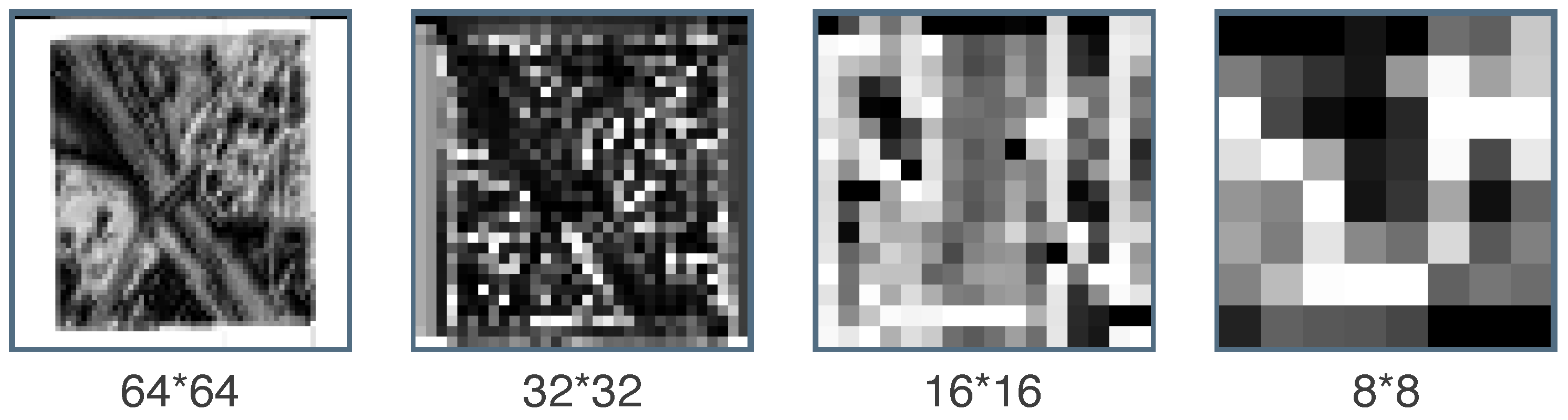
There are four transformer blocks that apply downsampling and the attention mechanism, and the attention-enriched feature maps from the previous block serve as the input for the next block. Intuitively, these attention-enriched feature maps contain features from each pixel and features from other pixels, which contain valuable information for the specific pixel. Furthermore, we can look for changes on different scales as all transformer blocks together extract hierarchical features on four different scales. Figure 4 shows attention maps on four scales after the first round of attention for the before image.
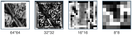
Figure 4.
Attention maps: ChangeFormer produces attention maps on different scales. Here, the mean attention map of all feature dimensions is shown after the first round of attention. The four scales correspond to the four transformer blocks shown in Figure 2. Areas containing houses are considered more on the 64 × 64 scale. On the lower scales, more high-level features are considered as the resolution decreases.
In the next step, each difference module compares concatenated features from both images with the same scaling. Consecutive difference modules also receive the output of previous difference modules. The difference module is a CNN that learns the differences during training. The last module is the decoder, which produces the binary change map shown on the right side of Figure 2. All features outputted by the difference modules on all scales are fed through an MLP and are upsampled. A softmax layer outputs the binary change map, including a change and non-change class. Note that the model can be easily extended to work with multiple change classes [16], e.g., vegetation and construction changes. Providing the model with semantic knowledge would certainly improve the performance and would be a fruitful direction for further research.
In our scenario, we use RGB remote sensing imagery. At the end of Section 1, we mentioned that hyperspectral data would be an interesting future research direction. The ChangeFormer architecture could be extended for hyperspectral data by changing the input channels and number of feature maps C to align with the hyperspectral bands. We argue that scaling the model to 12-band PlanetScope hyperspectral data should increase the memory footprint of the model as well as inference times but would likely be computationally feasible. In some cases, though, hyperspectral data come with considerably more bands, where these adjustments would not be feasible anymore, and other techniques are necessary. Lastly, empirical validation has to show whether such adjustments are sufficient and whether there will be a benefit of using them.
Trading precision for recall: In pipeline risk detection, our primary concern is capturing all relevant changes (recall) while keeping the number of false positives, also called false alarms, low (precision). It is hard to pinpoint what is more unacceptable: missing a change or predicting a non-existent one. A missed change could lead to severe power outages. On the other side, false positives must be checked on-site by the pipeline provider, which can also be costly. Weighing these against each other suggests that we do not want to miss a change but can tolerate some false positives. Moreover, a human in the loop can filter out false positives by comparing the model’s predicted change on the before and after images. Therefore, in this work, we prioritize higher recall and are willing to accept lower precision, although we would like to point out that models with a good balance between precision and recall are most desirable.
In [9], the loss function used to train ChangeFormer was the cross-entropy loss, which trades recall and precision equally. As argued, we can tolerate a lower precision if our recall is high enough. Thus, to shift predictive performance towards the recall, we can train ChangeFormer with the weighted cross-entropy defined as:
with weighting parameter , ground truth y, and prediction . The first part of the equation () is the entropy of the change class and the second part () is the entropy of the non-change class, both of which we want to minimize. During training, the weighting parameter shifts how much a missed change contributes relative to a false alarm towards the total loss. A value of one means an equal contribution. Selecting a value larger than one would lead to a bigger loss when a change is not detected, e.g., the model is trained more not to miss a change rather than to avoid false alarms. Vice versa, if we want to reduce the number of false alarms and are okay to miss some of the changes, we can pick a value smaller than one.
4. Experimental Evaluation
In this section, we demonstrate that ChangeFormer is a viable choice for detecting pipeline risks and compare it to other models. We first examine examples qualitatively and then perform a quantitative evaluation of our collected data. The aim of our experimental evaluation is to answer the following questions:
- Q1:
- Can ChangeFormer capture visual properties of relevant changes?
- Q2:
- How good is ChangeFormer at detecting relevant changes?
- Q3:
- Can we adjust for higher recall without significantly sacrificing precision?
We present the precision, recall, and F1 scores on a pixel- and object-based level to compare the models concerning the change class. Additionally, we report the Intersection over Union (IoU) at the pixel level to measure the prediction’s overlap with the GT. The mean and standard deviation are shown over five runs for every model. In the pixel-based metrics, the class of each pixel is checked. For the object-based metrics, we group pixel blobs by selecting all connected pixels of the change class, as they usually belong to a single change. A pixel blob is a true positive if it overlaps with any GT blob by more than four pixels; otherwise, it is a false positive. To avoid favoring models with many minor predictions, two prediction blobs overlapping the same GT blob are counted as one true positive. The object-based metric is helpful for pipeline monitoring since our primary focus is detecting wherever there was a change rather than precisely determining its exact boundaries.
Models: We test the vanilla ChangeFormer with randomly initialized weights. Additionally, we provide the results of ChangeFormer with pretrained weights from training on the LEVIR-CD dataset [17], which we call ChangeFormer-pt. LEVIR is a high-resolution CD dataset that focuses on building changes and is close to our setting. We use the weighted cross-entropy loss (Section 3) to allow for higher recall in exchange for precision. Different values for the weighting parameter (2, 4, 8) are considered to punish missed changes more than false alarms and we call these cost-adjusted variants ChangeFormer-ca. A value of 2 imposes twice the penalty for missed changes compared to a false alarm, whereas a value of 8 imposes an even more severe penalty for missed changes. As our baseline, we compare with other state-of-the-art transformer-based models and a CNN model, which was the best-performing CNN on the LEVIR dataset in [9].
- FC-Siam-conc [18] is a CNN-based Siamese network. It consists of an encoder producing features for both input images and a decoder that takes the concatenation of features on different scales as input to produce the output binary map. In [18], the authors also proposed FC-Siam-diff, which uses the difference of features in the decoder. We could not produce any predictions using this model, so we did not include it in our comparison.
- Bitemporal Image Transformer (BIT) [10] relies on a transformer encoder and decoder to enrich tokens obtained from a CNN. The tokens are then projected back to pixel space, where their difference is computed via subtraction, and another CNN is used to produce the binary change map.
- DTCDSCN [6] combines a change detection module with two semantic segmentation modules, which are trained together. Image segmentations and the binary change mask are provided as labels during training. This addition helps the model to focus more on object-level features and improves the performance on the evaluated task of building change detection. Note that in this work, we only use the CD part of the network, which involves, similar to the other BIT and ChangeFormer, obtaining features via convolutional layers and enriching them via attention.
- TinyCD [19] is again a Siamese structure that uses the attention mechanism over features extracted from a CNN. The main difference is in its size. While the current state-of-the-art models have millions of parameters, such as ChangeFormer with over 41 million, TinyCD only has a fraction with 280k parameters and still can achieve good performance on benchmark CD datasets. For a thorough comparison, we refer to the TinyCD paper [19].
Training: All models are trained for 200 epochs, and we use the AdamW optimizer and, as mentioned before, the cross-entropy loss with different weightings for ChangeFormer. We use the default hyperparameters (batch size of 16, learning rate is 0.0001 with a linear decay to zero) from [9] as they produce the best results and apply the same data augmentation during training. The same applies to the baselines, where we use the default parameters, loss functions, and data augmentation. We select the best-performing model on the validation split and report its performance on the unseen test set.
Q1. Qualitative evaluation: Figure 5 shows examples of six satellite images from the collected dataset. We observe that the ChangeFormer predictions overlap well with the GT. When the GT comprises more complex shapes, the model loses some details but obtains the right overall form. In two cases, the model predicts small blobs not in the GT (red circles). In Figure 6, ChangeFormer is compared with the baselines on our running example from Figure 1. All models detect the changes here but make another false prediction, except DTCDSCN, which only predicts one object. Qualitatively, ChangeFormer, TinyCD, and DTCDSCN match the GT the best, while the FC-Siam-Conc model predicts a significant change that is not in the GT. These results indicate that ChangeFormer learns the correct features to predict relevant changes. In some cases, it lacks some details but obtains the right overall shape of the GT. Table 1 shows the pixel-based performance. Here, we can observe that ChangeFormer and TinyCD have the highest IoU, which aligns with our qualitative observations—almost every second predicted pixel overlaps with the GT. FC-Siam-Conc and the BIT perform worse with ~13% less IoU.
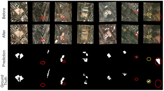
Figure 5.
Qualitative results: Shown from the top to bottom row are the before and after images, the prediction, and the GT from the ChangeFormer model [9]. The model can detect almost all changes represented in the GT, even in the case of three changes in one image, as in the fourth column. In some images, it predicts false positives (red circles). The last column again shows a false positive as it predicts the field being harvested as a change, but it also misses a small construction being started (yellow circle).
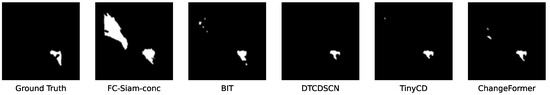
Figure 6.
Qualitative comparisons: In our running example (Figure 1), all models detect the construction site in the GT but miss its exact shape. Additionally, some models predict another change in the upper left corner that is not in the GT.

Table 1.
ChangeFormer variants achieve the best performance: On the pixel-based metrics, we can see that the ChangeFormer-pretrained (abbreviated pt) model achieves the highest F1 score and Intersection over Union (IoU). The FC-Siam-Conc model achieves comparable precision but has a lower recall. The BIT performs similarly to FC-Siam-Conc but favors the recall. Adjusting ChangeFormer for costs (abbreviated ca) can help us achieve higher recall while maintaining good precision. Color coding: best, 2nd-best, 3rd-best.
Q2. Model performance: On the pixel-based comparison in Table 1, we observe that TinyCD and ChangeFormer perform the best by a considerable margin compared with the BIT and FC-Siam-Conc baseline. The recall and precision of ChangeFormer are balanced. TinyCD has the best precision values and slightly worse recall values than ChangeFormer. FC-Siam-Conc achieves competitive precision values but has a lower recall, and DTCDSCN has slightly worse performance than the best-performing models.
Table 2 depicts the object-based performance. Here, DTCDSCN has the best F1 score followed by ChangeFormer. ChangeFormer detects approximately 80% of the changes, with a reasonably high precision exceeding 60%. Overall, most values are higher as this metric only considers wherever there was a change rather than how good predictions overlap with the GT. The considerable gap in recall between the metrics suggests that the models can locate changes well, but they occasionally do not perfectly overlap with the GT.
Table 2.
The cost-adjusted ChangeFormer strikes the right balance between precision and recall: The object-based metric provides us with a more accurate understanding of the number of changes we failed to capture. Again, ChangeFormer variants achieve ~80% and higher recall while having precision values of more than 49%. Adjusting for costs helps the transformer reach 88% recall. Color coding: best, 2nd-best, 3rd-best.
Comparing the standard deviation of the models, we see that most have a 1-2% standard deviation. The results of the FC-Siam-conc, BIT, and TinyCD baselines could be more consistent regarding their initialization, which favors ChangeFormer and DTCDSCN. High standard deviation values come from our dataset’s small number of samples and can be reduced by further data collection.
Pretraining ChangeFormer on the LEVIR-CD dataset [17] barely improves the F1 score on the pixel-based metric and even shows a slight decline in performance on the object-based evaluation. Generally, pretraining does not make much of a difference in this setting. We still argue that pretraining might be helpful in cases where little data are available, as in our study, or when a similar dataset can be used, preferably obtained from the same satellite.
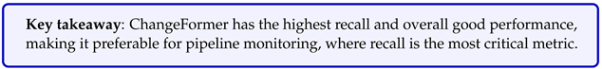
TinyCD and DTCDSCN perform the best on the pixel- and object-based metrics, respectively, followed by ChangeFormer, which places second on both metrics. Additionally, ChangeFormer has the best overall recall values, which is the most important metric for pipeline monitoring. Still, each of these three models would be suitable candidates as their performance differences are minor. In a deployment case in particular, the TinyCD model could be a good alternative to ChangeFormer due to its small model size, which could lead to savings in training the model.
Q3. Adjusting for higher recall: In Table 1 and Table 2, we observe that adjusting for higher recall yields positive results for both the pixel-based and object-based metrics and scales with higher values of . At the ×8 scaling, we can achieve above 88% recall on the object-based metric while maintaining reasonably high precision at approximately 50%. Initially, adjusting for costs benefits the F1 score and IoU, but with higher values, we notice a small negative effect. In summary, using the weighted cross-entropy loss is a simple but effective way to adjust the model to the performance requirements of pipeline monitoring.
5. Related Work
Change detection is an integral field in remote sensing with applications to various domains such as flood detection [4], glacier observation [5], and urban changes [6]. Given a pair of co-registered images, a model has to find the differences between them. What a change is depends on the specific task. As the taken images usually come with non-relevant changes, such as sensor degradation [12], a model has to learn which changes are of interest. Other works utilize a series of images to track changes over time rather than using a single pair of before and after images [20].
Over the last decades, the whole bandwidth of machine learning models has been used for CD in remote sensing [7]. In recent years, though, with the successes of deep learning, the focus has shifted towards these methods, and they have received much interest in the remote sensing community [21]. Various works focus on CD via deep learning [22], and CNNs especially are often applied for CD. With the rise of transformer architectures in natural language processing [8] and computer vision [15], these models have been deployed for remote-sensing tasks as well [23].
Transformers for CD: Multiple works [9,10,24,25,26] tackle CD with transformer-based architectures using some variation of the attention mechanism used in [8]. All of these works employ a Siamese-like structure that takes as input two images to produce a binary change map. Due to the successes of the vision transformer, there is an ongoing debate on whether to use CNNs or vision transformer-based methods for vision tasks [27]. In remote sensing, these principles are often seen in a combined way: The Bitemporal Image Transformer [10] uses a hybrid approach combining CNN features with the attention mechanism. ChangeFormer [9] employs a hierarchical transformer on different scales and learns a difference module. It applies the attention mechanisms to features extracted from a CNN. Works introducing transformer-based architectures have performed well on high-resolution data, while little work has been carried out on low-resolution data.
Pipeline monitoring is a broad field spanning many engineering disciplines. Many methods have been developed for monitoring the internal state of a pipeline [1,2] to detect abnormalities such as corrosion or leakages. To the best of our knowledge, methods for tracking external influences that can be harmful, such as construction sites next to a pipeline, are unexplored as of yet. The authors of [28] evaluate the potential use of technologies for construction site progress monitoring using remote sensing technologies. A related field is urbanization tracking, which is the closest to our setting [29].
Various CD datasets exist for urbanization tracking [17,30,31,32]. These datasets are benchmarks in various state-of-the-art CD models [9,10], and they all contain high-resolution images. One exception is the OSCD dataset covering low-resolution images with 10–60 m resolution [33]. Furthermore, the time interval varies among these datasets. Generally, there are longer intervals between the before and after images compared to our dataset, where time intervals are around one week. In the LEVIR-CD dataset [17], for example, many before images show undeveloped land, while the after images show finished settlements. In contrast, our dataset includes after images with recently started construction sites.
6. Conclusions
In conclusion, our exploration of the ChangeFormer architecture has showcased its great potential in risk detection through automated pipeline monitoring. With an evaluation conducted on a dataset encompassing pipeline risks, we illustrate that ChangeFormer exhibits impressive performance even with low-resolution images.
Among the many pipeline risks, construction sites and agricultural changes emerge as the most significant contributors. The cost-adjusted ChangeFormer accurately detected 88% of these risks, presenting a compelling alternative to previously utilized helicopter flights for monitoring purposes. The model’s capabilities could be further enhanced by incorporating hyperspectral data. Moreover, expanding the dataset to include a broader range of samples would empower the model to generalize better and handle a wider set of scenarios in the real world. Furthermore, formulating the task of CD over not just one pair of images but rather a series of images could be of great potential for more accurate monitoring. In addition, providing the model with diverse change classes would enable it to understand the semantics of the underlying changes more effectively and is a fruitful research direction.
Author Contributions
All authors were involved in the conceptualization, methodology, and validation of the project. Data curation: D.O., K.W., and S.B.; formal analysis, investigation, software and visualization: D.O.; writing—original draft preparation: D.O.; writing—review and editing: D.S.D., K.W., and K.K.; supervision: D.S.D. and K.K.; project administration: K.W. and S.B. All authors have read and agreed to the published version of the manuscript.
Funding
This work was partly supported by the ESA InCubed program “Automated satellite-based system for pipeline monitoring” (Project Nr. 4000134395/21/I-NS-bgh), the ICT-48 Network of AI Research Excellence Center “TAILOR” (EU Horizon 2020, GA No 952215), and the Collaboration Lab with Nexplore “AI in Construction” (AICO). It also benefited from the BMBF Competence Center KompAKI and the HMWK cluster project “The Third Wave of AI”.
Data Availability Statement
The dataset and helicopter flight reports are proprietary and, unfortunately, cannot be made public.
Conflicts of Interest
Authors Karsten Wiertz and Sebastian Bußmann were employed by the company SuperVision Earth. The remaining authors declare that the research was conducted in the absence of any commercial or financial relationships that could be construed as a potential conflict of interest.
Abbreviations
The following abbreviations are used in this manuscript:
| CD | change detection |
| GT | ground truth |
| CNN | convolutional neural network |
| MLP | multilayer perceptron |
| IoU | Intersection over Union |
| ca | cost-adjusted |
| pt | pretrained |
References
- Varela, F.; Tan, M.Y.; Forsyth, M. An overview of major methods for inspecting and monitoring external corrosion of on-shore transportation pipelines. Corros. Eng. Sci. Technol. 2015, 50, 226–235. [Google Scholar] [CrossRef]
- Adegboye, M.A.; Fung, W.K.; Karnik, A. Recent Advances in Pipeline Monitoring and Oil Leakage Detection Technologies: Principles and Approaches. Sensors 2019, 19, 2548. [Google Scholar] [CrossRef] [PubMed]
- Tsiklios, C.; Hermesmann, M.; Müller, T. Hydrogen transport in large-scale transmission pipeline networks: Thermodynamic and environmental assessment of repurposed and new pipeline configurations. Appl. Energy 2022, 327, 120097. [Google Scholar] [CrossRef]
- Longbotham, N.; Pacifici, F.; Glenn, T.; Zare, A.; Volpi, M.; Tuia, D.; Christophe, E.; Michel, J.; Inglada, J.; Chanussot, J.; et al. Multi-Modal Change Detection, Application to the Detection of Flooded Areas: Outcome of the 2009–2010 Data Fusion Contest. IEEE J. Sel. Top. Appl. Earth Obs. Remote Sens. 2012, 5, 331–342. [Google Scholar] [CrossRef]
- Xie, Z.; Haritashya, U.K.; Asari, V.K.; Young, B.W.; Bishop, M.P.; Kargel, J.S. GlacierNet: A deep-learning approach for debris-covered glacier mapping. IEEE Access 2020, 8, 83495–83510. [Google Scholar] [CrossRef]
- Liu, Y.; Pang, C.; Zhan, Z.; Zhang, X.; Yang, X. Building Change Detection for Remote Sensing Images Using a Dual-Task Constrained Deep Siamese Convolutional Network Model. IEEE Geosci. Remote Sens. Lett. 2021, 18, 811–815. [Google Scholar] [CrossRef]
- Asokan, A.; Anitha, J. Change detection techniques for remote sensing applications: A survey. Earth Sci. Inform. 2019, 12, 143–160. [Google Scholar] [CrossRef]
- Vaswani, A.; Shazeer, N.; Parmar, N.; Uszkoreit, J.; Jones, L.; Gomez, A.N.; Kaiser, L.; Polosukhin, I. Attention is All you Need. In Proceedings of the Annual Conference on Neural Information Processing Systems, Long Beach, CA, USA, 4–9 December 2017; Volume 30, pp. 5998–6008. [Google Scholar]
- Bandara, W.G.C.; Patel, V.M. A Transformer-Based Siamese Network for Change Detection. In Proceedings of the IEEE International Geoscience and Remote Sensing Symposium, Kuala Lumpur, Malaysia, 17–22 July 2022; pp. 207–210. [Google Scholar]
- Chen, H.; Qi, Z.; Shi, Z. Remote Sensing Image Change Detection With Transformers. IEEE Trans. Geosci. Remote Sens. 2022, 60, 1–14. [Google Scholar] [CrossRef]
- Deutscher Verein des Gas- und Wasserfaches. Available online: https://www.dvgw.de/themen/sicherheit/technische-sicherheit-gas (accessed on 20 July 2022).
- Wen, J.; Wu, X.; You, D.; Ma, X.; Ma, D.; Wang, J.; Xiao, Q. The main inherent uncertainty sources in trend estimation based on satellite remote sensing data. Theor. Appl. Climatol. 2023, 151, 915–934. [Google Scholar] [CrossRef]
- Tu, Y.H.; Johansen, K.; Aragon, B.; El Hajj, M.M.; McCabe, M.F. The radiometric accuracy of the 8-band multi-spectral surface reflectance from the planet SuperDove constellation. Int. J. Appl. Earth Obs. Geoinf. 2022, 114, 103035. [Google Scholar] [CrossRef]
- Wolf, T.; Debut, L.; Sanh, V.; Chaumond, J.; Delangue, C.; Moi, A.; Cistac, P.; Rault, T.; Louf, R.; Funtowicz, M.; et al. Transformers: State-of-the-art natural language processing. In Proceedings of the 2020 Conference on Empirical Methods in Natural Language Processing: System Demonstrations, Virtual, 16–20 November 2020; pp. 38–45. [Google Scholar]
- Dosovitskiy, A.; Beyer, L.; Kolesnikov, A.; Weissenborn, D.; Zhai, X.; Unterthiner, T.; Dehghani, M.; Minderer, M.; Heigold, G.; Gelly, S.; et al. An Image is Worth 16×16 Words: Transformers for Image Recognition at Scale. In Proceedings of the 9th International Conference on Learning Representations, Virtual, 3–7 May 2021. [Google Scholar]
- Toker, A.; Kondmann, L.; Weber, M.; Eisenberger, M.; Camero, A.; Hu, J.; Hoderlein, A.P.; Senaras, Ç.; Davis, T.; Cremers, D.; et al. DynamicEarthNet: Daily Multi-Spectral Satellite Dataset for Semantic Change Segmentation. In Proceedings of the Conference on Computer Vision and Pattern Recognition, New Orleans, LA, USA, 18–24 June 2022; pp. 21126–21135. [Google Scholar]
- Chen, H.; Shi, Z. A Spatial-Temporal Attention-Based Method and a New Dataset for Remote Sensing Image Change Detection. Remote Sens. 2020, 12, 1662. [Google Scholar] [CrossRef]
- Daudt, R.C.; Saux, B.L.; Boulch, A. Fully Convolutional Siamese Networks for Change Detection. In Proceedings of the IEEE International Conference on Image Processing, Athens, Greece, 7–10 October 2018; pp. 4063–4067. [Google Scholar]
- Codegoni, A.; Lombardi, G.; Ferrari, A. TINYCD: A (not so) deep learning model for change detection. Neural Comput. Appl. 2023, 35, 8471–8486. [Google Scholar] [CrossRef]
- Woodcock, C.E.; Loveland, T.R.; Herold, M.; Bauer, M.E. Transitioning from change detection to monitoring with remote sensing: A paradigm shift. Remote Sens. Environ. 2020, 238, 111558. [Google Scholar] [CrossRef]
- Ma, L.; Liu, Y.; Zhang, X.; Ye, Y.; Yin, G.; Johnson, B. Deep learning in remote sensing applications: A meta-analysis and review. ISPRS J. Photogramm. Remote Sens. 2019, 152, 166–177. [Google Scholar] [CrossRef]
- Khelifi, L.; Mignotte, M. Deep Learning for Change Detection in Remote Sensing Images: Comprehensive Review and Meta-Analysis. IEEE Access 2020, 8, 126385–126400. [Google Scholar] [CrossRef]
- Aleissaee, A.A.; Kumar, A.; Anwer, R.M.; Khan, S.; Cholakkal, H.; Xia, G.; Khan, F.S. Transformers in Remote Sensing: A Survey. Remote Sens. 2023, 15, 1860. [Google Scholar] [CrossRef]
- Guo, Q.; Zhang, J.; Zhu, S.; Zhong, C.; Zhang, Y. Deep Multiscale Siamese Network With Parallel Convolutional Structure and Self-Attention for Change Detection. IEEE Trans. Geosci. Remote Sens. 2022, 60, 1–12. [Google Scholar] [CrossRef]
- Zhang, C.; Wang, L.; Cheng, S.; Li, Y. SwinSUNet: Pure Transformer Network for Remote Sensing Image Change Detection. IEEE Trans. Geosci. Remote Sens. 2022, 60, 1–13. [Google Scholar] [CrossRef]
- Wang, G.; Li, B.; Zhang, T.; Zhang, S. A Network Combining a Transformer and a Convolutional Neural Network for Remote Sensing Image Change Detection. Remote Sens. 2022, 14, 2228. [Google Scholar] [CrossRef]
- Maurício, J.; Domingues, I.; Bernardino, J. Comparing Vision Transformers and Convolutional Neural Networks for Image Classification: A Literature Review. Appl. Sci. 2023, 13, 5521. [Google Scholar] [CrossRef]
- Moselhi, O.; Bardareh, H.; Zhu, Z. Automated Data Acquisition in Construction with Remote Sensing Technologies. Appl. Sci. 2020, 10, 2846. [Google Scholar] [CrossRef]
- Zhu, Z.; Zhou, Y.; Seto, K.C.; Stokes, E.C.; Deng, C.; Pickett, S.T.; Taubenböck, H. Understanding an urbanizing planet: Strategic directions for remote sensing. Remote Sens. Environ. 2019, 228, 164–182. [Google Scholar] [CrossRef]
- Liu, J.; Ji, S. A Novel Recurrent Encoder-Decoder Structure for Large-Scale Multi View Stereo Reconstruction From an Open Aerial Dataset. In Proceedings of the Conference on Computer Vision and Pattern Recognition, Seattle, WA, USA, 13–19 June 2020; pp. 6049–6058. [Google Scholar]
- Zhang, C.; Yue, P.; Tapete, D.; Jiang, L.; Shangguan, B.; Huang, L.; Liu, G. A deeply supervised image fusion network for change detection in high resolution bi-temporal remote sensing images. ISPRS J. Photogramm. Remote Sens. 2020, 166, 183–200. [Google Scholar] [CrossRef]
- Shi, Q.; Liu, M.; Li, S.; Liu, X.; Wang, F.; Zhang, L. A Deeply Supervised Attention Metric-Based Network and an Open Aerial Image Dataset for Remote Sensing Change Detection. IEEE Trans. Geosci. Remote Sens. 2022, 60, 1–16. [Google Scholar] [CrossRef]
- Daudt, R.C.; Saux, B.L.; Boulch, A.; Gousseau, Y. Urban Change Detection for Multispectral Earth Observation Using Convolutional Neural Networks. In Proceedings of the IEEE International Geoscience and Remote Sensing Symposium, Valencia, Spain, 22–27 July 2018; pp. 2115–2118. [Google Scholar]


Disclaimer/Publisher’s Note: The statements, opinions and data contained in all publications are solely those of the individual author(s) and contributor(s) and not of MDPI and/or the editor(s). MDPI and/or the editor(s) disclaim responsibility for any injury to people or property resulting from any ideas, methods, instructions or products referred to in the content. |
© 2024 by the authors. Licensee MDPI, Basel, Switzerland. This article is an open access article distributed under the terms and conditions of the Creative Commons Attribution (CC BY) license (https://creativecommons.org/licenses/by/4.0/).