Article

Cloud Overlap Features from Multi-Year Cloud Radar Observations at the SACOL Site and Comparison with Satellites

1
Key Laboratory for Semi-Arid Climate Change of the Ministry of Education and College of Atmospheric Sciences, Lanzhou University, Lanzhou 730000, China
2
Henan Key Laboratory of Agrometeorological Support and Applied Technique, CMA, Zhengzhou 450000, China
*
Author to whom correspondence should be addressed.
Remote Sens. 2024, 16(2), 218; https://doi.org/10.3390/rs16020218
Submission received: 30 October 2023 / Revised: 18 December 2023 / Accepted: 26 December 2023 / Published: 5 January 2024
(This article belongs to the Special Issue Remote Sensing of Aerosol, Cloud and Their Interactions)

Abstract

:
Cloud overlap, referring to distinct cloud layers occurring over the same location, is essential for accurately calculating the atmospheric radiation transfer in numerical models, which, in turn, enhances our ability to predict future climate change. In this study, we analyze multi-year cloud overlap properties observed from the Ka-band Zenith Radar (KAZR) at the Semi-Arid Climate and Environment Observatory of Lanzhou University’s (SACOL) site. We conduct a series of statistical analyses and determine the suitable temporal-spatial resolution of 1 h with a 360 m scale for data analysis. Our findings show that the cloud overlap parameter and total cloud fraction are maximized during winter-spring and minimized in summer-autumn, and the extreme value of decorrelation length usually lags one or two seasons. Additionally, we find the cloud overlap assumption has distinct effects on the cloud fraction bias for different cloud types. The random overlap leads to the minimum bias of the cloud fraction for Low-Middle-High (LMH), Low-Middle (LM), and Middle-High (MH) clouds, while the maximum overlap is for Low (L), Middle (M), and High (H) clouds. We also incorporate observations from satellite-based active sensors, including CloudSat, Cloud-Aerosol Lidar, and Infrared Pathfinder Satellite Observations (CALIPSO), to refine our study area and specific cases by considering the total cloud fraction and sample size from different datasets. Our analysis reveals that the representativeness of random overlap strengthens and then weakens with increasing layer separations. The decorrelation length varies with the KAZR, CloudSat-CALIPSO, CloudSat, and CALIPSO datasets, measuring 1.43 km, 2.18 km, 2.58 km, and 1.11 km, respectively. For H, MH, and LMH clouds, the average cloud overlap parameter from CloudSat-CALIPSO aligns closely with KAZR. For L, M, and LM clouds, when the level separation of cloud layer pairs are less than 1 km, the representative assumption obtained from different datasets are maximum overlap.

1. Introduction

Clouds are composed of liquid water droplets, ice crystals, or a combination of both suspended in the atmosphere. Clouds reflect incoming solar radiation back into space, resulting in a cooling effect known as the albedo effect. Meanwhile, they absorb and trap outgoing longwave radiation from the Earth, leading to a warming effect recognized as the greenhouse effect [1,2,3,4]. Clouds are also intricately linked to the water vapor cycle in the atmosphere. As global temperatures rise, the atmosphere is expected to hold more water vapor that will condense to form clouds under specific meteorological conditions. These shifts can either amplify or mitigate the initial warming or cooling effects of clouds due to changes in their properties, known as cloud feedback.
Clouds’ radiative effects are highly dependent on the horizontal and vertical distribution of cloud layers. In the natural environment conducive to cloud formation, clouds often manifest as distinct layers occurring at various altitudes over the same location within the vertical column of the atmosphere. This refers to cloud overlap that determines the vertical dispersal of cloud property and strongly affects the radiation entering and exiting the atmosphere, leading to quite different radiative heating rates and consequently different temperature responses to changes in greenhouse gas concentrations [5,6]. Therefore, variations in cloud overlap hold the potential to significantly influence Earth’s radiative energy balance, atmospheric circulation and precipitation pattern, and the efficiency of cloud feedback mechanisms in either amplifying or dampening global warming.
Cloud formation and development involve complex physical and dynamic processes, leading to dramatic temporal and spatial variability and presenting challenges in accounting for the coexistence of different cloud types [7,8]. In general, two cloud layers at different altitudes can exhibit varying degrees of separation, ranging from horizontal separation (non-overlapping) to vertical stacking, where one layer sits atop the other (overlapping). Thus, it is necessary to specify how different cloud layers overlap in the vertical direction. Conventionally, models describe vertical cloud overlap using one of the three categories, including maximum, minimum, and random overlap. The maximum overlap refers to the scenario where two different layers of clouds occupy the same vertical space. In this case, one cloud layer completely obscures the other, and they are fully overlapped. The minimum overlap describes a scenario where clouds in different layers occupy a distinct vertical portion and are horizontally separated. The random overlap represents a situation where cloud layers in different layers occupy different portions of the vertical column and have a partial overlap, resulting in a mixture of single-layer clouds and overlapping regions.
The structures of overlapping clouds are typically associated with regions characterized by pronouncedly strong moisture gradients, which are influenced by various factors, including atmospheric dynamics and cloud formation processes [5,9,10]. For instance, strong upward motions can lead to vertically extensive cloud systems, while stable atmospheric conditions favor the vertical stacking of clouds, promoting cloud overlap. Conversely, downdrafts can disperse or dissipate clouds, and unstable conditions may result in more scattered or separated cloud layers, resulting in less overlap [7,11]. Convective clouds tend to exhibit greater vertical development and more overlapping cloud layers. While stratiform clouds associated with frontal systems typically possess extensive horizontal coverage and reduced overlap [12,13,14].
An accurate representation of cloud overlap in numerical models is essential to predicting future climate scenarios [9,15,16]. Numerous endeavors have been made to rationalize the relevant parameters of cloud overlap in the models. Hill et al. [17] introduced an expanded parameterization scheme considering the spatial variation of cloud water content rather than relying on a global constant. This approach effectively distinguishes convective and stratiform clouds in cloud fields but may increase the global radiative bias. With two-month observations of CloudSat, Cloud-Aerosol Lidar, and Infrared Pathfinder Satellite Observations (CALIPSO), Barker [18] has calculated a global median of the decorrelation length (Lcf) of around 2 km, a value commonly used in general circulation models (GCMs) for efficiency reasons. Even if the value is sufficient for modeling the shortwave/longwave radiation at the atmospheric top, it is inaccurate for simulating the cloud fraction (CF) [19], thus introducing large uncertainties into the models. Consequently, a detailed description of Lcf, CF, level separation of cloud layer pairs (Δz), and cloud overlap parameter (α) in the case of overlapping clouds is crucial. The interactions between these factors are complex and can vary across different regions, weather systems, and time scales. It is worth noting that the complex or concise parameterization may not yield expected improvements if other potential influences, such as the mutual compensation of the different components, are neglected. Therefore, to improve cloud simulations in GCMs, it is essential to quantify the impact of different conditions on cloud overlap properties and understand their relationship based on observations. Understanding and accurately representing cloud overlap in climate models and observations is crucial for enhancing our understanding of cloud behavior, predicting cloud properties, and comprehending their impact on climate and weather patterns. These studies have demonstrated that cloud overlap parameterization based on appropriate temporal and spatial variability observations can enhance the performance of climate models [6,20,21]. Improvements in model resolution and parameterizations are enhancing the representation of cloud processes, including cloud overlap. Researchers are working on refining cloud schemes and their interactions within models to better capture cloud overlap characteristics.
Building upon the importance of accurate cloud overlap representation in climate models, numerous studies have contributed valuable insights by utilizing diverse observational techniques and datasets. For instance, Hogan and Illingworth [22] developed a method to characterize cloud overlap from 71 days of high-vertical-resolution 94 GHz cloud radar at Chilbolton, England. Mace and Benson-Troth [23] derived seasonal and regional variations of α and Lcf using ground-based Atmospheric Radiation Measurement (ARM) radar data. Wang and Dessler [24] used 20 days of Ice, Cloud, and Land Elevation Satellite (ICESat) data over the Tropics to investigate cloud overlap statistics between 10°S and 20°N. Kato et al. [25] formed a cloud frequency of occurrence matrix and developed a cloud overlap matrix to quantify vertical cloud profiles derived from CALIPSO and CloudSat. Previous studies have investigated cloud overlap properties, mainly utilizing either ground-based radars or space-borne radars and lidars. We combine both of them to develop a more accurate cloud overlap parameterization scheme based on the comparison of cloud overlap properties.
Our research introduces valuable observations from the Ka-band Zenith Radar (KAZR), which has been deployed over the Semi-Arid Climate and Environment Observatory of Lanzhou University (SACOL) site at the northeast edge of the Qinghai-Tibet Plateau since mid-July 2013. The moisture availability, atmospheric vertical motion, and large-scale meteorology, which largely impact cloud overlap, have significant variation in diurnal, seasonal, and interannual scales over this region. This may produce specific characteristics of cloud overlap. In this study, we first employ the long-term continuous observations from the KAZR [26] to accurately capture the three-dimensional structure of clouds, establish a systematic statistical analysis of cloud overlap properties, and develop a rational parametrization of cloud overlap schemes over a fixed location. We started our research on cloud overlap in this region, aiming to provide a reasonable observational basis for the evaluation and improvement of cloud overlap parameterization schemes in climate models. To demonstrate the validity of the cloud overlap properties studied by KAZR, we also combine active and passive satellite observations for comparison and validation simultaneously. These observations help refine our understanding of cloud layers and their spatial relationships. In conclusion, this paper tackles the following two points: (1) the assumptions in cloud overlap schemes for different cloud types utilizing continuous KAZR observation; and (2) the difference in cloud overlap properties observed by ground-based and space-borne sensors.
The organization is as follows: Section 2 describes the dataset and method used for this research; Section 3 presents the results of cloud overlap based on KAZR observations and the comparison with CloudSat/CALIPSO observations, respectively. Section 4 summarizes the conclusion.

2. Materials and Methods

2.1. Ground-Based Cloud Radar Observations

The KAZR is a zenith-pointing doppler cloud radar that operates at approximately 35 GHz and is set up at the SACOL site (35.946°N, 104.137°E). The cloud radar has a powerful ability to observe clouds at a temporal resolution of 4.27 s and a vertical spatial resolution of 30 m, with a small beamwidth of 0.33° and a peak power of 2.2 kW. In this study, we primarily utilize the cloud mask product collected from August 2013 to October 2019. It is derived from a novel signal detection algorithm with a bilateral filter scheme and a clutter discrimination method based on a multi-dimensional probability distribution function, which have been proven to have high accuracy in cloud identification [26,27,28]. Using this cloud mask data, we can identify cloudy profiles based on the presence of cloudy bins and thus calculate the CF by dividing the number of cloudy profiles by the total number of profiles within one time window, while cloud occurrence represents the percentage of time windows containing clouds out of all time windows observed.

2.2. Space-Borne Active and Passive Observations

2.2.1. Active Satellite Sensors

We utilize data from two active satellites, CALIPSO and CloudSat, which both can provide high temporal-spatial resolution measurements of the vertical structure of clouds in profile format [29,30,31]. Cloud-Aerosol Lidar with Orthogonal Polarization (CALIOP), which is onboard CALIPSO, is highly sensitive to aerosol and cloud detection and can provide vertical profiles within the cloud layer. This study utilizes the lidar Level 2 cloud layer product (L2-01 km Clay) with a spatial resolution of 1 km horizontally and a maximum of ten cloud layers vertically. This data provides the cloud layer height information, including the altitude of the cloud layer top and base. These two variables can determine the cloud extent and further allow the calculation of the CF with the same method as for KAZR.
Unlike CALIOPs lidar, which cannot penetrate thicker clouds due to short wavelengths, the Cloud Profiling Radar (CPR) onboard the CloudSat can provide more accurate information on horizontal cloud distribution and vertical cloud structure. The single CloudSat’s observation profile covers an area of approximately 1.3 km across-track and 1.7 km along-track and comprises 125 vertical bins of approximately 240 m in depth. CloudSat products with lidar inversion (2B-CLDCLASS-LIDAR) and not with lidar inversion (2B-CLDCLASS) are included in this study. Relative to 2B-CLDCLASS, the 2B-CLDCLASS-LIDAR product combines CPR and CALIOP measurements, allowing for a more holistic assessment of the vertical cloud structure and enhancing the accuracy of cloud detection. Based on the altitude of the cloud layer top and base during the same time period, it is possible to determine the extent of the cloud layers and thus calculate the CF, similar to CALIPSO and KAZR.

2.2.2. Passive Satellite Sensor

The Moderate Resolution Imaging Spectroradiometer (MODIS) onboard the Aqua satellite can provide a wider observation field of view compared to active satellite sensors [32,33,34]. The MODIS Level 2 product (MYD06_L2) is retrieved from a pixel grid with 270 × 406 pixels, and the horizontal spatial resolution of each pixel is 5 km. Therefore, when analyzing the cloud characteristics of active remote sensing, simultaneous observation of passive remote sensing can provide a larger spatial scale of cloud background. Together with active instrument data, the MODIS CF dataset acts as one of the criteria for selecting the appropriate regional range for studying the cloud overlap properties.

2.3. Cloud Layer Modularization

Unlike passive sensors, which obtain the cloud fraction from planar pixels, active sensors derive it from different vertical profiles. As shown in Figure 1, the schematic diagram illustrates the cloud layer modularization (Figure 1a) and cloud fraction calculation for different cloud layers (Figure 1b). In Figure 1a, the single-layer cloud with multiple radar profiles (e.g., 10 profiles) is modulated into a rectangular signal box with cloudy cells. Specifically, in Figure 1b, the cloud fraction calculations for different cloud layers in a vertical direction are as follows: ① For a single cloud layer (e.g., Layer 1), its CF is the ratio of the cloudy profiles to all profiles, i.e., CF = 0.6; ② For two cloud layers (e.g., Layers 1 and 2), the overlapping cloud fraction (Ctrue) is the proportion of the cloud profile to all profiles in the ground projection of the two cloud layers, i.e., Ctrue = 0.8; ③ For all cloud layers (e.g., Layers 1, 2, and 3), the total cloud fraction (TCF) is the proportion of all cloud profiles marked in the ground projection, i.e., TCF = 0.9.

2.4. Parameters of Overlapping Clouds

For the cloud layer pairs, the CF of the upper and lower clouds are denoted as Ca and Cb, respectively. The simulated overlapping CF of maximum, minimum, and random is performed by: Cmax = max (Ca, Cb), Cmin = min (1, Ca + Cb), and Crand = Ca + Cb − Ca × Cb. Furthermore, Hogan and Illingworth [19] proposed the maximum-random cloud overlap assumption, supposing the Ctrue lies between maximum and random overlap, expressed by the α:
Ctrue = α × Cmax + (1 − α) × Crand,
Morphing the previous equation yields the following equation:
α = C t r u e C r a n d C m a x C r a n d   ,
α is used as a quantitative measure of the magnitude of cloud overlap, which can be calculated from Ctrue, Crand, and Cmax. In this theory, contiguous and noncontiguous clouds are defined by whether the cloud layer pairs are separated by a clear sky. When the cloud layers are vertically contiguous, the proper assumption of CF follows maximum overlap (α = 1); otherwise, it follows random overlap (α = 0). Meanwhile, previous research has demonstrated that the α shows an exponential transition from maximum to random overlap with increasing Δz [22,23].
The level separation of cloud layer pairs (Δz) refers to the vertical distance between two cloud layers, and a good inverse exponential fit has been observed between Δz and α by a constant termed the decorrelation length (Lcf). Thus, the Lcf is proposed to express the overlap dependence of cloud layers by an inverse exponential function [22,35]:
L c f = Z ln α
the inverse exponential function determines that α must be positive. In general, Lcf represents the cloud layer distance when α reduces to exp(−1), which, along with a hypothetical cloud overlap scheme and vertical CF profile, simulates cloud structure and fraction at the sub-grid scale of GCMs [36].

3. Results

3.1. Cloud Overlap Distributions from KAZR Observations

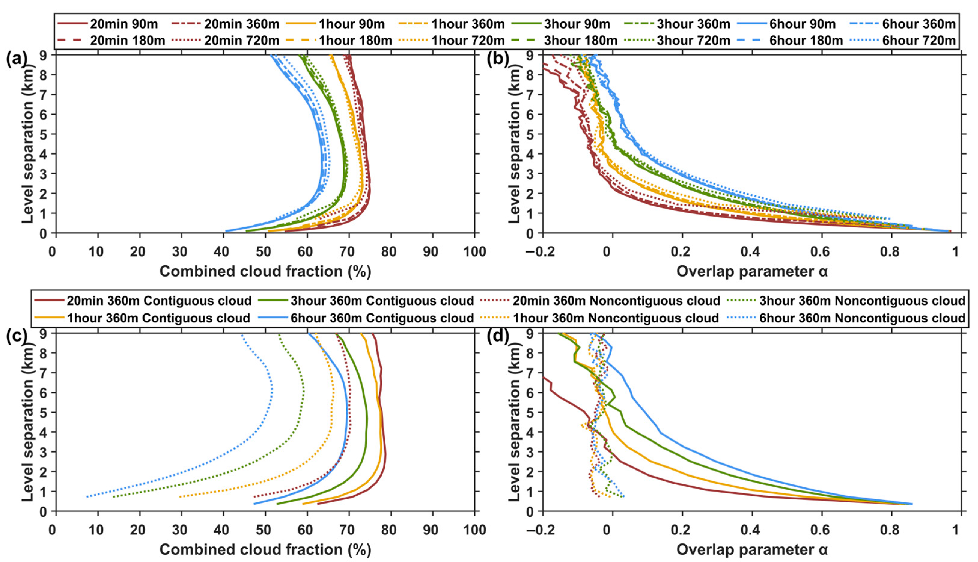
3.1.1. Spatial and Temporal Resolution Effects on Cloud Overlap

Cloud occurrence and fraction values vary at different spatial and temporal resolutions; thus, the first step in this study is to determine the appropriate spatial and temporal resolution. Figure 2a,b shows the difference between cloud occurrence and fraction vertical distribution under various temporal resolutions (20 min, 1 h, 3 h, and 6 h) and vertical spatial resolutions (90 m, 180 m, 360 m, and 720 m). Both cloud occurrence and fraction have their maximum at high altitudes around 9 km above sea level. The influence of temporal resolution on the vertical distribution of cloud occurrence and fraction is more significant compared to that of vertical spatial resolution. Enhancing the vertical spatial resolution (from 720 m to 90 m) results in a slight reduction in cloud occurrence and fraction. With an increase in temporal resolution ranging from 6 h to 20 min, cloud occurrence shows a decrease trend in the overall, while simultaneously CF increases. Figure 2c shows that in the all-cloud scenario, 95% of the cloud layer pairs have Δz of less than 8 km, while in the contiguous cloud scenario, the threshold of height is 7 km, as shown in Figure 2d.
In order to quantitatively characterize cloud overlap properties, we can describe them by three characteristic factors: Lcf, Ctrue, and α. In addition, we discuss different cloud scenarios, i.e., all cloud layers, contiguous cloud layers, and six cloud types. The six cloud types are classified by the altitude of the cloud top and base, including low clouds (L), middle clouds (M), high clouds (H), low-middle clouds (LM), middle-high clouds (MH), and low-middle-high clouds (LMH). Specifically, the Lcf for different cloud categories with different spatial and temporal resolutions is listed in Table 1. It is obvious that Lcf increases with decreasing spatial and temporal resolution, and the changes caused by different temporal resolutions are more significant than those of spatial resolutions. Ctrue mainly increases uniformly from 40% to 75% with Δz increasing in Figure 3a, while α decreases from 1 to −0.2 in Figure 3b. Similarly, the effect of vertical spatial resolution is relatively minor compared to the effect of temporal resolution for Ctrue and α.
The optimal vertical spatial resolution for cloud overlap studies is determined to be 360 m based on a comprehensive analysis of theoretical and empirical factors. Firstly, cloud modeling in ERA5 and CMIP6 typically involves a minimum pressure level range of 25 hPa, equivalent to approximately 500 m at elevated elevations [37,38]. Secondly, the multi-layer cloud algorithm of KAZR has the precondition that the distance between adjacent cloud layers must be greater than 300 m. Thirdly, the CloudSat satellite utilized in this study offers a vertical resolution of 240 m. Considering these factors, a vertical resolution of 360 m is deemed appropriate as it aligns with the numerical parameters outlined above.
Under this vertical resolution condition, we analyze the overlapping clouds for contiguous and noncontiguous cloud layers at different temporal resolutions (Figure 3c,d). Enhancing the temporal resolution amplifies the variability of Ctrue, especially for noncontiguous cloud layers. The distribution of α is found to be uniformly dispersed around 0, indicating a typical representation of random overlap. For contiguous cloud layers, the distributions of Ctrue and α in Figure 3c,d are consistent with those in Figure 3a,b, particularly under the temporal resolution of 20 min and 1 h. When Δz increases, Ctrue gradually increases and then remains stable, suggesting a shift from maximum to random overlap in the actual overlap approach. As the time resolution decreases (from 20 min to 6 h), simulating overlapping cloud fractions becomes more difficult. In addition, there is a lower possibility of data truncation and a higher percentage of valid samples for 1 h resolution compared to 20 min resolution (revealed in Figure 2). Therefore, 1 h is the appropriate time resolution. In summary, the following analysis will be performed at a resolution of 1 h and 360 m.

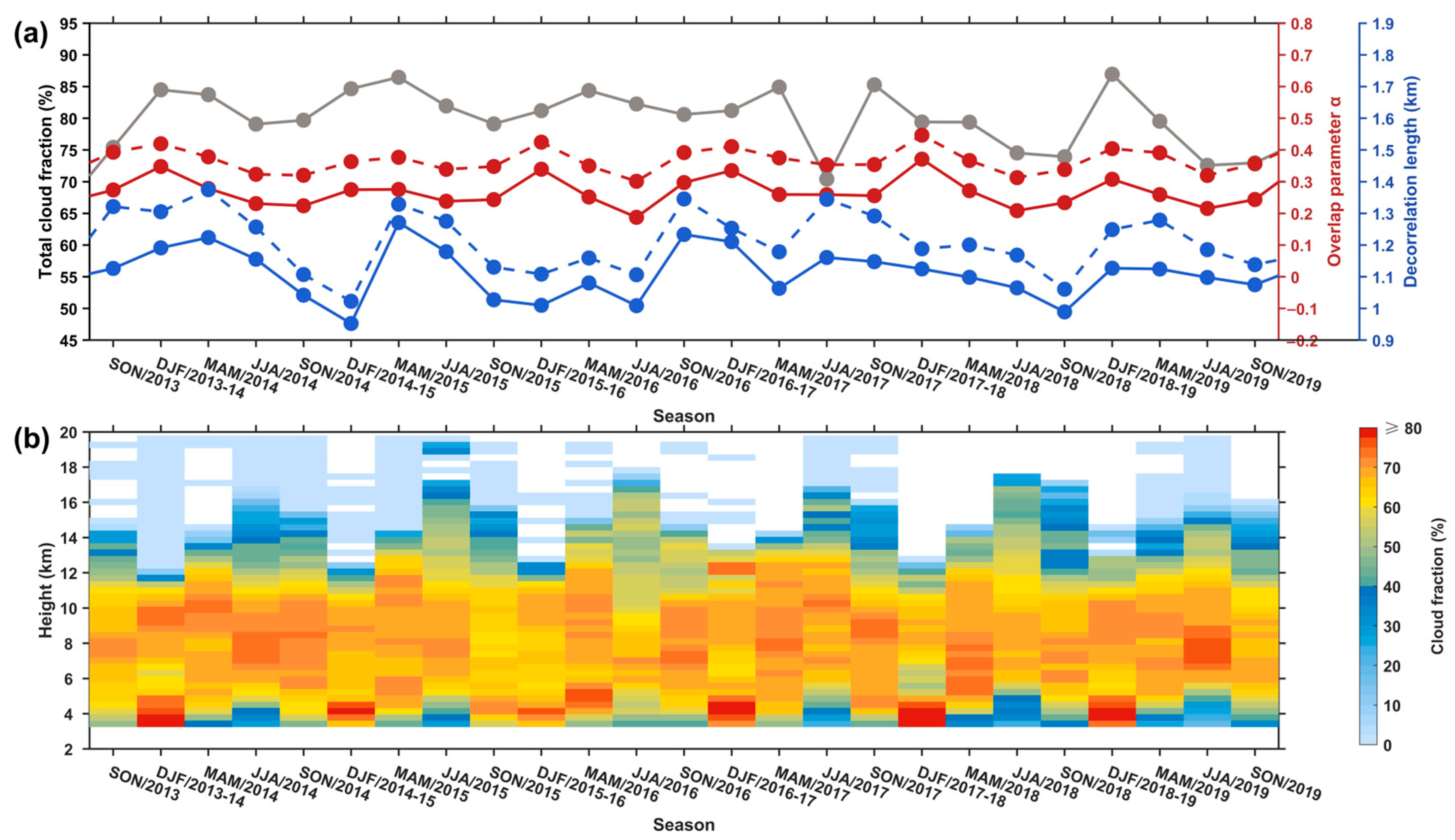
3.1.2. Seasonal Variations of Cloud Overlap

The seasonal variations of cloud parameters (i.e., TCF, α, and Lcf) and the vertical distribution of CF from 2013 to 2019 with resolutions of 1 h and 360 m are shown in Figure 4a,b, respectively. In Figure 4a, it can be seen that the cloud parameter of all cloud layers (solid lines) is always smaller than that of the continuous cloud layers (dotted lines) in any season, indicating that the cloud layer tends to random overlap in the vertical direction. The increasing (decreasing) TCF corresponds to the clouds random overlap weakening (strengthening), which is consistent with the sensitivity of TCF to the cloud overlap categories as proposed by Li et al. [5]. α and TCF exhibit seasonal periodicity, with their values reaching high levels during winter (December-January-February, DJF) and spring (March-April-May, MAM) and dropping to low levels during summer (June-July-August, JJA) and autumn (September-October-November, SON). When TCF reaches its extremes, Lcf usually lags one or two seasons before reaching its maximum or minimum, and there is a negative correlation between them (correlation coefficient: −0.54~−0.66). Furthermore, the trend of TCF seasonal variation exhibits synchronicity with α and inconsistency with Lcf, which may be attributed to the negative correlation between TCF and Lcf. We also analyze the CF at different altitudes with seasonal variation, as shown in Figure 4b. It is evident that the altitude at which the maximum CF occurs varies significantly from season to season. The maximum CF (>80%) in winter is mainly concentrated below 5 km, while in other seasons, it is concentrated in the range of 5–10 km. Especially in Figure 4b summer (June-July-August, JJA), less CF is observed at both lower altitudes (near the ground) and higher altitudes (more than 15 km) than in other seasons, which may be related to the strong convective cloud system with abundant water vapor and unstable thermal structure in summer.

3.1.3. Comparison of Cloud Overlaps for Different Cloud Types

Cloud overlap characteristics vary with cloud types, and it is of great significance to develop various cloud overlap schemes for different cloud types to improve the cloud parameterization in models. Therefore, we classify the cloud layer into six types according to the average of cloud base height (CBH) and cloud top height (CTH), as proposed by Xi et al. [39] and Dong et al. [40]. The six cloud types (Figure 5a) include low clouds (CTH ≤ 5 km, L), middle clouds (CTH ≤ 8 km and CBH > 5 km, M), high clouds (CBH > 8 km, H), low-middle clouds (5 km < CTH ≤ 8 km and CBH ≤ 5 km, LM), middle-high clouds (CTH > 8 km and 5 km < CBH ≤ 8 km, MH), and low-middle-high clouds (CTH > 8 km and CBH ≤ 5 km, LMH). In addition, the frequency of different cloud types does not show significant variations with distinct temporal resolution (Figure 5b), which further confirms that it is feasible to analyze cloud parameters for different cloud types with 1 h resolution.
For six different cloud types, we statistically analyze the seasonal variation of total cloud occurrence (TCO) (Figure 5c) and TCF (Figure 5d). The TCO of LMH clouds is mainly concentrated at 63~86%, with the maximum occurring in September and the minimum in December. The TCO of M clouds is the lowest, less than 10%, while the TCO of MH clouds is the highest, greater than 20%. This suggests that MH clouds are the dominant cloud type in the arid and semi-arid regions represented by the SACOL station. On the other hand, the TCF of L clouds shows a trend of gradually decreasing and then rising with the monthly variations. Notably, a valley value of TCF for different cloud types is observed around July. This can be attributed to the presence of abundant water vapor and the formation of multiple cumulus clouds due to convection in the summer, while the dominance of stratus clouds is influenced by frontal systems in the winter.
When the cloud layers are vertically contiguous, we conduct calculations on α and the combined cloud fraction (Ctrue, Cmin, Crand, Cmax) for different cloud types. Figure 6 reveals the cloud overlap characteristics of these six cloud types. Firstly, α decreases as Δz increases for all types of clouds, and the rate of reduction in this parameter slows down when Δz exceeds 2 km. The decreasing α indicates a reduction in the degree of overlap for contiguous cloud layers. Meanwhile, the combined cloud fraction of L and H clouds monotonically increases as Δz expands, while that of other cloud types exhibits a trend of initially increasing and then decreasing, with extreme values occurring at 1.5 km (H), 3 km (LM, MH), and 3–5 km (LMH), respectively. However, the Ctrue for all cloud types shows a shift from Cmax to Crand, similar to previous studies [10,23]. In addition, the calculation of α is related to the combined cloud fraction. When α < 0, the Ctrue lies between the Cmin and the Crand (Crand < Ctrue < Cmin); conversely, when α > 0, it is distributed between the Cmax and the Crand (Cmax < Ctrue < Crand). Relative to the actual combined cloud fraction of different cloud types, the cloud fraction bias of the minimum and random overlap assumptions is positive, and that of the maximum overlap assumption is negative. In detail, the minimum bias of the cloud fraction for L, M, and H clouds is from maximum overlap, and that of LM, MH, and LMH is from random overlap.

3.2. Comparison of KAZR and Satellite Observed Cloud Overlaps

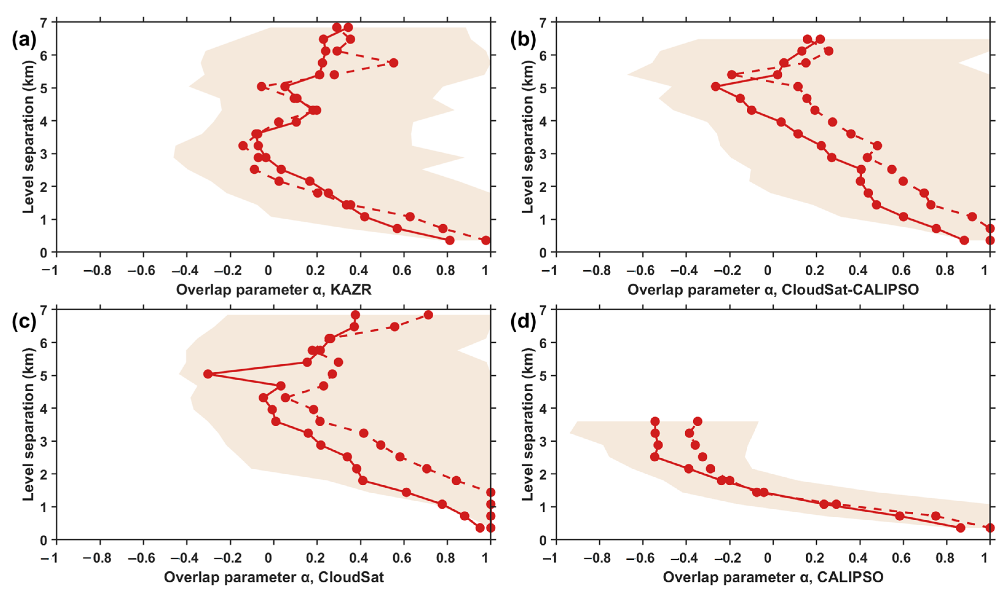
3.2.1. Analysis of Evaluation Area and Cloud Overlap Parameters from Various Products

Different probing techniques of multiple instruments have different spatial coverage, and it is possible that some clouds can only be seen by one instrument but are invisible to others. In addition to the different observation areas of similar instruments, the greater differences come from the variety of observation platforms. Ground-based and space-borne instruments provide continuous observations of single points and instantaneous observations of a space region, respectively. Before the formal comparison, this section needs to discuss cloud homogeneity within different instrument observational fields, and it is necessary to determine the appropriate time-space field, containing the time window and this study area. We chose 1 h as the temporal resolution and selected 0.2° × 0.2° − 1.0° × 1.0° around SACOL as this research area to constrain that only one satellite orbit passes within this region, as shown in Figure 7a. Then, the most suitable region are selected by comparing the TCF and its correlation with different observation data in each region. Figure 7b shows that the TCF of all observed data at 0.7° × 0.7° exhibits a decreasing inflection point. In the meantime, the correlation coefficient of CF between MODIS and active observation displays two peaks at 0.5° × 0.5° and 0.7° × 0.7° (Figure 7c). Similarly, the association of CF between KAZR and satellite observation is stronger in this range (Figure 7d). Consequently, based on the time resolution of 1 h, we designate the optimal area as 0.7° × 0.7°. The analysis of the evaluation area facilitates screening these samples with effective cloud observations and prevents scenarios where some clouds are visible only to one instrument. We then statistically analyze 42 effective cloud observation cases within this spatiotemporal field, as detailed in Table 2.
These cases prevent scenarios where some clouds are visible only to one instrument.
Based on the above cases, we carried out a cloud overlap comparison of active observations from the CloudSat-CALIPSO, CloudSat, CALIPSO, and KAZR datasets. Two points require attention: (1) For all cloud layer pairs from different datasets, the proportion of noncontiguous clouds are significantly less than that of contiguous clouds. Therefore, we will focus on investigating the characteristics of contiguous clouds as representative examples. (2) Considering the data dispersion caused by the sample reduction, both the average and median of the cloud overlap parameter corresponding to different Δz are retained.
Figure 8 shows the α and Δz distributions of contiguous cloud pairs from different products. The average and median of α changes from different products show a consistent trend. Specifically, the α shows a decreasing and then increasing trend as the Δz increases, indicating the initial strengthening and subsequent weakening of random overlap. The smaller cloud overlap parameter means that the real overlapping cloud amount is larger than the random overlapping cloud amount, or the maximum overlapping cloud amount is less different from the random overlapping cloud amount, which reflects the low degree of cloud overlap and the large difference in cloud amount. For different Δz, the relative differences between the average and median cloud overlap parameters of KAZR are relatively small, whereas those of the satellite products are slightly larger. This suggests that satellite observations depict a cloud distribution that is more non-uniform, capturing additional minimal values of the cloud overlap parameter. In detail, for KAZR, the α decreases from 1 to 0 when Δz increases to 4 km and then increases to 0.3 as Δz continues to increase, which is consistent with Figure 3d. For CloudSat-CALIPSO, the cloud overlap parameter also decreases and then increases as increasing Δz, where the decreasing and increasing intervals of the average (median) cloud overlap parameter are located at 0.9~−0.3 (1.0~−0.2) and −0.3~0.2 (−0.2~0.2), respectively. For CloudSat, the average (median) cloud overlap parameter ranges from 1 to −0.4 (from 1.0 to 0) when Δz increases to 5 km (4 km) and from −0.4 to 0.4 (from 0 to 0.7) when Δz keeps increasing, respectively. Comparatively, for CALIPSO, the Δz lies within 4 km, and the average (median) cloud overlap parameter varies from 0.9 to −0.5 (from 1.0 to −0.4) with increasing Δz. The reasons contributing to the large departure of CALIPSO results from others are: (1) The lidar signal is easier to attenuate and harder to penetrate clouds with thicker optical thickness, resulting in a narrower Δz; (2) The lidar signal is sensitive to smaller cloud particles and easier to retrieve thinner clouds, resulting in a smaller negative α.

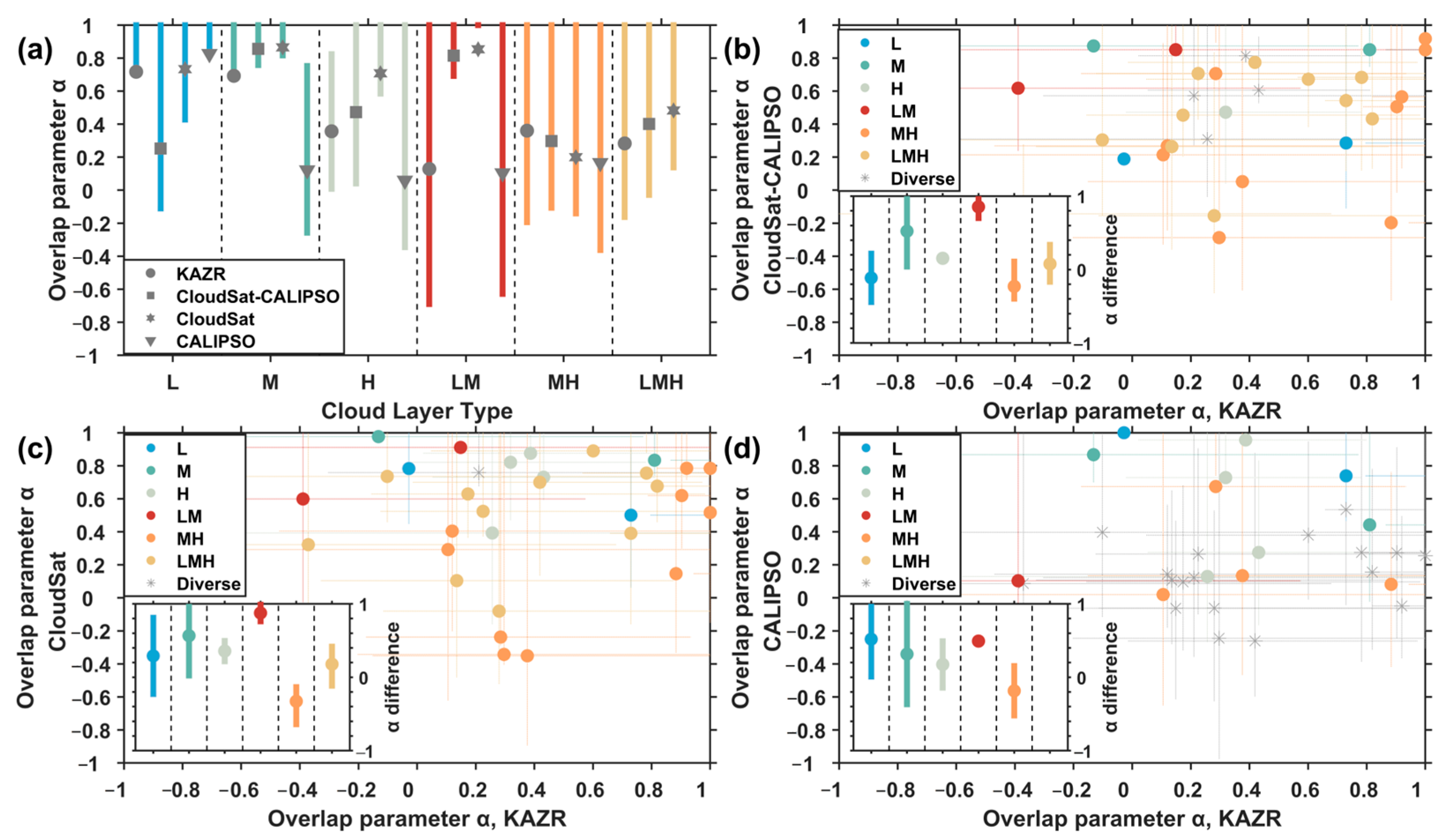
3.2.2. Evaluation of the Cloud Overlap Parameter for Different Cloud Types

Based on the above conditions, we perform the statistical analysis of different cloud types based on overlap characteristics to evaluate quantitative differences among multiple datasets. Multiple instrumental observations may differ when inhomogeneous clouds exist, and to minimize discrepancy, the cases covered in this subsection need to satisfy the condition that the same cloud classification are judged by more than three datasets simultaneously (e.g., cases except code 5, 9, 10, 18, 21, 30, 31, 32, and 38 listed in Table 2). Table 2 presents the cloud types for different datasets, where the proportion of H and LMH clouds are greater for KAZR (67%), CloudSat-CALIPSO (76%), and CloudSat (67%), while CALIPSO, which cannot determine LMH clouds due to lidar signal attenuation, retrieves up to 73% of MH and H clouds. In addition, noting the limited sample of cloud types identified by multiple instruments, the variation description of the cloud overlap parameter will be more intuitive than the computational characterization of decorrelation length when comparatively analyzing cloud overlap characteristics.
Figure 9 illustrates the variation of the cloud overlap parameter for different cloud types with increasing Δz in various datasets. For the CALIPSO dataset, the cloud overlap parameter decreases gradually with larger Δz for all cloud types (M, H, LM, and MH clouds). When Δz exceeds 1.5 km, the cloud overlap parameter is less than 0. Apart from the CALIPSO dataset, the cloud overlap parameter for LMH clouds shows different trends at Δz above and below 4–5 km. It decreases at Δz above 4–5 km and increases at Δz below 4–5 km. The cloud overlap parameter for L and M clouds is mainly concentrated around 1. For LM clouds, each dataset corresponds to the maximum overlap assumption at Δz of approximately 1 km. When the Δz exceeds 3 km, the cloud overlap parameter is negative for KAZR, while it is positive for CloudSat-CALIPSO and CloudSat retrievals. This discrepancy is due to the differences between satellite and ground-based instrument observations or the interference of near-surface clutter with low-level cloud retrieval. Furthermore, for MH clouds, the positive and negative divisions of the cloud overlap parameter correspond to Δz of around 3 km for KAZR and CloudSat-CALIPSO retrievals, while for CloudSat it is around 2.5 km.
Figure 10 reveals the quantitative differences in the cloud overlap parameter for different cloud types retrieved by multiple datasets. The average and interquartile cloud overlap parameters for different datasets are shown in Figure 10a. For MH and LMH clouds, the average cloud overlap parameter of different datasets lies at 0.17~0.36 and 0.28~0.48, respectively. The dataset that most closely resembles KAZR in terms of the cloud overlap parameter is CloudSat-CALIPSO. For LM clouds, the average cloud overlap parameter of KAZR (CALIPSO) is 0.13 (0.10) and that of CloudSat-CALIPSO (CloudSat) is 0.81 (0.85), reflecting that KAZR and CALIPSO retrieve lower clouds with less overlap degree, which also supports the speculation for LM clouds in Figure 9. Additionally, this study quantifies the differences in the cloud overlap parameter between satellites and KAZR. In Figure 10b, CloudSat-CALIPSO and KAZR exhibit 88% agreement in cloud type identification, with discrepancies primarily arising from H clouds of KAZR being judged as MH clouds of CloudSat-CALIPSO. In Figure 10c, CloudSat and KAZR have the same cloud type in the majority of cases, and only 3% of cases show a discrepancy where KAZR and CloudSat identify LMH and MH clouds. In Figure 10d, a notable disparity in cloud classification is observed between CALIPSO and KAZR. Specifically, LMH clouds (MH clouds) identified by KAZR are categorized as MH and H clouds (M and H clouds) by CALIPSO, accounting for 37% (19%) of all cases. In addition, based on cases where satellite and KAZR agree on the cloud type simultaneously, we calculate the mean differences in the cloud overlap parameter. As depicted in the nested subplots of Figure 10b–d, the mean differences in the cloud overlap parameter between satellites and KAZR are generally smaller for H, MH, and LMH clouds. Specifically, the mean differences of H clouds (MH clouds) are 0.15 (−0.23) for CloudSat-CALIPSO, 0.36 (−0.33) for CloudSat, and 0.17 (−0.18) for CALIPSO; for LMH clouds, the mean differences are 0.08 and 0.18 for CloudSat-CALIPSO and CloudSat. Consequently, compared to CloudSat and CALIPSO, the retrieved cloud overlap parameter closest to the ground-based KAZR is the joint data product of CloudSat and CALIPSO.

4. Discussion and Conclusions

This study investigates the dependence of cloud overlap properties on macroscopic conditions at the SACOL site and quantifies the difference in multiple datasets. Specifically, this study utilizes the continuous observation of cloud vertical structure from KAZR to investigate the cloud overlap characteristics represented by the SACOL site with the potential impacts including temporal-spatial scale, TCF, seasonal variations, and cloud classification. In addition to ground-based observation, this study also combines cloud profile observations from satellites’ datasets (i.e., 2B-CLDCLASS, L2-01kmClay, and 2B-CLDCLASS-LIDAR) and compares their cloud overlap characteristics quantitatively, considering the impact of the appropriate study area, involved study cases, and different cloud types. The significance of this paper lies in the fact that statistical analysis of continuous observations reflecting spatial and temporal variation characteristics is essential for the improvement of cloud parameterization schemes, and comparative analysis of multiple observations is beneficial for providing an effective datum foundation.
Using the continuous vertical cloud data from KAZR, based on the limitations of the model and observation on vertical resolution as well as the effect of temporal resolution on CF and sample size, the resolution for cloud overlap studies is determined to be 1 h and 360 m. On this basis, the combined cloud fraction bias of the random overlap assumption is the smallest for contiguous and noncontiguous clouds. Meanwhile, when the Δz is small (i.e., less than 1 km), the minimum bias for contiguous clouds stems from the maximum cloud overlap assumption, while for noncontiguous clouds, it arises from the minimum cloud overlap assumption. In addition, the TCF and cloud overlap properties show a significant trend in the seasonal variations. Specifically, the seasonal variation of the cloud overlap parameter and TCF is maximized in winter-spring and minimized in summer-autumn, and that of the decorrelation length lags behind by one or two seasons. In addition to the seasonal periodicity, the overlap properties of different cloud types also exhibit significant differences. For L and H clouds, the combined cloud fraction monotonically increases as the Δz expands, while the CFs of the four remaining cloud types exhibit a trend of initially increasing and then decreasing, with extreme values occurring at 1.5 km (H), 3 km (LM, MH), and 3–5 km (LMH).
The comparison of cloud overlap properties utilizes multiple datasets, including ground-based (KAZR) and satellite-based observations (including CloudSat, CALIPSO, and combined CloudSat-CALIPSO products). To ensure different datasets cover effective cloud observation, the correlation of TCF between ground-based and satellite-based observations (between active and passive remote observations) are discussed as a function of this study area, and the appropriate study area is determined to be 0.7° × 0.7° centered on the SACOL site. The specific cases involved in this study are also counted quantitatively. Based on the aforementioned analysis, when layer separation increases, the cloud overlap parameter of different datasets decreases initially and then increases, which corresponds to random overlap strengthening and weakening, respectively. In addition, inhomogeneous clouds exist frequently in the satellite viewing range when layer separation is unified: for ground-based observations, the difference between the average and median of the cloud overlap parameter is small; for satellite-based observations, the median is slightly greater than the average. Quantitatively, the average of the cloud overlap parameter is utilized to calculate Lcf: KAZR is 1.43 km, Cloudsat-CALIPSO is 2.18 km, Cloudsat is 2.58 km, and CALIPSO is 1.11 km. Relative to CloudSat and CALIPSO, the average cloud overlap from CloudSat-CALIPSO is closest to that from KAZR, especially for the largest proportion of H, MH, and LMH clouds. For low-level clouds (i.e., L, M, and LM) with Δz less than 1 km, the CF error is minimized in the maximum overlap assumption for all datasets in this study.

Author Contributions

Conceptualization, J.G. and X.Y.; methodology, X.Y.; software, X.Y.; validation, X.Y., Q.L., J.G., B.W., N.P. and J.S.; formal analysis, X.Y.; investigation, X.Y.; resources, X.Y.; data curation, X.Y.; writing—original draft preparation, X.Y.; writing—review and editing, X.Y., Q.L., J.G., C.Z. and J.D.; visualization, X.Y.; supervision, J.G.; project administration, J.G.; funding acquisition, J.G. All authors have read and agreed to the published version of the manuscript.

Funding

This research was funded by the National Science Foundation of China (grants 42275076 and 41922032), the Science and Technology Project of Gansu Province (grant 22JR5RA446), and the Fundamental Research Funds for the Central Universities (grant lzujbky-2022-ct06).

Data Availability Statement

The data were obtained from NASA Level-1 and the Atmosphere Archive and Distribution System Distributed Active Archive Center (MODIS Aqua, https://ladsweb.modaps.eosdis.nasa.gov/, accessed on 20 July 2022), the NASA Langley Research Center Atmospheric Science Data Center (CALIPSO, https://eosweb.larc.nasa.gov/project/calipso/calipso_table, accessed on 20 July 2022), the NASA CloudSat data processing center (CloudSat, http://www.cloudsat.cira.colostate.edu/direct-ftp-access, accessed on 20 July 2022), and the SACOL data archive (KAZR, http://climate.lzu.edu.cn, accessed on 20 July 2022).

Acknowledgments

We thank the science teams of MODIS Aqua, CloudSat, CALIPSO, and KAZR for providing excellent and accessible data that made this study possible.

Conflicts of Interest

The authors declare no conflicts of interest.

References

  1. Garay, M.J.; de Szoeke, S.P.; Moroney, C.M. Comparison of marine stratocumulus cloud top heights in the southeastern Pacific retrieved from satellites with coincident ship-based observations. J. Geophys. Res. Atmos. 2008, 113, D18204. [Google Scholar] [CrossRef]
  2. Ge, J.; Wang, Z.; Wang, C.; Yang, X.; Dong, Z.; Wang, M. Diurnal variations of global clouds observed from the CATS spaceborne lidar and their links to large-scale meteorological factors. Clim. Dyn. 2021, 57, 2637–2651. [Google Scholar] [CrossRef]
  3. Yang, X.; Ge, J.; Hu, X.; Wang, M.; Han, Z. Cloud-Top Height Comparison from Multi-Satellite Sensors and Ground-Based Cloud Radar over SACOL Site. Remote Sens. 2021, 13, 2715. [Google Scholar] [CrossRef]
  4. Forster, P.; Storelvmo, T.; Armour, K.; Collins, W.; Dufresne, J.L.; Frame, D.; Lunt, D.J.; Mauritsen, T.; Palmer, M.D.; Watanabe, M.; et al. The Earth’s Energy Budget, Climate Feedbacks, and Climate Sensitivity. In Climate Change 2021: The Physical Science Basis. Contribution of Working Group I to the Sixth Assessment Report of the Intergovernmental Panel on Climate Change; Masson-Delmotte, V., Zhai, P., Pirani, A., Connors, S.L., Péan, C., Berger, S., Caud, N., Chen, Y., Goldfarb, L., Gomis, M.I., et al., Eds.; Cambridge University Press: Cambridge, UK; New York, NY, USA, 2021; pp. 923–1054. [Google Scholar]
  5. Li, J.; Jian, B.; Zhao, C.; Zhao, Y.; Wang, J.; Huang, J. Atmospheric Instability Dominates the Long-Term Variation of Cloud Vertical Overlap Over the Southern Great Plains Site. J. Geophys. Res. Atmos. 2019, 124, 9691–9701. [Google Scholar] [CrossRef]
  6. Wang, H.B.; Zhang, H.; Xie, B.; Jing, X.W.; He, J.Y.; Liu, Y. Evaluating the Impacts of Cloud Microphysical and Overlap Parameters on Simulated Clouds in Global Climate Models. Adv. Atmos. Sci. 2022, 39, 2172–2187. [Google Scholar] [CrossRef]
  7. Naud, C.M.; Del Genio, A.; Mace, G.G.; Benson, S.; Clothiaux, E.E.; Kollias, P. Impact of dynamics and atmospheric state on cloud vertical overlap. J. Clim. 2008, 21, 1758–1770. [Google Scholar] [CrossRef]
  8. Lipat, B.R.; Voigt, A.; Tselioudis, G.; Polvani, L.M. Model Uncertainty in Cloud–Circulation Coupling, and Cloud-Radiative Response to Increasing CO2, Linked to Biases in Climatological Circulation. J. Clim. 2018, 31, 10013–10020. [Google Scholar] [CrossRef]
  9. Sulak, A.M.; Calabrase, W.J.; Ryan, S.D.; Heus, T. The Contributions of Shear and Turbulence to Cloud Overlap for Cumulus Clouds. J. Geophys. Res. Atmos. 2020, 125, e2019JD032017. [Google Scholar] [CrossRef]
  10. Li, J.; Lv, Q.; Jian, B.; Zhang, M.; Zhao, C.; Fu, Q.; Kawamoto, K.; Zhang, H. The impact of atmospheric stability and wind shear on vertical cloud overlap over the Tibetan Plateau. Atmos. Chem. Phys. 2018, 18, 7329–7343. [Google Scholar] [CrossRef]
  11. Di Giuseppe, F.; Tompkins, A.M. Generalizing Cloud Overlap Treatment to Include the Effect of Wind Shear. J. Atmos. Sci. 2015, 72, 2865–2876. [Google Scholar] [CrossRef]
  12. Jing, X.W.; Zhang, H.; Peng, J.; Li, J.N.; Barker, H.W. Cloud overlapping parameter obtained from CloudSat/CALIPSO dataset and its application in AGCM with McICA scheme. Atmos. Res. 2016, 170, 52–65. [Google Scholar] [CrossRef]
  13. Tompkins, A.M.; Di Giuseppe, F. An Interpretation of Cloud Overlap Statistics. J. Atmos. Sci. 2015, 72, 2877–2889. [Google Scholar] [CrossRef]
  14. Zhang, H.; Jing, X.; Li, J. Application and evaluation of a new radiation code under McICA scheme in BCC_AGCM2.0.1. Geosci. Model Dev. 2014, 7, 737–754. [Google Scholar] [CrossRef]
  15. Jing, X.; Zhang, H.; Satoh, M.; Zhao, S. Improving Representation of Tropical Cloud Overlap in GCMs Based on Cloud-Resolving Model Data. J. Meteorol. Res. 2018, 32, 233–245. [Google Scholar] [CrossRef]
  16. Zhang, H.; Jing, X. Advances in studies of cloud overlap and its radiative transfer in climate models. J. Meteorol. Res. 2016, 30, 156–168. [Google Scholar] [CrossRef]
  17. Hill, P.G.; Morcrette, C.J.; Boutle, I.A. A regime-dependent parametrization of subgrid-scale cloud water content variability. Q. J. R. Meteorol. Soc. 2015, 141, 1975–1986. [Google Scholar] [CrossRef]
  18. Barker, H.W. Overlap of fractional cloud for radiation calculations in GCMs: A global analysis using CloudSat and CALIPSO data. J. Geophys. Res. Atmos. 2008, 113, D00A01. [Google Scholar] [CrossRef]
  19. Barker, H.W. Representing cloud overlap with an effective decorrelation length: An assessment using CloudSat and CALIPSO data. J. Geophys. Res. Atmos. 2008, 113, D24205. [Google Scholar] [CrossRef]
  20. Wu, X.Q.; Liang, X.Z. Radiative effects of cloud horizontal inhomogeneity and vertical overlap identified from a monthlong cloud-resolving model simulation. J. Atmos. Sci. 2005, 62, 4105–4112. [Google Scholar] [CrossRef]
  21. Chen, T.; Zhang, Y.C.; Rossow, W.B. Sensitivity of atmospheric radiative heating rate profiles to variations of cloud layer overlap. J. Clim. 2000, 13, 2941–2959. [Google Scholar] [CrossRef]
  22. Hogan, R.J.; Illingworth, A.J. Deriving cloud overlap statistics from radar. Q. J. R. Meteorol. Soc. 2000, 126, 2903–2909. [Google Scholar] [CrossRef]
  23. Mace, G.G.; Benson-Troth, S. Cloud-layer overlap characteristics derived from long-term cloud radar data. J. Clim. 2002, 15, 2505–2515. [Google Scholar] [CrossRef]
  24. Wang, L.K.; Dessler, A.E. Instantaneous cloud overlap statistics in the tropical area revealed by ICESat/GLAS data. Geophys. Res. Lett. 2006, 33, L15804. [Google Scholar] [CrossRef]
  25. Kato, S.; Sun-Mack, S.; Miller, W.F.; Rose, F.G.; Chen, Y.; Minnis, P.; Wielicki, B.A. Relationships among cloud occurrence frequency, overlap, and effective thickness derived from CALIPSO and CloudSat merged cloud vertical profiles. J. Geophys. Res. Atmos. 2010, 115, D00H28. [Google Scholar] [CrossRef]
  26. Ge, J.; Zhu, Z.; Zheng, C.; Xie, H.; Zhou, T.; Huang, J.; Fu, Q. An improved hydrometeor detection method for millimeter-wavelength cloud radar. Atmos. Chem. Phys. 2017, 17, 9035–9047. [Google Scholar] [CrossRef]
  27. Hu, X.; Ge, J.; Du, J.; Li, Q.; Huang, J.; Fu, Q. A robust low-level cloud and clutter discrimination method for ground-based millimeter-wavelength cloud radar. Atmos. Meas. Tech. 2021, 14, 1743–1759. [Google Scholar] [CrossRef]
  28. Xin, Y.S.J.; Li, X.G. Retrieval of ice cloud microphysical properties at the SACOL. Chin. Sci. Bull. 2019, 64, 2728–2740. (In Chinese) [Google Scholar] [CrossRef]
  29. Winker, D.M.; Pelon, J.; Coakley, J.A.; Ackerman, S.A.; Charlson, R.J.; Colarco, P.R.; Flamant, P.; Fu, Q.; Hoff, R.M.; Kittaka, C.; et al. THE CALIPSO MISSION A Global 3D View of Aerosols and Clouds. Bull. Am. Meteorol. Soc. 2010, 91, 1211–1229. [Google Scholar] [CrossRef]
  30. Stephens, G.L.; Vane, D.G.; Tanelli, S.; Im, E.; Durden, S.; Rokey, M.; Reinke, D.; Partain, P.; Mace, G.G.; Austin, R.; et al. CloudSat mission: Performance and early science after the first year of operation. J. Geophys. Res. Atmos. 2008, 113, D00A18. [Google Scholar] [CrossRef]
  31. Sassen, K.; Wang, Z. Classifying clouds around the globe with the CloudSat radar: 1-year of results. Geophys. Res. Lett. 2008, 35, L04805. [Google Scholar] [CrossRef]
  32. Ackerman, S.A.; Holz, R.E.; Frey, R.; Eloranta, E.W.; Maddux, B.C.; McGill, M. Cloud detection with MODIS. Part II: Validation. J. Atmos. Ocean. Technol. 2008, 25, 1073–1086. [Google Scholar] [CrossRef]
  33. Platnick, S.; King, M.D.; Ackerman, S.A.; Menzel, W.P.; Baum, B.A.; Riédi, J.C.; Frey, R.A. The MODIS cloud products: Algorithms and examples from Terra. IEEE Trans. Geosci. Remote Sens. 2003, 41, 459–473. [Google Scholar] [CrossRef]
  34. Guenther, B.; Xiong, X.; Salomonson, V.V.; Barnes, W.L.; Young, J. On-orbit performance of the Earth Observing System Moderate Resolution Imaging Spectroradiometer; first year of data. Remote Sens. Environ. 2002, 83, 16–30. [Google Scholar] [CrossRef]
  35. Bergman, J.W.; Rasch, P.J. Parameterizing vertically coherent cloud distributions. J. Atmos. Sci. 2002, 59, 2165–2182. [Google Scholar] [CrossRef]
  36. Zhang, H.; Peng, J.; Jing, X.; Li, J. The features of cloud overlapping in Eastern Asia and their effect on cloud radiative forcing. Sci. China Earth Sci. 2013, 56, 737–747. [Google Scholar] [CrossRef]
  37. Hersbach, H.; Bell, B.; Berrisford, P.; Hirahara, S.; Horányi, A.; Muñoz-Sabater, J.; Nicolas, J.; Peubey, C.; Radu, R.; Schepers, D.; et al. The ERA5 global reanalysis. Q. J. R. Meteorol. Soc. 2020, 146, 1999–2049. [Google Scholar] [CrossRef]
  38. Eyring, V.; Bony, S.; Meehl, G.A.; Senior, C.A.; Stevens, B.; Stouffer, R.J.; Taylor, K.E. Overview of the Coupled Model Intercomparison Project Phase 6 (CMIP6) experimental design and organization. Geosci. Model Dev. 2016, 9, 1937–1958. [Google Scholar] [CrossRef]
  39. Xi, B.; Dong, X.; Minnis, P.; Khaiyer, M.M. A 10 year climatology of cloud fraction and vertical distribution derived from both surface and GOES observations over the DOE ARM SPG site. J. Geophys. Res. Atmos. 2010, 115, D12124. [Google Scholar] [CrossRef]
  40. Dong, X.; Xi, B.; Minnis, P. A climatology of midlatitude continental clouds from the ARM SGP central facility. Part II: Cloud fraction and surface radiative forcing. J. Clim. 2006, 19, 1765–1783. [Google Scholar] [CrossRef]
Figure 1. (a) A schematic of cloud layer modularization. The blue lines represent the observing profiles of radar or lidar, and the red markers indicate these profiles with or without clouds. (b) A schematic of cloud fraction calculation for different cloud layers, including single-cloud layer (Layer 1), two-cloud layer (Layer 1 and 2), and all-cloud layer (Layer 1, 2, and 3).
Remotesensing 16 00218 g001
Figure 2. (a) The available cloud occurrence and (b) the mean cloud fraction within the difference height range (above sea level, a.s.l.) vary with temporal and spatial resolution. The cumulative distribution function (CDF) and probability density function (PDF) of the level separation (Δz) for (c) all cloud layer pairs and (d) contiguous cloud layer pairs. The dotted lines are added to emphasize the PDF thresholds of 90% and 95% in the level separation Δz of cloud layer pairs.
Remotesensing 16 00218 g002
Figure 3. The variations with temporal and spatial resolution about the average (a) actual combined cloud fraction (Ctrue) and (b) cloud overlap parameter (α) for all cloud layer pairs. Based on a vertical resolution of 360 m, the variations with time resolution are about average (c) Ctrue and (d) α for contiguous and noncontiguous cloud pairs.
Remotesensing 16 00218 g003
Figure 4. Time series of seasonal averages about (a) total cloud fraction (TCF, gray line), cloud overlap parameter (α, red line), decorrelation length (Lcf, blue line), and (b) cloud fraction vertical profiles (above sea level, a.s.l.). The solid line represents all cloud layers, and the dotted line represents contiguous cloud layers. Different seasons cover March-April-May of spring (MAM), June-July-August of summer (JJA), September-October-November of autumn (SON), and December-January-February of winter (DJF).
Remotesensing 16 00218 g004
Figure 5. (a) Cloud classification schematic according to cloud top height (CTH) and cloud base height (CBH), including low clouds (CTH ≤ 5 km, L), middle clouds (CTH ≤ 8 km and CBH > 5 km, M), high clouds (CBH > 8 km, H), low-middle clouds (5 km < CTH ≤ 8 km and CBH ≤ 5 km, LM), middle-high clouds (CTH > 8 km and 5 km < CBH ≤ 8 km, MH), and low-middle-high clouds (CTH > 8 km and CBH ≤ 5 km, LMH). (b) Variation of different cloud-type frequencies with time resolution. Monthly variation of (c) total cloud occurrence and (d) mean total cloud fraction for different cloud types.
Remotesensing 16 00218 g005
Figure 6. The average actual and predicted combined cloud fraction (black line) of contiguous cloud layer pairs and their overlap parameter (α, red line) are performed under the premise of level separation (Δz) PDF not exceeding 95%. First column: (a) low clouds, L; (c) middle clouds, M; (e) high clouds, H. Second column: (b) low-middle clouds, LM; (d) middle-high clouds, MH; (f) low-middle-high clouds, LMH.
Remotesensing 16 00218 g006
Figure 7. (a) The map projection of the A-train constellation trajectory (blue line), the ground position of the SACOL site (red point), and its surrounding study area (red square, i.e., 0.2° × 0.2°\0.4° × 0.4°\0.6° × 0.6°\0.8° × 0.8°\1.0° × 1.0°). In different study areas, (b) the total cloud fraction and case occurrence number of each data product; (c) the correlation coefficients of total cloud fraction between passive and active observation; and (d) the correlation coefficients of total cloud fraction between ground and satellite observation. The yellow background of (b) denotes the top 80% of MODIS total cloud fraction.
Remotesensing 16 00218 g007
Figure 8. The average (solid line) and median (dotted line) cloud overlap parameter (α) for contiguous cloud layer pairs. (a) KAZR, (b) CloudSat-CALIPSO, (c) CloudSat, and (d) CALIPSO. The vertical coordinate range indicates the level separation (Δz) PDF not exceeding 95%, and the light shading represents the interquartile range (IQR) of the cloud overlap parameter.
Remotesensing 16 00218 g008
Figure 9. The average cloud overlap parameter (α) for contiguous cloud layer pairs, including different cloud types (i.e., L, M, H, LM, MH, and LMH), under the premise of level separation (Δz) PDF not exceeding 95%. (a) KAZR, (b) CloudSat-CALIPSO, (c) CloudSat, and (d) CALIPSO. Both dotted and solid lines are the fits of the inverse exponential equation (i.e., α = exp (Δz/Lcf)).
Remotesensing 16 00218 g009
Figure 10. (a) The cloud overlap parameter (α) of different products for continuous cloud layers, with dots and lines representing the mean and the interquartile range (IQR) of α, respectively. The average cloud overlapping parameter derived from KAZR and satellite observations and the difference between them (satellite minus KAZR), where lines indicate IQR, including (b) CloudSat-CALIPSO, (c) CloudSat, and (d) CALIPSO.
Remotesensing 16 00218 g010
Table 1. The decorrelation length (Lcf) of multiple cloud types under different temporal and spatial resolutions. All-cloud layer (A) and Contiguous-cloud layer (C) include multiple cloud types (i.e., L, M, H, LM, MH, and LMH). All Lcf values are performed at a level separation (Δz) PDF not exceeding 95%.
Cloud Layer TypeVertical Resolution
(m)
Temporal ResolutionCloud Layer TypeVertical Resolution
(m)
Temporal Resolution
20 min1 h3 h6 h20 min1 h3 h6 h
All-
cloud layer
900.731.011.421.75Contiguous-
cloud layer
900.811.141.611.99
1800.741.021.441.761800.821.141.602.00
3600.831.101.501.813600.891.201.642.03
7201.161.371.711.987201.171.421.802.13
(A)
L
900.420.570.851.06(C)
L
900.460.671.031.40
1800.450.590.831.011800.470.661.001.26
3600.620.750.931.023600.630.780.991.19
7201.051.171.211.297201.151.291.251.42
(A)
M
900.761.021.301.40(C)
M
900.901.221.761.82
1800.771.041.301.401800.891.221.701.79
3600.861.101.381.453600.921.241.671.71
7201.191.341.541.617201.261.441.771.80
(A)
H
900.690.891.171.47(C)
H
900.730.941.231.59
1800.720.941.201.481800.750.981.271.60
3600.871.031.311.553600.881.071.361.65
7201.191.451.571.777201.221.411.601.87
(A)
LM
900.711.021.431.80(C)
LM
900.791.161.682.19
1800.721.031.441.811800.801.161.662.18
3600.821.101.521.853600.891.231.632.13
7201.151.311.782.027201.191.411.862.23
(A)
MH
900.771.111.611.97(C)
MH
900.861.271.912.37
1800.781.121.621.981800.871.261.892.35
3600.861.201.682.033600.951.311.902.35
7201.151.431.882.157201.211.492.072.32
(A)
LMH
900.731.011.391.70(C)
LMH
900.831.141.521.81
1800.741.011.411.721800.831.141.521.83
3600.831.091.491.793600.901.191.591.89
7201.091.321.652.017201.151.411.742.07
Table 2. Cloud layer classification of 42 specific cases involved in cloud overlap comparison between KAZR and satellite observation.
CodeDateCloud Layer ClassificationCodeDateCloud Layer Classification
KAZRCloudSat CALIPSOCloudSatCALIPSOKAZRCloudSat CALIPSOCloudSatCALIPSO
102 Sep 2013HMHHH2208 Aug 2015MHMHMHM
218 Sep 2013LMLMLMM2324 Sep 2015MHMHMHH
320 Oct 2013HMHHH2410 Oct 2015MMMM
428 Mar 2014MHMHMHMH2512 Nov 2015LMHLMHLMHMH
514 Apr 2014HMHMHH2604 Apr 2016HHHH
616 May 2014LMHLMHLMHMH2720 Apr 2016MHMHMHH
704 Aug 2014LMHMHMHMH2806 Jun 2016MHMHMHH
820 Aug 2014LMHLMHLMHH2922 Jun 2016LMHLMHLMHH
904 Sep 2014LMMLM3024 Aug 2016LMHLMHLM
1020 Sep 2014LMHLMLMM3110 Sep 2016MHLMHLMHMH
1108 Nov 2014LLLL3226 Sep 2016MHMHHH
1224 Nov 2014LLLL3312 Oct 2016MHMHMHMH
1310 Dec 2014LMHLMHLMHMH3428 Oct 2016LMHLMHLMHMH
1426 Dec 2014HMHHH3512 Nov 2016MHMHMHH
1528 Jan 2015LLLL3628 Nov 2016MHMHMHM
1628 Feb 2015MHMHMHMH3704 Mar 2017LMHLMHLMHMH
1700 Apr 2015LMHLMHLMHH3820 Mar 2017MHLMHMHM
1816 Apr 2015HMHHM3924 May 2017LMHLMHLMHMH
1904 May 2015LMHLMHLMHMH4002 Dec 2017MMMM
2020 May 2015LMHLMHLMHMH4120 Dec 2018LMLMLMLM
2122 Jul 2015MHLMMM4228 Mar 2019MHMHMHMH
Disclaimer/Publisher’s Note: The statements, opinions and data contained in all publications are solely those of the individual author(s) and contributor(s) and not of MDPI and/or the editor(s). MDPI and/or the editor(s) disclaim responsibility for any injury to people or property resulting from any ideas, methods, instructions or products referred to in the content.

