Article

Stronger Impact of Extreme Heat Event on Vegetation Temperature Sensitivity under Future Scenarios with High-Emission Intensity

1
School of Ecology, Hainan University, Haikou 570000, China
2
Department of Infrastructure Engineering, The University of Melbourne, Parkville, Victoria 3010, Australia
3
Ecological Environment Monitoring Center of Hainan Province, Haikou 571126, China
4
Hainan Baoting Tropical Rainforest Ecosystem Observation and Research Station, School of Ecology, Hainan University, Haikou 570228, China
*
Author to whom correspondence should be addressed.
These authors contributed equally to this work.
Remote Sens. 2024, 16(19), 3708; https://doi.org/10.3390/rs16193708
Submission received: 22 August 2024 / Revised: 1 October 2024 / Accepted: 2 October 2024 / Published: 5 October 2024
(This article belongs to the Section Remote Sensing for Geospatial Science)

Abstract

:
Vegetation temperature sensitivity is a key indicator to understand the response of vegetation to temperature changes and predict potential shifts in ecosystem functions. However, under the context of global warming, the impact of future extreme heat events on vegetation temperature sensitivity remains poorly understood. Such research is crucial for predicting the dynamic changes in terrestrial ecosystem structure and function. To address this issue, we utilized historical (1850–2014) and future (2015–2100) simulation data derived from CMIP6 models to explore the spatiotemporal dynamics of vegetation temperature sensitivity under different carbon emission scenarios. Moreover, we employed correlation analysis to assess the impact of extreme heat events on vegetation temperature sensitivity. The results indicate that vegetation temperature sensitivity exhibited a declining trend in the historical period but yielded an increasing trend under the SSP245 and SSP585 scenarios. The increasing trend under the SSP245 scenario was less pronounced than that under the SSP585 scenario. By contrast, vegetation temperature sensitivity exhibited an upward trend until 2080 and it began to decline after 2080 under the SSP126 scenario. For all the three future scenarios, the regions with high vegetation temperature sensitivity were predominantly located in high latitudes of the Northern Hemisphere, the Tibetan Plateau, and tropical forests. In addition, the impact of extreme heat events on vegetation temperature sensitivity was intensified with increasing carbon emission intensity, particularly in the boreal forests and Siberian permafrost. These findings provide important insights and offer a theoretical basis and guidance to identify climatically sensitive areas under global climate change.

1. Introduction

Vegetation temperature sensitivity is one of the key indicators that denote the degree to which vegetation responds to surrounding temperature. It assesses the spatiotemporal dynamics of structure and function in terrestrial ecosystems under climate change effectively [1,2]. In recent decades, the rapid increase in carbon emissions exacerbated global warming and significantly intensified extreme heat events [3,4]. This may exert significant impacts on vegetation temperature sensitivity and therefore makes the terrestrial ecosystems more vulnerable [5]. Nevertheless, studies about the impact of extreme heat events on vegetation temperature sensitivity are still limited in the current literature, especially for their temporal variability. Such studies can deepen our understanding of the response mechanisms between vegetation and extreme events, which is crucial for predicting the dynamic changes in terrestrial ecosystem structure and function.
The impact of extreme heat events on vegetation temperature sensitivity has regional differences. Several studies suggested that extreme heat events in tropical regions increased vegetation temperature sensitivity [6,7,8] given their regulatory role in manipulating the respiration and transpiration rates [9], water use efficiency, photosynthesis, and carbon fertilization [10,11] for plants. By contrast, other studies have shown that extreme heat can exert positive impacts on vegetation growth and further reduce the vegetation temperature sensitivity in cold regions [4,12]. In cold regions, the extreme heat events alleviate the temperature constraints imposed on vegetation, thereby reducing their temperature sensitivity [13,14].
However, current research about the impact of extreme heat events on vegetation temperature sensitivity generally focuses on spatial variability while neglecting temporal variability. For example, [4] and [15] quantified and investigated the relationship between extreme heat events and vegetation temperature sensitivity in Northeast Asia and the Tibetan Plateau, respectively. Both of their studies [4,15] demonstrated that extreme heat events had significant impacts on vegetation temperature sensitivity. Nevertheless, vegetation temperature sensitivity and extreme heat events can exhibit strong inter-annual variability due to the temporal variation in factors such as climate warming, frequent droughts, and El Niño events [16,17,18]. To the best of our knowledge, no study has focused on the impact of extreme heat events on vegetation temperature sensitivity regarding their temporal variability in the current literature. Such investigation can better elucidate the interaction mechanisms between the extreme heat events and vegetation, which is of great significance to identify ecologically and climatically sensitive areas under global climate change [19]. In addition, such investigation is imperative and crucial under global climate change. Many studies have pointed out that the frequency and magnitude of the extreme heat events may be further intensified in the future, especially under a condition with a high carbon emission [3]. However, there is little knowledge known about how vegetation would respond to the intensified extreme heat events in the future.
Based on the aforementioned issues, we utilized the historical and future scenario data of the LAI and temperature included in the CMIP6 models to explore the impact of extreme heat events on vegetation temperature sensitivity at an inter-annual time-scale in the 19th to 21st centuries. Our work can be divided into three parts. After describing the spatiotemporal dynamics of vegetation temperature sensitivity in the historical and future periods in Section 3.1, we validated the vegetation temperature sensitivity derived from the CMIP6 models using the sensitivity metric obtained from the satellite-based observations. The differences between the magnitudes of vegetation temperature sensitivity in the historical and future periods were investigated in Section 3.2. Finally, the spatiotemporal variability of extreme heat events was revealed in the 19th to 21st centuries, and its impact on the vegetation temperature sensitivity under three future scenarios with different carbon emissions was explored in Section 3.3 and Section 3.4, respectively. This study deepens our understanding of the interplay between vegetation temperature sensitivity and extreme heat events and provides a theoretical reference for making sustainable carbon emission policies in the context of global climate change.

2. Data and Methods

2.1. CMIP6 Model Simulations

NDVI and LAI are both widely used to characterize the spatiotemporal variability of vegetation under climate change [20,21,22]. However, given that the CMIP6 models do not provide NDVI simulations, we used the monthly LAI and temperature simulations derived from the Coupled Model Inter-comparison Project (CMIP6) models [23], which are freely available at https://esgfnode-.llnl.gov/search/cmip6, accessed on 20 March 2024. It contains the historical and future simulations under scenarios with different emission intensities. In our study, we selected three representative carbon emission scenarios, i.e., SSP126, SSP245, and SSP585, which correspond to low, medium, and high emissions, respectively. Ten CMIP6 models were selected (Table 1) as they simultaneously provide the three scenario data. The frame of our investigation can be divided into two periods, i.e., the historical period from 1850 to 2014 and the future period from 2015 to 2100. Given that the spatial resolutions of the 10 CMIP6 models are different (Table 1), we coordinated their spatial resolutions into 1° × 1°grids by resampling them using the nearest neighbor method.
The CMIP6 outputs typically have significant biases and cannot be directly used in climate change analysis due to the uncertainties sourced from the model parameterization and calibration [33]. To address this issue, bias corrections were applied to the CMIP6 model simulations by using the long-term GIMMS LAI and ERA5 temperature data as the baseline (see Section 2.2). Specifically, the historical CMIP6 temperature and LAI simulations were bias-corrected based on the GIMMS LAI4g and ERA5 temperature data from 1982 to 2014 using Equations (1) and (2), respectively. A similar process was considered for the CMIP6 model simulations in the future period based on the GIMMS LAI4g and ERA5 temperature data from 2015 to 2020.
Here, the bias in temperature data denotes the difference between the CMIP6- and ERA5-based temperature climatology. For each month, the temperature bias in the CMIP6 models was corrected as follows:
T m o d e l _ a d j = T m o d e l _ u n a d j + T ¯ E R A T ¯ m o d e l
where T m o d e l _ a d j and T m o d e l _ u n a d j represent the adjusted and unadjusted CMIP6 temperature data, respectively. The T ¯ E R A and T ¯ m o d e l denote the temporal average of the ERA5 and CMIP6 temperature data in the given month. This method is widely used to correct the bias in different temperature simulations [34,35].
Different from the additive bias considered for the temperature data in Equation (1), a multiplicative bias correction was conducted for the LAI data. Since variables like LAI, precipitation, and solar radiation cannot have negative values. We addressed this issue by correcting the bias between GIMMS- and CMIP6-based LAI data using the multiplicative rather than the additive bias correction method. For each month, the bias denotes the ratio of GIMMS LAI observations to CMIP6 LAI simulations, which can be defined as follows:
L A I m o d e l _ a d j = L A I m o d e l _ u n a d j × L A I ¯ g i m m s L A I ¯ m o d e l
where L A I m o d e l _ a d j and L A I m o d e l _ u n a d j represent the adjusted and unadjusted CMIP6 LAI, respectively; L A I ¯ g i m m s and L A I ¯ m o d e l represent the temporal average of the GIMMS- and CMIP6-based LAI data in the given month. Readers can refer to studies such as [36,37] for detailed information about the bias correction methods.

2.2. GIMMS LAI4g and ERA5 Temperature Data

To validate the performance of the CMIP6 models to characterize the vegetation temperature sensitivity, satellite-based vegetation proxy data, i.e., GIMMS LAI4g data, and the temperature data obtained from the ERA5 reanalyzed product were used in our work. The GIMMS LAI4g product has a spatial resolution of 0.083° × 0.083° and a temporal resolution of 15 days, covering the period from July 1981 to December 2020 [38]. To coordinate with the CMIP6 spatial grids, the GIMMS LAI4g product was resampled to the 1° × 1° CMIP6 grids by averaging all available LAI values overlapping the same CMIP6 grid cell. Moreover, we aggregated the semi-monthly LAI4g product to a monthly time-scale by averaging all available LAI values in the same month.
The monthly averaged temperate dataset included in the ERA5 product was used here to describe the spatiotemporal variability of air temperature from 1982 to 2020. The ERA5 product is a reanalysis dataset created by the European Centre for Medium-Range Weather Forecasts (ECMWF). To match the spatial resolution of the GIMMS LAI4g product, the ERA5 monthly temperature dataset was resampled from the original 0.25° × 0.25° grids to the CMIP6 1° × 1° grids by averaging all the available ERA5 temperature values overlapping the same CMIP6 grid cell.

2.3. MODIS Land Cover Data

The land cover types’ (MCD12C1 version 061, https://lpdaac.usgs.gov/, accessed on 15 November 2023) data in the MODIS IGBP (International Geosphere-Biosphere Programme) were used here to analyze the coupling strength between extreme heat and vegetation temperature sensitivity across different vegetation types in Section 3.4. This product provides annual land cover types since 2000 and identifies 17 land cover types with a spatial resolution of 0.05° × 0.05°. We resampled the MODIS land cover types to the CMIP6 grids with a spatial resolution of 1° × 1°. To guarantee robust conclusions, the appearance probability was estimated for each of the 17 land cover types pixel-by-pixel from 2000 to 2022. The land cover type with the highest appearance probability was assigned to the processing pixel [1,39]. We further simplified the land cover classification into five types (Figure 1), i.e., broadleaf forest, needleleaf forest, shrublands, grasslands, and savannas.

2.4. Vegetation Sensitivity in Response to Temperature Variability

In recent years, the linear regression model has been widely used to quantify the temperature sensitivity of vegetation [40,41,42]. To make a comparison with the aforementioned studies, our study also considered the regression coefficients derived from the linear regression to quantify the vegetation temperature sensitivity. For each pixel, the monthly GIMMS LAI and temperature data were considered as the dependent and independent variables to construct the linear regression model. Before the regression, the monthly CMIP6 LAI and temperature simulations were seasonally detrended by subtracting their corresponding climatology [1]. The obtained LAI and temperature anomalies were then normalized by their Z-scores. For each pixel, the key formula of the linear regression model is as follows:
L A I = α × T e m p + ε
where L A I and T e m p represent normalized anomalies of the CMIP6 LAI and temperature, respectively. The coefficient α denotes the vegetation sensitivity in response to temperature, and ε denotes the residuals. A positive (negative) α value denotes that temperature exerts a positive (negative) impact on vegetation growth. We took the absolute values of the obtained regression coefficients in the following content, since small negative regression coefficients also represent large vegetation sensitivity. In addition, we restricted our analysis into the growing season by excluding the LAI data when the corresponding temperature < 0 [42].
To characterize the temporal variability in the vegetation temperature sensitivity, we applied a 15-year window advancing by yearly steps to the CMIP6 LAI and temperature time-series data. Vegetation sensitivity in response to temperature was regarded as constant in each of the 15-year moving time windows and we constructed the linear regression model in each moving window [1]. To guarantee the reliability of the obtained regression coefficients, the regression process only works when the number of available samples included in the 15-year moving window > 15. Moreover, vegetation sensitivity values were excluded when the constructed regression model is statistically insignificant (p > 0.05). In each window, the obtained vegetation sensitivity was assigned to the center of the 15-year window and, consequently, the annual vegetation sensitivity over the historical and future periods can be estimated separately in our work. Since 10 CMIP6 models were considered in our work, the vegetation sensitivity values derived from the 10 CMIP6 models were averaged to represent an optimal estimate. Moreover, variance of the 10 CMIP6 models was regarded as the uncertainty of the vegetation sensitivity estimate.

2.5. Extreme Heat Event and Trend Analysis

There are various methods to quantify extreme heat events but no specific temperature threshold is universally accepted. The extreme heat events are generally quantified by their magnitude, duration, and frequency [3]. However, only magnitude and frequency were considered in our analysis given that the monthly temperature data used in our study have a coarse temporal resolution that is incapable of calculating the duration of an extreme heat event. For each 15-year moving window, the magnitude of the extreme heat events was defined as months, with the normalized temperature anomalies exceeding 1 standard deviation (STD) [4]. For the frequency of the extreme heat events, it was quantified by the number of months with extreme heat events within each 15-year moving window. Since 10 CMIP6 models were used, we averaged the obtained extreme heat events derived from the 10 selected CMIP6 models. The corresponding variance of the 10 selected CMIP6 models was regarded as the uncertainty of the obtained extreme heat events.
We used the Theil-Sen Median [43] to estimate the trends in vegetation sensitivity and extreme heat events. It is a robust non-parametric statistical method and is calculated as follows:
β = M e d i a n ( X j X i j i ) ,   i < j
where β represents the slope value, and Xi and Xj are vegetation sensitivity or extreme heat events at time steps i and j, respectively. The symbol of the Median (·) denotes taking a median value. A value of β > 0 (β < 0) indicates an increasing (declining) trend. No trend is detected if β = 0.
To test the statistical significance of the obtained trends, the Mann-Kendall test [44,45] is typically used in the literature as it has a relax requirement for the distribution of input data. Here, a significance level of 5% was used to test the statistical significance of the obtained trends in vegetation sensitivity and extreme heat events.

2.6. Quantifying Impact of Extreme Heat Events on Vegetation Temperature Sensitivity

In our work, the impact of extreme heat events on vegetation temperature sensitivity was quantified by the Pearson’s correlation coefficients. We employed a linear analysis instead of a non-linear analysis since we found a linear relationship between extreme heat events and vegetation temperature sensitivity in Section 3.4. A positive correlation coefficient indicates a positive impact while a negative coefficient indicates a negative impact. We also found that the correlation analysis was applied to reveal the relationship between extreme heat events and vegetation dynamics in the study of [46].

3. Results

3.1. Temporal Variability of Vegetation Temperature Sensitivity

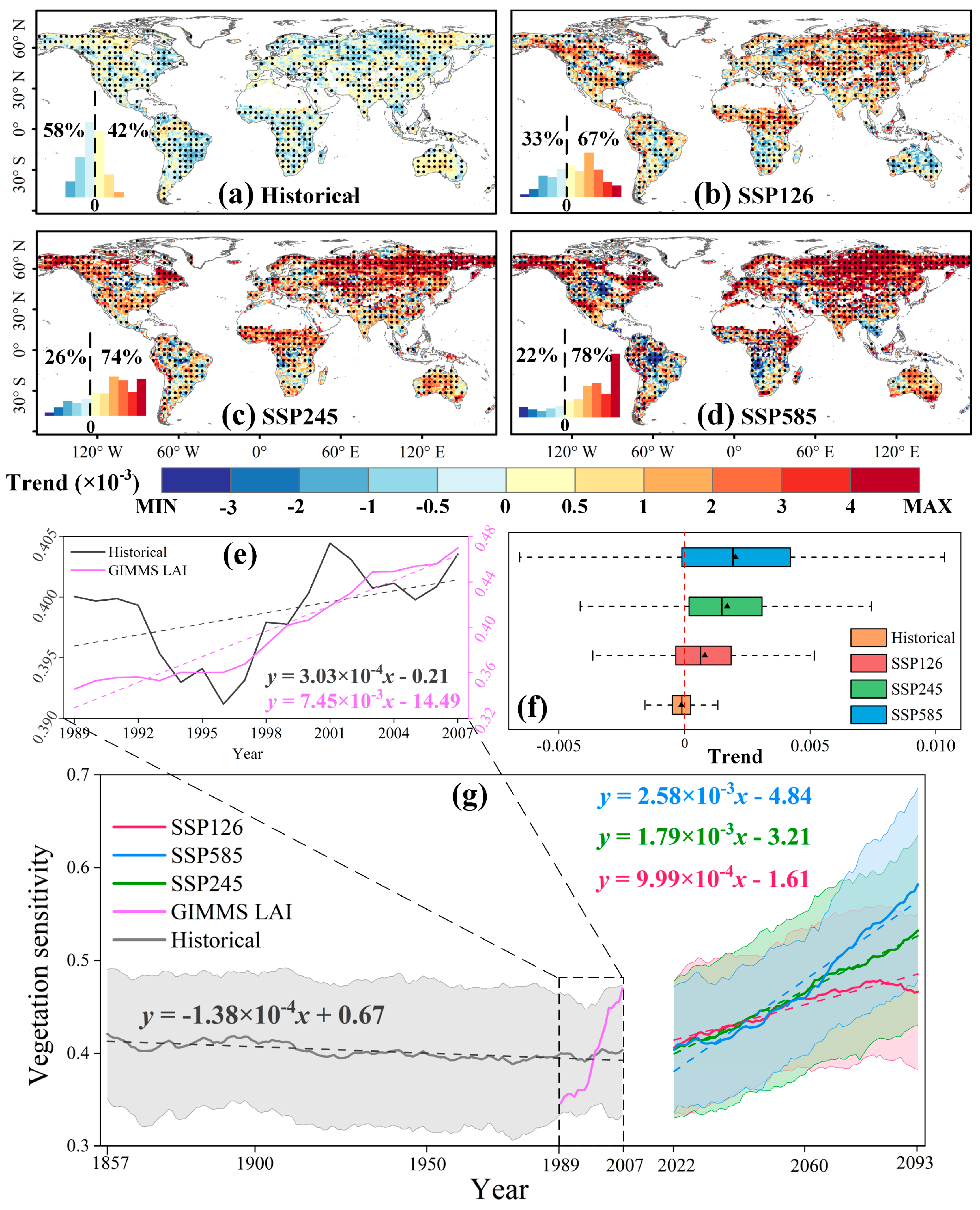
The line chart in Figure 2g shows that vegetation sensitivity in response to temperature experienced a declining trend in the historical period but exhibited an increasing trend in all the three future scenarios. The magnitudes of the increasing trends in the future period were significantly greater than that of the declining trend in the historical period. And the increasing trends gradually became larger in the order of the SSP126, SSP245, and SSP585 scenarios. Moreover, Figure 2g demonstrates that the increasing trends were similar for the SSP126, SSP245, and SSP585 scenarios, but they appeared to have contrasting trends after 2060. The increasing trend was small in SSP126 but large in SSP585. For SSP245, the increasing trend was greater than SSP126, but smaller than SSP585.
In the period from 1989 to 2007, the model- and satellite-based vegetation temperature sensitivity both showed an upward trend, illustrating that CMIP6 models well captured the temporal variability in vegetation sensitivity. Therefore, Figure 2f also demonstrates the strong robustness and reliability of our results as model- and satellite-based products provided consistent vegetation sensitivity estimates.
Overall, vegetation sensitivity showed distinguishable spatial patterns in both the historical and future periods. As shown in Figure 2a,b, the sign of trend value shifted from negative to positive in considerable pixels located in areas such as the high latitudes of Eurasia, western regions of North America, and tropical regions. The proportion of the pixels with upward trends under the SSP126 scenario significantly increased by 25% when compared with that in the historical period. For the SSP245 and SSP585 scenarios, the vegetation in tropical regions such as the Amazon and Congo forests exhibited declining sensitivity trends. In addition, Figure 2b–d jointly reveal that the proportion of pixels with an upward trend gradually increases as emission intensity rises for the SSP126 (67%), SSP245 (74%), and SSP585 (78%) scenarios, respectively.

3.2. Comparing Magnitudes of Historical and Future Vegetation Temperature Sensitivity

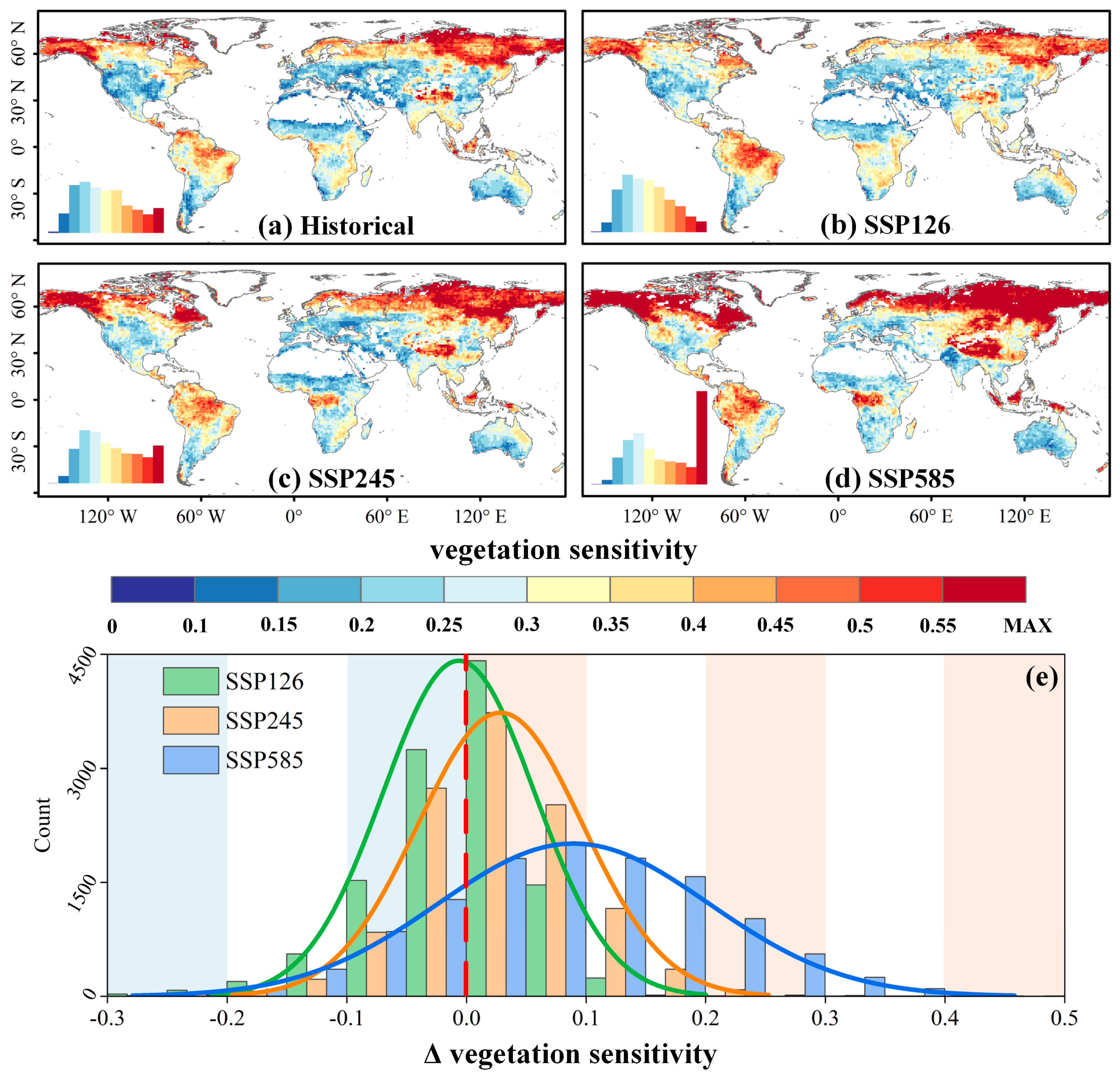
Although Figure 2 presents the spatiotemporal variability of the vegetation sensitivity in the whole investigation period, it does not clearly present the spatial distribution of vegetation temperature sensitivity under the historical and three future cases. Therefore, this section further investigates the spatial distribution of the vegetation temperature sensitivity.
As emission intensity rises, the difference values between the historical and future vegetation sensitivity gradually increase (Figure 3e). The spatial patterns of the vegetation temperature sensitivity in the historical period and the three future scenarios were similar (Figure 3a–d). Relatively high sensitivity (>0.4) was observed in high latitudes of the North Hemisphere and tropical forest areas. It is noticeable that the difference values were slightly higher in the historical period than that under the SSP126 scenario in northern Eurasia and the Tibetan Plateau. These areas, however, while under the SSP245 and SSP585 scenarios, exhibited significantly higher sensitivity compared to the historical period. In addition, vegetation temperature sensitivity in the tropical regions increased significantly under scenarios with rising carbon emissions, especially in the Congo Basin and rainforests in Southeast Asia.

3.3. Temporal Variability of the Extreme Heat Events in the 19th to 21st Centuries

The boxplots in Figure 4f illustrate that the trend in extreme heat events was generally positive and gradually became large in the three future scenarios, i.e., in the order of the SSP126, SSP245, and SSP585 scenarios. As for the historical period, the trend of the extreme heat event was significantly smaller than those in the SSP126, SSP245, and SSP585 scenarios (Figure 4f). In future projections based on the CMIP6 models, regions with relatively high trend values were concentrated in the eastern parts of North America, the Amazon rainforest, South Africa, areas near the southern Sahara Desert, Southeast Asia, and coastal regions of Australia (Figure 4b–d). In contrast, the trends in extreme heat events were relatively smaller across most tropical forests, the western and southeastern regions of Eurasia, the Great Plains, and northwestern North America. Regarding the temporal variability shown in Figure 4e, the extreme heat events increased slowly in the historical period. Nevertheless, extreme heat events increased rapidly since the 1980s. It is noticeable that SSP126 exhibited the largest increasing trend in extreme heat events before 2045, followed by the SSP245 and SSP585 scenarios. However, the situation reversed after 2045 as SSP585 exhibited the largest increasing trend, followed by the SSP245 and SSP126 scenarios.

3.4. Impact of Extreme Heat Events on Vegetation Temperature Sensitivity

In this section, we firstly explored the variability of vegetation sensitivity along with the extreme heat events. Then, the correlation between extreme heat events and vegetation temperature sensitivity was identified in the historical and future periods, respectively.
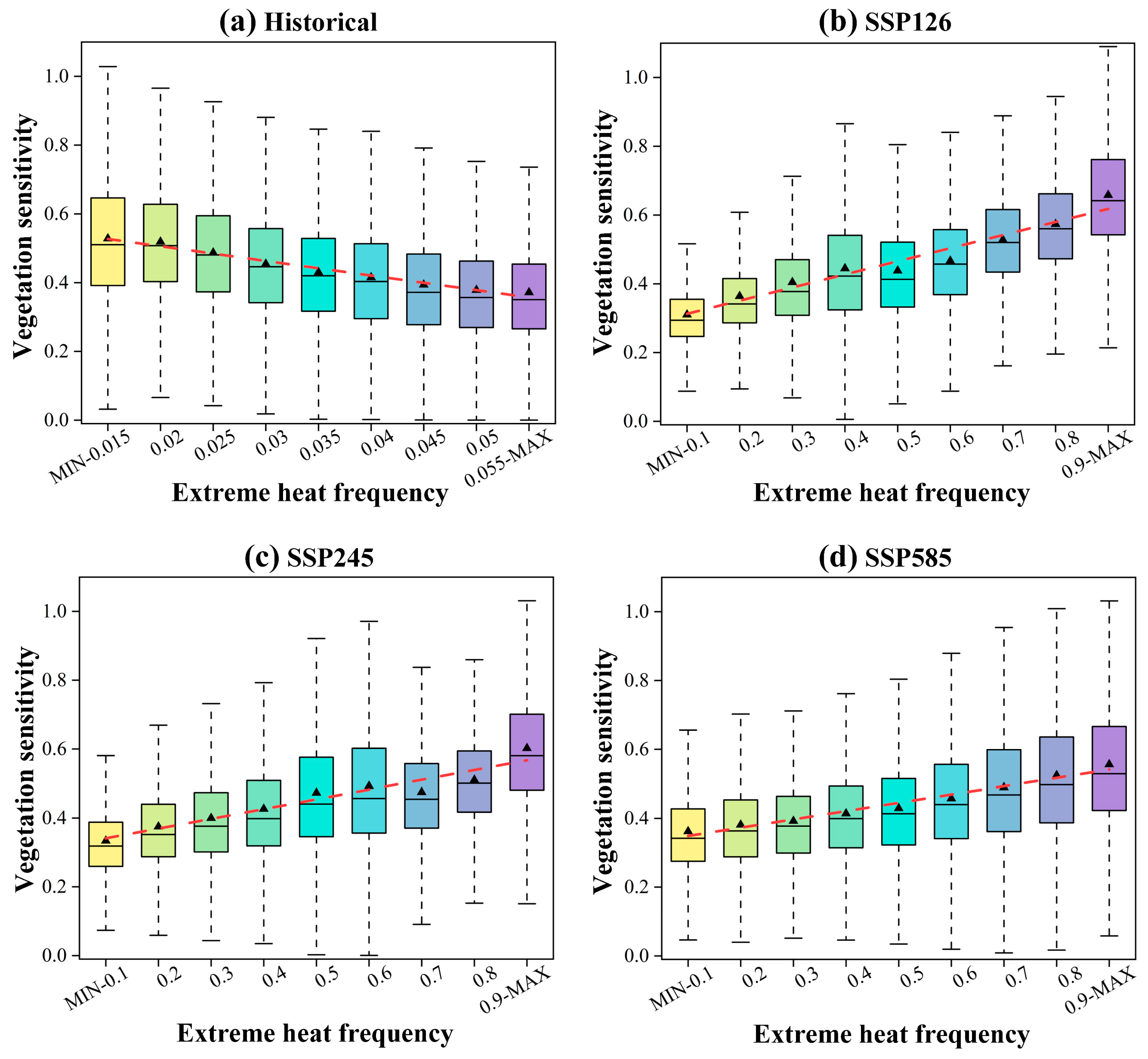
Overall, the boxplots in Figure 5 demonstrate that vegetation sensitivity exhibited a linear response to extreme heat events for all the three future scenarios. Vegetation sensitivity gradually became large as extreme heat events increased (Figure 5b–d). Nevertheless, Figure 5a shows that vegetation sensitivity appeared to decline as extreme heat events increased in the historical period, which was the opposite with respect to the three future scenarios. As illustrated in Figure 5, it is more appropriate to describe the relationship between vegetation temperature sensitivity and extreme heat events in a linear way. Based on this consideration, we explored the coupling strength between vegetation sensitivity and extreme heat frequency in Figure 6 using a linear regression method.
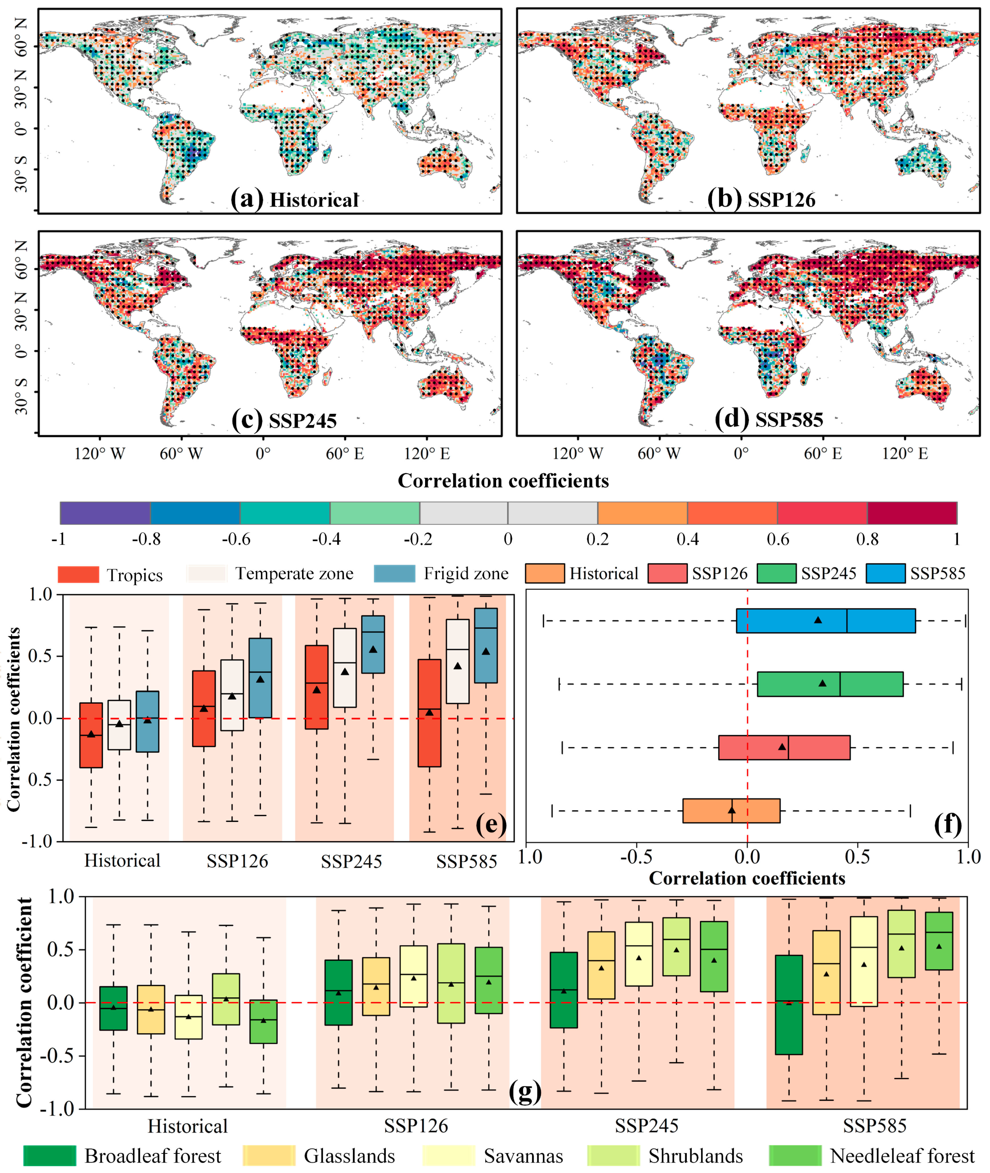
The boxplots in Figure 6f show that the correlation between vegetation temperature sensitivity and extreme heat events gradually became strong in the order of the historical, SSP126, SSP245, and SSP585 cases. In the historical period, the correlation coefficients were generally negative while they were typically positive in the three future scenarios. As shown in Figure 6e, in all four cases, the average of the correlation coefficients gradually became larger in the tropical, temperate, and frigid zones. Nevertheless, the difference of the correlation coefficients in the three climatic zones was relatively small in the historical period but large in the SSP245 and SSP585 scenarios. Comparatively, the correlation was generally strong in the frigid zone but weak in the tropics. In addition, in terms of the vegetation types, broadleaf forest regions consistently showed the weakest correlations under both the historical and three future scenarios. Spatially, the correlation was relatively strong in Brazilian highlands and part of the northern areas in Eurasia. As emission intensity increased, the correlation gradually became strong in high latitudes in the North Hemisphere for the three future scenarios (Figure 6b–d).

4. Discussion

Overall, vegetation temperature sensitivity declined in the historical period, indicating that vegetation became less responsive to temperature changes. This may be due to the fact that global warming alleviates the impact of temperature stress on vegetation in cold regions, thereby reducing the dependence of vegetation on temperature. Ref. [47] similarly noted that the response of vegetation to temperature was less pronounced during warm periods compared to cold ones. In terms of the spatial distribution of vegetation temperature sensitivity, regions with high sensitivity in the historical period were mainly located in the frigid zone, the Tibetan Plateau, and tropical forests, which is consistent with the findings of [1,42]. The frigid zone and Tibetan Plateau were characterized by cold climates and exhibited high vegetation temperature sensitivity due to the significant influence of temperature changes on plant growth in these regions [39,48]. In recent years, tropical forests were significantly impacted by both human activities and climate change. For instance, deforestation and human-induced fires have diminished the recovery capacity of tropical forests [49,50,51]. At the same time, compound extreme climate events, such as extreme heat and compound droughts, have reduced the resilience of tropical forests [52,53]. As a result, tropical forests became highly sensitive to temperature changes.
The trends in vegetation temperature sensitivity exhibited significant differences under different carbon emission intensities. Sensitivity under the SSP245 and SSP585 scenarios showed a continuous upward trend. However, the upward trend continued until around 2080 but shifted to a downward trend in the SSP126 scenario, which is consistent with the findings of [41]. Furthermore, significant differences in vegetation sensitivity to temperature among the three scenarios only emerge around 2060. This may be attributable to the differences in temperature trends in the three scenarios that are evident from around 2060 [41].
In terms of spatial distribution, the vegetation temperature sensitivity was similar in the historical and future periods. Under the SSP126 scenario, vegetation temperature sensitivity in the frigid zone and the Tibetan Plateau was significantly lower than that in the historical period. This may be attributed to the slight warming associated with the SSP126 scenario, which reduces the temperature’s limiting effect on vegetation growth in these regions [4]. Furthermore, the gradual warming associated with the SSP126 scenario may have led to adaptations in vegetation in these regions [54], resulting in lower vegetation temperature sensitivity compared to the historical period. In contrast, vegetation temperature sensitivity was generally high in the frigid zone, Tibetan Plateau, and tropical forest regions under the SSP245 and SSP585 scenarios. In these regions, the temperature under the SSP245 and SSP585 scenarios may have surpassed tolerance thresholds [7], therefore making ecosystems in the above regions highly sensitive to climate change. Additionally, high temperatures typically associate with meteorological disasters such as droughts, which exerts a compound effect on vegetation [55,56]. This diminishes the resilience and recovery capacity of ecosystems, further increasing vegetation temperature sensitivity. The results above demonstrate that high carbon emission scenarios lead to relatively high sensitivity of terrestrial ecosystems to temperature changes in cold regions and tropical forests. This underscores that the policies in the SSP126 scenario with a low carbon emission offer a sustainable development pathway that is beneficial for maintaining the stability of global terrestrial ecosystems. However, we found that the spatial patterns of the trends in vegetation temperature sensitivity exhibit relatively strong spatial heterogeneity in Figure 2a–d. Considering the spatial autocorrelation in Equation (3) may address this issue.
As carbon emission intensity increased, the impact of extreme heat events on vegetation temperature sensitivity gradually intensified. The impact of extreme heat events on vegetation temperature sensitivity was relatively low (correlation coefficient average approximately 0.2) under the SSP126 scenario and slightly higher than that in the historical period (correlation coefficient average approximately −0.1), which highlights the effectiveness of emission reduction strategies and sustainable development initiatives under the SSP126 scenario. However, in the Siberian permafrost region, the correlation between extreme heat events and vegetation temperature sensitivity was comparatively high (correlation coefficient is greater than 0.4). This indicates that vegetation in the Siberian permafrost region was particularly susceptible to the effects of extreme heat events. Previous studies showed that the tundra ecosystems in this region have low species diversity and weak resilience, making them particularly vulnerable to the extreme heat events [57]. Ref. [58] pointed out that temperatures in the permafrost regions within the Arctic Circle are currently approaching a tipping point. Continued warming may cause temperatures to exceed this tipping point, prompting the permafrost to thaw and release greenhouse gases, such as carbon dioxide and methane, that further accelerate warming [59,60]. This could lead to an increase in extreme climate events and therefore creates a vicious warming cycle in this region. In the SSP245 and SSP585 scenarios, the correlation coefficient between extreme heat events and vegetation temperature sensitivity exceeds 0.6 in the temperate zones of the Northern Hemisphere and surpasses 0.8 in the frigid regions. Our results indicate that the ecological functions of boreal forests in Russia and Canada may approach or cross critical thresholds due to the impact of extreme heat events. This may lead to a surge in carbon emissions in these regions [61]. This situation was expected to worsen under the SSP245 and SSP585 scenarios with relatively high carbon emissions. We argue that more attention should be paid to Russia and Canada due to the large areas of taiga forests, such as by making policies to strictly control human-induced carbon emissions to cope with the intensified global warming situation. Additionally, the IPCC Sixth Assessment Report highlighted that achieving sustainable carbon emission strategies is challenging [62]. Even if energy-saving and emission reduction policies under the SSP126 scenario were followed, future warming may still exceed the 2 °C target set by the Paris Agreement. Therefore, we suggest considering extreme heat events in the carbon cycle studies in the future.
This study has several limitations. Firstly, various definitions of extreme heat have been proposed based on region, vegetation type, and environmental factors [3,63], which may influence the identification of extreme heat events in our experiment. Secondly, CMIP6 models have uncertainties. Due to significant deviations in the simulated trend magnitude and the temporal pattern of interannual variability, most CMIP6 models failed to capture the temporal variability of annual LAI effectively [21]. Ref. [64] highlighted considerable uncertainty in the CMIP6 models regarding the simulation of extreme climate events. The data used for bias correction also have uncertainties. The resampling of remote sensing data from 0.1° × 0.1° to 1° × 1° grids resulted in unavoidable information loss. Then, the short length of the GIMMS LAI4g and ERA5 data (2015–2020) used for the bias correction in the future period would also introduce inevitable uncertainties. Also, the effectiveness of the bias correction for the future period in our work may be significantly influenced by the baseline data with a relatively short period (2015–2020). Finally, wildfires may affect the temperature sensitivity of vegetation. However, this factor was not considered in our analysis as [65] reported a severe deficiency of the CMIP6 models to simulate wildfire risk regarding its seasonal variations.

5. Conclusions

This study utilized LAI and average temperature data from CMIP6 to investigate the spatiotemporal variability of vegetation temperature sensitivity from the 19th to the 21st century, as well as the impact of extreme heat events on vegetation temperature sensitivity under different carbon emission intensity scenarios. The main conclusions are as follows:
(1)
Overall, vegetation temperature sensitivity showed a declining trend in the historical period. The sensitivity trends under different future carbon emission scenarios exhibited significant differences. The sensitivity exhibited an upward trend until 2080 but yielded a declining trend after 2080 under the SSP126 scenario. In contrast, vegetation temperature sensitivity continuously increased under the SSP245 and SSP585 scenarios.
(2)
Vegetation temperature sensitivity gradually increased as carbon emission intensity rose. Specifically, the historical period exhibited the smallest sensitivity, followed by SSP126, SSP245, and SSP585. High sensitivity values were distributed in the high latitudes of the Northern Hemisphere, the Tibetan Plateau, and tropical forests for both the historical and future periods. Sensitivity in the high latitudes of the Northern Hemisphere and the Tibetan Plateau was lower under the SSP126 scenario than that in the historical period. However, the sensitivity of tropical forests was higher than that in the historical period in all three future scenarios.
(3)
Extreme heat events were linearly correlated with vegetation temperature sensitivity, and their correlation became strong as carbon emission intensity increased. During the historical period, the impact of the extreme heat events on vegetation temperature sensitivity was generally weak as the average of the associated correlation coefficients was approximately -0.1. Under the SSP126 scenario, the correlation between extreme heat events and vegetation temperature sensitivity in the Arctic permafrost region was relatively strong (correlation coefficient greater than 0.4). As for the SSP245 and SSP585 scenarios, the correlation was strong in the temperate and frigid zones (correlation coefficient greater than 0.6).

Author Contributions

K.W. conceived the ideas for this research. H.Y. and C.Z. designed the research and wrote the draft. T.J., J.C., Z.Z. and Z.H. collected and processed the data. All authors have read and agreed to the published version of the manuscript.

Funding

This research was funded by the Hainan Provincial Natural Science Foundation of China (623RC447, 423MS117, NHXXRCXM202352), the Hainan University start-up fund (KYQD(ZR)22084), the National Natural Science Foundation of China (Grant No. U23A2002), and the Second Tibetan Plateau Scientific Expedition and Research Program (Grant NO. 2019QZKK0405).

Data Availability Statement

The data used are primarily reflected in the article. Other relevant data are available from the corresponding author upon request.

Conflicts of Interest

The authors declare that they have no known competing financial interests or personal relationships that could have appeared to influence the work reported in this paper.

References

  1. Chen, J.; Yang, H.; Jin, T.; Wu, K. Assessment of Terrestrial Ecosystem Sensitivity to Climate Change in Arid, Semi-Arid, Sub-Humid, and Humid Regions Using EVI, LAI, and SIF Products. Ecol. Indic. 2024, 158, 111511. [Google Scholar] [CrossRef]
  2. Li, D.; Wu, S.; Liu, L.; Zhang, Y.; Li, S. Vulnerability of the Global Terrestrial Ecosystems to Climate Change. Glob. Chang. Biol. 2018, 24, 4095–4106. [Google Scholar] [CrossRef] [PubMed]
  3. Horton, R.M.; Mankin, J.S.; Lesk, C.; Coffel, E.; Raymond, C. A Review of Recent Advances in Research on Extreme Heat Events. Curr. Clim. Chang. Rep. 2016, 2, 242–259. [Google Scholar] [CrossRef]
  4. Liu, D.; Zhang, J.; Zhao, L.; Zhao, S.; Cui, G. The Positive Impact of Extreme Heat on Vegetation Growth in Northeast Asia. Agric. For. Meteorol. 2024, 347, 109918. [Google Scholar] [CrossRef]
  5. Baumbach, L.; Siegmund, J.F.; Mittermeier, M.; Donner, R.V. Impacts of Temperature Extremes on European Vegetation during the Growing Season. Biogeosciences 2017, 14, 4891–4903. [Google Scholar] [CrossRef]
  6. Bennett, A.C.; Rodrigues de Sousa, T.; Monteagudo-Mendoza, A.; Esquivel-Muelbert, A.; Morandi, P.S.; Coelho de Souza, F.; Castro, W.; Duque, L.F.; Flores Llampazo, G.; Manoel dos Santos, R.; et al. Sensitivity of South American Tropical Forests to an Extreme Climate Anomaly. Nat. Clim. Change 2023, 13, 967–974. [Google Scholar] [CrossRef]
  7. Doughty, C.E.; Keany, J.M.; Wiebe, B.C.; Rey-Sanchez, C.; Carter, K.R.; Middleby, K.B.; Cheesman, A.W.; Goulden, M.L.; Da Rocha, H.R.; Miller, S.D.; et al. Tropical Forests Are Approaching Critical Temperature Thresholds. Nature 2023, 621, 105–111. [Google Scholar] [CrossRef]
  8. Zhu, B.; Cheng, Y.; Hu, X.; Chai, Y.; Berghuijs, W.R.; Borthwick, A.G.L.; Slater, L. Constrained Tropical Land Temperature-Precipitation Sensitivity Reveals Decreasing Evapotranspiration and Faster Vegetation Greening in CMIP6 Projections. npj Clim. Atmos. Sci. 2023, 6, 91. [Google Scholar] [CrossRef]
  9. Bastos, A.; Gouveia, C.M.; Trigo, R.M.; Running, S.W. Analysing the Spatio-Temporal Impacts of the 2003 and 2010 Extreme Heatwaves on Plant Productivity in Europe. Biogeosciences 2014, 11, 3421–3435. [Google Scholar] [CrossRef]
  10. Alemayehu, T.; van Griensven, A.; Woldegiorgis, B.T.; Bauwens, W. An Improved SWAT Vegetation Growth Module and Its Evaluation for Four Tropical Ecosystems. Hydrol. Earth Syst. Sci. 2017, 21, 4449–4467. [Google Scholar] [CrossRef]
  11. Cox, P.M.; Pearson, D.; Booth, B.B.; Friedlingstein, P.; Huntingford, C.; Jones, C.D.; Luke, C.M. Sensitivity of Tropical Carbon to Climate Change Constrained by Carbon Dioxide Variability. Nature 2013, 494, 341–344. [Google Scholar] [CrossRef] [PubMed]
  12. Wu, X.; Liu, H.; Li, X.; Piao, S.; Ciais, P.; Guo, W.; Yin, Y.; Poulter, B.; Peng, C.; Viovy, N.; et al. Higher Temperature Variability Reduces Temperature Sensitivity of Vegetation Growth in Northern Hemisphere. Geophys. Res. Lett. 2017, 44, 6173–6181. [Google Scholar] [CrossRef]
  13. Gao, S.; Liang, E.; Liu, R.; Babst, F.; Camarero, J.J.; Fu, Y.H.; Piao, S.; Rossi, S.; Shen, M.; Wang, T.; et al. An Earlier Start of the Thermal Growing Season Enhances Tree Growth in Cold Humid Areas but Not in Dry Areas. Nat. Ecol. Evol. 2022, 6, 397–404. [Google Scholar] [CrossRef] [PubMed]
  14. Xiong, T.; Du, S.; Zhang, H.; Zhang, X. Satellite Observed Reversal in Trends of Spring Phenology in the Middle-High Latitudes of the Northern Hemisphere during the Global Warming Hiatus. Glob. Chang. Biol. 2023, 29, 2227–2241. [Google Scholar] [CrossRef]
  15. Zhang, Y.; Hong, S.; Liu, D.; Piao, S. Susceptibility of Vegetation Low-Growth to Climate Extremes on Tibetan Plateau. Agric. For. Meteorol. 2023, 331, 109323. [Google Scholar] [CrossRef]
  16. Berdugo, M.; Delgado-Baquerizo, M.; Soliveres, S.; Hernández-Clemente, R.; Zhao, Y.; Gaitán, J.J.; Gross, N.; Saiz, H.; Maire, V.; Lehman, A.; et al. Global Ecosystem Thresholds Driven by Aridity. Science 2020, 367, 787–790. [Google Scholar] [CrossRef]
  17. Sun, B.; Jiang, M.; Han, G.; Zhang, L.; Zhou, J.; Bian, C.; Du, Y.; Yan, L.; Xia, J. Experimental Warming Reduces Ecosystem Resistance and Resilience to Severe Flooding in a Wetland. Sci. Adv. 2022, 8, eabl9526. [Google Scholar] [CrossRef] [PubMed]
  18. Wigneron, J.P.; Fan, L.; Ciais, P.; Bastos, A.; Brandt, M.; Chave, J.; Saatchi, S.; Baccini, A.; Fensholt, R. Tropical Forests Did Not Recover from the Strong 2015–2016 El Niño Event. Sci. Adv. 2020, 6, eaay4603. [Google Scholar] [CrossRef]
  19. De Keersmaecker, W.; Lhermitte, S.; Tits, L.; Honnay, O.; Somers, B.; Coppin, P. A Model Quantifying Global Vegetation Resistance and Resilience to Short-Term Climate Anomalies and Their Relationship with Vegetation Cover. Glob. Ecol. Biogeogr. 2015, 24, 539–548. [Google Scholar] [CrossRef]
  20. Wu, K.; Ryu, D.; Nie, L.; Shu, H. Time-Variant Error Characterization of SMAP and ASCAT Soil Moisture Using Triple Collocation Analysis. Remote Sens. Environ. 2021, 256, 112324. [Google Scholar] [CrossRef]
  21. Song, X.; Wang, D.Y.; Li, F.; Zeng, X.D. Evaluating the Performance of CMIP6 Earth System Models in Simulating Global Vegetation Structure and Distribution. Adv. Clim. Chang. Res. 2021, 12, 584–595. [Google Scholar] [CrossRef]
  22. Piao, S.; Nan, H.; Huntingford, C.; Ciais, P.; Friedlingstein, P.; Sitch, S.; Peng, S.; Ahlström, A.; Canadell, J.G.; Cong, N.; et al. Evidence for a Weakening Relationship between Interannual Temperature Variability and Northern Vegetation Activity. Nat. Commun. 2014, 5, 5018. [Google Scholar] [CrossRef] [PubMed]
  23. Eyring, V.; Bony, S.; Meehl, G.A.; Senior, C.A.; Stevens, B.; Stouffer, R.J.; Taylor, K.E. Overview of the Coupled Model Intercomparison Project Phase 6 (CMIP6) Experimental Design and Organization. Geosci. Model Dev. 2016, 9, 1937–1958. [Google Scholar] [CrossRef]
  24. Ziehn, T.; Chamberlain, M.A.; Law, R.M.; Lenton, A.; Bodman, R.W.; Dix, M.; Stevens, L.; Wang, Y.P.; Srbinovsky, J. The Australian Earth System Model: ACCESS-ESM1.5. J. South. Hemisph. Earth Syst. Sci. 2020, 70, 193–214. [Google Scholar] [CrossRef]
  25. Wu, T.; Lu, Y.; Fang, Y.; Xin, X.; Li, L.; Li, W.; Jie, W.; Zhang, J.; Liu, Y.; Zhang, L.; et al. The Beijing Climate Center Climate System Model (BCC-CSM): The Main Progress from CMIP5 to CMIP6. Geosci. Model Dev. 2019, 12, 1573–1600. [Google Scholar] [CrossRef]
  26. Swart, N.; Cole, J.; Kharin, V.; Lazare, M.; Scinocca, J.; Gillett, N.; Anstey, J.; Arora, V.; Christian, J.; Hanna, S.; et al. The Canadian Earth System Model Version 5 (CanESM5.0.3). Geosci. Model Dev. 2019, 12, 4823–4873. [Google Scholar] [CrossRef]
  27. Cherchi, A.; Fogli, P.G.; Lovato, T.; Peano, D.; Iovino, D.; Gualdi, S.; Masina, S.; Scoccimarro, E.; Materia, S.; Bellucci, A.; et al. Global Mean Climate and Main Patterns of Variability in the CMCC-CM2 Coupled Model. J. Adv. Model. Earth Syst. 2019, 11, 185–209. [Google Scholar] [CrossRef]
  28. Volodin, E. The Mechanisms of Cloudiness Evolution Responsible for Equilibrium Climate Sensitivity in Climate Model INM-CM4-8. Geophys. Res. Lett. 2021, 48, e2021GL096204. [Google Scholar] [CrossRef]
  29. Volodin, E.M.; Mortikov, E.V.; Kostrykin, S.V.; Galin, V.Y.; Lykossov, V.N.; Gritsun, A.S.; Diansky, N.A.; Gusev, A.V.; Iakovlev, N.G. Simulation of the Present-Day Climate with the Climate Model INMCM5. Clim. Dyn. 2017, 49, 3715–3734. [Google Scholar] [CrossRef]
  30. Boucher, O.; Servonnat, J.; Albright, A.L.; Aumont, O.; Balkanski, Y.; Bastrikov, V.; Bekki, S.; Bonnet, R.; Bony, S.; Bopp, L.; et al. Presentation and Evaluation of the IPSL-CM6A-LR Climate Model. J. Adv. Model. Earth Syst. 2020, 12, e2019MS002010. [Google Scholar] [CrossRef]
  31. Held, I.M.; Guo, H.; Adcroft, A.; Dunne, J.P.; Horowitz, L.W.; Krasting, J.; Shevliakova, E.; Winton, M.; Zhao, M.; Bushuk, M.; et al. Structure and Performance of GFDL’s CM4.0 Climate Model. J. Adv. Model. Earth Syst. 2019, 11, 3691–3727. [Google Scholar] [CrossRef]
  32. Mauritsen, T.; Bader, J.; Becker, T.; Behrens, J.; Bittner, M.; Brokopf, R.; Brovkin, V.; Claussen, M.; Crueger, T.; Esch, M.; et al. Developments in the MPI-M Earth System Model Version 1.2 (MPI-ESM1.2) and Its Response to Increasing CO2. J. Adv. Model. Earth Syst. 2019, 11, 998–1038. [Google Scholar] [CrossRef] [PubMed]
  33. Räty, O.; Räisänen, J.; Ylhäisi, J.S. Evaluation of Delta Change and Bias Correction Methods for Future Daily Precipitation: Intermodel Cross-Validation Using ENSEMBLES Simulations. Clim. Dyn. 2014, 42, 2287–2303. [Google Scholar] [CrossRef]
  34. Jose, D.M.; Dwarakish, G.S. Bias Correction and Trend Analysis of Temperature Data by a High-Resolution CMIP6 Model over a Tropical River Basin. Asia-Pac. J. Atmos. Sci. 2022, 58, 97–115. [Google Scholar] [CrossRef]
  35. Chen, J.; Yang, Y.; Tang, J. Bias Correction of Surface Air Temperature and Precipitation in CORDEX East Asia Simulation: What Should We Do When Applying Bias Correction? Atmos. Res. 2022, 280, 106439. [Google Scholar] [CrossRef]
  36. Beyer, R.; Krapp, M.; Manica, A. An Empirical Evaluation of Bias Correction Methods for Palaeoclimate Simulations. Clim. Past 2020, 16, 1493–1508. [Google Scholar] [CrossRef]
  37. Wu, K.; Ryu, D.; Wagner, W.; Hu, Z. A Global-Scale Intercomparison of Triple Collocation Analysis- and Ground-Based Soil Moisture Time-Variant Errors Derived from Different Rescaling Techniques. Remote Sens. Environ. 2023, 285, 113387. [Google Scholar] [CrossRef]
  38. Cao, S.; Li, M.; Zhu, Z.; Wang, Z.; Zha, J.; Zhao, W.; Duanmu, Z.; Chen, J.; Zheng, Y.; Chen, Y.; et al. Spatiotemporally Consistent Global Dataset of the GIMMS Leaf Area Index (GIMMS LAI4g) from 1982 to 2020. Earth Syst. Sci. Data 2023, 15, 4877–4899. [Google Scholar] [CrossRef]
  39. Wu, K.; Chen, J.; Yang, H.; Yang, Y.; Hu, Z. Spatiotemporal Variations in the Sensitivity of Vegetation Growth to Typical Climate Factors on the Qinghai–Tibet Plateau. Remote Sens. 2023, 15, 2355. [Google Scholar] [CrossRef]
  40. Shen, M.; Zhu, X.; Peng, D.; Jiang, N.; Huang, Y.; Chen, J.; Wang, C.; Zhao, W. Greater Temperature Sensitivity of Vegetation Greenup Onset Date in Areas with Weaker Temperature Seasonality across the Northern Hemisphere. Agric. For. Meteorol. 2022, 313, 108759. [Google Scholar] [CrossRef]
  41. Wang, Y.; Peng, L.; Yue, Y.; Chen, T. Global Vegetation-Temperature Sensitivity and Its Driving Forces in the 21st Century. Earth’s Future 2024, 12, e2022EF003395. [Google Scholar] [CrossRef]
  42. Seddon, A.W.R.; Macias-Fauria, M.; Long, P.R.; Benz, D.; Willis, K.J. Sensitivity of Global Terrestrial Ecosystems to Climate Variability. Nature 2016, 531, 229–232. [Google Scholar] [CrossRef]
  43. Lahiri, S.N. On the Moving Block Bootstrap under Long Range Dependence. Stat. Probab. Lett. 1993, 18, 405–413. [Google Scholar] [CrossRef]
  44. Kendall, M.G. Rank Correlation Methods; Griffin: Oxford, UK, 1948. [Google Scholar]
  45. Mann, H.B. Nonparametric Tests Against Trend. Econometrica 1945, 13, 245–259. [Google Scholar] [CrossRef]
  46. Yang, Q.; Jiang, C.; Ding, T. Impacts of Extreme-High-Temperature Events on Vegetation in North China. Remote Sens. 2023, 15, 4542. [Google Scholar] [CrossRef]
  47. Wang, C.; Cao, R.; Chen, J.; Rao, Y.; Tang, Y. Temperature Sensitivity of Spring Vegetation Phenology Correlates to Within-Spring Warming Speed over the Northern Hemisphere. Ecol. Indic. 2015, 50, 62–68. [Google Scholar] [CrossRef]
  48. Piao, S.; Cui, M.; Chen, A.; Wang, X.; Ciais, P.; Liu, J.; Tang, Y. Altitude and Temperature Dependence of Change in the Spring Vegetation Green-up Date from 1982 to 2006 in the Qinghai-Xizang Plateau. Agric. For. Meteorol. 2011, 151, 1599–1608. [Google Scholar] [CrossRef]
  49. Boulton, C.A.; Lenton, T.M.; Boers, N. Pronounced Loss of Amazon Rainforest Resilience since the Early 2000s. Nat. Clim. Chang. 2022, 12, 271–278. [Google Scholar] [CrossRef]
  50. Lovejoy, T.E.; Nobre, C. Amazon Tipping Point: Last Chance for Action. Sci. Adv. 2019, 5, eaba2949. [Google Scholar] [CrossRef]
  51. Flores, B.M.; Staal, A.; Jakovac, C.C.; Hirota, M.; Holmgren, M.; Oliveira, R.S. Soil Erosion as a Resilience Drain in Disturbed Tropical Forests. Plant Soil 2020, 450, 11–25. [Google Scholar] [CrossRef]
  52. Mukherjee, S.; Mishra, A.K. Increase in Compound Drought and Heatwaves in a Warming World. Geophys. Res. Lett. 2021, 48, e2020GL090617. [Google Scholar] [CrossRef]
  53. Zhou, S.; Wu, S.; Gao, J.; Liu, L.; Li, D.; Yan, R.; Wang, J. Increased Stress from Compound Drought and Heat Events on Vegetation. Sci. Total Environ. 2024, 949, 175113. [Google Scholar] [CrossRef] [PubMed]
  54. Lu, C.; van Groenigen, K.J.; Gillespie, M.A.K.; Hollister, R.D.; Post, E.; Cooper, E.J.; Welker, J.M.; Huang, Y.; Min, X.; Chen, J.; et al. Diminishing Warming Effects on Plant Phenology over Time. New Phytol. 2024; Early View. [Google Scholar] [CrossRef]
  55. Hao, Z.; Hao, F.; Xia, Y.; Feng, S.; Sun, C.; Zhang, X.; Fu, Y.; Hao, Y.; Zhang, Y.; Meng, Y. Compound Droughts and Hot Extremes: Characteristics, Drivers, Changes, and Impacts. Earth-Sci. Rev. 2022, 235, 104241. [Google Scholar] [CrossRef]
  56. Zhang, L.; Yu, X.; Zhou, T.; Zhang, W.; Hu, S.; Clark, R. Understanding and Attribution of Extreme Heat and Drought Events in 2022: Current Situation and Future Challenges. Adv. Atmos. Sci. 2023, 40, 1941–1951. [Google Scholar] [CrossRef]
  57. Dobricic, S.; Russo, S.; Pozzoli, L.; Wilson, J.; Vignati, E. Increasing Occurrence of Heat Waves in the Terrestrial Arctic. Environ. Res. Lett. 2020, 15, 024022. [Google Scholar] [CrossRef]
  58. Lenton, T.M.; Rockström, J.; Gaffney, O.; Rahmstorf, S.; Richardson, K.; Steffen, W.; Schellnhuber, H.J. Climate Tipping Points—Too Risky to Bet Against. Nature 2019, 575, 592–595. [Google Scholar] [CrossRef] [PubMed]
  59. See, C.R.; Virkkala, A.-M.; Natali, S.M.; Rogers, B.M.; Mauritz, M.; Biasi, C.; Bokhorst, S.; Boike, J.; Bret-Harte, M.S.; Celis, G.; et al. Decadal Increases in Carbon Uptake Offset by Respiratory Losses across Northern Permafrost Ecosystems. Nat. Clim. Chang. 2024, 14, 853–862. [Google Scholar] [CrossRef]
  60. Walker, X.J.; Baltzer, J.L.; Cumming, S.G.; Day, N.J.; Ebert, C.; Goetz, S.; Johnstone, J.F.; Potter, S.; Rogers, B.M.; Schuur, E.A.G.; et al. Increasing Wildfires Threaten Historic Carbon Sink of Boreal Forest Soils. Nature 2019, 572, 520–523. [Google Scholar] [CrossRef]
  61. Liang, L.; Liang, S.; Zeng, Z. Extreme Climate Sparks Record Boreal Wildfires and Carbon Surge in 2023. Innovation 2024, 5, 100631. [Google Scholar] [CrossRef]
  62. DeAngelo, J.; Azevedo, I.; Bistline, J.; Clarke, L.; Luderer, G.; Byers, E.; Davis, S.J. Energy Systems in Scenarios at Net-Zero CO2 Emissions. Nat. Commun. 2021, 12, 6096. [Google Scholar] [CrossRef]
  63. Perkins, S.E. A Review on the Scientific Understanding of Heatwaves—Their Measurement, Driving Mechanisms, and Changes at the Global Scale. Atmos. Res. 2015, 164–165, 242–267. [Google Scholar] [CrossRef]
  64. Chen, H.; Sun, J.; Lin, W.; Xu, H. Comparison of CMIP6 and CMIP5 Models in Simulating Climate Extremes. Sci. Bull. 2020, 65, 1415–1418. [Google Scholar] [CrossRef] [PubMed]
  65. Gallo, C.; Eden, J.M.; Dieppois, B.; Drobyshev, I.; Fulé, P.Z.; San-Miguel-Ayanz, J.; Blackett, M. Evaluation of CMIP6 Model Performances in Simulating Fire Weather Spatiotemporal Variability on Global and Regional Scales. Geosci. Model Dev. 2023, 16, 3103–3122. [Google Scholar] [CrossRef]
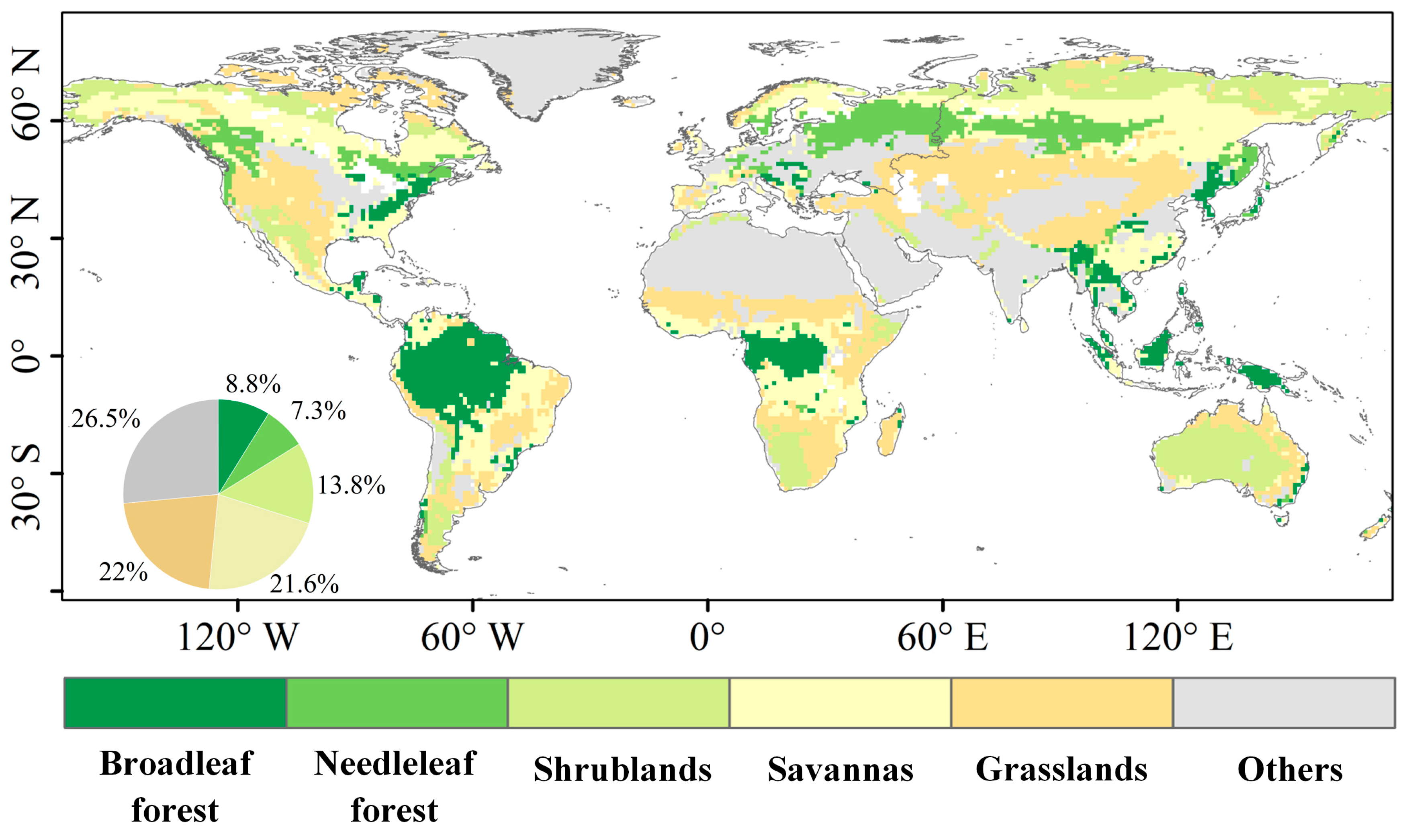
Figure 1. Spatial distribution of the vegetation types considered in our work.
Remotesensing 16 03708 g001
Figure 2. Spatial patterns of the trend in vegetation temperature sensitivity in (a) historical and future periods under the (b) SSP126, (c) SSP245, and (d) SSP585 scenarios. The black dots denote the trend values that passed the significance test (p < 0.05) in the overlying regions. Proportions of the significant pixels in a-d are 0.64, 0.65, 0.75, and 0.80, respectively. (e) compares the temporal variability of spatially averaged model- and satellite-based vegetation sensitivity from 1989 to 2007. (f) provides the boxplots of trend values illustrated in (ad). (g) shows the temporal variability of spatially averaged model- and satellite-based vegetation sensitivity from 1857 to 2093. The shaded areas in (g) describe the vegetation sensitivity uncertainty, that is, the variance of vegetation sensitivity derived from the 10 CMIP6 models.
Remotesensing 16 03708 g002
Figure 3. Spatial distribution of vegetation temperature sensitivity in the (a) historical and future periods under the (b) SSP126, (c) SSP245, and (d) SSP585 scenarios, respectively. (e) describes histograms of the difference values between future and historical vegetation temperature sensitivity (future sensitivity minus historical sensitivity).
Remotesensing 16 03708 g003
Figure 4. Spatial patterns of trend in extreme heat events in the (a) historical and future periods under the (b) SSP126, (c) SSP245, and (d) SSP585 scenarios. The black dots denote the trend values that passed the significance test (p < 0.05) in the overlying regions. Nearly all pixels in subfigures (ad) passed the significance test. (f) describes the corresponding boxplots for the trend values illustrated in (ad). (e) presents the temporal variability of the spatially averaged extreme heat events for the above four cases.
Remotesensing 16 03708 g004
Figure 5. Variations of the vegetation sensitivity along with the extreme heat events for the (a) historical and (b) SSP126, (c) SSP245, and (d) SSP585 scenarios. The extreme heat events were classified into 9 intervals and the associated vegetation sensitivity values were gleaned for each of the intervals.
Remotesensing 16 03708 g005
Figure 6. Spatial patterns of the correlation coefficients between vegetation temperature sensitivity and extreme heat events in the (a) historical and (bd) future scenarios. The black dots denote the trend values that passed the significance test (p < 0.05) in the overlying regions. Proportions of significant pixels in (ad) are 0.62, 0.64, 0.75, and 0.81, respectively. (f) describes the box plots of correlation coefficients shown in (ad), while (e,g) further investigate the correlation coefficients categorized by different temperature zones and vegetation types.
Remotesensing 16 03708 g006
Table 1. A summary of the 10 CMIP6 models used in our work.
ModelsInstituteSpatial ResolutionReferences
ACCESS-ESM1-5CSIRO, Australia1.875° × 1.241°[24]
BCC-CSM2-MRBCC, China1.125° × 1.125°[25]
CanESM5CCCma, Canada2.8125° × 2.8125°[26]
CMCC-ESM2CMCC, Italy0.9° × 1.25°[27]
INM-CM4-8INM, Russia2° × 1.5°[28]
INM-CM5-0INM, Russia2° × 1.5°[29]
IPSL-CM6A-LRIPSL, France2.5° × 1.259°[30]
GFDL-ESM4GFDL, USA1.3°  ×  1°[31]
MPI-ESM1-2-HRDKRZ, Germany1.875° × 1.875°[32]
MPI-ESM1-2-LRMPI-M, Germany2.5° × 1.875°[32]
Disclaimer/Publisher’s Note: The statements, opinions and data contained in all publications are solely those of the individual author(s) and contributor(s) and not of MDPI and/or the editor(s). MDPI and/or the editor(s) disclaim responsibility for any injury to people or property resulting from any ideas, methods, instructions or products referred to in the content.