Technical Note

A Fast and Robust Range Alignment Method for ISAR Imaging Based on a Deep Learning Network and Regional Multi-Scale Minimum Entropy Method

by
Qianhao Ning
,
Hongyuan Wang
,
Zhiqiang Yan
*,
Zijian Wang
and
Yinxi Lu
Space Optical Engineering Research Center, Harbin Institute of Technology, Harbin 150001, China
*
Author to whom correspondence should be addressed.
Remote Sens. 2024, 16(19), 3677; https://doi.org/10.3390/rs16193677
Submission received: 14 August 2024 / Revised: 25 September 2024 / Accepted: 29 September 2024 / Published: 2 October 2024

Abstract

:
In inverse synthetic aperture radar (ISAR) imaging, range alignment (RA) is crucial for translational compensation. To address the need for rapidity and accuracy in the RA process, a fast and robust range alignment method is proposed based on a deep learning network and minimum entropy (ME) method. The proposed method consists primarily of two components: the CNN-RNN attention mechanism network (CRAN) architecture and the regional multi-scale minimum entropy (RMSME) method. The main distinction of this method from existing approaches lies in its utilization of a deep learning network for rapid coarse alignment, followed by the search for minimum entropy within local regions at multiple scales. The integration strategy effectively addresses the current challenges of poor generalization in deep learning networks and low efficiency in the traditional ME method. The experimental results of simulation data indicate that the proposed method achieves the best range alignment performance compared to RNN, CRAN, and the traditional ME method. The experimental results of the measured data further validate the practicality of the proposed method. This research provides reference significance for the joint application of deep learning and traditional methods in the RA process.

1. Introduction

Inverse synthetic aperture radar (ISAR) imaging is a crucial technique for achieving high-resolution radar imaging. Its range resolution is primarily attributed to the bandwidth, while the cross-range resolution is derived from the relative motion between the target and the radar. However, uncertain relative motion also leads to the need for motion compensation in the imaging process of ISAR. Translational compensation in motion compensation usually includes range alignment (RA) and phase correction. The echoes after range compression at different slow times exhibit offsets in the range dimension due to relative motion. The core challenge addressed by range alignment techniques is how to compensate for these offsets, ensuring that signals from the same scatter point at different slow times align within the same range cell. The quality of range alignment directly influences the difficulty of subsequent phase correction and the final focusing accuracy in ISAR imaging. Therefore, research on range alignment methods has consistently garnered attention from researchers in relevant fields.
Traditional approaches attempt to compensate for every offset in range profiles (RP), aiming to optimize a specific evaluation metric. Two common traditional methods are the cross-correlation method and the minimum entropy (ME) method [1,2]. The cross-correlation method involves finding the maximum value of the correlation function, while the minimum entropy method seeks to minimize the entropy function. Due to its superior compensation accuracy, the minimum entropy method has been widely employed and has evolved in its application. Currently, there are many minimum entropy methods with targeted enhancements [3,4,5,6,7]. In 2009, a method to improve efficiency by minimizing the average range profile (ARP) of entropy was proposed [3]. In 2013, scholars proposed a coordinate descent algorithm to solve the optimization problem implemented by the quasi-Newton algorithm and improved the entropy minimization method under a low signal-to-noise ratio [4]. In 2015, scholars proposed a fast MEA method based on Newton’s method to improve computational efficiency [5]. In 2016, scholars used local quadratic curves to approximate the minimum entropy to improve accuracy [6]. In 2018, a more robust minimum entropy method was proposed by finding the Doppler centroid [7]. Some parameterized methods can effectively estimate motion parameters under stable imaging conditions [8,9,10,11,12]. In 2019, a noise-robust compensation method was proposed that used tracking information and parameter minimum entropy optimization to compensate for the 2-D spatial-variant phase errors of the maneuvering target [8]. In 2021, scholars proposed a translational motion compensation method based on parabolic curve detection and entropy minimization in spaceborne ISAR imagery for space targets [9]. In 2022, a noise-robust high-speed motion compensation algorithm was proposed using the continuity of a high-speed moving target’s velocity [10]. In 2022, scholars proposed an improved parametric translational motion compensation algorithm based on signal phase order reduction (SPOR) and minimum entropy [11]. In 2022, scholars proposed a noise-robust translational motion compensation method based on high-order local polynomial transform-generalized scaled Fourier transform (HLPT-GSCFT) [12]. However, the prerequisite for achieving high precision with most traditional minimum entropy methods is to iterate every offset to compute entropy values, leading to time-consuming and inefficient processes. With the rapid development of deep learning methods in recent years, utilizing deep learning networks to enhance the efficiency of the ISAR imaging process has become a current research focus. Some scholars are dedicated to applying Fully Convolutional Network (FCN) architectures to generate focused ISAR images directly [13,14,15,16] or predict polynomial model parameters for phase error [17,18]. In 2019, an estimation method of translational parameters based on the deep learning theory was proposed [17]. In 2020, scholars realized the potential of convolutional neural networks (CNNs) in compressed sensing (CS) ISAR imaging and designed an FCN structure for imaging [13]. In 2020, scholars designed a convolution iterative shrinkage-thresholding (CIST) network structure for imaging under the framework of FCN [14]. In 2020, an ISAR imaging algorithm based on the keystone transform and u-net structure was proposed [15]. In 2022, scholars proposed a noniterative autofocus scheme based on deep learning and the minimum entropy criterion [18]. In 2023, an ISAR autofocus algorithm based on FCN combined with transfer learning was proposed [16]. Specifically, for sparse aperture ISAR (SA-ISAR) imaging, many scholars choose the alternating direction method of multipliers (ADMMs) [19,20,21,22] or approximate message passing (AMP) [23] as the foundation to construct iterative networks for optimizing and improving the imaging process. The most recently proposed focused imaging methods that employ deep learning do not primarily address the range alignment process. This has garnered researchers’ attention towards the recent application of deep learning in range alignment. In 2019, scholars proposed a CV-GRUNet to learn the aligned range profiles [17]. In 2022, scholars proposed an RNN-based range alignment (RNN-RA) method to learn the aligned range profiles [24]. In 2023, scholars proposed a CNN-RNN attention mechanism network range alignment (CRAN-RA)-based method to predict the aligned range profiles [25]. From the research results, it can be observed that both the RNN-RA method and CRAN-RA method exhibit excellent performance on their respective constructed datasets. However, the generalization of the networks requires further validation.
From the state of the art, it is evident that deep learning networks hold significant potential for enhancing the efficiency of the ISAR imaging process. However, directly transferring existing neural network structures from the computer vision (CV) domain to replace current ISAR imaging theories may encounter challenges related to poor generalization and limited practicality. Selecting deep learning networks to enhance reliable technologies is currently an effective strategy. Therefore, inspired by the existing deep learning networks applied to range alignment, this paper proposes a range alignment method based on the CRAN architecture and the regional multi-scale minimum entropy (RMSME) method. The proposed method first employs a deep learning network structure under the CRAN architecture constructed in this paper for the rapid coarse localization of range migration. Subsequently, the RMSME method designed in this paper is utilized to search for local optimal solutions. This method maximizes the advantages of speed in deep learning networks while ensuring robustness and accuracy. The main contributions of this paper are as follows:
(1) This paper proposes a range alignment method based on CRAN and the regional multi-scale minimum entropy method, exploring a fusion of deep learning and the minimum entropy method.
(2) We constructed an unaligned range profile dataset based on three types of scattering point data and two motion patterns. Comparative experiments were conducted between the proposed method and other approaches, followed by measured data validation.
This paper is organized as follows: Section 2 introduces the principle of ISAR range alignment. Section 3 introduces the proposed method from two aspects: CRAN architecture and the RMSME method. Section 4 introduces the designed experiments and their results.

2. Principle of ISAR Range Alignment

The essence of ISAR imaging is an active imaging process that utilizes the phase variations in the echo signal to extract Doppler information. Taking the linear frequency modulation (LFM) signal as an example, the transmitted LFM signal can be expressed as Equation (1).
s ( t ^ , t m ) = exp ( j 2 π ( f c t ^ + 1 2 γ t ^ 2 ) )
where t ^ is the fast time, t m is the slow time, f c is the center frequency, and γ is the chirp rate.
After being reflected by the target, the received signal can be expressed as Equation (2).
s r ( t ^ ) = i = 1 n Ω i exp ( j 2 π ( f c ( t 2 R i c ) + 1 2 γ ( t ^ 2 R i c ) 2 )
where R i represents the distance to the i-th scattering point, c is the speed of electromagnetic wave propagation and Ω i represents the scattering coefficient of the i-th scattering point in the determined direction.
In ISAR imaging, the effective angular motion of the target relative to the radar is constrained within the two-dimensional plane of the line of sight (LOS) direction of the radar. Within the two-dimensional plane, the motion between the radar and the target can be decomposed into translational and rotational components. The schematic diagram of relative motion is shown in Figure 1.
The instantaneous distance between the scattering point at ( x , y ) and the radar can be expressed as Equation (3).
R ( t ) = Δ R ( t ) + x sin θ ( t ) + y cos θ ( t )
After demodulation and residual video phase (RVP) compensation, the signal under the small angle approximation can be expressed as Equation (4).
s ( f , t m ) = exp ( j 4 π f c Δ R ( t m ) ) i = 1 n Ω i exp ( j 2 π 2 f θ ( t m ) c x i ) exp ( j 2 π 2 f c y i )
where exp ( j 4 π f Δ R ( t m ) / c ) represents the phase error that the motion compensation aims to eliminate. Due to the limitations of range resolution, range alignment typically refers to estimating the number of shifting range cells, Δ R c , and then applying phase compensation to the discretized range profiles according to Equations (5) and (6) [1].
Δ R c ( t m ) = Δ R ( t m ) / d r
φ i = exp ( j 2 π i Δ R c ( t m ) M ) , i = 0 , 1 , , M 1
where [·] denotes the floor function, d r represents the range resolution, φ i represents the phase to be compensated, and M represents the total number of range cells.

3. The Proposed Method

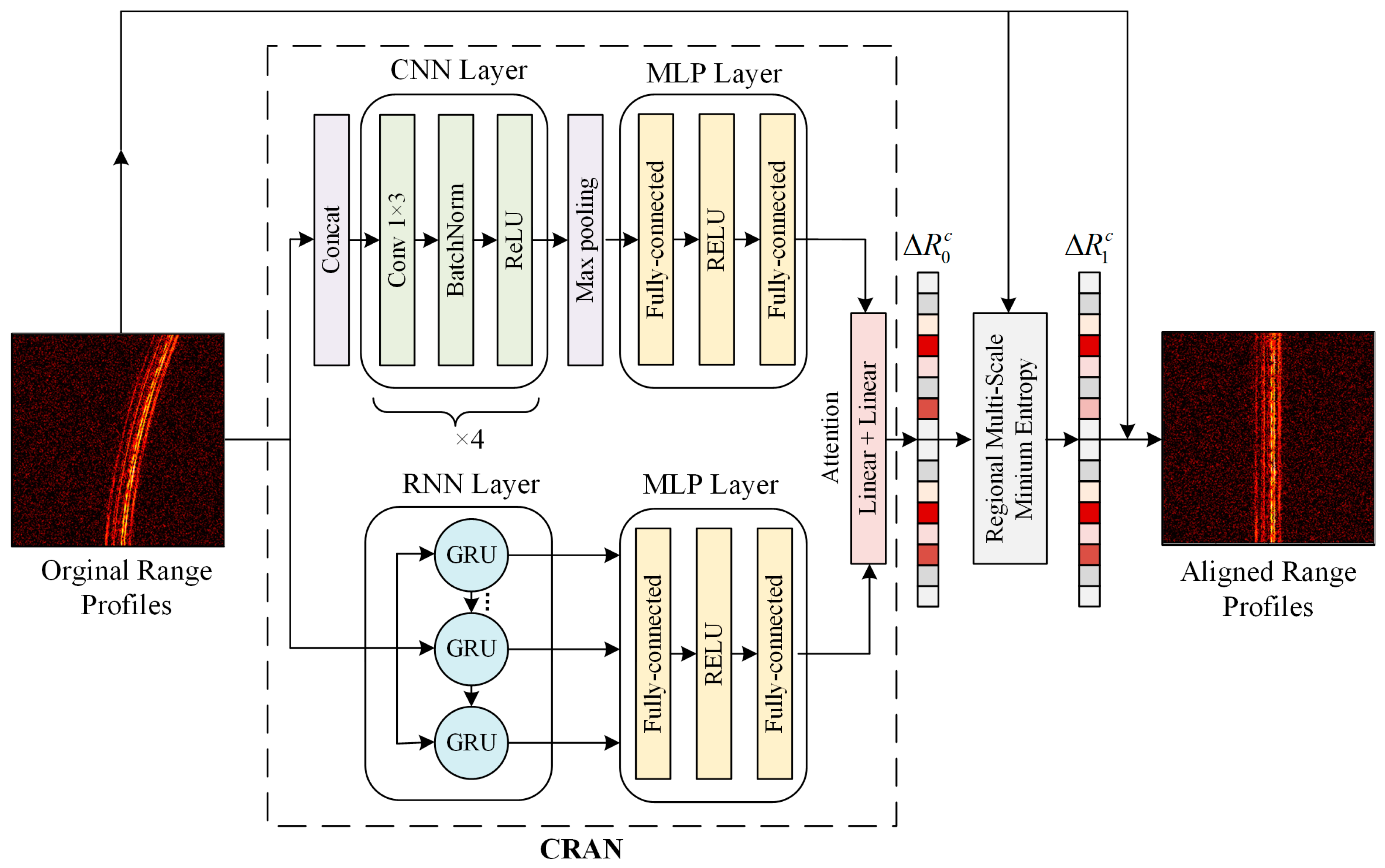
The proposed method combines a deep learning network with an enhanced minimum entropy approach. The deep learning network constructed in this paper is a CNN-RNN attention mechanism network (CRAN) architecture inspired by [23]. The network exploits CNN’s convolutional capability to focus on the texture details in the range profiles while using RNN’s memory gate capability to capture the temporal features of the range profiles at different slow time intervals. It employs an attention mechanism to integrate both results effectively, rapidly obtaining the coarse offset Δ R 0 c . Subsequently, through a regional multi-scale minimum entropy (RMSME) method for optimal solution searching, the fine offset Δ R 1 c is obtained. The overall structure of the proposed method is illustrated in Figure 2.

3.1. CRAN Architecture

The CRAN architecture is depicted in the wireframe in Figure 2. The input to the CRAN architecture is the normalized amplitude of the range profile, which is obtained by performing pulse compression on complex-valued raw echo data followed by magnitude extraction. The input image consists of n rows of slow-time range profiles and m columns of range cells, forming a two-dimensional data matrix of dimensions n × m. On the one hand, before entering the CNN layer, the first row of the data is duplicated n times and concatenated along the columns with the original data, forming a data matrix of dimensions n × 2m. The concatenated data are then input into the CNN layer. The purpose of this operation is to ensure that each row of data for different slow-time instances contains information from the starting moment, enhancing the learning of relevant correlation features. The CNN layer comprises four sub-modules, each consisting of a 1 × 3 convolutional layer, a Batch Normalization (BN) layer, and a Rectified Linear Unit (ReLU) layer. Through each module, the number of channels changes sequentially from 1 to 64, 128, 256, and 256. After exiting the CNN layer, the data undergo Max Pooling to reduce the 256 channels to 1 channel, resulting in feature data with dimensions [B, n, 2m], where B represents the batch size. The feature data are passed through a Multi-Layer Perceptron (MLP) layer for feature analysis. The MLP layer consists of a linear layer with dimensions [2m, m], an ReLU layer, and a linear layer with dimensions [m, 1], reducing the 2m-dimensional feature data to one dimension, resulting in an output with dimensions [B, n]. On the other hand, the raw data directly pass through an RNN layer, which comprises a GRU structure [22] with two hidden layers. The output yields feature data with dimensions [B, n, m]. The feature data are also subjected to feature analysis through an MLP layer. The MLP layer consists of a linear layer with dimensions [m, m], an ReLU layer, and a linear layer with dimensions [m, 1], resulting in an output with dimensions [B, n]. The outputs obtained from the CNN-MLP and RNN-MLP aspects are combined through an attention mechanism structure. The attention mechanism consists of two linear layers that weight the two outputs, with each linear layer having dimensions of [n, n]. Ultimately, the coarse offset Δ R 0 c is obtained.
The loss function L employed during the training of CRAN consists of two components: the mean squared error (MSE) and the maximum error (MaxE). The definitions for both are provided as shown in Equations (7) and (8). The use of MaxE is meaningful in that it guides the network to pursue lower mean errors while simultaneously aiming to minimize the maximum error. This approach is intended to reduce the search range in the subsequent RMSME method, thereby enhancing speed. The loss function L is represented by Equation (9).
MSE = 1 N R R L a b e l 2 2
MaxE = R R L a b e l
L = MSE + λ MaxE = 1 N R R L a b e l 2 2 + λ R R L a b e l
where 2 represents the L2 norm, represents the infinity norm, N represents the total number of samples, R L a b e l represents the label value for the translation offset, R represents the training result for the translation offset, and the coefficient is λ = 1 .

3.2. Regional Multi-Scale Minimum Entropy Method

The mechanism of the minimum entropy method is to find the target value that minimizes the entropy, where the target value corresponds to the offset caused by motion. The formula for calculating entropy is shown in Equation (10).
H ( S n , S n + 1 ) = m = 1 M p ( k , m ) log { p ( k , m ) }
where S n represents the nth range profile, M represents the number of range cells in a single range profile and p ( k , m ) is the probability distribution function, where m is the index of the range cell, and k is the offset value of the corresponding range cells between two range profiles. The definition of p ( k , m ) is given in Equation (11).
p ( k , m ) = S n ( m ) + S n + 1 ( m k ) m = 0 M 1 ( S n ( m ) + S n + 1 ( m k ) )
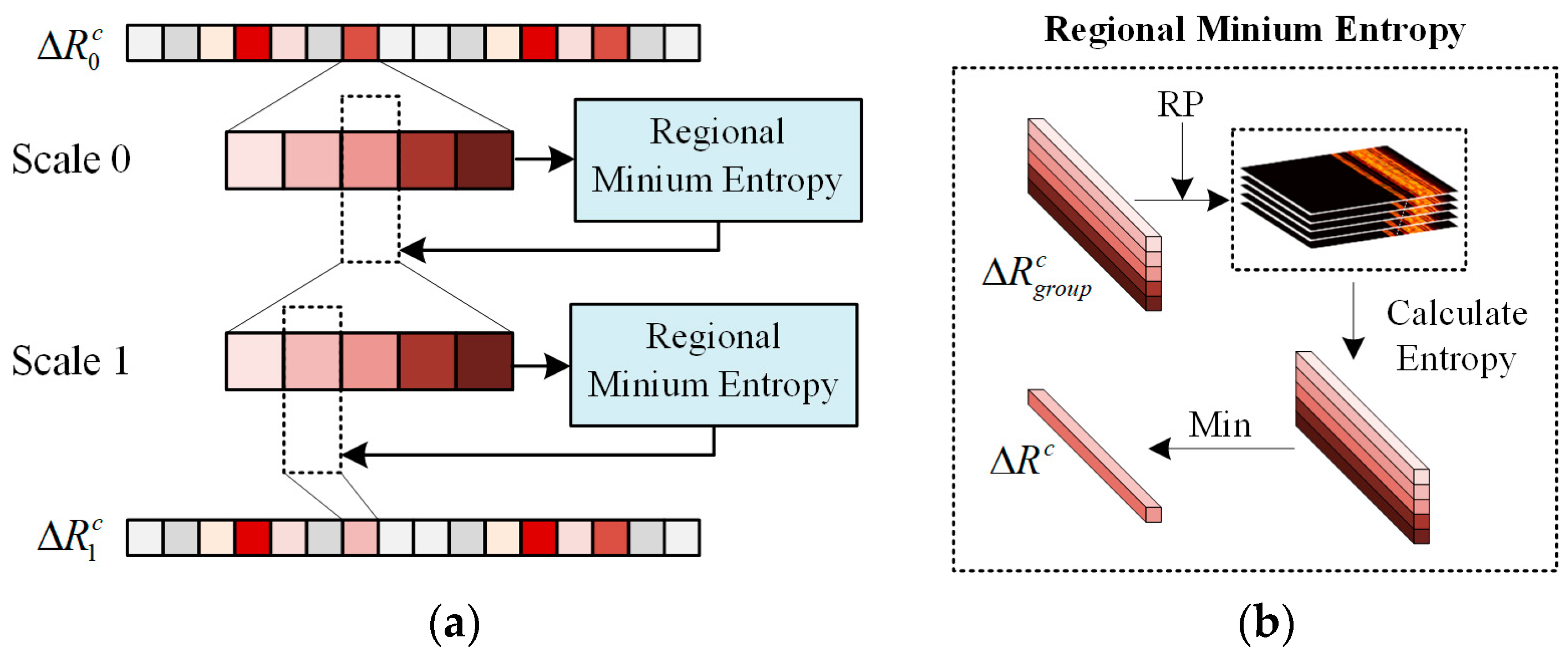
The regional multi-scale minimum entropy (RMSME) method is used to refine the localization further within the local range of the coarse offset Δ R 0 c , ultimately obtaining the fine offset Δ R 1 c . Multi-scale refers to the layered computation of minimum entropy (ME) at both the whole and sub-range resolution scales. The schematic diagram of the RMSME method is illustrated in Figure 3a. Scale 0 involves searching for the offset value that minimizes entropy at the full pixel scale. Scale 1 consists of searching for the offset value that minimizes entropy at the sub-pixel scale. Each instance of solving the regional minimum entropy (RME) involves a parallel computation for all range profiles, as depicted in Figure 3b. In RME, all the offset values that the range profiles need to traverse collectively form Δ R g r o u p c . The entropies are calculated after compensating the RP using Δ R g r o u p c , and the regional minimum is taken for each profile to obtain the offset for Δ R Min c . By iterating this several times at multiple scales, the fine offset Δ R 1 c can be obtained. This paper chooses two iterations. The parameters chosen for the RMSME method in this paper are presented in Table 1. The selection of ±15 range cells for Scale 0 was determined based on an analysis of metrics following the pre-training of the deep learning network. This range ensures the completeness of regional searches while reducing the search range.
The idea of employing RMSME emerged from observations in experiments solely utilizing deep learning networks. The generalization performance was imperfect, exhibiting favorable outcomes on the training set but manifesting irregular small offsets for untrained data. Utilizing RMSME addresses the optimization shortcomings in local areas. Simultaneously, compared to the traditional ME method’s global traversal, RMSME focuses only on a limited amount of local data. This enables the parallel computation of multiple range profiles. In this scenario, parallel computation requires only a modest amount of storage resources, facilitating the rapid attainment of local optimal solutions. Moreover, the multi-scale strategy enhances the precision of the range alignment process, accurately resolving translational errors at sub-range resolution scales rather than the common full-range resolution scale.

4. Experimental Section

4.1. Dataset and Experimental Setup

4.1.1. Dataset

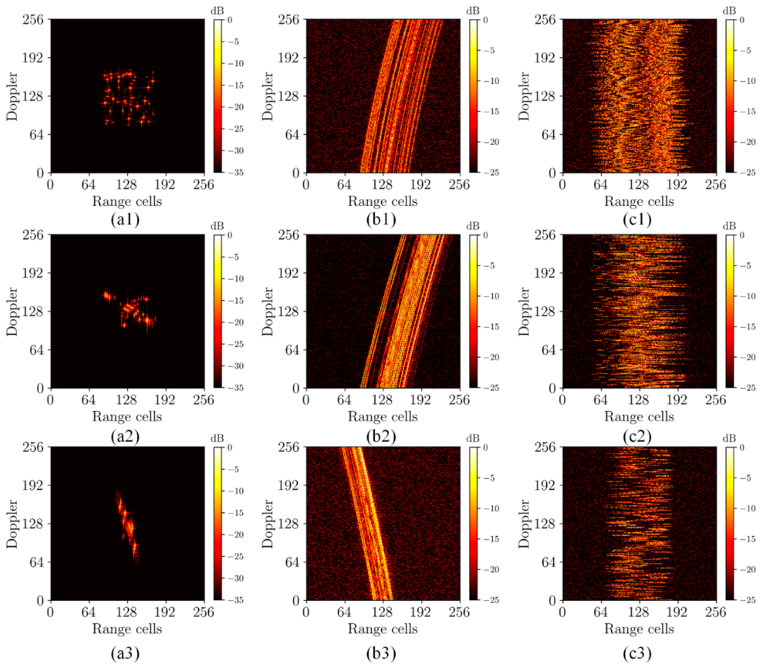
The experiments utilized three types of data to construct the dataset, including simulated echo data obtained from randomly distributed scatter points, a B727 model, and a satellite model. The purpose of configuring the dataset in this manner was to enhance the generalizability of the trained network. The inclusion of randomly distributed scattering points aims to prevent data from being confined to any specific intensity distribution. Incorporating the B727 scattering model is intended to ensure the efficacy of the training results for a meaningful feature distribution. Moreover, introducing satellite models further enhances the effectiveness of handling a large volume of scattering point data to match the measured data. The training set of the dataset comprises 2000 simulated data points from randomly distributed scatter points, 1000 from the B727 model, and 180 from the satellite model. The validation set of the dataset includes 1000 simulated data points from randomly distributed scatter points, 500 from the B727 model, and 90 from the satellite model. The dimensions of the data are 256 × 256. The simulated data encompass two modes: the trajectory motion and random motion. The initial echo data without range migration are generated according to the standard rotating platform model in which the noise is added with random signal-to-noise ratios ranging from 0 to 10 dB and downsampling with random sparsity rate ranging from 0 to 70 percent. The unaligned data are acquired by introducing motion-generated offsets onto the initial data phase. The assigned offsets are saved as labels. The schematic diagram depicting the composition of the dataset is illustrated in Figure 4. Figure 4(a1–a3), respectively, illustrate the focused imaging results of randomly distributed scatter points, the B727 model, and the satellite model. Figure 4(b1–b3) depict the range profile data of various models under trajectory motion conditions, while Figure 4(c1–c3) show the range profile data under random motion conditions.

4.1.2. Experimental Setup

The optimizer employed during the training process of the network is “Adam”, with an initial learning rate parameter set to 0.001. The scheduler used is “ReduceLROnPlateau”, with a factor parameter of 0.25, a patience parameter of 10, and the mode is set to “min”. The batch size of the training is 4. The criterion for stopping training is when the scheduler’s learning rate falls below 10−8. We mainly compared our method to the RNN-RA, CRAN-RA, and traditional ME range alignment (ME-RA) method, wherein the architectural components of RNN-RA and CRAN-RA employed for comparison were derived from the substructures proposed in this study. All the learning-based methods were trained on the same training set. For the quantitative evaluation of the output results, metrics such as entropy and contrast were employed for performance assessment. The definition of entropy (ENT) is provided in Equation (12).
ENT = m = 1 M n = 1 N S m n 2 m = 1 M n = 1 N S m n 2 ln ( S m n 2 m = 1 M n = 1 N S m n 2 )
Here, in the calculation of range profiles entropy (RE) for range profiles data, S m n represents the aligned range profiles result; in the calculation of ISAR image entropy (IE) for ISAR data, S m n represents the ISAR image result. A smaller value for both RE and IE indicates a better result.
The definition of contrast (CST) is provided by Equations (13)–(15).
CST = ω μ
where
ω = 1 M N m = 1 M n = 1 N S m n μ 2
and
μ = 1 M N m = 1 M n = 1 N S m n
where, in the calculation of range profiles contrast (RC), for range profiles data, S m n represents the aligned range profiles result; in the calculation of ISAR image contrast (IC) for ISAR data, S m n represents the ISAR image result. A larger value for both RC and IC indicates a better result.

4.2. Experimental Results and Analysis

4.2.1. Performance of Deep Learning Models

We first analyzed the performance of the convergence loss functions for several deep learning networks, including CNN, RNN, and CRAN. The compared CNN structure consists of the CNN layer and MLP layer in the upper part before the attention mechanism in Section 3.1. The CNN layer is a classic convolutional architecture similar to VGGnet. The compared RNN structure consists of the RNN layer and MLP layer in the lower part before the attention mechanism in Section 3.1. The RNN layer is the variant of GRU. This choice was made to conduct an ablation study with controlled variables. The reason why the number of epochs is different for training is that they have different speeds to reach the set termination target. The visualization of the training process is depicted in Figure 5. It can be observed from Figure 5a that the loss function of the CNN consistently remains higher than the others. Initially, the loss function of the RNN decreases rapidly, while as the network gradually converges, the loss function of the CRAN eventually becomes smaller. From Figure 5b,c, it can be observed that CRAN maintains excellent performance in both MSE and MaxE on the validation set. While CNN and RNN networks may exhibit instances where their performance falls below CRAN, CRAN is notably more stable and demonstrates better adaptability to unfamiliar data. On the training set, the advantage of CRAN over RNN is not pronounced, leading us to speculate that the RNN structure plays a significant role within CRAN. However, the results on the validation set highlight the generalization superiority and stability of CRAN, which are the primary reasons for our selection of CRAN. In addition to CNN and RNN, we also conducted ablation experiments on the concatenation structure before CNN in CRAN, with the results of the MSE and MaxR metrics presented in Table 2. The results indicate that the designed CRAN architecture, while ensuring optimal MSE, effectively confines the maximum error within 15 range cells. This means that the RMSME method only needs to search within a local range of ±15 cells in Scale 0.

4.2.2. Comparative Experiment and Analysis of Different RA Methods

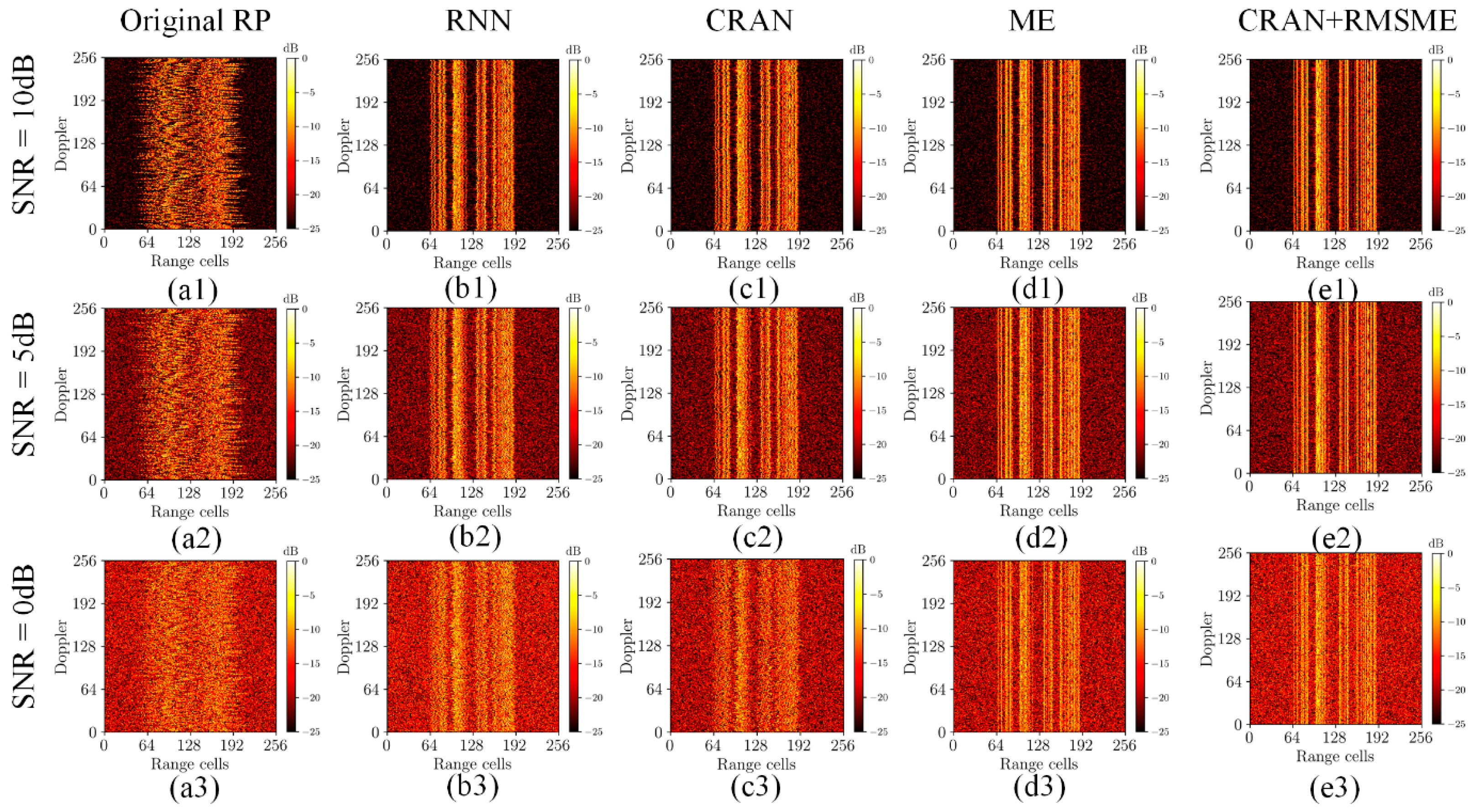
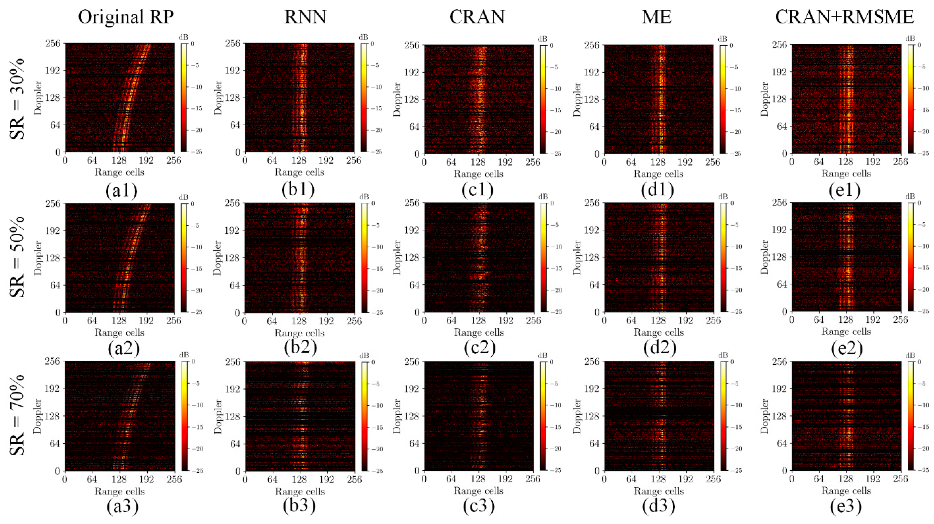
Then, the proposed method was compared with RNN-RA, CRAN-RA, and traditional ME-RA methods on the validation set, and the quantitative results of the evaluation metrics are presented in Table 3 and Table 4. Table 3 illustrates the comparison of results at different signal-to-noise ratios (SNRs) when the sparsity rate (SR) is set to 0. Table 4 presents the comparison of results at an SNR of 0 under different SRs. As the primary focus of this paper is not addressing SA-ISAR imaging issues, ISAR imaging was conducted solely on range profile data with a sparsity rate of 0. The comparisons of ISAR imaging results include IE and IC metrics. For sparse data, only RE and RC metrics were compared. The alignment results of different methods are illustrated in Figure 6 and Figure 7 to observe the effects of range alignment visually. Figure 6 presents the comparison of range alignment results for random motion data under different SNRs. Figure 7 presents the comparison of range alignment results for trajectory motion data under different SRs.
The performance evaluation results from Table 3 and Table 4 show that the proposed method in this paper consistently exhibited the minimum values for RE and IE and the maximum values for RC and IC under various SNRs. Similarly, this method achieved the minimum RE and maximum RC under different SRs. The results indicate that the proposed method in this study yields optimal outcomes. As evidenced by Figure 6 and Figure 7, the alignment results of the proposed method under different motion patterns are visually excellent. In Figure 7, as the SR increases, the noticeable deterioration in performance when utilizing the network independently may be attributed to the disruption of feature continuity caused by downsampling.
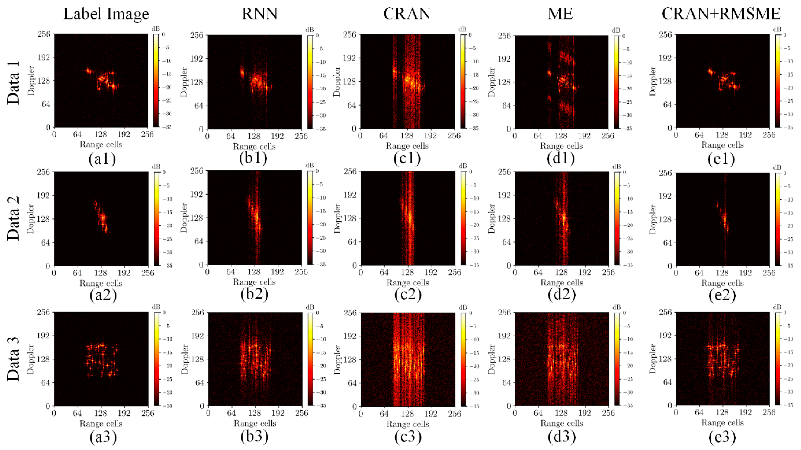
To further emphasize the advantages of the range alignment results in this study, ISAR imaging experiments were conducted. Following the alignment of range profile data, the phase gradient estimation [1] between profiles was conducted once, and azimuth compression was used to obtain the ISAR images. The ISAR imaging results of different methods are depicted in Figure 8. The figures show that the proposed method exhibits excellent focused imaging results, highlighting the effectiveness of the range alignment approach proposed in this study.
In Figure 8, the imaging quality of both RNN and CRAN appears to be inferior to the references [24,25], which could possibly be attributed to discrepancies in the training dataset and network architecture parameters. Given that this study does not prioritize the pursuit of optimal network performance, this part of deep learning networks did not delve deeply into exploring the impact of network parameters. The above results indicate that traditional methods still possess competitiveness in terms of robustness and accuracy. However, while surpassing traditional methods in robustness and accuracy, the approach proposed in this paper exhibits significant advantages in processing speed. The runtime comparison was conducted among the proposed methods, the traditional ME method, the GPU-accelerated ME (GME) method, RNN-RA method, and the CRAN-RA method. The experiments were executed on a 3.0GHz Intel i7-9700 CPU (manufacture: Intel, Santa Clara, CA, USA) and a Nvidia GeForce RTX 2080 SUPER GPU (manufacture: Nvidia, Santa Clara, CA, USA). The results are presented in Table 5. It is evident from the results that the use of the deep learning network and RMSME method significantly improved the processing speed compared with the traditional ME method and the GPU-accelerated ME (GME) method. At the same time, there was no unacceptable degradation compared to RNN-RA and CRAN-RA.
In summary, compared to methods solely relying on deep learning networks, the combination of the deep learning network and RMSME method addresses the issue of reduced prediction accuracy when there is a significant disparity between input data and training data. Simultaneously, compared to using only the ME method, the combination of the deep learning network and RMSME method eliminates the need for a search across the entire range. Instead, it refines the localization based on the network’s coarse estimation and performs a multi-scale ME search locally to achieve precise alignment at sub-range resolution. This significantly reduces the time consumption during the search process.

4.3. Verification of Measured Data

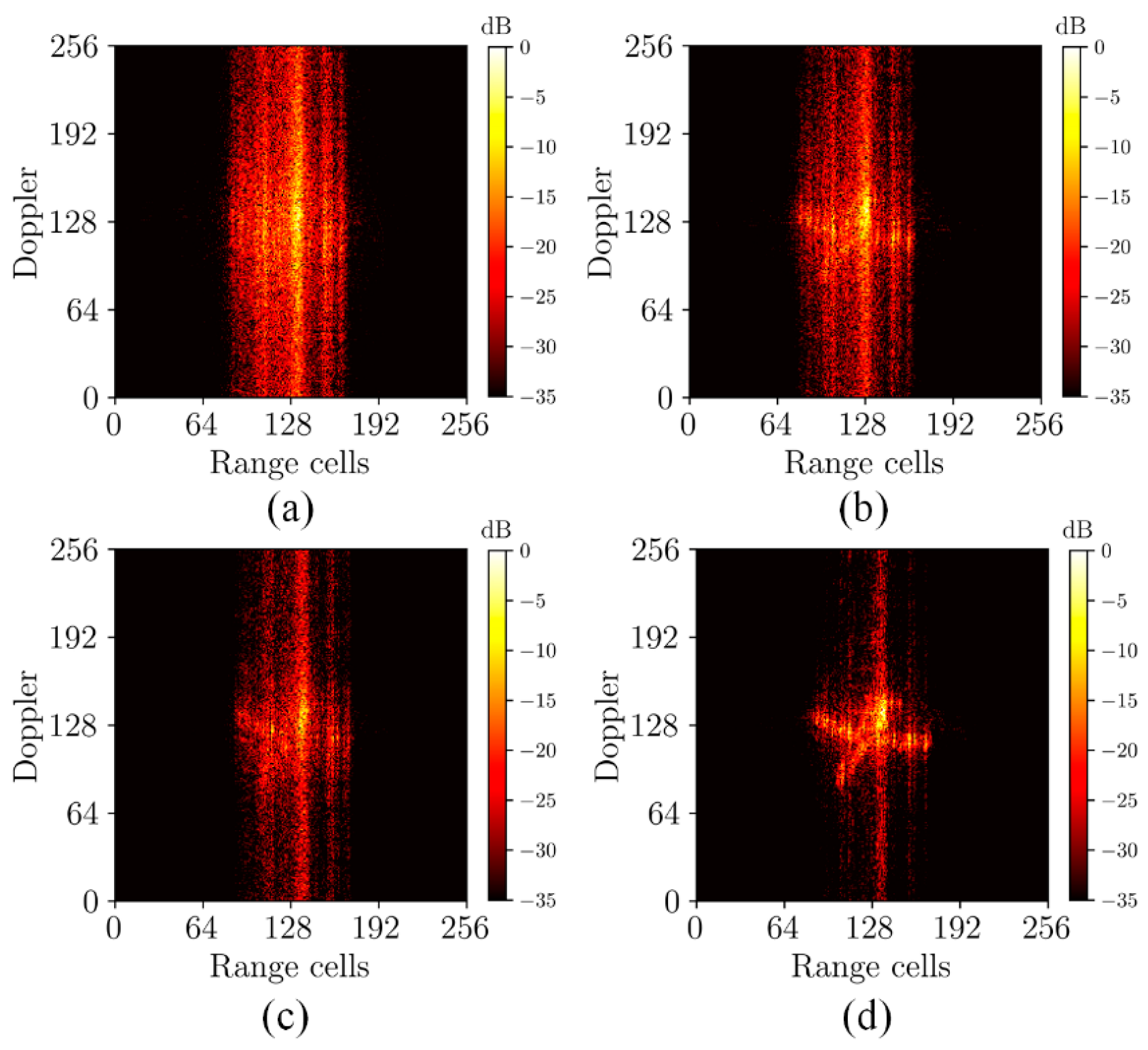
To demonstrate the proposed range alignment method’s practical value, we validated using measured data. Figure 9 illustrates the range alignment results of Yak-42 real measured data under different methods. Figure 10 displays the ISAR imaging results after range alignment, using the same imaging approach as depicted in Figure 8. Table 6 presents the quantitative results of measured data under different methods.
The quantitative evaluation results show that the proposed method has minimum RE, IE, and maximum IC. Based on the results from the measured data, although a tailing effect persisted due to the simplicity of the phase correction method, the images exhibit superior focusing effects, presenting clearer targets and higher image quality compared to other methods. This indicates the superior alignment effect of the proposed approach. The validation experiment with measured data confirms the reliability of the proposed method in practical applications.

5. Conclusions

This paper proposes a fast and robust range alignment method based on CRAN and the regional multi-scale minimum entropy method. This approach utilizes CRAN for rapid coarse alignment and employs the RMSME method for fine alignment. The proposed method effectively addresses the current challenges of poor generalization in deep learning networks and the low efficiency of traditional minimum entropy methods. Simulation experiments demonstrate that the proposed method exhibits minimum entropy and maximum contrast, indicating a significant improvement in range alignment performance. Experimental results with measured data validate the practical utility of the proposed method. This work still has some limitations. The construction of the training and validating sets could be further improved by incorporating more measured and simulated data to enhance the practical value. Additionally, the Scale 0 parameter in the RMSME structure was constrained by the performance of the deep learning network. When encountering certain data that degrade network performance, the Scale 0 parameter increased, resulting in a decrease in the speed of the proposed method. Future improvements to the network structure could enhance the running speed to meet the demands of some real-time computation applications. While there will be future advancements in deep learning networks that could outperform CRAN, the combined strategy designed in this paper with RMSME integration holds broad applicability. This research provides reference significance for the possibility of the joint application of deep learning methods and traditional methods in the RA process.

Author Contributions

Conceptualization, H.W.; Formal analysis, Q.N.; Funding acquisition, H.W.; Investigation, Q.N., Z.Y. and Z.W.; Methodology, Q.N.; Project administration, H.W.; Software, Q.N.; Supervision, H.W.; Validation, Q.N., Z.Y. and Y.L.; Visualization, Q.N., Z.Y. and Z.W.; Writing—original draft, Q.N.; Writing—review and editing, Q.N. All authors have read and agreed to the published version of the manuscript.

Funding

This research was funded by National Natural Science Foundation of China, grant number 61705220.

Data Availability Statement

Data are contained within the article.

Conflicts of Interest

The authors declare no conflicts of interest.

References

  1. Ozdemir, C. Inverse Synthetic Aperture Radar Imaging with Matlab Algorithms; Wiley: Hoboken, NJ, USA, 2012; pp. 300–316. [Google Scholar]
  2. Chen, V.C. Inverse Synthetic Aperture Radar Imaging: Principles, Algorithms and Applications; Institution of Engineering and Technology: Stevenage, UK, 2014; Volume 55, p. 56. [Google Scholar]
  3. Zhu, D.; Wang, L.; Yu, Y.; Tao, Q.; Zhu, Z. Robust ISAR range alignment via minimizing the entropy of the average range profile. IEEE Geosci. Remote Sens. Lett. 2009, 6, 204–208. [Google Scholar]
  4. Zhang, L.; Sheng, J.l.; Duan, J.; Xing, M.D.; Qiao, Z.J.; Bao, Z. Translational motion compensation for ISAR imaging under low SNR by minimum entropy. EURASIP J. Adv. Signal Process. 2013, 2013, 33. [Google Scholar] [CrossRef]
  5. Zhang, S.; Liu, Y.; Li, X. Fast entropy minimization based autofocusing technique for ISAR imaging. IEEE Trans. Signal Process. 2015, 63, 3425–3434. [Google Scholar] [CrossRef]
  6. Wang, R.; Zeng, T.; Hu, C.; Yang, J. Accurate range profile alignment method based on minimum entropy for inverse synthetic aperture radar image formation. Iet Radar Sonar Navig. 2016, 10, 663–671. [Google Scholar] [CrossRef]
  7. Ligori, D.; Wagner, S.; Fabbrini, L.; Greco, M.; Bieker, T.; Pinelli, G.; Brüggenwirth, S. Nonparametric ISAR autofocusing via entropy-based Doppler centroid search. IEEE Geosci. Remote Sens. Lett. 2018, 15, 1725–1729. [Google Scholar] [CrossRef]
  8. Wang, J.; Zhang, L.; Du, L.; Yang, D.; Chen, B. Noise-Robust Motion Compensation for Aerial Maneuvering Target ISAR Imaging by Parametric Minimum Entropy Optimization. IEEE Trans. Geosci. Remote Sens. 2019, 57, 4202–4217. [Google Scholar] [CrossRef]
  9. Du, Y.; Jiang, Y. Parametric translational motion compensation of spaceborne ISAR imagery for earth-orbit targets based on parabola detection and entropy minimization. Remote Sens. Lett. 2021, 12, 160–168. [Google Scholar] [CrossRef]
  10. Wang, J.; Li, Y.; Song, M.; Huang, P.; Xing, M. Noise Robust High-Speed Motion Compensation for ISAR Imaging Based on Parametric Minimum Entropy Optimization. Remote Sens. 2022, 14, 2178. [Google Scholar] [CrossRef]
  11. Ding, Z.; Zhang, G.; Zhang, T.; Gao, Y.; Zhu, K.; Li, L.; Wei, Y. An improved parametric translational motion compensation algorithm for targets with complex motion under low signal-to-noise ratios. IEEE Trans. Geosci. Remote Sens. 2022, 60, 5237514. [Google Scholar] [CrossRef]
  12. Liu, F.; Huang, D.; Guo, X.; Feng, C. Noise-Robust ISAR Translational Motion Compensation via HLPT-GSCFT. Remote Sens. 2022, 14, 6201. [Google Scholar] [CrossRef]
  13. Hu, C.Y.; Wang, L.; Li, Z.; Zhu, D.Y. Inverse Synthetic Aperture Radar Imaging Using a Fully Convolutional Neural Network. IEEE Geosci. Remote Sens. Lett. 2020, 17, 1203–1207. [Google Scholar] [CrossRef]
  14. Wei, S.; Liang, J.; Wang, M.; Zeng, X.; Shi, J.; Zhang, X. CIST: An Improved ISAR Imaging Method Using Convolution Neural Network. Remote Sens. 2020, 12, 2641. [Google Scholar] [CrossRef]
  15. Shi, H.; Liu, Y.; Guo, J.; Liu, M. ISAR autofocus imaging algorithm for maneuvering targets based on deep learning and keystone transform. J. Syst. Eng. Electron. 2020, 31, 1178–1185. [Google Scholar]
  16. Wang, L.; Wang, L.; Zhu, D. An ISAR Autofocus Imaging Algorithm Based on FCN and Transfer Learning. In Proceedings of the 2023 24th International Radar Symposium (IRS), Berlin, Germany, 24–26 May 2023. [Google Scholar]
  17. Wang, Y.; Feng, C.; Zhang, Y.; He, S. Translational motion compensation of space micromotion targets using regression network. IEEE Access 2019, 7, 155038–155047. [Google Scholar] [CrossRef]
  18. Liu, Z.; Yang, S.; Gao, Q.; Feng, Z.; Wang, M.; Jiao, L. AFnet and PAFnet: Fast and Accurate SAR Autofocus Based on Deep Learning. IEEE Trans. Geosci. Remote Sens. 2022, 60, 5238113. [Google Scholar] [CrossRef]
  19. Li, X.; Bai, X.; Zhou, F. High-Resolution ISAR Imaging and Autofocusing via 2D-ADMM-Net. Remote Sens. 2021, 13, 2326. [Google Scholar] [CrossRef]
  20. Li, M.; Wu, J.; Huo, W.; Li, Z.; Yang, J.; Li, H. STLS-LADMM-Net: A deep network for SAR autofocus imaging. IEEE Trans. Geosci. Remote Sens. 2022, 60, 5226914. [Google Scholar] [CrossRef]
  21. Li, R.Z.; Zhang, S.H.; Zhang, C.; Liu, Y.X.; Li, X. Deep Learning Approach for Sparse Aperture ISAR Imaging and Autofocusing Based on Complex-Valued ADMM-Net. IEEE Sens. J. 2021, 21, 3437–3451. [Google Scholar] [CrossRef]
  22. Pu, W. SAE-Net: A Deep Neural Network for SAR Autofocus. IEEE Trans. Geosci. Remote Sens. 2022, 60, 5220714. [Google Scholar] [CrossRef]
  23. Wei, S.J.; Liang, J.D.; Wang, M.; Shi, J.; Zhang, X.L.; Ran, J.H. AF-AMPNet: A Deep Learning Approach for Sparse Aperture ISAR Imaging and Autofocusing. IEEE Trans. Geosci. Remote Sens. 2022, 60, 5206514. [Google Scholar] [CrossRef]
  24. Yuan, Y.; Luo, Y.; Kang, L.; Ni, J.; Zhang, Q. Range alignment in ISAR imaging based on deep recurrent neural network. IEEE Geosci. Remote Sens. Lett. 2022, 19, 4022405. [Google Scholar] [CrossRef]
  25. Li, W.; He, Q.; Li, K.; Yuan, Y.; Luo, Y. ISAR range alignment under sparse aperture condition based on CRAN. In Proceedings of the 2022 IEEE 5th International Conference on Electronic Information and Communication Technology (ICEICT), Hefei, China, 21–23 August 2022. [Google Scholar]
Figure 1. The schematic diagram of relative motion (Position 1 represents the starting point of the motion, Position 2 represents the endpoint of the equivalent rotation, and Position 3 represents the actual endpoint).
Remotesensing 16 03677 g001
Figure 2. The overall structure of the proposed method.
Remotesensing 16 03677 g002
Figure 3. The RMSME method. (a) The schematic diagram of the RMSME method; (b) regional minimum entropy structure.
Remotesensing 16 03677 g003
Figure 4. The schematic diagram of the dataset. (a1a3) The focused imaging results of randomly distributed scatter points, the B727 model, and the satellite model; (b1b3) the range profile data of various models under trajectory motion conditions; and (c1c3) the range profile data of various models under random motion conditions.
Remotesensing 16 03677 g004
Figure 5. Visualization of the training process: (a) variation in the loss function on the training set; (b) variation in the MSE on the validation set; and (c) variation in the MaxE on the validation set.
Remotesensing 16 03677 g005
Figure 6. The comparison of range alignment results for random motion data under different SNRs. (a1a3) Original range profiles under random motion. (b1b3) The range alignment results of RNN-RA. (c1c3) The range alignment results of CRAN-RA. (d1d3) The range alignment results of ME-RA. (e1e3) The range alignment results of the proposed method.
Remotesensing 16 03677 g006
Figure 7. The comparison of range alignment results for trajectory motion data under different SRs. (a1a3) Original range profiles under trajectory motion; (b1b3) the range alignment results of RNN-RA; (c1c3) the range alignment results of CRAN-RA; (d1d3) the range alignment results of ME-RA; and (e1e3) the range alignment results of the proposed method.
Remotesensing 16 03677 g007
Figure 8. The ISAR imaging results of different methods under different data. (a1a3) ISAR imaging results using the label. (b1b3) The ISAR imaging results after RNN-RA. (c1c3) The ISAR imaging results after CRAN-RA. (d1d3) The ISAR imaging results after ME-RA. (e1e3) The ISAR imaging results after the proposed RA method.
Remotesensing 16 03677 g008
Figure 9. The range alignment results of Yak-42 real measured data under different methods. (a) Original range profiles. (b) The range alignment results of RNN-RA. (c) The range alignment results of CRAN-RA. (d) The range alignment results of ME-RA. (e) The range alignment results of the proposed method.
Remotesensing 16 03677 g009
Figure 10. The ISAR imaging results of measured data. (a) The ISAR imaging results after RNN-RA. (b) The ISAR imaging results of CRAN-RA. (c) The ISAR imaging results after ME-RA. (d) The ISAR imaging results after the proposed RA method.
Remotesensing 16 03677 g010
Table 1. The parameters of the RMSME method.
NameStart (Range Cells)Step (Range Cells)Stop (Range Cells)
Scale 0−15115
Scale 1−10.11
Table 2. Comparison of the convergence performance of loss functions for different networks.
MethodMSEMaxE
CNN1.12928.74
RNN1.08222.21
CRAN without Concatenation0.99315.88
CRAN0.77813.24
Table 3. The quantitative results at different SNRs when SR is 0.
SNR (dB)MethodRERCIEIC
RNN9.30991.32538.18341.6854
10CRAN9.31091.32508.81431.4544
ME9.31081.32497.87171.7218
CRAN+RMSME9.30181.32916.91362.1157
RNN9.70901.01779.02841.1758
5CRAN9.70911.01769.65001.0163
ME9.70881.01788.62251.2565
CRAN+RMSME9.70171.02047.88121.4440
RNN10.21300.744710.10340.7643
0CRAN10.21290.744810.32770.6976
ME10.21320.74479.78680.8378
CRAN+RMSME10.21030.74589.58800.8784
Table 4. The quantitative results at different SRs when SNR is 0.
SR (%)MethodRERC
RNN9.86080.7447
30CRAN9.86100.7447
ME9.86060.7448
CRAN+RMSME9.83940.7597
RNN9.51980.7447
50CRAN9.51970.7448
ME9.51950.7449
CRAN+RMSME9.49750.7597
RNN9.01110.7449
70CRAN9.01100.7450
ME9.01080.7451
CRAN+RMSME8.98940.7596
Table 5. The runtime comparison experiment.
MethodAverage Time per Frame (s)
ME11.928
GME0.152
RNN0.0105
CRAN0.0106
CRAN+RMSME0.0390
Table 6. The quantitative results of measured data under different methods.
MethodRERCIEIC
RNN8.93511.70938.48751.8812
CRAN8.93821.70678.63671.8064
ME8.93241.70948.50401.8461
CRAN+RMSME8.93161.70817.41922.4769
Disclaimer/Publisher’s Note: The statements, opinions and data contained in all publications are solely those of the individual author(s) and contributor(s) and not of MDPI and/or the editor(s). MDPI and/or the editor(s) disclaim responsibility for any injury to people or property resulting from any ideas, methods, instructions or products referred to in the content.