Exploration of the Urbanization Process and Its Impact on Vegetation in 125 Resource-Based Cities in China and Comparison with Other Cities

Abstract

Resource-based cities (RBCs) in China are at a historic juncture in their transformative development. Observing and assessing the role of the resource curse in urban expansion and greening is crucial for the sustainable development of these cities. This study proposes a new framework to extract urban boundary data from 2000 to 2020 in China. Utilizing these data, we analyzed differences in urban expansion intensity and urban vegetation cover between 125 RBCs and 223 non-RBCs. We found the following: (1) While urban areas in China experienced steady growth from 2000 to 2020, the urban area expansion rates of RBCs lagged behind those non-RBCs located in the same geographical areas except in South China, with the lowest annual expansion rate of 1.18% occurring in the Northeast. (2) Although the existing urban areas in some cities show a greening trend, both existing and new urban areas in China are predominantly characterized overall by browning. Surprisingly, RBCs exhibit a stronger greening trend than non-RBCs, particularly in Northwestern China. (3) There is a nuanced interplay and coexistence between resource dependency and urban expansion, with a specific negative correlation when resource dependency is very high or very low. This study provides a novel method and approach for urban boundary delineation. It offers new insights into the developmental characteristics of RBCs, enriching the theoretical framework of resource curse research and supporting the green development of RBCs with robust data.

1. Introduction

Urbanization has emerged as a prominent feature and inevitable trend in global development today, profoundly influencing the lives of most of the world’s citizens [1,2]. It fosters economic growth, improves human settlements, drives societal transformations, and presents unprecedented challenges to urban planning, environmental protection, and resource management [3,4]. Resource-based cities (RBCs), characterized by industries dominated by the extraction and processing of minerals and forests, have significantly contributed to socioeconomic development and national industrialization [5]. Their urbanization has flourished alongside the robust growth of resource industries. However, because of the non-renewable nature of resources and imbalances in industrial structures, abundant resources have paradoxically not promoted high-quality economic development in these cities but instead have hindered it, leading to the phenomenon known as the resource curse [6,7]. Overcoming this dilemma to achieve urban transformation and sustainable development represents these cities’ most significant challenge.

Since entering the 21st century, China has experienced rapid urbanization [8]. RBCs have provided a continuous energy supply vital for national economic development, yet the resource curse phenomenon has become increasingly evident. Numerous studies have explored the drivers, formation processes, and impacts of the resource curse on socioeconomic development, proposing initiatives and plans to counteract it [9,10]. At the national level, policies such as the National Sustainable Development Plan for Resource-based Cities (2013–2020) (referred to as the Plan) and the Fourteenth Five-Year Plan for High-Quality Development of Resource-Based Regions have been implemented to promote the transformation of RBCs [11,12]. However, the specific effects of the resource curse on urban expansion and green development remain unclear.

Currently, RBCs at the prefecture level or above constitute approximately one-third of all cities at or above the prefecture level in China. Because of differences in resource utilization and dependence, foundational development conditions, and directions for transformation, there are specific differences in urban area, expansion intensity, and their impacts on the ecological environment among various RBCs. Additionally, significant distinctions between resource-based and non-resource-based cities present a topic worthy of in-depth exploration. However, government management departments and academia primarily focus on qualitative discussions or quantitative analyses based on traditional socioeconomic statistical data [13,14]. These traditional data sources often lack spatial visualization and suffer from inconsistencies in statistical standards, making it challenging to reflect the development dynamics of RBCs fully and objectively across regions, categories, and levels. Long-term, high spatiotemporal consistency multi-source data provided by satellite Earth observation offers new perspectives and possibilities for uncovering the urbanization processes and ecological changes in RBCs [15,16].

In China, urban administrative jurisdictions typically encompass extensive rural and non-urban areas. Therefore, the study of urbanization in China should not merely consider administrative boundaries; rather, it necessitates a more precise delineation of urban entities to assess the relationship between vegetation and other indicators with urban expansion [17]. The current key issue lies in the automated and accurate identification of urban boundaries, which is crucial for a deeper understanding and assessment of the role of the resource curse in urban development and the mechanisms and effects of vegetation change in response.

Current research primarily focuses on accurately identifying boundaries for a single or a few cities [18,19,20] or roughly estimates urban extents by analyzing land use data and impervious surface data to study the relationship between urbanization and urban environmental changes [21,22,23]. Accurately, conveniently, and uniformly standardizing the identification of urban boundaries is crucial for advancing urbanization research and facilitating standardized comparisons both between and within countries regarding Sustainable Development Goal (SDG) 11—sustainable cities and communities. Many organizations and scholars have recognized the importance and urgency of this issue and have initiated related research. For example, the Joint Research Centre (JRC) of the European Commission has created the 1 km resolution Urban Centre Database (GHS-UCDB) [24]. Li [25] crafted Global Urban Boundary (GUB) using the Global Artificial Impervious Area (GAIA) data. Hafner [26] utilized Sentinel-1 and Sentinel-2 satellite data, applying a novel Semi-Supervised Learning approach to enhance global urban mapping. These achievements provide significant data resources for global or regional-scale urbanization research. However, extracting urban boundaries on a worldwide scale still presents considerable challenges. The definitions, formation processes, and morphologies of cities vary significantly across countries, making it particularly difficult to use a unified method to delineate urban boundaries. Current studies often define urban areas using building density and population concentration indicators. However, in China, particularly in the eastern regions, towns are densely distributed, and contiguous rural areas also exhibit characteristics of high building and population densities, making them difficult to distinguish from urban areas.

In this context, our study utilizes Global Human Settlement Layer (GHS-BUILT-S) building and population (GHS-POP) data, combined with specific definitions and developmental characteristics of Chinese cities, to develop a top-down automated method for urban boundary identification. We created datasets for 2000, 2005, 2010, 2015, and 2020 at 100 m resolution based on GHSL, named GCUB (GHSL-Based China’s Urban Boundaries). Based on these data, we explored the following questions:

(1) How do the rates of urban area expansion in RBCs compare to those in non-RBCs?

(2) What are the characteristics of urban greening in China’s RBCs compared to non-RBCs?

(3) What is the relationship between resource production and urban expansion?

This study aims to provide macro-level statistical data on the spatial development of RBCs for national policymaking. The objective is to inform top-level strategic planning that promotes RBCs’ green and sustainable development. Additionally, it offers specific urban spatial expansion maps to support local administrative bodies in formulating detailed plans.

2. Study Area and Datasets

2.1. Study Area

According to the Plan issued by the Chinese government in 2013, a total of 126 prefecture-level cities in China were designated as RBCs [13]. Among these, Laiwu (an RBC) was merged with Jinan (a non-RBC and the capital of Shandong Province) in 2019 because of administrative reorganization. Consequently, this study analyzes the remaining 125 prefecture-level RBCs. The distribution of these RBCs is shown in Figure 1.

2.2. Datasets

The Global Human Settlement Layer (GHSL) is a worldwide dataset of human settlement spatial information developed by the JRC of the European Commission [27]. Primarily utilizing Landsat and Sentinel-2 as baseline data sources, the GHSL produces GHS-BUILT-S, GHSL-POP, and Settlement Model layers (GHS-SMOD) for the years 1975 to 2030 in five-year increments. The GHSL has been validated for high accuracy [28] and is widely used in studies on urbanization [29], population research [30], and environmental change assessments [31]. For our study, we used the multi-temporal GHS-BUILT-S and GHSL-POP data with a resolution of 100 m for the years 2000, 2005, 2010, 2015, and 2020. We selected widely used urban boundary datasets (

Table 1. The characteristics of urban boundary datasets used in this study.

Dataset	GHS-SOMD [27]	GUE [33]	GUB [25]	GHUB [34]
Resolution	1 km	500 m	30 m	30 m
Years Covered	1975–2020	2000–2020	1990–2020	2018
Area Covered	Global	Global	Global	Global
Data Source	GHS-BUILT-S and GHS-POP	Nighttime light data	Impervious surface data	Impervious surface data

), including GHSL-SOMD, Global Urban Entities (GUE), GUB, GHUB, and our developed GCUB for comparison. GHUB and GHS-SMOD are hierarchical urban boundary data, and we used their Urban Centre layers for comparison. Additionally, we used MODIS MOD09GA [32] data to calculate vegetation coverage. The urban panel data used to measure resource dependency were sourced from the China Urban Statistical Yearbook.

3. Methodology

3.1. GCUB Generation Method

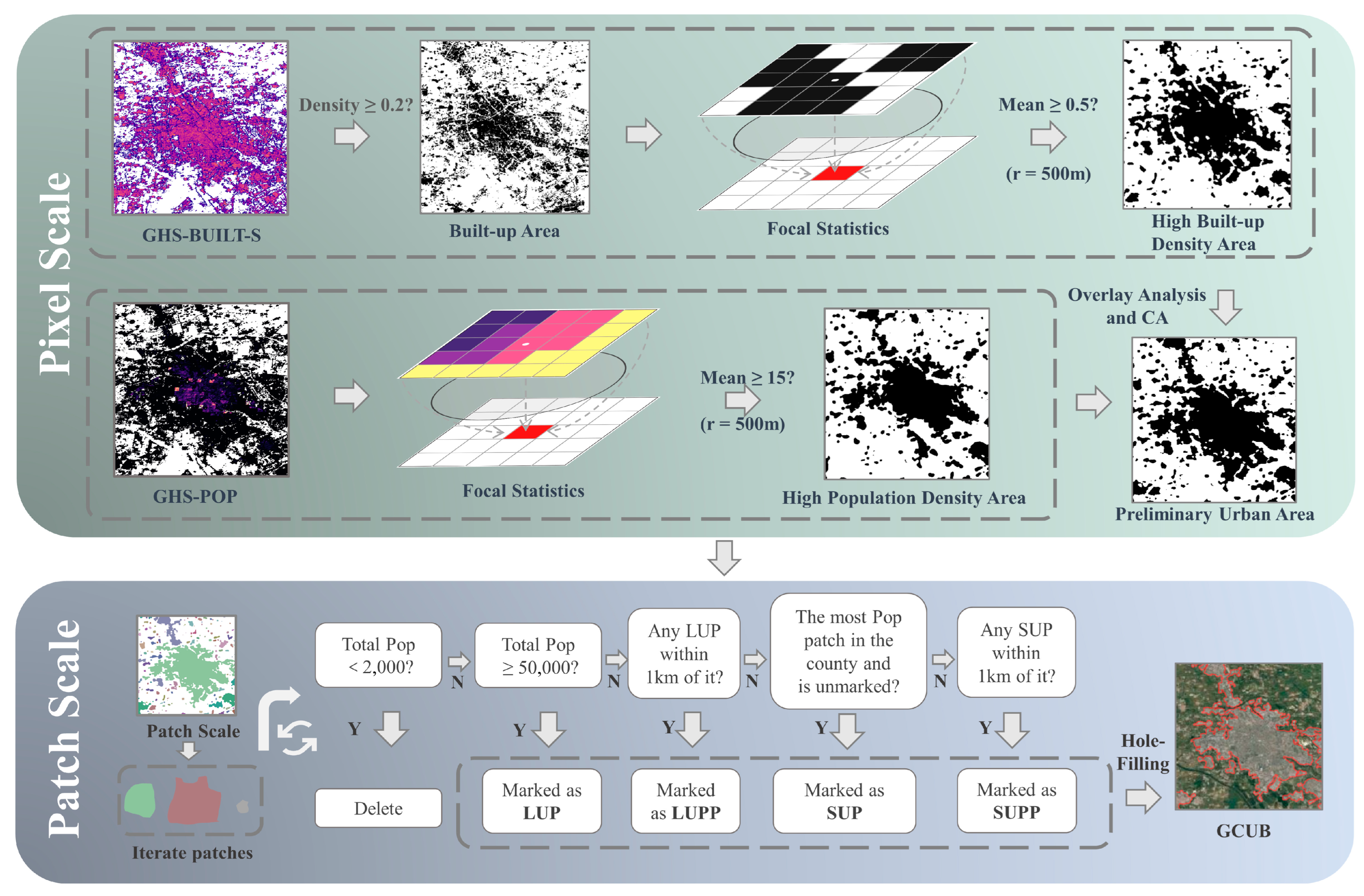
We utilized the GHS-BUILT-S and GHS-POP datasets, combined with specific definitions and developmental characteristics of Chinese cities, to propose and apply a method for urban boundary identification, which was used to map the urban boundary datasets for the years 2000, 2005, 2010, 2015, and 2020 in China. The method consists of the following two main parts: (1) On the Google Earth Engine (GEE) platform, the neighborhood mean method is applied to process GHS-BUILT-S and GHSL-POP data to identify areas with high building and population density, revealing potential urban patches. (2) Urban Hierarchical Screening Algorithm (UHSA): Using Arcpy, a Python library for geospatial analysis provided by ArcGIS Pro 3.0, these potential urban patches are processed, integrating city administrative boundary vector data and considering factors such as the total population of the patches and relative distances, employing a top-down filtering strategy to identify urban patches of different levels gradually, thus delineating urban boundaries. The flowchart is shown in Figure 2, and the detailed steps are as follows:

Step 1: Generating high-density built-up areas.

The DN value of each grid in the GHS-BUILT-S dataset represents the probability that the grid is a built-up area [35]. Following research by Uhl [36] and Corbane [37], a threshold of 0.2 is effectively used to identify built-up areas. This study used this threshold to process the GHS-BUILT-S data, generating a binary image $f_1$ (Equation (1)) to differentiate between built-up and non-built-up areas.

$$f_1=\left\{\begin{array}{c}0, f_b\left(x,y\right)<0.2\\ 1, f_b\left(x,y\right)\ge 0.2\end{array}\right.$$

(1)

where $f_b\left(x,y\right)$ represents the DN value of the GHS-BUILT-S data at location $(x,y)$.

The neighborhood mean method was applied for data smoothing and edge enhancement, using a window size of 11 × 11 pixels equivalent to a convolution kernel with an edge length of nearly 1 km [38]. This process generated each pixel’s built-up intensity (BI) (Equation (2)). A threshold of 0.5 [39] was then used to divide the map into areas of high and low built-up intensity, producing a binary image $f_2$ (Equation (3)).

$$BI\left(x,y\right)=f_{\mathrm{b}-\mathrm{avg}}\left(x,y\right)={\displaystyle \frac{1}{n^2}}{\sum }_{i=-k}^k{\sum }_{j=-k}^k{f}_1\left(x+i,y+j\right)$$

(2)

$$f_2=\left\{\begin{array}{c}0, BI\left(x,y\right)<0.5\\ 1, BI\left(x,y\right)\ge 0.5\end{array}\right.$$

(3)

where $f_1\left(x+i,y+j\right)$ is the DN value of the $f_1$ image at the position $(x+i,y+j)$ and $f_{\mathrm{b}-\mathrm{avg}}\left(x,y\right)$ is the DN value at position (x, y) after local averaging. Since $f_1$ is a binary image, this value also represents the built-up intensity of that pixel, namely, $BI(x,y)$. $n^2$ is the total number of pixels within the neighborhood and $k=(n-1)/2$ means the distance from the center pixel to the edge.

Step 2: Generating high-density population areas.

The GHS-POP dataset provides the total population within each grid. The same size convolution kernel was applied to these data for neighborhood mean analysis to achieve data smoothing and edge enhancement (Equation (4)). Zhou [40] suggested using a threshold of 1500 people/km² to delineate urban extents in China, which was also applied in a 2021 research report on urban–rural definitions by six major international organizations, including the European Union (EU) and the Food and Agriculture Organization of the United Nations (FAO) [41]. Given that each 100 m resolution grid cell in GHS-POP covers 0.01 km², this threshold translates to 15 people per grid cell. A threshold of 15 was set in this method, dividing the image into areas of high and low population density, generating image $f_3$ (Equation (5)).

$$f_{\mathrm{p}-\mathrm{avg}}\left(x,y\right)={\displaystyle \frac{1}{n^2}}{\sum }_{i=-k}^k{\sum }_{j=-k}^k{f}_p\left(x+i,y+j\right)$$

(4)

$$f_3=\left\{\begin{array}{c}0, f_{\mathrm{p}-\mathrm{avg}}\left(x,y\right)<15\\ 1, f_{\mathrm{p}-\mathrm{avg}}\left(x,y\right)\ge 15\end{array}\right.$$

(5)

where $f_p\left(x+i,y+j\right)$ represents the DN value of the GHS-POP data at position $(x+i,y+j)$ and $f_{\mathrm{p}-\mathrm{avg}}\left(x,y\right)$ is the DN value at position (x, y) after local averaging.

Step 3: Generating preliminary urban boundaries.

High-density built-up areas and high-density population areas were merged to create the image $f_4$ (Equation (6)). Considering the ambiguity of urban boundaries, these steps might miss pixels within or on the city’s edge. To address this issue, a 3 × 3 cellular automaton (CA) model was used on the merged binary image to calculate the average within the 8-connected neighborhood of each pixel. Then, the urban areas were updated using 0.5 as the threshold. The CA model iterated five times [42], consistent with the recommended number of iterations for urban area searches as suggested in the 2021 Chinese guideline, Regulations for the Determination of Urban Area Boundaries (Equation (7)).

$$f_4=\left\{\begin{array}{c}0, f_2\left(x,y\right)=0 \mathrm{and} f_3\left(x,y\right)=0\\ 1, f_2\left(x,y\right)=1 \mathrm{or} f_3\left(x,y\right)=1\end{array}\right.$$

(6)

where $f_2\left(x,y\right)$ represents the DN value of the $f_2$ image at the position $\left(x,y\right)$ and $f_3\left(x,y\right)$ represents the DN value of the $f_3$ image at the position $\left(x,y\right)$.

$$f_4\left(t+1,x,y\right)\hspace{0.33em}=\left\{\begin{array}{cc}\hfill 1,& \mathrm{i}\mathrm{f} f_4\left(t,x,y\right)\hspace{0.33em}=\hspace{0.33em}0\hspace{0.33em}\mathrm{a}\mathrm{n}\mathrm{d}\hspace{0.33em}\mathrm{M}\mathrm{e}\mathrm{a}\mathrm{n}\left(M\left(x,y\right)\right)>0.5\hfill \\ \hfill f_4\left(t,x,y\right),& \mathrm{o}\mathrm{t}\mathrm{h}\mathrm{e}\mathrm{r}\mathrm{w}\mathrm{i}\mathrm{s}\mathrm{e}\hfill \end{array}\right.$$

(7)

where $t$ denotes the number of iterations, with $t=0$ representing the initial state. $f_4\left(t,x,y\right)$ is the DN value of the $f_4$ image at position $\left(x,y\right)$ during the $t\mathrm{t}\mathrm{h}$ iteration and $\mathrm{Mean}\left(M\left(x,y\right)\right)$ represents the average of all pixel values within the Moore neighborhood centered at $\left(x,y\right)$.

Step 4: Consistency Check of Urban Areas Over Time.

Once established, urban areas typically do not readily transition back to other land uses. To account for potential oversights in the algorithm, we assumed that if an area is identified as an urban area at the beginning of the time series, it will remain classified as urbanized in subsequent periods. Based on this principle, we updated the data to ensure temporal consistency and accuracy.

Step 5: Top-down Urban Boundary Filtering: UHSA.

Based on the GHS-POP data, the total population within each independent patch was calculated, and patches with populations less than 2000 were eliminated [40]. Then, using a threshold of 50,000 people [41], patches exceeding this population count were identified as Large Urban Patches (LUPs). Considering that the built-up areas of urban entities are not always geographically contiguous, there might be satellite towns near LUPs or towns primarily engaged in non-agricultural activities closely integrated economically with the LUPs. Therefore, the proximity analysis method was used to traverse each LUP, searching within a 1 km radius for unmarked patches designated as Large Urban Periphery Patches (LUPPs).

Urbanization activities in China are not confined solely to large cities. Instead, these activities are also frequent within smaller but equally important county-level administrative regions. Especially in the less densely populated western areas of China, urban populations are often smaller, yet these cities play a critical role in providing urban services and facilities to residents within dozens of kilometers, showing significant expansion over decades of urbanization in China. Therefore, using only 50,000 people as a threshold to identify urban patches could overlook many smaller cities, affecting the accurate depiction of China’s urbanization. To address this issue, a comprehensive review of all county-level administrative areas was conducted as follows: if no marked patches existed within a county-level administrative region, the patch with the highest population in that area was selected and marked as a Small Urban Patch (SUP). Additionally, consistent with the identification method for LUPPs, other unmarked patches within a 1 km radius around the SUP were searched and marked as Small Urban Periphery Patches (SUPPs). The boundaries of all marked patches were extracted. At this stage, there may have been unprocessed holes inside the patches left by the CA model, often representing large urban green spaces or lakes, which are integral parts of the urban structure. Thus, internal holes should be eliminated. Ultimately, this process created the GCUB dataset.

3.2. Vegetation Coverage Indicator

The linear spectral mixing model (LSMM) [43] was utilized to interpret and reconstruct surface spectral data obtained via remote sensing sensors. Employing this model for surface feature analysis helps overcome the resolution limitations inherent in traditional remote sensing analyses, providing more detailed and accurate information on the composition of surface materials. This study selected the following three endmembers: vegetation, impervious surfaces, and water bodies. Pure endmembers were manually identified and selected through high-resolution satellite imagery within the GEE. Vegetation abundance refers to vegetation’s proportion or relative contribution within a given area or pixel. In the context of the LSMM, it represents the percentage of the pixel’s spectral signature that is attributed to vegetation, indicating the extent of vegetation coverage in that area [44].

$$R_{i\lambda }={\sum }_{k=1}^n{f}_{ik}{C}_{k\lambda }+{\epsilon }_{i\lambda }$$

(8)

$${\sum }_{k=1}^n{f}_{ki}=1,1\ge f_{ki}\ge 0$$

(9)

where $R_{i\lambda }$ denotes the spectral reflectance of the λth band for the ith pixel; n represents the number of basic components; f is the fraction of the kth basic element corresponding to the ith pixel; and $C_{k\lambda }$ is the spectral reflectance of the λth band for the kth basic component.

MOD09GA data from 2000 to 2020 were processed using the Maximum Spectral Index Composite (MSIC) method for application in the LSMM. The composite included the following bands: (1) The quality band used was the kernel Normalized Difference Vegetation Index (kNDVI) [45], which enhances the precision and reliability of calculating vegetation coverage from annual composite images. (2) To improve water body monitoring, the Normalized Difference Water Index (NDWI) band was also included. (3) Additional synthesized bands incorporated into the imagery included the red (B1), near-infrared (B2), blue (B3), green (B4), and mid-infrared (B5) bands [46].

$$\mathrm{k}\mathrm{N}\mathrm{D}\mathrm{V}\mathrm{I}={\displaystyle \frac{1-k\left(n,r\right)}{1+k\left(n,r\right)}}=\tanh \left({\left({\displaystyle \frac{n-r}{2\sigma }}\right)}^2\right)$$

(10)

where n and r represent the reflectance of the near-infrared and red bands, respectively, and the kernel function $k(n,r)$ measures the similarity between the two bands. By applying the Radial Basis Function (RBF) kernel, the kNDVI calculation formula was transformed into a hyperbolic tangent function. The σ parameter quantifies the distance relationship between the two bands, and following the recommendations of the originator of kNDVI, σ was set to 0.15 in this study.

3.3. Quantification of Urban Expansion and Vegetation Cover Change

Given that city areas vary and generally maintain a trajectory of continuous growth, to understand the annual changes in city area size clearly, the Compound Annual Growth Rate (CAGR) was used to quantify urban expansion.

$$CAGR=\left[{\left({\displaystyle \frac{S_{end}}{S_{start}}}\right)}^{{\displaystyle \frac{1}{y}}}-1\right]\times 100\%$$

(11)

where $S_{end}$ and $S_{start}$ represent the ending and starting years of the study period, respectively, and y denotes the total number of years.

Given the potential instability in vegetation cover change, linear regression was applied on a per-pixel basis to calculate the trend of vegetation cover change.

$${FVC}_{trend}={\displaystyle \frac{n\times \sum _{i=1}^n\left(i\times {FVC}_i\right)-\sum _{i=1}^{n}i\times \sum _{i=1}^n{FVC}_i}{n\times \sum _{i=1}^n{i}^2-{\left(\sum _{i=1}^{n}i\right)}^2}}$$

(12)

where n is the total length of time; i represents the years; and ${FVC}_i$ denotes the Fractional Vegetation Cover (FVC) pixel value in the ith year. If ${FVC}_{trend}$> 0, it indicates an increasing trend in vegetation cover over the study period, while a negative slope indicates a decreasing trend.

Cities were divided into two zones to quantify the response of vegetation cover to urban expansion as follows: The existing urban area (EUA), which encompasses the urban area as of the year 2000, and the new urban area (NUA), which includes areas that became urbanized between 2000 and 2020.

3.4. Resource Dependency

Typically, RBCs are heavily reliant on resource extraction, and harmonizing urbanization processes with resource dependency is crucial for sustainable development. In these cities, mining (or forestry) and manufacturing are the primary economic sectors, occupying the largest share of the urban industrial structure. Therefore, the ratio of employment numbers between these two sectors (Equation (13)) can be used to characterize the city’s fundamental economic activities’ dependency on resource extraction. A higher K value (resource-manufacturing relative strength index) indicates a greater dependency on resources. Cities where K is less than the national average ($\overline{K}$) are considered weak dependence on resources, with well-developed manufacturing industries; cities with $\overline{K}\le K<1$ are moderate resource dependence; cities with $K\ge 1$ are strong resource dependence, with economies highly reliant on the resource sector [47].

$$K_i={\displaystyle \frac{N_i}{M_i}}$$

(13)

where $K_i$ represents the resource-manufacturing relative strength index for the ith city; $N_i$ is the number of people employed in the mining (or forestry) sector of the ith city; and $M_i$ represents the number of people employed in the manufacturing sector of the ith city.

4. Results

4.1. Accuracy Analysis of GCUB

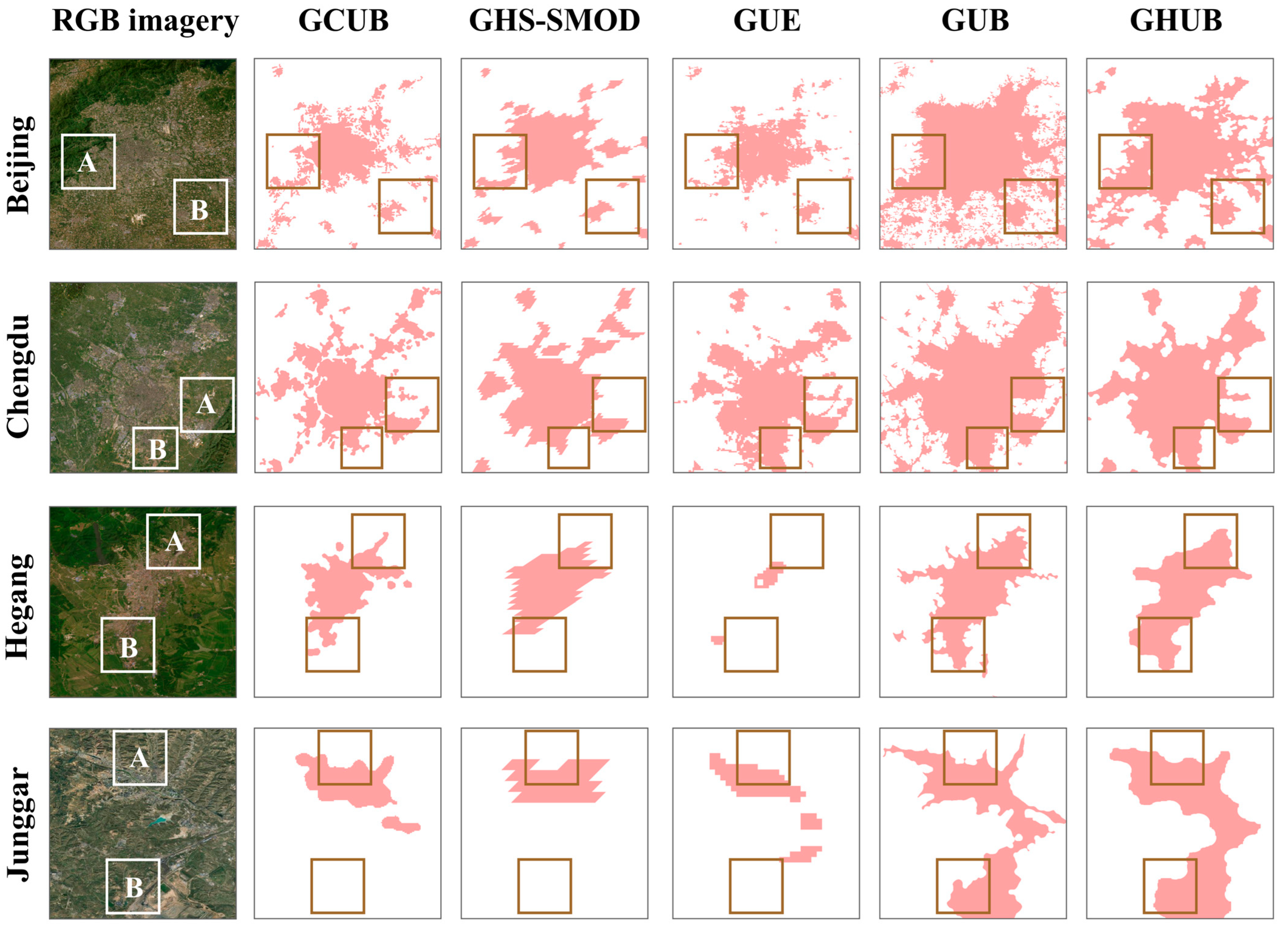
We selected four typical cities, including Beijing (the capital of China), Chengdu (one of the largest cities in Southwest China), Hegang (an RBC in Northeast China, identified by the government as a resource-depleted city), and Junggar (a county-level city under the jurisdiction of Ordos, an RBC in northwest China, home to one of Asia’s largest open-pit coal mine), to compare the visual differences in urban boundary delineation among different data products. Although all five datasets, to some extent, delineate these cities’ boundaries, there are significant differences in detail (Figure 3).

GHS-SMOD and GCUB are based on GHSL data; hence, they appear more similar in shape. However, because of the 1 km resolution of SMOD, its edges exhibit noticeable jaggedness, failing to precisely capture the detailed edges of cities and missing geographically isolated small urban patches. In the urban boundary delineation of Beijing, Chengdu, and Junggar, the shapes in GUE are relatively closer to those in GCUB and SMOD. However, the urban area in Hegang shown in GUE is significantly smaller than in the other datasets, exhibiting extensive omission. GUB and GHUB are both based on 30 m resolution impervious surface data; thus, the urban edge areas appear smoother. Visually, however, the city extents they delineate are generally larger than those of the other three data products, particularly with GUB data. For example, in Beijing, a substantial grain production base in the North China Plain, GUB incorrectly identifies a large number of surrounding rural areas as urban regions (Beijing-B). In Junggar, the Heidaigou open-pit coal mine (Junggar-B) is also mistaken by GUB and GHUB as a contiguous urban area. Similarly, in Hegang’s Lingbei open-pit coal mine (Hegang-A) and Xing’an coal mine (Hegang-B), GUB and GHUB also exhibit misclassification.

To analyze and compare the accuracy of the GCUB dataset with other datasets quantitatively, this study utilized randomly generated points, determining whether they fell within urban boundaries based on visual interpretation of high-resolution Google Maps imagery from 2020. The following strategy was employed to generate 2000 random points: (1) The union of the five datasets was taken, and a buffer zone with a radius of 2.5 km [48] was created, within which 1000 random points were generated and (2) 200 points were randomly generated within each dataset, totaling 1000 points. This approach aimed to ensure that the analysis covered each dataset’s specific characteristics and potential biases. The results (

Table 2. Confusion matrix for five datasets in 2020 and their accuracy assessments.

GCUB	Urban	Non-Urban	PA	GHS-SMOD	Urban	Non-Urban	PA
Urban	615	45	93%	Urban	564	96	85%
Non-Urban	132	1208		Non-Urban	190	1150
UA	82%			UA	75%
OA	91%	F-score	87%	OA	86%	F-score	80%
GUE	Urban	Non-Urban	PA	GUB	Urban	Non-Urban	PA
Urban	489	171	74%	Urban	647	13	98%
Non-Urban	110	1230		Non-Urban	487	853
UA	82%			UA	57%
OA	86%	F-score	78%	OA	75%	F-score	72%
				GHUB	Urban	Non-Urban	PA
				Urban	611	49	93%
				Non-Urban	379	961
				UA	62%
				OA	79%	F-score	74%

) demonstrate that GCUB, with an overall accuracy (OA) of 91%, exhibited the highest accuracy among all evaluated products. GHS-SMOD and GUE achieved slightly lower accuracies at 86%, while GUB recorded the lowest overall accuracy at 75%. GUB and GHUB excelled in producer accuracy (PA) but showed lower user accuracy (UA). This suggests that, despite these products’ ability to identify urban areas accurately, they tend to misclassify a substantial amount of non-urban areas as urban. This finding is consistent with Zhang’s conclusions [49]. Considering the imbalance in urban and non-urban sample points among the 2000 selected, an F-score was introduced as a supplementary assessment metric. The results revealed that GCUB achieved an F-score of 87%, highlighting its outstanding precision.

4.2. Spatiotemporal Characteristics of RBCs’ Urban Entities

We counted the urban entity patches marked in Step 5 over the years. During this period, both RBCs and non-RBCs saw a steady increase in urban patches, with LUPP being the main driver of this increase (Figure 4). The result indicates that over the past 20 years, numerous satellite towns formed around major cities as they urbanized. Notably, the number of LUPs declined in 2020 compared with 2015, likely because of the ongoing expansion of LUPs leading to the merging of various urban patches into larger urban clusters, a significant characteristic and trend in China’s urbanization.

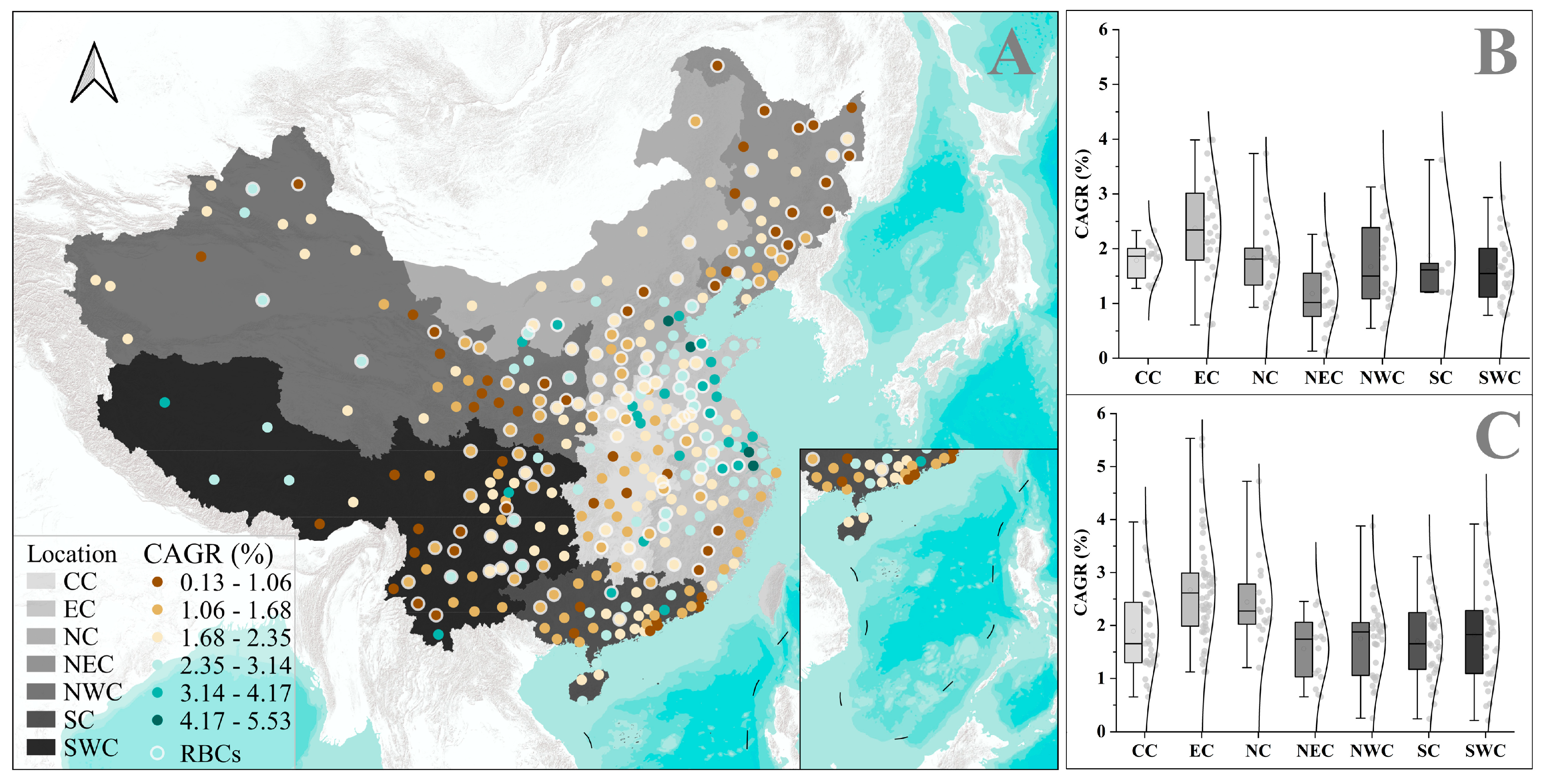
From 2000 to 2020, China’s urban area increased to 110,430.37 km². The growth in urban areas also varied geographically, as shown in Figure 5. The most significant increases in urban areas were in Eastern China for RBCs or non-RBCs. Conversely, urban areas in the Northeast lagged behind the national average, particularly for RBCs in the Northeast, with a Compound Annual Growth Rate (CAGR) of only 1.18%. Only in the south did RBCs have a slightly higher CAGR than non-RBCs, while the most significant difference between RBCs and non-RBCs was in North China, with a mean CAGR disparity of 0.62%.

4.3. Vegetation Cover Response to Urban Expansion

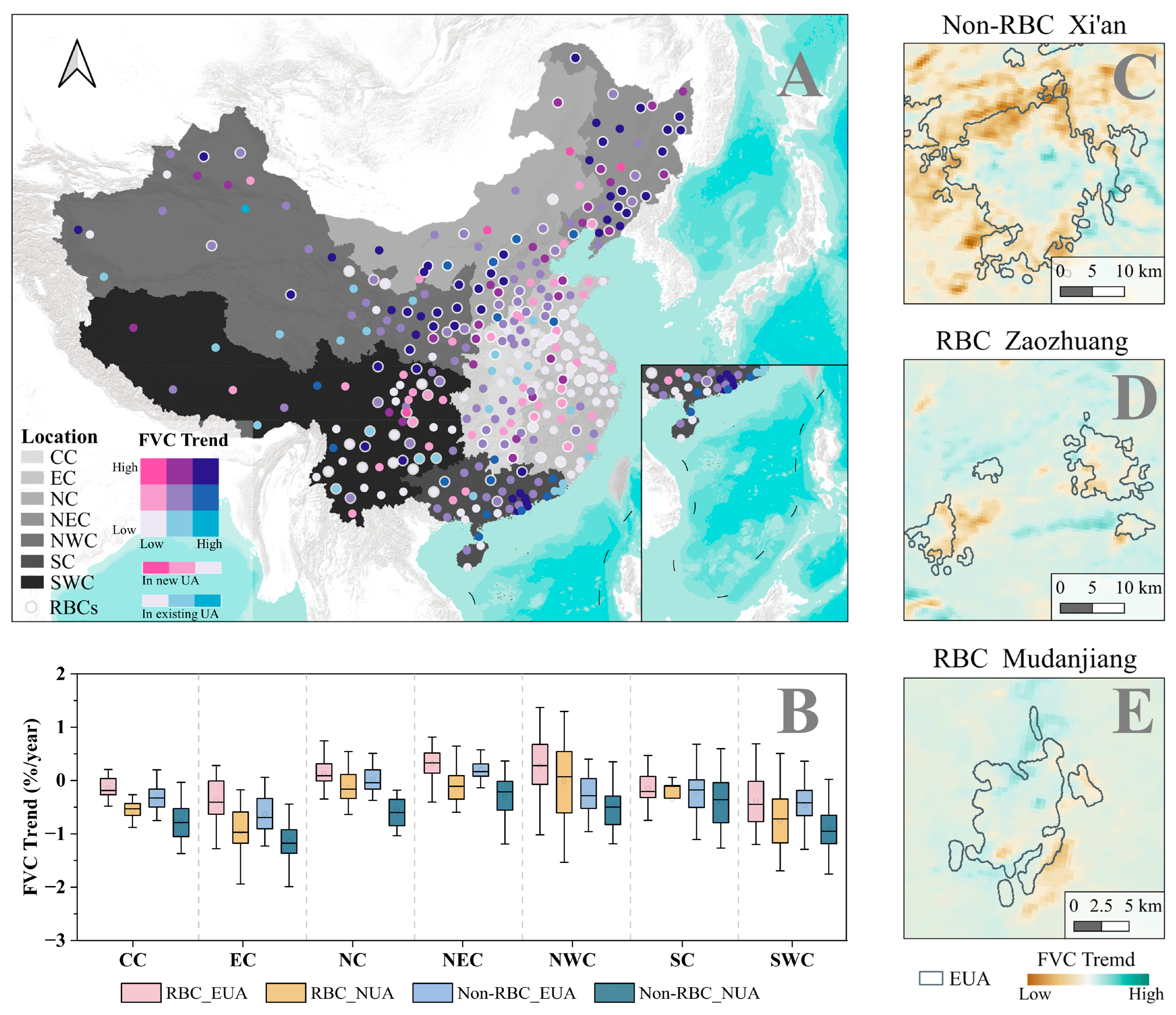
Analyzing the FVC trend distribution in the EUA and NUA, we found that a third of the cities nationwide exhibited an upward FVC trend in the EUA, while only about 50 cities showed an increasing trend in the NUA. FVC trends varied by location as follows: northern cities showed more coordination between urban expansion and greening than in the south (Figure 6). However, both RBCs and non-RBCs exhibited similar differences in various locations, with RBCs tending towards more greening or less browning, with most areas displaying an FVC trend order of RBC_EUA > Non-RBC_EUA > RBC_NUA > Non-RBC_NUA. Especially RBCs in Northwest China had an FVC trend in the EUA that was 0.52%/year higher than non-RBCs.

4.4. Resource Dependence Analysis

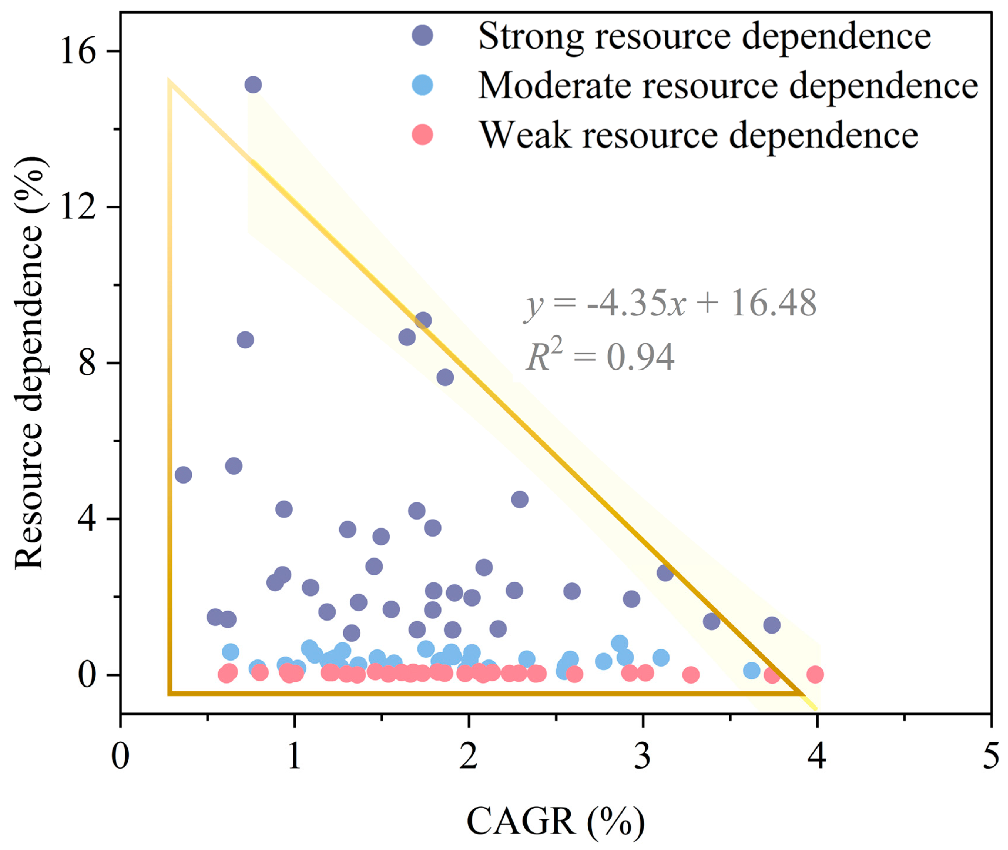
Since no new data were collected in 2020’s yearbook, we selected 2019 as the standard year, ultimately identifying the industry employment numbers in 115 RBCs to calculate the resource dependence. Statistical analysis showed that 37 cities had strong resource dependence, while 43 had moderate resource dependence. When analyzing the relationship between the type of resource dependency and GAGR, we observed that the Pearson correlation coefficient varied. The correlation coefficient for cities with weak resource dependence was −0.41, indicating a moderate negative correlation between resource dependency and GAGR. Cities with strong resource dependence showed a correlation coefficient of −0.31, also indicating a negative correlation. Moreover, cities with moderate resource dependence had a correlation coefficient of just 0.02, suggesting almost no correlation between resource dependency and GAGR. These findings indicated that varying degrees of resource dependency may impact urban growth rates differently. By plotting the relationship between urban expansion rates and resource dependency, we observed that the scatter distribution formed an approximate right-angled triangle (Figure 7). This distribution pattern suggests that there may be a trade-off and coexistence between resource dependency and urban expansion, necessitating that urban development strategies balance the two.

5. Discussion

5.1. The Relationship between the Resource Curse, Urban Expansion, and Urban Greening

Economic growth and urban expansion in China exhibit significant imbalances along the east–west axis, with cities in the east developing more rapidly [50]. Additionally, the distribution of RBCs and non-RBCs shows regional clustering, particularly with a high concentration of RBCs in the northern areas. Considering the above significant regional differences, we adopted an intra-regional comparison method to minimize the impact of regional disparities on the analysis. We conducted comparative analyses of RBCs and non-RBCs across seven regions in China. The results indicate that within the same region, the expansion rate of RBCs generally lags behind that of non-RBCs. But resource dependency does not always negatively correlate with urban development. RBCs at different stages of development show varied patterns; for instance, cities like Ordos and Karamay, which are emerging RBCs, have seen economic boosts from substantial resource production that fuel urban expansion. However, prolonged resource dependency can hinder transformation and slow expansion, as observed in cities like Jixi and Hegang. The negative correlation between resource dependency and urban development becomes more pronounced when the dependency weakens. Since implementing the Plan, some RBCs like Xuzhou and Huzhou have successfully undergone economic transformations, leading to significant urban expansion. Overall, there is a trade-off and coexistence between resource dependency and urban growth, suggesting that resource management and urban planning require more flexible and diversified strategies to promote sustainable development.

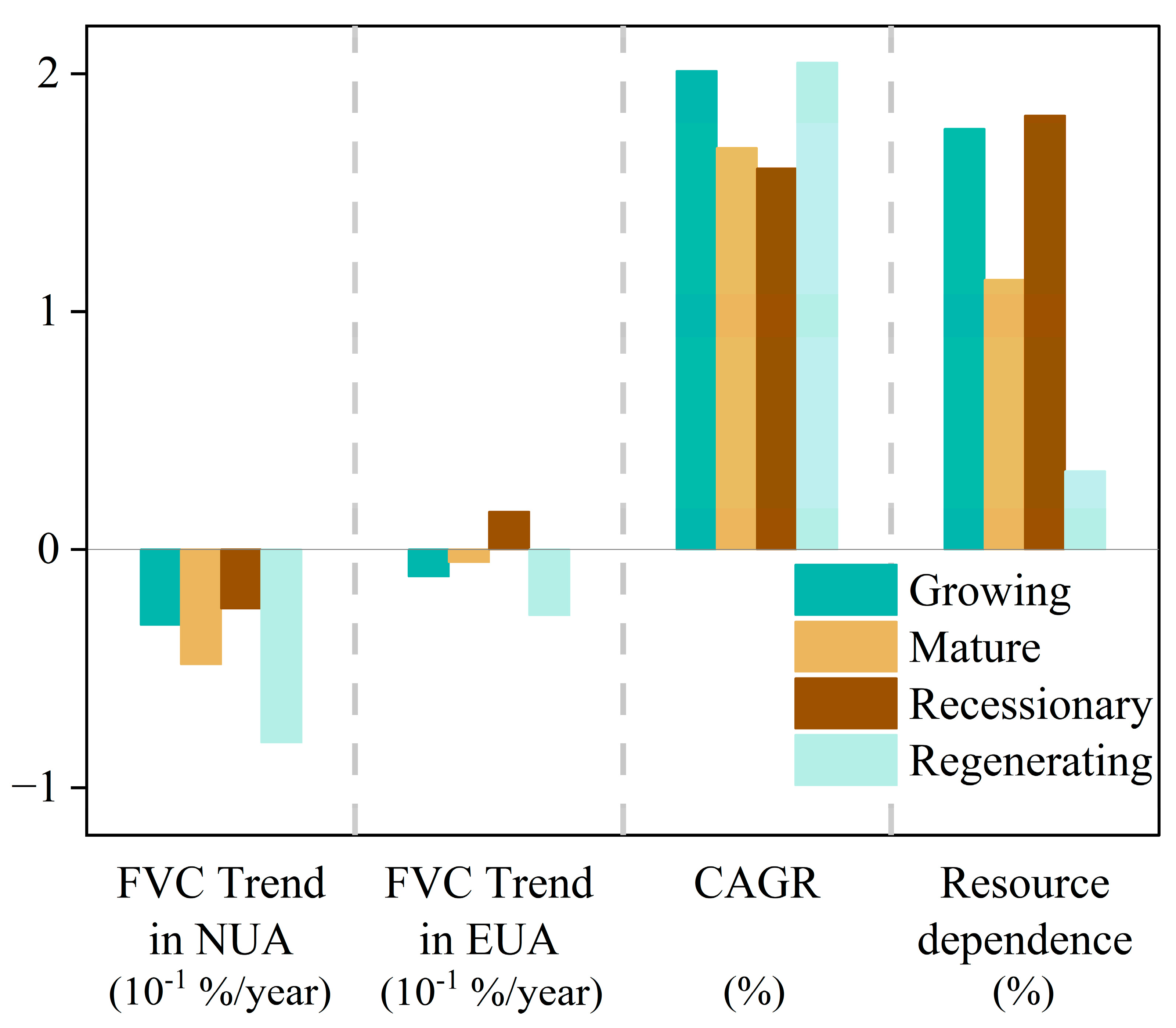
According to the Plan, China’s RBCs are categorized into four types as follows: mature (65 cities), growing (20 cities), recessionary (24 cities), and regenerating (16 cities). Several trends emerge by analyzing the average values of four key indicators, including the FVC trend in NUA, the FVC trend in EUA, CAGR, and resource dependence (Figure 8). Regenerating RBCs exhibit a higher CAGR and the lowest resource dependence, whereas recessionary RBCs show the opposite pattern. The FVC trend in NUA is negative for all four types of cities, particularly in regenerating cities, which reach −0.81%/year, followed by mature RBCs. Notably, recessionary RBCs exhibit a positive FVC trend in EUA, indicating a greening trend. These findings reveal the complex dynamics of vegetation cover change and economic transformation in RBCs.

From these observations, it can be inferred that despite the coexistence of greening and browning in urban FVC, overall urban expansion tends to decrease FVC. As regenerating cities gradually reduced their resource reliance, they experienced faster urban growth. The secondary urbanization of central areas and suburban expansion have improved land-use efficiency but have also accelerated the decline in FVC in both old and new urban areas. In contrast, recessionary RBCs still exhibit high resource dependence and currently face issues such as resource depletion and population loss, which have reduced human disturbances to urban vegetation. These cities have also increased investments in green infrastructure to address environmental problems caused by resource extraction, leading to vegetation recovery. Additionally, the low efficiency in developing new urban areas and the relatively inefficient land use in these cities result in a less pronounced decline in the FVC trend in EUA [51]. Growing RBCs present a different scenario. Despite a generally high expansion trend over 20 years, they have remained heavily dependent on resources, suggesting that future development may require strategic transformations. These observations reflect the diverse characteristics of RBCs at different development stages, highlighting the need for continued research and differentiated urban development policies even after the end of the Plan’s period [13].

5.2. Research Shortcomings and Prospects

In this study, an automated urban boundary identification method was developed based on the specific needs for urban definition and management set by the Chinese government. The thresholds set in this method are tailored to China’s specific environmental context and are relatively reliable according to accuracy analysis results. The fundamental principles of this method hold the potential for adaptation and application to urban identification in other countries following appropriate optimization. Although this study conducted visual assessments and random sample verification, the inconsistent definitions of urban boundaries across different datasets led to some uncertainties in accuracy evaluation. In light of this, future research will focus on conducting more comprehensive data quality assessments, analyzing the accuracy characteristics of different datasets in-depth, and exploring their applicability in various regions.

While the threshold settings were carefully considered to reflect the current situation in China and are theoretically supported, thresholds are inherently rigid classification tools. Because of blurred urban–rural boundaries and significant variations in urban morphology across different locations, a single threshold value cannot accurately delineate all urban boundaries [52,53]. Therefore, future research should consider employing unsupervised methods to establish adaptive thresholds. Additionally, the precision of the products generated in this study also depends on the accuracy of the GHSL data.

The urbanization of RBCs presents a complex and systemic challenge encompassing social and economic dimensions. This study primarily offers insights and data from a remote sensing perspective, providing information that is difficult to capture through conventional social statistics. However, when analyzing the impact of the resource curse on the development of RBCs, it is crucial to consider a broader array of socioeconomic indicators to elucidate the mechanisms and effects of the resource curse more scientifically. Current studies utilizing economic statistics and nighttime light remote sensing data have identified significant urban shrinkage in many RBCs [54,55]. In the next step, we will integrate this research with these data to observe urbanization in RBCs comprehensively.

6. Conclusions

This study developed an automated top-down urban boundary identification method using 100 m resolution GHS-BUILT-S and GHS-POP data, combined with the definition and characteristics of Chinese cities. Through visual comparison and random sample accuracy verification, the overall accuracy of GCUB is 91%. Based on the information on urban expansion derived from urban boundaries, we found that the resource curse is well-reflected in urban expansion. Overall, RBCs in China lag behind non-RBCs, with RBCs in Northeast China expanding the slowest and the most significant speed discrepancy between RBCs and non-RBCs observed in North China. However, greening in RBCs is notably stronger than in non-RBCs, reflecting the effectiveness of policies aimed at green transformation in RBCs.

The method proposed in this study uses only GHSL data and urban administrative boundary information, both of which are easily accessible. The delineation of urban boundaries meets the research requirements, highlighting the potential of GHSL data in urban studies. Given the method’s clear and straightforward process, it has the potential for application in other countries, though further evaluation is needed to assess the suitability of various thresholds in different regions. This study also provides a wealth of foundational data and new insights for research on urbanization in China, contributing to RBC management and sustainable development planning.

References

1. Perera, A.; Javanroodi, K.; Mauree, D.; Nik, V.; Florio, P.; Hong, T.; Chen, D. Challenges resulting from urban density and climate change for the EU energy transition. Nat. Energy 2023, 8, 397–412. [Google Scholar] [CrossRef]
2. Zhang, X.Q. The trends, promises and challenges of urbanisation in the world. Habitat. Int. 2016, 54, 241–252. [Google Scholar] [CrossRef]
3. Antonio Chaparro Torres, R.; Wang, J.; Zhang, J.; Liu, L.; Lan, Y. Temporal analysis of land degradation and urban expansion in central Yunnan Province using remote sensing for supporting sustainable development goals 11/15. Ecol. Indic. 2024, 163, 112058. [Google Scholar] [CrossRef]
4. Zhou, W.; Yu, W.; Qian, Y.; Han, L.; Pickett, S.; Wang, J.; Li, W.; Ouyang, Z. Beyond city expansion: Multi-scale environmental impacts of urban megaregion formation in China. Natl. Sci. Rev. 2022, 9, nwab107. [Google Scholar] [CrossRef] [PubMed]
5. Han, J.; Hu, Z.; Wang, P.; Yan, Z.; Li, G.; Zhang, Y.; Zhou, T. Spatio-temporal evolution and optimization analysis of ecosystem service value-A case study of coal resource-based city group in Shandong, China. J. Clean. Prod. 2022, 363, 132602. [Google Scholar] [CrossRef]
6. Badeeb, R.A.; Lean, H.H.; Clark, J. The evolution of the natural resource curse thesis: A critical literature survey. Resour. Policy 2017, 51, 123–134. [Google Scholar] [CrossRef]
7. van der Ploeg, F. Natural Resources: Curse or Blessing? J. Econ. Lit. 2011, 49, 366–420. [Google Scholar] [CrossRef]
8. Cao, Y.; Kong, L.; Zhang, L.; Ouyang, Z. The balance between economic development and ecosystem service value in the process of land urbanization: A case study of China’s land urbanization from 2000 to 2015. Land Use Policy 2021, 108, 105536. [Google Scholar] [CrossRef]
9. Wang, Y.; Chen, H.; Long, R.; Sun, Q.; Jiang, S.; Liu, B. Has the Sustainable Development Planning Policy Promoted the Green Transformation in China’s Resource-based Cities. Resour. Conserv. Recycl. 2022, 180, 106181. [Google Scholar] [CrossRef]
10. Wen, S.; Jia, Z. Resource curse or resource blessing: Perspective on the nonlinear and regional relationships in China. J. Clean. Prod. 2022, 371, 133491. [Google Scholar] [CrossRef]
11. Cheng, Z.; Li, X.; Wang, M. Resource curse and green economic growth. Resour. Policy 2021, 74, 102325. [Google Scholar] [CrossRef]
12. Liu, Q.; Li, F.; Peng, L.; Dong, S.; Yang, Y.; Cheng, H. Multiple evaluation framework of sustainability development in resource-based cities: A case study of China. Ecol. Indic. 2024, 158, 111338. [Google Scholar] [CrossRef]
13. Li, W.; Cai, Z.; Jin, L. Urban green land use efficiency of resource-based cities in China: Multidimensional measurements, spatial-temporal changes, and driving factors. Sust. Cities Soc. 2024, 104, 105299. [Google Scholar] [CrossRef]
14. Wang, Y.; Wang, W.; Shen, C.; Li, W. End of rope or phoenix nirvana? Exploring the evolutionary paths of coal resource-based cities in China. Cities 2024, 154, 105382. [Google Scholar] [CrossRef]
15. Alvioli, M. Administrative boundaries and urban areas in Italy: A perspective from scaling laws. Landsc. Urban. Plan. 2020, 204, 103906. [Google Scholar] [CrossRef] [PubMed]
16. Wang, H.; Ning, X.; Zhang, H.; Liu, Y. Urban expansion analysis of China’s prefecture level city from 2000 to 2016 using high-precision urban boundary. In Proceedings of the 2019 IEEE International Geoscience and Remote Sensing Symposium (IGARSS 2019), Yokohama, Japan, 28 July–2 August 2019; pp. 7514–7517. [Google Scholar]
17. Richards, D.; Belcher, R. Global Changes in Urban Vegetation Cover. Remote Sens. 2020, 12, 23. [Google Scholar] [CrossRef]
18. Harig, O.; Hecht, R.; Burghardt, D.; Meinel, G. Automatic Delineation of Urban Growth Boundaries Based on Topographic Data Using Germany as a Case Study. ISPRS Int. J. Geo-Inf. 2021, 10, 353. [Google Scholar] [CrossRef]
19. He, X.; Zhu, Y.; Chang, P.; Zhou, C. Using Tencent User Location Data to Modify Night-Time Light Data for Delineating Urban Agglomeration Boundaries. Front. Environ. Sci. 2022, 10, 860365. [Google Scholar] [CrossRef]
20. Hu, S.; Tong, L.; Frazier, A.E.; Liu, Y. Urban boundary extraction and sprawl analysis using Landsat images: A case study in Wuhan, China. Habitat. Int. 2015, 47, 183–195. [Google Scholar] [CrossRef]
21. Li, J.; Huang, X. Impact of land-cover layout on particulate matter 2.5 in urban areas of China. Int. J. Digit. Earth 2020, 13, 474–486. [Google Scholar] [CrossRef]
22. Yao, L. Assessment of long time-series greening signatures across the urban–rural gradient in Chinese cities. Ecol. Indic. 2024, 160, 111826. [Google Scholar] [CrossRef]
23. Zhou, D.; Zhao, S.; Liu, S.; Zhang, L.; Zhu, C. Surface urban heat island in China’s 32 major cities: Spatial patterns and drivers. Remote Sens. Environ. 2014, 152, 51–61. [Google Scholar] [CrossRef]
24. Florczyk, A.; Melchiorri, M.; Corbane, C.; Schiavina, M.; Pesaresi, M.; Politis, P. Description of the GHS Urban Centre Database 2015; Publications Office of the European Union: Luxembourg, 2019. [Google Scholar]
25. Li, X.; Gong, P.; Zhou, Y.; Wang, J.; Bai, Y.; Chen, B.; Hu, T.; Xiao, Y.; Xu, B.; Yang, J.; et al. Mapping global urban boundaries from the global artificial impervious area (GAIA) data. Environ. Res. Lett. 2020, 15, 094044. [Google Scholar] [CrossRef]
26. Hafner, S.; Ban, Y.; Nascetti, A. Unsupervised domain adaptation for global urban extraction using Sentinel-1 SAR and Sentinel-2 MSI data. Remote Sens. Environ. 2022, 280, 113192. [Google Scholar] [CrossRef]
27. Pesaresi, M.; Maffenini, L.; Freire, S.; Politis, P.; Schiavina, M. GHS-SDATA R2023A—GHS Supporting Data; Joint Research Centre (JRC): Brussels, Belgium, 2023. [Google Scholar]
28. Uhl, J.H.; Leyk, S. A scale-sensitive framework for the spatially explicit accuracy assessment of binary built-up surface layers. Remote Sens. Environ. 2022, 279, 113117. [Google Scholar] [CrossRef]
29. Leyk, S.; Uhl, J.; Balk, D.; Jones, B. Assessing the accuracy of multi-temporal built-up land layers across rural-urban trajectories in the United States. Remote Sens. Environ. 2018, 204, 898–917. [Google Scholar] [CrossRef] [PubMed]
30. Freire, S.; Schiavina, M.; Florczyk, A.; MacManus, K.; Pesaresi, M.; Corbane, C.; Borkovska, O.; Mills, J.; Pistolesi, L.; Squires, J.; et al. Enhanced data and methods for improving open and free global population grids: Putting ‘leaving no one behind’ into practice. Int. J. Digit. Earth 2020, 13, 61–77. [Google Scholar] [CrossRef]
31. Singh, N.; Dey, S.; Knibbs, L. Spatio-temporal patterns of tropospheric NO2 over India during 2005–2019. Atmos. Pollut. Res 2023, 14, 101692. [Google Scholar] [CrossRef]
32. Vermote, E.; Wolfe, R. MOD09GA MODIS/Terra Surface Reflectance Daily L2G Global 1km and 500m SIN Grid V006; NASA Eosdis Land Processes Distributed Active Archive Center: Sioux Falls, SD, USA, 2015. [Google Scholar]
33. Shi, K.; Wu, Y.; Liu, S.; Chen, Z.; Huang, C.; Cui, Y. Mapping and evaluating global urban entities (2000–2020): A novel perspective to delineate urban entities based on consistent nighttime light data. Gisci. Remote Sens. 2023, 60, 2161199. [Google Scholar] [CrossRef]
34. Xu, Z.; Jiao, L.; Lan, T.; Zhou, Z.; Cui, H.; Li, C.; Xu, G.; Liu, Y. Mapping hierarchical urban boundaries for global urban settlements. Int. J. Appl. Earth Obs. Geoinf. 2021, 103, 102480. [Google Scholar] [CrossRef]
35. Wang, N.; Zhang, X.; Yao, S.; Wu, J.; Xia, H. How Good Are Global Layers for Mapping Rural Settlements? Evidence from China. Land. 2022, 11, 1308. [Google Scholar] [CrossRef]
36. Uhl, J.H.; Leyk, S. Spatially explicit accuracy assessment of deep learning-based, fine-resolution built-up land data in the United States. Int. J. Appl. Earth Obs. Geoinf. 2023, 123, 103469. [Google Scholar] [CrossRef] [PubMed]
37. Corbane, C.; Syrris, V.; Sabo, F.; Politis, P.; Melchiorri, M.; Pesaresi, M.; Soille, P.; Kemper, T. Convolutional neural networks for global human settlements mapping from Sentinel-2 satellite imagery. Neural Comput. Appl. 2021, 33, 6697–6720. [Google Scholar] [CrossRef]
38. Zhou, D.; Zhao, S.; Zhang, L.; Liu, S. Remotely sensed assessment of urbanization effects on vegetation phenology in China’s 32 major cities. Remote Sens. Environ. 2016, 176, 272–281. [Google Scholar] [CrossRef]
39. Imhoff, M.L.; Zhang, P.; Wolfe, R.E.; Bounoua, L. Remote sensing of the urban heat island effect across biomes in the continental USA. Remote Sens. Environ. 2010, 114, 504–513. [Google Scholar] [CrossRef]
40. Zhou, Y.; Shi, Y. Toward establishing the concept of physical urban area in China. Acta Geogr. Sin. 1995, 4, 289–301. [Google Scholar]
41. Dijkstra, L.; Brandmüller, T.; Kemper, T.; Khan, A.A.; Veneri, P. Applying the Degree of Urbanisation: A Methodological Manual to Define Cities, Towns and Rural Areas for International Comparisons; OECD: Paris, France, 2021. [Google Scholar]
42. Wang, R.; Han, R.; Chen, Y. Key technical issues in the application of the code of practice for standard urban built-up area delineation. City Plan. Rev. 2024, 1–7. [Google Scholar]
43. Wu, C.; Murray, A.T. Estimating impervious surface distribution by spectral mixture analysis. Remote Sens. Environ. 2003, 84, 493–505. [Google Scholar] [CrossRef]
44. Su, Y.; Wang, D.; Zhao, S.; Shi, J.; Shi, Y.; Wei, D. Examining long-term natural vegetation dynamics in the Aral Sea Basin applying the linear spectral mixture model. PeerJ 2021, 9, e10747. [Google Scholar] [CrossRef]
45. Camps-Valls, G.; Campos-Taberner, M.; Moreno-Martínez, A.; Walther, S.; Duveiller, G.; Cescatti, A.; Mahecha, M.; Muñoz-Marí, J.; García-Haro, F.; Guanter, L.; et al. A unified vegetation index for quantifying the terrestrial biosphere. Sci. Adv. 2021, 7, eabc7447. [Google Scholar] [CrossRef]
46. Wu, S.; Chen, B.; Webster, C.; Xu, B.; Gong, P. Improved human greenspace exposure equality during 21st century urbanization. Nat. Commun. 2023, 14, 6460. [Google Scholar] [CrossRef] [PubMed]
47. Yan, T.; Hu, Y. Classification of resource-based cities from the perspective of resource decoupling. Resour. Sci. 2019, 41, 2172–2181. [Google Scholar] [CrossRef]
48. Tao, Y.; Liu, W.; Chen, J.; Gao, J.; Li, R.; Ren, J.; Zhu, X. A Self-Supervised Learning Approach for Extracting China Physical Urban Boundaries Based on Multi-Source Data. Remote Sens. 2023, 15, 3189. [Google Scholar] [CrossRef]
49. Zhang, X.; Du, S.; Zhou, Y.; Xu, Y. Extracting physical urban areas of 81 major Chinese cities from high-resolution land uses. Cities 2022, 131, 104061. [Google Scholar] [CrossRef]
50. Yin, C.; Meng, F.; Yang, X.; Yang, F.; Fu, P.; Yao, G.; Chen, R. Spatio-temporal evolution of urban built-up areas and analysis of driving factors—A comparison of typical cities in north and south China. Land. Use Policy 2022, 117, 106114. [Google Scholar] [CrossRef]
51. He, T.; Song, H. A novel approach to assess the urban land-use efficiency of 767 resource-based cities in China. Ecol. Indic. 2023, 151, 110298. [Google Scholar] [CrossRef]
52. Alexander Wandl, D.I.; Nadin, V.; Zonneveld, W.; Rooij, R. Beyond urban–rural classifications: Characterising and mapping territories-in-between across Europe. Landsc. Urban. Plan. 2014, 130, 50–63. [Google Scholar] [CrossRef]
53. Urso, G. Metropolisation and the challenge of rural-urban dichotomies. Urban. Geogr. 2021, 42, 37–57. [Google Scholar] [CrossRef]
54. Han, J.; Hu, Z.; Sajadi, P.; Li, S.; Zhang, Y.; Cui, R.; Pilla, F. Evaluating urban development in China’s resource-based cities: A new perspective using nighttime light data. Int. J. Digit. Earth 2024, 17, 2349747. [Google Scholar] [CrossRef]
55. He, T.; Song, H.; Chen, W. Recognizing the transformation characteristics of resource-based cities using night-time light remote sensing data: Evidence from 126 cities in China. Resour. Policy 2023, 85, 104013. [Google Scholar] [CrossRef]
Figure 1. Distribution of RBCs in China and the geographic divisions of China. (CC: Central China; EC: East China; NC: North China; NEC: Northeast China; NWC: Northwest China; SC: South China; SWC: Southwest China).
Remotesensing 16 03640 g001
Figure 2. Flowchart of the adopted methodology for mapping GCUB.
Remotesensing 16 03640 g002
Figure 3. Comparison of GCUB with other urban boundary datasets in different cities, including Beijing, Chengdu, Hegang, and Junggar.
Remotesensing 16 03640 g003
Figure 4. Trends in the expansion and number of urban patches in China from 2000 to 2020. (A): Overall statistics of China. (B): Statistics of RBCs.
Remotesensing 16 03640 g004
Figure 5. The CAGR and its distribution of RBCs and non-RBCs. (A): The distribution map of the CAGR of urban areas across cities in China (classified based on natural breaks method). (B): Regional statistics of CAGR for RBCs. (C): Regional statistics of the CAGR for non-RBCs.
Remotesensing 16 03640 g005
Figure 6. FVC trends within the EUA and NUA across different regions. (A): Distribution of the FVC trend across cities. (B): Spatial statistics of the FVC trend. (CE): City examples.
Remotesensing 16 03640 g006
Figure 7. The scatter plot of resource dependency and GAGR for RBCs forming an approximate right-angled triangle shape.
Remotesensing 16 03640 g007
Figure 8. Values of four indicators across different development categories of RBCs.
Remotesensing 16 03640 g008