1. Introduction
Remote sensing change detection refers to the technique of using remote sensing images of the same location from different periods to identify differences in surface entities or phenomena [
1]. Specifically, change detection is a pixel-to-pixel task that takes two temporal images as the input and predicts the location of the change occurrence [
2]. Utilizing satellite remote sensing for a multi-temporal observation of the Earth’s surface and automatic change detection provides an important technique for understanding the continuous changes on the Earth’s surface. It also significantly contributes to various fields of remote sensing applications, such as agricultural surveys, urban expansion, resource exploration, ecological assessment, and disaster monitoring [
3]. Therefore, for specific applications and tasks, designing change detection techniques with strong interpretability, high robustness, high automation, and high accuracy by fully considering spectral changes and introducing more object–semantic–geoscience knowledge support is crucial for effectively discovering, identifying, and describing surface features, which is of great significance.
Traditional change detection methods identify land cover and land use changes by analyzing the differences between image pairs. Among these, algorithms incorporating clustering or threshold segmentation and extracting manually designed spatiotemporal features have been mainstream methods [
4,
5]. These include wavelet transforms [
6,
7], a gray-level co-occurrence matrix [
8], and morphological feature extraction and analysis [
9,
10], among others. These traditional change detection algorithms heavily rely on manually designed feature selection and extraction, resulting in excessive effort spent on developing features for buildings or other objects in different scenarios, leading to inefficient workflows, labor-intensive processes, and a generally poor robustness of the models [
11], limiting their applicability in generalization.
With the rapid advancements in deep learning algorithms within the domain of computer vision [
12], remote sensing change detection has experienced a paradigm shift from traditional data-driven methods to model-driven approaches. This transition highlights the evolution from classical algorithms to sophisticated, intelligent algorithms designed to enhance change detection accuracy. Modern methods leverage various network architectures and cutting-edge deep learning techniques to address challenges specific to change detection applications [
13]. Notable architectures include convolutional neural networks (CNN) [
14], Siamese Residual Networks [
15], PGA-SiamNet [
16], cross-layer convolutional neural networks [
17], and Pure Transformer Networks [
18]. Additionally, advancements have been made with efficient modules, such as Recurrent Neural Networks (RNN) [
19], attention mechanisms [
20], and global perception modules [
21], contributing to improved accuracy in change detection.
Recent developments in remote sensing change detection models include several innovative approaches. The Dual-Task Constrained Deep Siamese Convolutional Network [
22] combines change detection and semantic segmentation tasks through dual attention modules and enhanced loss functions, which significantly improve the extraction of critical change features. However, this model’s data-driven nature necessitates extensive training data, leading to high computational costs. Conversely, methods utilizing spatiotemporal attention have introduced datasets like the LEVIR-CD and leverage self-attention mechanisms to capture spatiotemporal dependencies, thereby offering more refined feature representations for change detection. However, these methods often struggle with a monotonic representation of spatiotemporal relationships, lacking diversity and robustness. The Big Transfer (BiT) method, which enhances visual representation learning through large-scale pretraining and transfer learning, is instrumental in deriving general feature representations from remote sensing images [
23]. However, the large size of pretrained models can limit their use in resource-constrained environments.
The ChangeFormer model [
24], built on transformer-based Siamese networks, utilizes multi-scale long-range details to provide a precise framework for remote sensing image change detection. Similarly, the TINYCD model [
25] demonstrates improvements in change detection performance through spatial–semantic attention mechanisms while maintaining a lightweight design. However, both models may face limitations in extremely complex scenes. The Changer architecture [
2] emphasizes the role of feature interaction through interaction layers in the feature extractor, highlighting its importance in improving change detection performance. Meanwhile, the classical UNet [
26] has shown exceptional performance in practical applications, prompting researchers to extend and adapt the UNet structure for change detection with homogeneous images [
27].
To address the challenges of low semantic recognition accuracy in remote sensing image change detection, particularly for objects with complex shapes and coarse comparisons, a fine-grained high-resolution remote sensing image change detection model incorporating the Segment Anything Model (SAM), termed the SAM-UNet Change Detection Model (SCDM), is proposed. The motivation behind constructing the SCDM lies in two aspects: first, integrating the SAM encoder with the UNet network to extract features from 2D images and discover differences between comparative images through a feature space metric, thereby enhancing the accuracy of the change detection model; second, by employing fine-grained metric learning methods to improve the accuracy of pixel-level difference detection in change comparison algorithms, thereby further enhancing the accuracy of change detection. These are contributions of this study:
- (1)
We introduce the SCDM, combining the center expansion and reduction method (CERM), the Segment Anything Model (SAM), UNet, and a fine-grained loss function for enhanced building change detection.
- (2)
We incorporate the Global Feature Extractor (GFE), feature space metric evaluation module (FM), Global and Differential Feature Fusion Module (GDF), and Global Decoder Module (GD) to improve feature extraction and change detection accuracy.
- (3)
It demonstrates superior performance over traditional methods and existing models (e.g., ChangeFormer, ChangerEx) on the WHU-CD and LEVIR-CD datasets.
- (4)
Generalization experiments were carried out on the DTX dataset, representing varying resolutions, spectral features, and geographic contexts.
- (5)
Finally, a detailed inference speed test and computation evaluation are carried out, showing the proposed SCDM having high efficiency.
3. Methodology
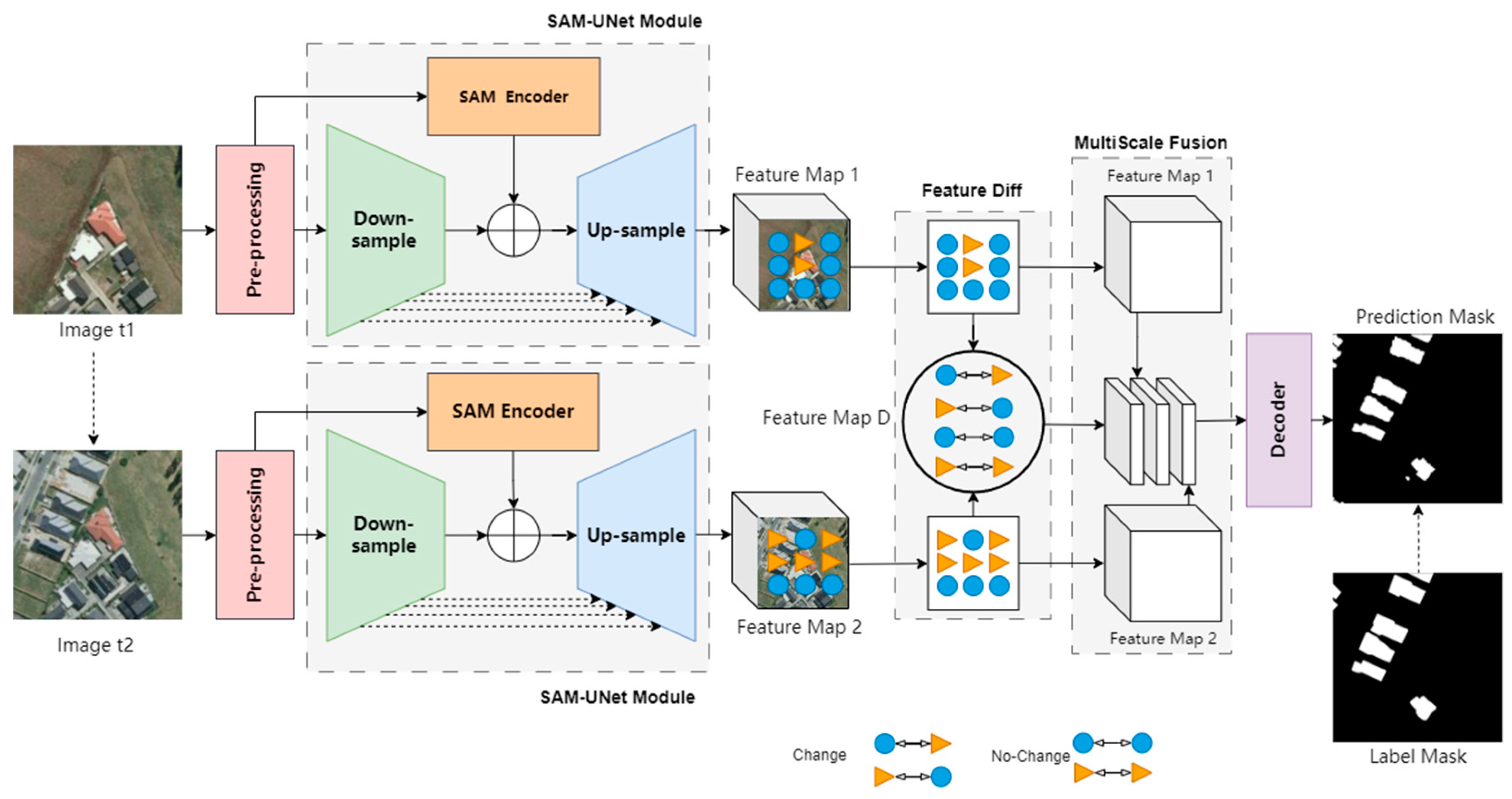
In this study, a novel framework named SCDM was proposed, as is illustrated in
Figure 3, comprising network modules including SAM and UNet. More importantly, new modules were designed for better feature extraction in the second half of SCDM: Global Feature Extractor (GFE), feature space metric evaluation module (FM), Global and Differential Feature Fusion Module (GDF), and Global Decoder Module (GD). The following will provide a detailed explanation of the image change detection model framework, integrating SAM and UNet according to the connectivity sequence of each network module.
The SCDM framework designed in this study is illustrated in
Figure 3 and consisted of several modules, including preprocessing, SAM-UNet feature extraction, feature difference comparison, multi-scale feature fusion, and a decoder. The following sections will provide a detailed introduction to the image change detection model framework that integrates SAM and UNet, organized according to the sequence of connections among the modules.
3.1. Preprocess
For the input of remote sensing images, initial preprocessing was conducted as shown in
Figure 3 (preprocessing). The preprocessing stage consisted of a 3 × 3 Conv2d convolution operation, BatchNorm2d normalization, and a ReLU activation function. The 3 × 3 Conv2d convolution operation filtered the image using a 3 × 3 kernel to extract features across various scales and orientations. BatchNorm2d normalization aided in stabilizing the training process by accelerating convergence and enhancing the model’s generalization capabilities. Lastly, the
activation function introduced non-linearity, further augmenting the expressive power of the features.
Within the designated monitoring area, images from time , denoted as , and , denoted as , along with their corresponding label data, were processed through the feature preprocessor (preprocessing). This yielded the preprocessed features .
3.2. SAM-UNet Feature Extraction
Following preprocessing, the process entered the SAM-UNet feature extraction module (as shown in
Figure 3, SAM-UNet Module), which was designed to extract global feature maps containing information about physical environmental boundaries and categories. This module will be detailed below.
For the regional image at time
, as illustrated in the upper part of the SAM-UNet module in
Figure 3, the SAM Encoder employed a pretrained VisionTransformer network structure to encode features of preprocessed building images, capturing boundary features.
In the lower part of the SAM-UNet module, the UNet backbone’s down-sampling module, Down-sample, was realized through four levels of 2 × 2 MaxPool pooling operations to acquire category features. Conversely, the up-sampling module, Up-sample, utilized an FPN (Feature Pyramid Network) structure where each level of up-sampling and down-sampling was fused with feature maps of the same resolution. This resulted in the global feature map
for the regional image at time
(shown as Feature Map 1 in
Figure 3) and, similarly,
for time (Feature Map 2 in
Figure 3).
By integrating with U-Net, the SAM Encoder effectively leveraged the image’s contextual information. This was due to the skip connections that allowed for the decoder to access high-resolution features of buildings from earlier layers, which were critical for understanding local areas of the image. Thus, even in the presence of similar textures or blurred boundaries within the image, the model can distinguish between different objects and backgrounds. The structure of U-Net focused the network’s learning on areas with greater errors. High-resolution features provided by skip connections participated directly in the generation of the final segmentation map, meaning gradients propagated directly within the network, avoiding the common problem of gradient vanishing in deep networks. This design not only enhanced the training efficiency of the network but also improved the model’s capability to capture small objects and details.
3.3. Feature Difference Comparison
When dealing with time-series image data, detecting subtle changes is often challenging, especially when changes are minute or when the data contain significant noise. In traditional feature difference detection methods, the accumulation of errors and loss of information can lead to inaccurate change detection. To address this issue, this study introduced a Feature Difference Module designed to extract the differential features of the same target before and after a temporal change (see
Figure 3, Feature Diff). Specifically, a fine-grained contrastive loss function based on the cosine distance measurement method was constructed. By comparing the global feature maps
and
from two time points, this function inferred the feature differences in the changed areas, extracting the differential features
(depicted in
Figure 3 as Feature Map D). The detailed process is outlined below.
Initially, the mathematical formula for the cosine distance function
is as follows:
where
and
represent the feature vectors of the global feature maps
and
, respectively. Furthermore, assuming the variable
represents whether there is a change in the pixel area (0 indicating no change and 1 indicating a change), the calculation formula is as follows:
where
is the cosine distance between the feature vectors of
and
computed using Equation (1);
is a manually set threshold distance.
Finally, the fine-grained contrastive loss function
can be defined as follows:
where
is a weighting factor,
;
represents the maximum distance limit for
.
According to the equation of
, the greater the feature difference and feature distance, the higher the value of the contrastive loss function. Through the comparison of feature differences, the differential feature map
can be extracted as follows:
where
and
are the global feature maps from two timestamps.
3.4. Multi-Scale Feature Fusion
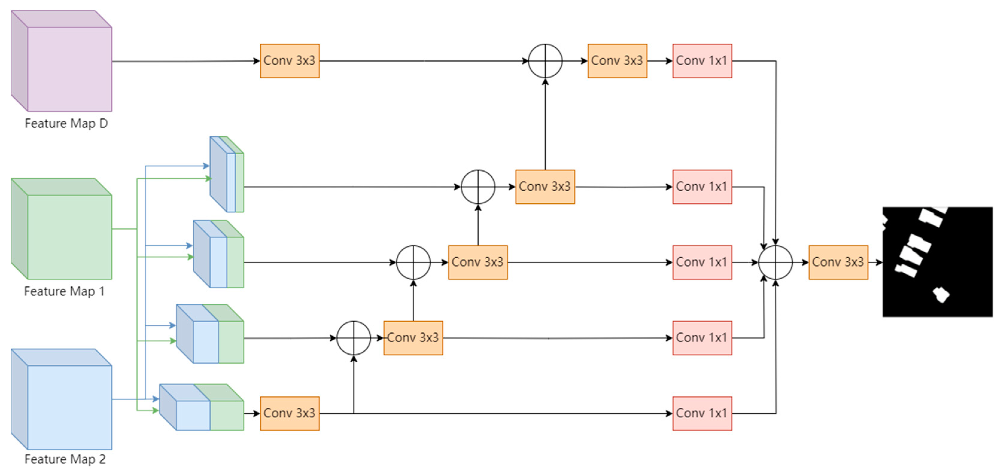
To enhance the accuracy and robustness of building change detection tasks under varying conditions, this study designed and implemented a multi-scale feature fusion module specifically for integrating global feature maps from different time points with difference features. As shown in
Figure 4, the global feature maps
each undergo a process of four levels of down-sampling and four levels of up-sampling, facilitated by a Feature Pyramid Network (FPN) architecture. This structure not only elevates the diversity of feature scales but also ensures comprehensiveness and depth of information.
After the global feature maps are down-sampled, a meticulously designed cross-fusion operation promotes the effective integration of multi-scale architectural information. This cross-fusion strategy, based on the complementarity of information, enhances the model’s capability to recognize features across different scales, enabling it to capture building change details from coarse to fine resolutions. Subsequently, these processed features undergo four levels of up-sampling through the FPN pyramid structure to increase their resolution, gradually approximating the original size for better integration with the difference feature map . This fusion process is critical, as it combines global contextual information with local detail information, significantly enhancing the model’s ability to perceive and interpret building changes. Through this deep fusion, the model adeptly identifies and annotates the areas of change in buildings without losing critical spatial and shape information.
3.5. Decoder
During the encoding phase, the dimensions and resolution of feature maps are often reduced to extract more abstract information, which may result in the loss of some detailed information. To address this issue, the SCDM designed a novel encoder (shown as Encoder in
Figure 3), tasked with predicting changes in the same region over different periods. In this process, the feature maps produced by the feature fusion module were fed into this encoder, containing crucial information from the input images, such as texture, shape, and edges. In the encoder, these feature maps underwent a series of up-sampling steps to restore them to the same resolution as the original image. This restoration was critical for ensuring that the details and texture information of the images were accurately recovered, especially in change detection, where capturing details can greatly affect the accuracy of the final results.
Following this, the features underwent further processing through a series of 3 × 3 convolution blocks designed to extract features and enhance representational power, thus better capturing subtle changes in the change regions. After processing through a Softmax function, which assigned category labels to each pixel, the final predictions regarding the change regions were obtained. These predictions not only provided information about changes in the same area at different times but were also useful for further analysis and decision-making.
4. Results and Discussions
4.1. Dataset and Preprocessing
4.1.1. Datasets
To evaluate the performance of the proposed SCDM method in this paper, remote sensing image datasets with diverse features and scenes were utilized. Specifically, the LEVIR-CD [
32] and WHU-CD [
33] open-access datasets were chosen, and a series of experiments were conducted on these datasets. The following provides an introduction to these two datasets.
The LEVIR-CD [
32] is a large-scale remote sensing dataset for building change detection, as illustrated in
Figure 5. It comprises 637 pairs of very-high-resolution (VHR, 0.5 m/pixel) Google Earth image patches, each with a size of 1024 × 1024 pixels. These dual-temporal images span a time interval of 5 to 14 years, depicting significant land use changes, particularly in building growth.
The LEVIR-CD dataset encompasses various types of buildings, such as villas, high-rise apartments, small garages, and large warehouses. The dataset focuses on changes related to buildings, including building growth (changes from soil/grass/hardened surfaces or under construction buildings to newly constructed areas) and building decay. These dual-temporal images are annotated by remote sensing image interpretation experts using binary labels (1 indicating change, 0 indicating no change), comprising a total of 31,333 individual instances of changed buildings (as depicted in
Figure 6).
The WHU-CD dataset [
33] is a remote sensing image change detection dataset created by the Sensing Intelligence, Geoscience, and Machine Learning Lab (SIGMA) at Wuhan University, introduced by Liu et al. [
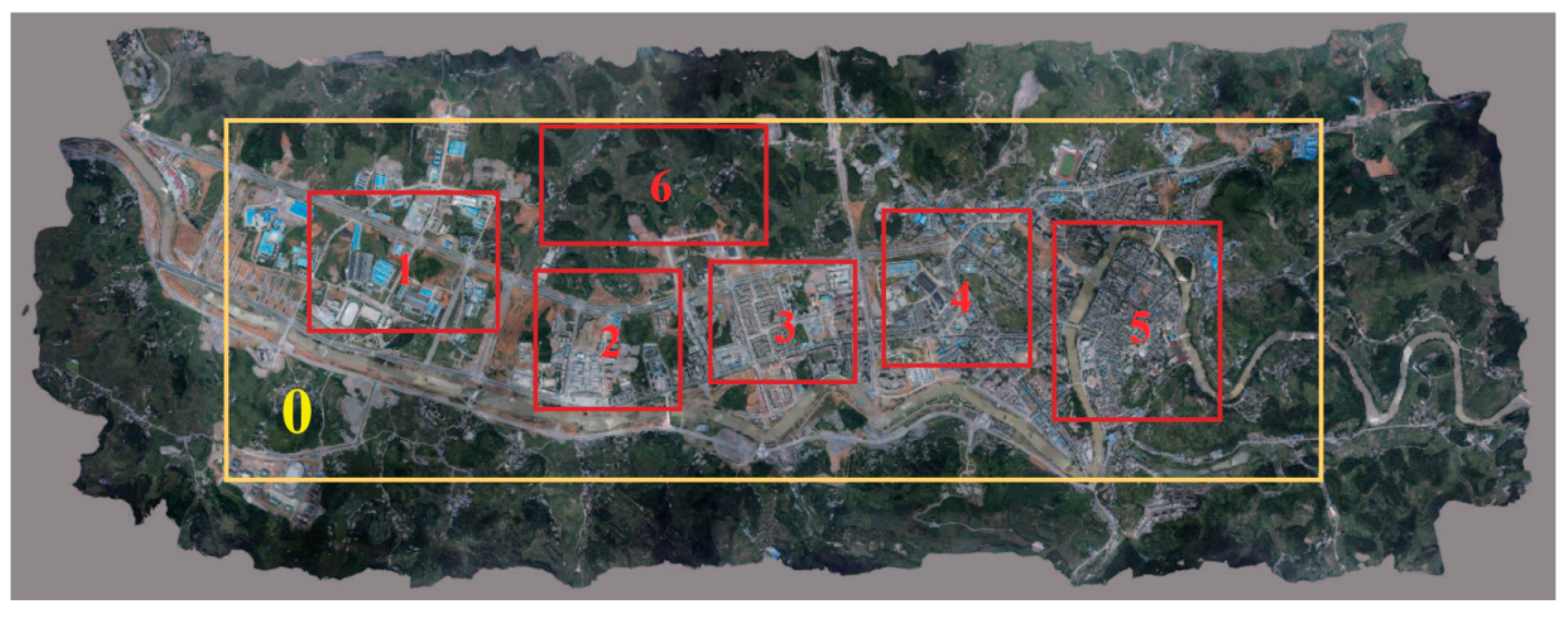
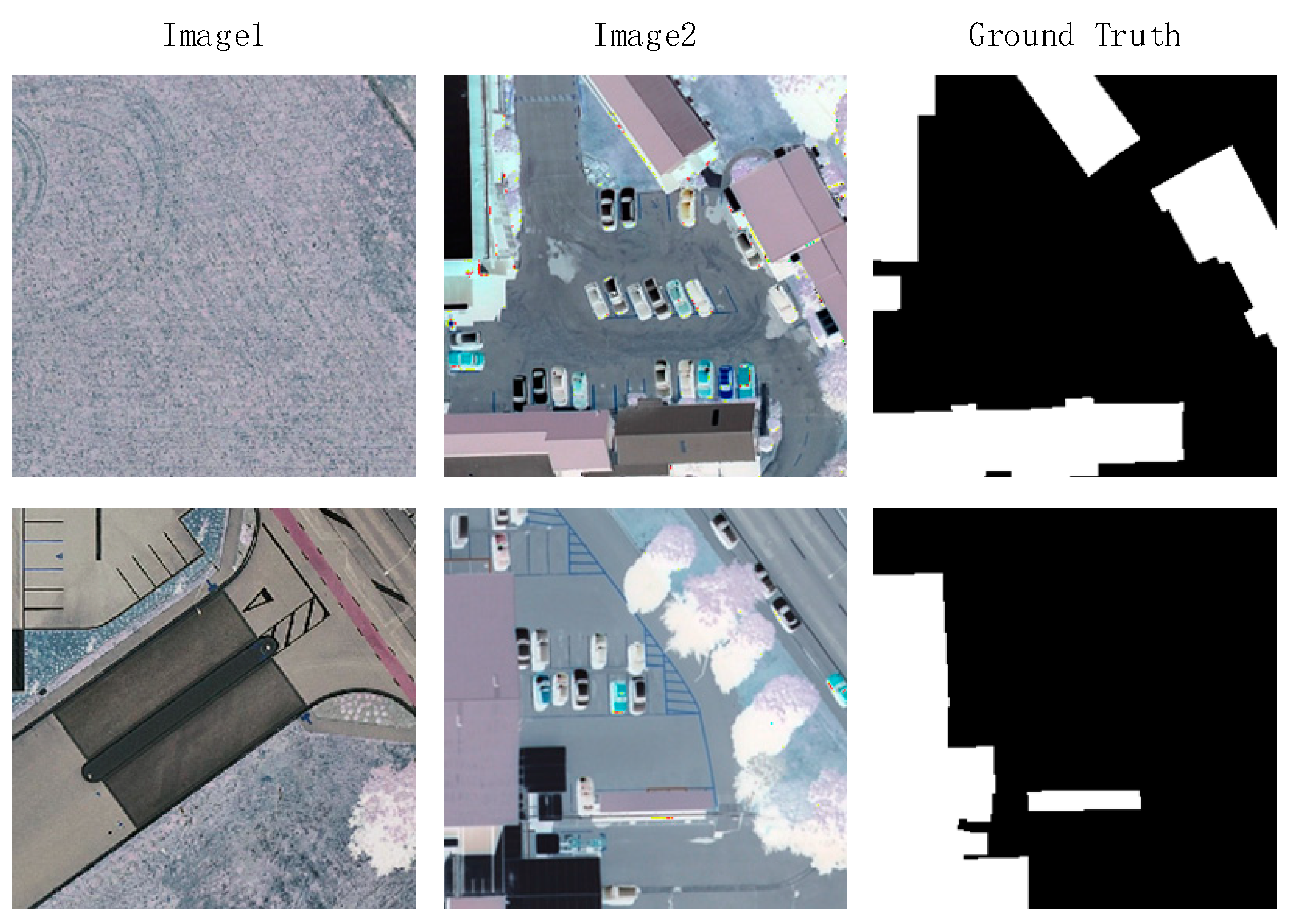
34]. This dataset comprises a pair of aerial images captured in the same area at two time points in 2012 and 2016. The image dimensions are 32,507 × 15,354 pixels with a spatial resolution of 0.075 m/pixel. It annotates the changes in buildings, and the spatial distribution of geographic elements along with images from different viewpoints are depicted in
Figure 7 and
Figure 8, respectively.
The scene images in the WHU-CD dataset are divided into the following categories: parking lots, water bodies, sparse housing, dense housing, residential areas, vacant land, farmland, and industrial area.
4.1.2. Preprocessing
This study preprocesses the collected high-resolution public dataset, involving image annotation, image segmentation, and dataset partitioning.
- (1)
Annotation of remote sensing images
For high-resolution remote sensing images targeting a specific fixed change area, the comparison data
can be represented as follows:
where
denotes the image information of the change area at time
and
denotes the image information at time
. This process involves finely annotating various land object categories within the change area to obtain their labels. A similar process is applied to multiple change areas to construct a comparative dataset
D.
- (2)
Image Splitting
For the comparison dataset of high-resolution remote sensing images
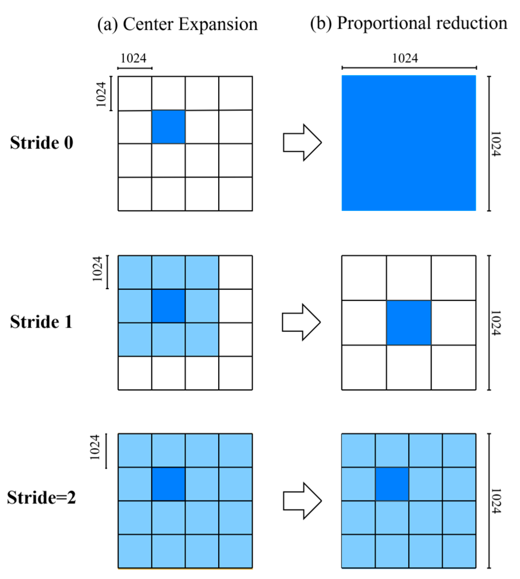
D, this study adopts a center dilation contraction method for image segmentation. The detailed procedure of the center dilation contraction method, utilized in the method of fine-grained high-resolution remote sensing image change detection involving the fusion of the SAM, is depicted in
Figure 9. Here, x and y represent the positions of the central cell, with stride indicating the dilation step based on the coordinate (x, y).
The images are uniformly divided into multiple 1024 × 1024 pixel unit grids proportionally. If a perfect proportional division is not possible, padding is applied. Each unit grid is set with a stride of one pixel. Subsequently, a sliding window technique is used to perform central dilation operations on the grids containing true values while maintaining the relative position information of the grid centers. For images that exceed the size of 1024 × 1024 pixels after dilation, they are proportionally downsized to fit the dimensions of 1024 × 1024.
- (3)
The split of the dataset
Following the commonly used 8:1:1 split ratio in the field of deep learning, the LEVIR-CD and WHU-CD datasets are divided into training, validation, and test sets. Specifically, 80% of the image data is allocated to the training set for model training and parameter tuning. This proportion ensures that the SCDM has a sufficient amount of data for learning, thereby enhancing its accuracy and robustness. The next 10% of the data is used for the validation set, which is employed for evaluating and optimizing the model during training. Finally, the remaining 10% of the image data is designated as the test set, which serves as the dataset for the final evaluation of the model’s performance.
4.2. Experiment Configuration
This experiment is implemented using the PyTorch 2.4 deep learning framework and conducted on a server equipped with four NVIDIA 3060 GPUs which were produced by NVIDIA Corporation in the USA, each with 12 Gb of memory.
The network training utilizes the Adam optimizer with a batch size of 4 on the training set. The learning rate remains constant for the first 100 epochs and is linearly decayed to 0 over the remaining 100 epochs.
4.3. Process of Experiment
For the pre-segmented LEVIR-CD dataset, a uniform size of 256 × 256 is employed as input for model training. As for the WHU-CD dataset, two variations are created using fixed-size cropping (512 × 512) and center expansion and reduction cropping (1024 × 1024) (
Figure 10). During training, data augmentation techniques such as random flipping and photometric distortions are applied. To fully exploit the model’s performance, the training epochs are set to 300, ensuring an ample number of model iterations.
- (1)
Training
The contrastive images and their label data of the training set are given.
Pairwise images and their label data are processed through the SAM-UNet module to obtain global feature maps . These are further processed through the feature difference comparison to obtain features . Subsequently, the multi-scale feature fusion module combines the global feature maps with the difference features to produce fused features. Finally, the resulting fused features are decoded through the decoder to generate the predicted change detection results Z.
A loss function called L(Z, GT) is established to measure the error between the predicted values Z and the ground truth label maps GT. Subsequently, the loss function
L is optimized using the backpropagation algorithm to iteratively optimize and train the network model parameters until the loss value converges, achieving the optimal model.
where
represents the number of categories for change detection,
denotes the value of the fine-grained contrast loss function;
is the ground truth value taking either 0 or 1, where it takes 1 if the category
matches the category of the sample, otherwise it takes 0; and
represents the probability that the predicted sample belongs to category c.
During the iterative optimization training process, the model’s training accuracy is verified in real time using a validation set, and the weights of the model with the highest accuracy are saved. Ultimately, the Mean Intersection over Union () is adopted as the evaluation metric.
- (2)
Testing
In this study, paired image and label data from the test set are fed into the trained model to predict change regions within the test set. The Intersection over Union () between the predicted change regions and the ground truth change regions is calculated, and a statistical analysis is performed based on all categories of the change regions to obtain the Mean Intersection over Union (). This metric is used to assess the prediction accuracy of change detection.
4.4. Evaluation Metrics
For the building change detection (BCD) task, we utilize the precision, recall, (Intersection over Union), score, and overall accuracy () as the model evaluation metrics. The related definitions and computation formulas are as follows:
This refers to the proportion of true positives (
) among all instances classified as positive (
+
), as follows:
- (2)
Recall
Recall refers to the proportion of true positives (
) among all instances that are truly positive (
+
). The formula is as follows:
- (3)
IoU
The Intersection over Union (
), commonly used to evaluate the performance of object detection and semantic segmentation, is a critical metric. The numerator represents the overlapping area between the predicted bounding box and the ground truth bounding box, while the denominator represents their union, which is the total area covered by both the predicted and ground truth bounding boxes. The formula is as follows:
Specifically, the concept of the Mean Intersection over Union (
) is introduced:
where
represents the set of pixels identified as the changed area by the model, while
represents the set of pixels in the changed area as per the true labels. The Mean Intersection over Union (
) typically ranges from 0 to 1, with values closer to 1 indicating better model performance, signifying that the model’s predicted segmentation is more closely aligned with the actual annotations.
- (4)
Overall Accuracy
The overall accuracy represents the proportion of all correctly predicted samples to the total number of predicted samples. It is derived according to the following formula:
- (5)
F1 score
The
score can be interpreted as the weighted average of the
and
(
), and a higher
score indicates a better robustness of the model. Its formula is as follows:
where
represents true positives, which are correctly identified changes;
represents false positives, indicating changes that are incorrectly identified;
represents false negatives, representing changes that were not identified;
represents true negatives, indicating correctly identified no-changes. The
and
, respectively, denote the accuracy and recall of change categories; the
represents the Intersection over Union for the same category;
represents overall accuracy.
4.5. Experimental Analysis
4.5.1. Comparative Experiments
The proposed SCDM is comprehensively evaluated through experiments and compared with other change detection methods, including DTCDSCN, STANet, BIT, ChangeFormer, Tiny-CD, and ChangerEx, on the LEVIR-CD and WHU-CD datasets, as shown in
Table 1 and
Table 2, respectively. It can be observed from the tables that on the LEVIR-CD dataset, the SCDM achieves the best values for both the recall (
) and Intersection over Union (
), reaching 94.62% and 84.72%, respectively. This indicates that the SCDM exhibits high sensitivity in identifying changed areas and performs excellently in terms of the overlap between the predicted and actual changed areas. Despite a slightly lower precision (
) and F1 score compared to the ChangerEx model, the SCDM still maintains a leading position in overall performance.
Furthermore, on the WHU-CD dataset, the SCDM demonstrates the best performance in terms of its score and , with values of 92.28% and 84.76%, respectively. This further confirms the stability and reliability of the SCDM across different datasets. Particularly noteworthy is the significant improvement in recall compared to the ChangeFormer model, increasing from 89.31% to 93.21%. This suggests that the SCDM is capable of detecting all changed areas more comprehensively.
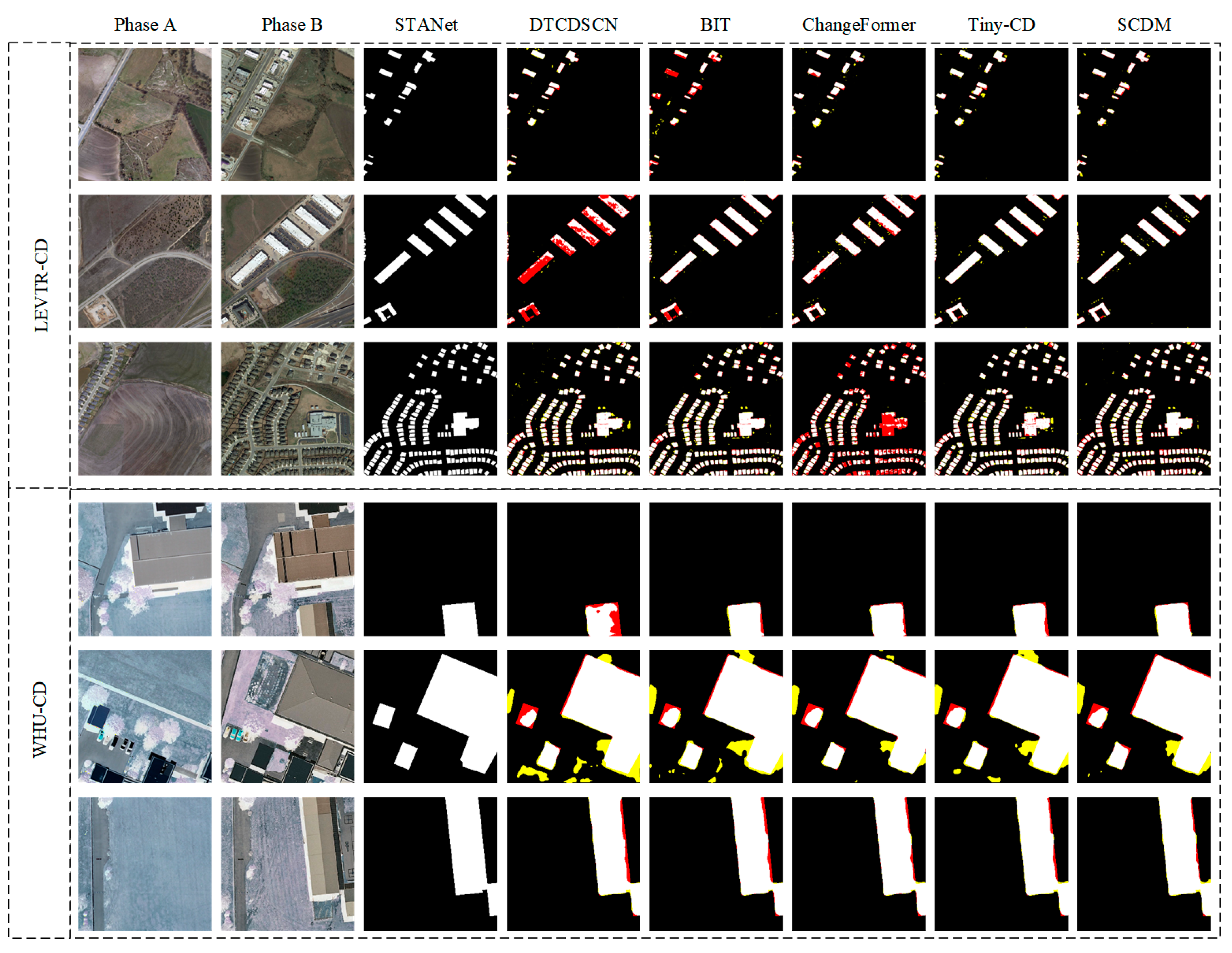
Figure 11 presents partial visual comparison results between the LEVIR-CD and WHU-CD datasets. It is evident from
Figure 11 that while STANet, DTCDSCN, BIT, ChangeFormer, and the Tiny-CD method exhibit no false detections on the LEVIR-CD dataset, they tend to miss more in the building edge regions. Conversely, the SCMD method demonstrates promising performance on the LEVIR-CD dataset. Meanwhile, STANet and DTCDSCN methods exhibit results on the WHU-CD dataset similar to those on the LEVIR-CD dataset. However, BIT, ChangeFormer, and the Tiny-CD method not only exhibit missing detections but also show multiple false detection areas on the WHU-CD dataset. In comparison to STANet, DTCDSCN, BIT, ChangeFormer, and the Tiny-CD method, the SCMD method performs better on the WHU-CD dataset, with only occasional missing detections in complex small regions.
4.5.2. Ablation Study
To compare different data-splitting methods and validate the effectiveness of the proposed SAM fusion and fine-grained loss functions, a series of ablation experiments are conducted in this study. The proposed methods are compared with state-of-the-art approaches for six BCD tasks on the WHU-CD and LEVIR-CD datasets. Specifically, traditional fixed-size splitting and expansion and reduction methods were initially applied to split the datasets. Evaluation metrics, including the
(
),
(
),
score, and Intersection over Union (
), were used to assess the impact of different data-splitting methods on model performance. The results, as shown in
Table 3 and
Table 4, indicate that the expansion and reduction method significantly improves model performance compared to the fixed-size splitting method. Specifically, under both splitting methods, the ChangeFormer model yielded the best results, followed by ChangerEx, Tiny-CD, BIT, DTCDSCN, and STANet. The use of the expansion and reduction method notably enhanced the precision of the DTCDSCN, STANet, BIT, ChangeFormer, Tiny-CD, and ChangerEx models, with respective increases in F1 scores of 0.47%, 1.19%, 0.43%, 1.88%, 1.74%, and 1.54% and respective increases in their
of 1.21%, 2.66%, 0.59%, 1.22%, 0.92%, and 0.87%.
In addition, this study explores the impact of integrating the SAM and fine-grained loss function on model performance on the WHU-CD dataset, as presented in
Table 4. From the table, it can be observed that the traditional Unet model yields the lowest accuracy, with precision (
), recall (
),
score, and Intersection over Union (
) scores of 82.85%, 85.31%, 84.06%, and 76.93%, respectively. The SCDM incorporating the center expansion and reduction method, SAM fusion, and fine-grained loss function, achieves the highest accuracy, with F1 and IoU scores improved by 4.06% and 3.07%, respectively. This outcome validates the effectiveness of the enhancement modules.
4.5.3. Generalization Validation
The LEVIR-CD and WHU-CD datasets provide relevant data but do not fully capture the diversity of real-world scenarios encountered in remote sensing. To address this limitation, this study incorporates additional dataset DTX representing varying resolutions, spectral features, and geographic contexts.
This study defines the data collection area as the DTX region, with boundaries of 5 km × 5 km covering an area of 25 km
2. The UAV altitude is set to 100 m to ensure comprehensive coverage and clear imagery of the entire area. During the UAV flight with a high-resolution camera, it uses DJI Pilot V2.5.1.15 software to plan the flight path, set waypoints, and ensure the complete coverage of the area. After data collection, it uses DJI Terra 3.0.0 to stitch the images and generate orthophotos. The DTX dataset is categorized into Phase A and Phase B. Phase A consists of images from the first UAV flight, and Phase B consists of images from the second UAV flight, as shown in
Figure 12. The DTX dataset defines a total of eight classes based on project requirements, including one background class. The classes are as follows: Woodland, Grassland, Buildings, Shed, Road, Bareland, Water, and Others.
A total of three batches of DTX data were produced: Phase 1 with 139 images, Phase 2 with 616 images, and Phase 3 with 1521 images. Comparative experiments were conducted on the provided DTX dataset, and the model performance was evaluated. The best values are indicated in bold. The relevant experimental data are presented in the
Table 5.
On this dataset, the SCDM achieved optimal values in both (R) and Intersection over Union () metrics, with scores of 88.56% and 82.23%, respectively. This indicates that the SCDM exhibits high sensitivity in identifying changed areas and performs exceptionally well in predicting the overlap between detected changes and actual changes. The model achieved an accuracy () of 84.68%. Although its () is slightly lower than that of ChangerEx and its score is marginally lower than that of Tiny-CD, the SCDM maintains a superior overall performance.
Predictions were made using the trained model, and the results are illustrated in
Figure 13, where White
(true positive) denotes correctly identified changes, Yellow
(false positive) represents incorrectly identified changes, Red
(false negative) indicates missed actual changes, and Black
(true negative) shows correctly identified non-changes.
From the comparative experimental results, it is evident that the proposed algorithm, the SCDM, demonstrates superior performance in the field of remote sensing image processing. The experimental results highlight the following advantages of the proposed algorithm: (1) it significantly enhances the contrast and clarity of remote sensing images; (2) it preserves a substantial amount of detail, avoiding the detail loss common in traditional algorithms; (3) it performs exceptionally well in complex scenes, with notable edge sharpening effects; and (4) it is applicable to various types of remote sensing image processing. These advantages ensure that our algorithm not only provides high-quality data sources for subsequent tasks, such as object detection and recognition, but also shows promising potential for practical applications.
4.5.4. Efficiency
In terms of inference speed, we conducted image prediction inference tasks on a server equipped with four NVIDIA 3060 GPUs. The input consists of remote sensing images from two different time periods with a resolution of 1024 × 1024. Using the trained model weights for inference, the output prediction images also have a resolution of 1024 × 1024. During inference, the average processing time per image is approximately 200 milliseconds. Although constrained by the current hardware conditions, the inference speed of this model is somewhat slower compared to some higher-performing models available on the market, but it meets the project’s design requirements and performs excellently in practical applications.
Compared to other classical methods, our algorithm preserves image detail information more effectively while significantly enhancing the contrast between target regions and backgrounds. Especially in complex scenes, where traditional methods often lose some detail or exhibit excessive smoothing, our algorithm sharpens target edges, making them more distinct from the background. The comparison of model parameters (Params) and computational complexity (FLOPs) is shown in the
Table 6.
The SCDM exhibits significant advantages in inference performance, particularly in balancing parameters, computational complexity, and practical deployment. First, the SCDM’s parameter count is only 3.35 M, which is several orders of magnitude lower compared to DTCDSCN’s 41.07 M, ChangeFormer’s 41.02 M, and STANet’s 16.93 M. This substantial reduction in parameter count enables the SCDM to outperform these larger models in terms of memory usage, especially in memory-constrained devices. Although Tiny-CD has a lower parameter count (0.28 M), the SCDM offers superior feature learning capability and generalization performance while maintaining lightweight characteristics, achieving a better balance in practical applications.
In terms of computational complexity, the SCDM’s FLOPs stand at just 14.29 G, significantly lower than ChangeFormer’s 230.25 G and DTCDSCN’s 52.83 G. Even when compared to relatively lightweight models like ChangerEx (23.82 G) and STANet (26.32 G), the SCDM demonstrates higher computational efficiency. This drastically reduces the hardware computational requirements during model inference, indicating that the SCDM performs exceptionally well not only on server-side deployments but also when maintaining smooth inference speeds on edge devices and in low-computation environments.
Additionally, the SCDM offers faster inference speeds and lower energy consumption, making it highly suitable for deployment in real-time application scenarios. Compared to larger models such as DTCDSCN and ChangeFormer, the SCDM achieves higher inference efficiency with minimal parameters and computational complexity, providing significant convenience for model deployment and scalability. Consequently, the SCDM holds remarkable advantages in model lightweighting, inference speed, and hardware adaptability, making it particularly well suited for resource-constrained environments.
5. Conclusions
For the problem of building change detection, this study proposes a novel solution, namely the SCDM, which integrates the center expansion and reduction method (CERM), the Segment Anything Model (SAM), UNet, and a fine-grained loss function. Furthermore, the innovative modules, including the Global Feature Extractor (GFE), feature space metric evaluation module (FM), Global and Differential Feature Fusion Module (GDF), and Global Decoder Module (GD), are introduced. The aim of this study is to enhance the accuracy of building change detection tasks by conducting ablation studies and comparative experiments to fully evaluate the performance of the model on publicly available datasets such as the WHU-CD and LEVIR-CD.
First, the CERM is introduced to address the scale differences and morphological changes inherent in building change detection. Compared to traditional fixed-size patch-based methods, the CERM can better adapt to building changes in varying scales and shapes, thereby improving the model’s robustness. Crucially, the SAM is embedded into the model to enhance its attention and feature extraction capabilities towards crucial information. The SAM learns the correlations between each pixel, enabling the model to better capture spatial information of building changes, thus enhancing detection accuracy. Lastly, to further optimize the model training process, a fine-grained loss function is designed to finely measure the differences between model outputs and ground truth labels, thereby further improving model performance. The experimental results indicate that compared to the traditional fixed-size patch-based methods, the proposed CERM in this study significantly improves the accuracy of the ChangeFormer, ChangerEx, Tiny-CD, BIT, DTCDSCN, and STANet models. Furthermore, through comparisons with six outstanding change detection methods, the proposed SCMD method in this study demonstrates superior performance on the WHU-CD and LEVIR-CD public datasets compared to the comparative models, confirming its excellent generalizability.
In terms of future prospects, further exploration of the applicability of the SCDM in more datasets and scenarios is warranted. Additionally, consideration can be given to optimizing the model structure to enhance its operational efficiency and generalization capability. Moreover, by integrating deep learning with traditional image processing techniques, further improvements in the performance and practicality of building change detection tasks can be achieved, thereby providing more reliable and efficient solutions for urban management, environmental monitoring, and related fields.


