Technical Note

Damage Scene Change Detection Based on Infrared Polarization Imaging and Fast-PCANet

1
National Key Laboratory of Scattering and Radiation, Beijing 100854, China
2
College of Information and Electrical Engineering, China Agricultural University, Beijing 100091, China
*
Author to whom correspondence should be addressed.
Remote Sens. 2024, 16(19), 3559; https://doi.org/10.3390/rs16193559
Submission received: 20 August 2024 / Revised: 22 September 2024 / Accepted: 23 September 2024 / Published: 25 September 2024

Abstract

:
Change detection based on optical image processing plays a crucial role in the field of damage assessment. Although existing damage scene change detection methods have achieved some good results, they are faced with challenges, such as low accuracy and slow speed in optical image change detection. To solve these problems, an image change detection approach that combines infrared polarization imaging with a fast principal component analysis network (Fast-PCANet) is proposed. Firstly, the acquired infrared polarization images are analyzed, and pixel image blocks are extracted and filtered to obtain the candidate change points. Then, the Fast-PCANet network framework is established, and the candidate pixel image blocks are sent to the network to detect the change pixel points. Finally, the false-detection points predicted by the Fast-PCANet are further corrected by region filling and filtering to obtain the final binary change map of the damage scene. Comparisons with typical PCANet-based change detection algorithms are made on a dataset of infrared-polarized images. The experimental results show that the proposed Fast-PCANet method improves the PCC and the Kappa coefficient of infrared polarization images over infrared intensity images by 6.77% and 13.67%, respectively. Meanwhile, the inference speed can be more than seven times faster. The results verify that the proposed approach is effective and efficient for the change detection task with infrared polarization imaging. The study can be applied to the damage assessment field and has great potential for object recognition, material classification, and polarization remote sensing.

1. Introduction

A crucial aspect of assessing damage via optical image change detection is the precise extraction of change information [1]. The accuracy of the change detection heavily relies on the quality of the extraction results. However, the current optical imaging system is vulnerable to various natural environmental factors, such as rain, snow, and smoke. This can result in the generation of noise and background interference, which may impair the accuracy and efficiency of image change detection methods. Therefore, a single mode of optical image information is inadequate for precisely analyzing the damage’s severity.
Infrared polarization imaging is a novel technology that utilizes the polarization characteristics of the target radiation light wave. Compared to traditional infrared imaging technology, it not only provides the intensity information of infrared radiation but also increases the polarization characteristics including the Stokes parameters, degree of polarization, angle of polarization, and other parameters, which can effectively improve the contrast between the objects and backgrounds to enhance the ability of object identification and classification [2,3]. It is widely applied in several applications, such as camouflage detection [4], material classification [5], and atmosphere remote sensing [6]. In the field of damage assessment, infrared polarization imaging has been primarily driven by the need to enable change detection of man-made objects. Zhao [7] proposed a change detection method based on polarization image fusion in the visible band through the mapping relationship between polarization parameters and spectral parameters. Qong [8] developed a change detection algorithm based on the polarimetric basis transformation along with the polarization signatures in polarimetric SAR images, which attempts to maximize the resemblance between the scattering geometries in multidate images for a specific target. Previous studies of change detection have mainly focused on visible and SAR polarization images. They also suggest that infrared polarization imaging technology has potential advantages in the field of damage scene change detection.
To the best of our knowledge, few works have studied infrared polarization imaging for damage scene change detection. In the literature, many change detection approaches have been proposed in the field of remote sensing, mainly for optical images [9,10,11,12]. The detection methods are used to identify changes from two images captured in the same geographic area but at different times. Both classic and deep learning-based approaches have been developed. Traditional methods usually obtain the difference image (DI) directly and further recognition of the changed pixels and un-changed pixels from the DI through discrepancy analysis, such as change vector analysis (CVA) [13], slow feature analysis (SFA) [14], iteratively reweighted multivariate alteration detection (MAD) [15], and PCA-Kmeans [16]. Deep learning-based methods generally focus on image feature extraction and improve the change detection performance by discerning the potential changes in the robust feature space. Ma [17,18] developed a multi-criteria decision network (MCDNet) to achieve higher-quality sample labeling and more accurate detection results and a coarse-to-fine detection network through multiscale super-resolution enhancement and multilevel attention fusion for infrared images. Saha [19] proposed a new unsupervised context-sensitive framework, depth variation vector analysis (DCVA), for multi-temporal high-resolution image change detection. Zhang [20] utilized a deep belief network (DBN) to extract abstract, invariant features directly from the original image. They then mapped the changed features of the dual-temporal image to the 2D polar domain and employed an unsupervised clustering algorithm to generate change detection results. YunLin [21] trained a model using two symmetric convolutional neural networks to learn feature representations from dual temporal phase images. They then applied these features to a softmax classifier to obtain the final change results. Seda et al. [22] utilized a supervised (E-ReCNN) and semi-supervised (SVM-STV) approach to study binary and multi-class change within mining ponds in the Madre de Dios region obtained Sentinel-2 imagery. Feng [23] proposed a PCANet-based change detection method for synthetic aperture radar images. They used the PCANet proposed by Chan [24] to extract the change and invariant features. Among these methods, the PCANet-based method has a simple network structure and can produce good results with a small number of training samples, which shows great potential for damage scene change detection tasks. However, the original PCANet is generally too slow to encode the image features, which presents a significant challenge to meeting real-time demands. In addition, the original PCANet does not take the multiple hierarchical deep features, making the PCANet-based change detection method impractical to effectively leverage multiple scale features to achieve optimal detection results. Furthermore, the infrared polarimetric information is a very important imaging characteristic that may further boost the change detection performance. However, it is left unexplored in the literature to the best of our knowledge.
In this paper, we propose an effective scene change detection method based on infrared polarization information and Fast-PCANet. It takes into account the specific characteristics of infrared polarization imaging and addresses the practical requirements of damaged scenes. The method first performs Stokes analysis on the infrared polarization image to obtain different infrared polarization parameter images. Second, it extracts and filters the pixel image blocks, filtering out most of the unchanged pixels and pixels with small changes in the time-phase difference image and obtaining the candidate change point image blocks. Then, it builds the Fast-PCANet framework and feeds the candidate change point image blocks to predict the change pixel points in the network. Finally, the false-detection points detected in the Fast-PCANet module are further corrected by region filling and filtering. The proposed approach can improve the performance in terms of the accuracy and speed for the damage scene change detection.

2. The Theoretical Algorithm

The polarization state of infrared light reflected or emitted from an object’s surface can be described using the Stokes vector [25]: S = I , Q , U , V T . Physically, I refers to the total radiance intensity, Q indicates the difference between parallel and perpendicular polarization, U models the degree of the diagonal polarizing component in the π/4 direction, and V represents the circular polarizing component. Since the circular polarizing value of natural objects is very small in infrared bands, V is usually neglected. To measure the polarization state of the light wave, the easiest way is to change the angle between the transmission axis of the polarizer and the selected reference coordinate axis and select four specific angles (usually 0, π/4, π/2, and 3π/4), respectively, so that the intensity of the light in four different polarization directions is obtained from the output of the infrared detector and then solve for the three Stokes vector parameters of the light wave. The expressions for I, Q, and U are written as
I = I 0 + I π 2 Q = I 0 I π 2 U = I π 4 + I 3 π 4
where I(θ) (θ = 0, π/4, π/2, 3π/4) are the light intensities obtained by the rotary polarizer orientations at 0, π/4, π/2, and 3π/4. The expression of the degree of linear polarization (DoLP) and the angle of polarization (AoP) is written as follows:
D o L P = Q 2 + U 2 I , A o P = 1 2 arctan U Q
In infrared polarization image detection, the infrared polarization characteristics of the scene can be characterized by infrared polarization parametric images, and each parametric image reflects the intrinsic polarization information of the object from different perspectives, thus providing the basis for change detection of the damage scene.

3. The Scene Change Detection Algorithm Based on Fast-PCANet

In order to improve the accuracy of the damage scene change detection, a scene change detection algorithm based on Fast-PCANet is proposed. The framework of the algorithm is shown in Figure 1. It consists of three major steps: the pixel image block extraction and screening module filters out most of the unchanged and slightly changed pixel points in the time-phase difference image to obtain the candidate change point image blocks; the candidate change point image blocks are sent to the Fast-PCANet module to predict the changed pixel points; and the false-detected points detected in the Fast-PCANet module are further corrected by the region filling and filtering module to produce the final change detection results.

3.1. Pixel Image Block Extraction and Filtering Module

As Fast-PCANet recognizes and classifies the input at the image patch level, we first extract small image patches around each pixel, i.e., building pixel image blocks. Then, the image block corresponding to each pixel point is taken as the input of the extraction and filtering module. Furthermore, to enhance the detection efficiency of the Fast-PCANet model, the pixels in the difference image will undergo coarse screening to eliminate most of the invariant points. The whole process is outlined as follows:
  • The difference image before and after the scene change is obtained by differentiating the pre-change image and post-change image. Concretely, the difference image is a summarization of three difference images, i.e., the absolute difference between the pre-change intensity image I and the post-change intensity image I, the absolute difference between the pre-change image DoLP and the post-change image DoLP, and the absolute difference between the pre-change image AoP and the post-change image AoP.
  • The neighborhood of each pixel point in the difference image is constructed as a block of k1 × k1 size.
  • Coarse screening removes most of the invariant points from the difference image. The difference grayscale image A d i f f is binarized using an estimated change threshold. It is calculated as follows:
    A d i f f x , y = 1 , T d i f f A d i f f x , y 0 , T d i f f < A d i f f x , y
    where (x, y) are the pixel point coordinates and T d i f f is the change threshold.
Since difference images have different data distributions for invariant and change points, the optimal change threshold is obtained by solving an optimal problem by maximizing the interclass variance. Given a change threshold of T, the number of change points is Nc, the set of change points is Vc, the number of invariant points is Nuc, the set of invariant points is Vuc, V = V c V u c , the index of the element in V is V = [v1,v2,...,vNpixel], and the total number of pixels is N p i x e l = N u c + N c . The interclass variance δ between the change pixels and the invariant pixels can be calculated using the following formula:
δ ( T i ) = N c N p i x e l i = 1 N p i x e l ( v i v ¯ c ) 2 + N uc N p i x e l i = 1 N p i x e l ( v i v ¯ u c ) 2 , i = 1 , 2 , , N s a m p l e
where v ¯ c and v ¯ u c are the mean values of V c and V uc , respectively. The pixel points are arranged in ascending order of the total change value, and N s a m p l e points are sampled in equal proportions. The threshold for solving the interclass variance is determined by traversing the total change value of the sampled pixel points. Finally, the threshold with the largest interclass variance is selected.
T d i f f = arg max ( δ ( T i ) ) , i = 1 , 2 , , N s a m p l e
4.
Points with a value A d i f f of 1 are considered candidate change points, and the corresponding image block is taken as the output of this module.

3.2. Fast-PCANet Module

The Fast-PCANet is built upon the original PCANet. The PCANet is a deep learning network model that is based on convolutional neural networks (CNN) and offers a simplified structure. It can be easily trained even with a small number of samples to produce good results. However, the output layer of the PCANet takes a long time to encode the final features, which makes it a challenge to meet real-time demands. This paper proposes Fast-PCANet, an efficient and effective network customized for change detection. It improves the original PCANet network in terms of detection accuracy and inference speed. Concretely, the proposed network framework mainly comprises two PCA convolutional layers, an output layer, and a classification layer, which are illustrated in Figure 2.
PCA convolutional layer: The input is the candidate change point image blocks obtained from the pixel image block extraction and screening module. Assuming a set of N original input images I i i = 1 N , and the dimensions of each image are m × n. In the PCA convolutional layer 1, we use L1 PCA convolutional filters W l 1 of size k1 × k2 to perform the convolutional operation on the input data, resulting in N × L1 feature maps of size k1 × k2. The convolutional output for each image after the PCA convolutional layer 1 is:
I i l = I i W l 1 , l = 1 , 2 , , L 1
The input of PCA convolutional layer 2 is the feature map I i l derived from PCA convolutional layer 1. A convolutional operation is performed on the feature maps of PCA convolutional layer 1 using L2 PCA convolutional filters W l 2 of size k1 × k2 to obtain N × L1 × L2 feature maps of size k1 × k2. The outputs of each convolutional layer are then composed as:
O i l = I i W l 2 l = 1 L 2 , l = 1 , 2 , , L 1
Output layer: Unlike the original PCANet performing binarization and hash coding in the output layer, Fast-PCANet adopts layer normalization [26]. Concretely, it normalizes the output feature maps of PCA convolutional layer 1 and PCA convolutional layer 2 independently and then merges the normalized outputs in dimension. Since Fast-PCANet does not involve time-consuming operations, i.e., binarization and hash coding, but only reduces the dimension to one-dimensional vectors in the output layer, it greatly reduces the computational consumption. The layer normalization for each output convolutional layer is calculated as follows:
O ˜ i l = O i l E O i l V a r O i l
where E O i l and V a r O i l are the mean and variance of outputs of convolutional layer l .
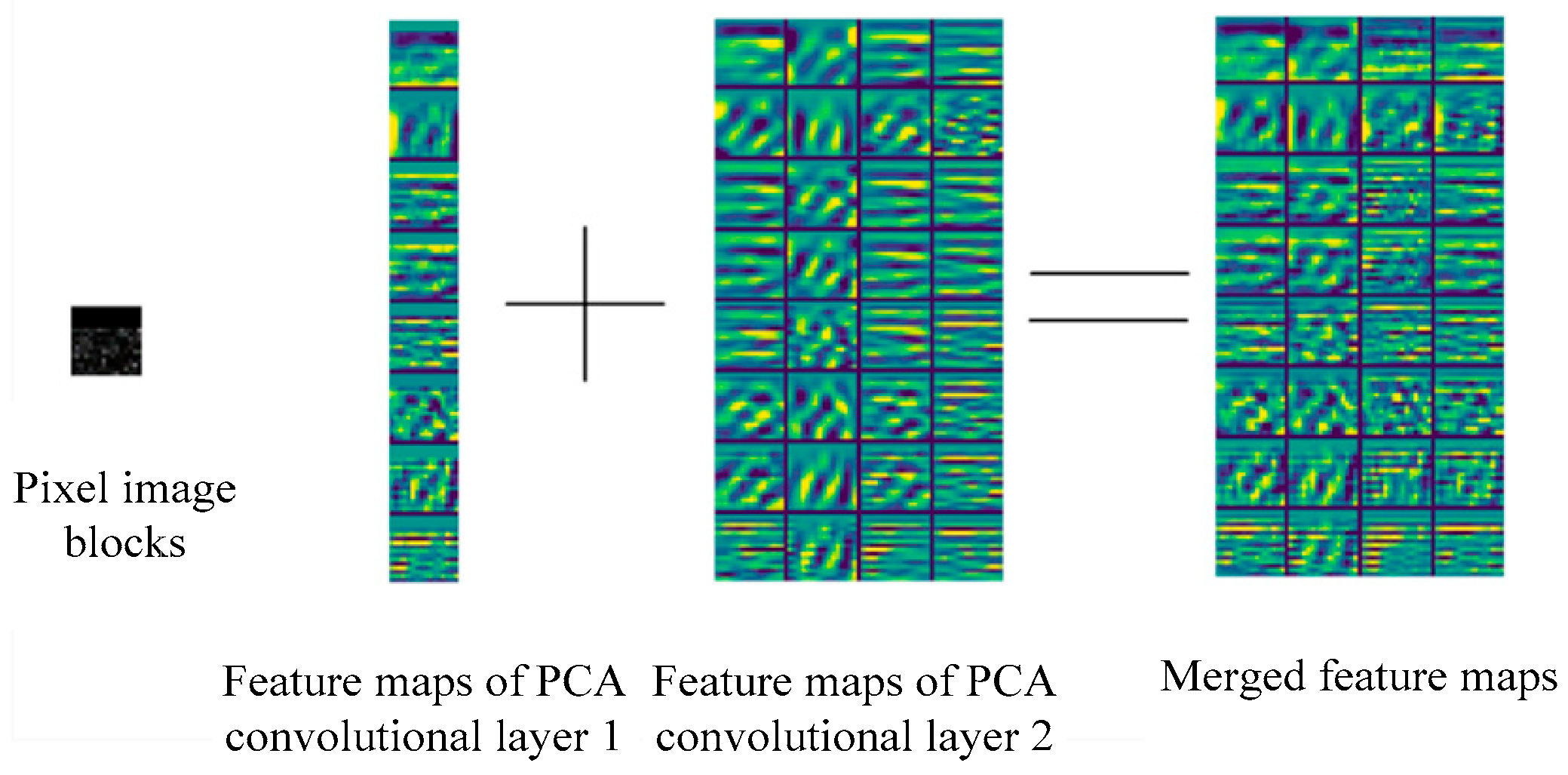
In addition, to prevent the loss of shallow information in the output feature vector, the feature map of PCA convolutional layer 1 is merged with that of PCA convolutional layer 2. Concretely, the PCA feature maps of layer 1 and layer 2 are concatenated together in their feature dimension. On the one hand, the feature maps of each PCA layer have different feature dimensions; thus, they cannot be simply summarized together. On the other hand, the concatenated feature map may contain much richer information, thus enabling a more effective characterization of the changes in pixel points. Finally, the merged feature map’s dimension is the sum of the feature dimensions of layer 1 and layer 2. The diagram of the output layer of Fast-PCANet is illustrated in Figure 3.
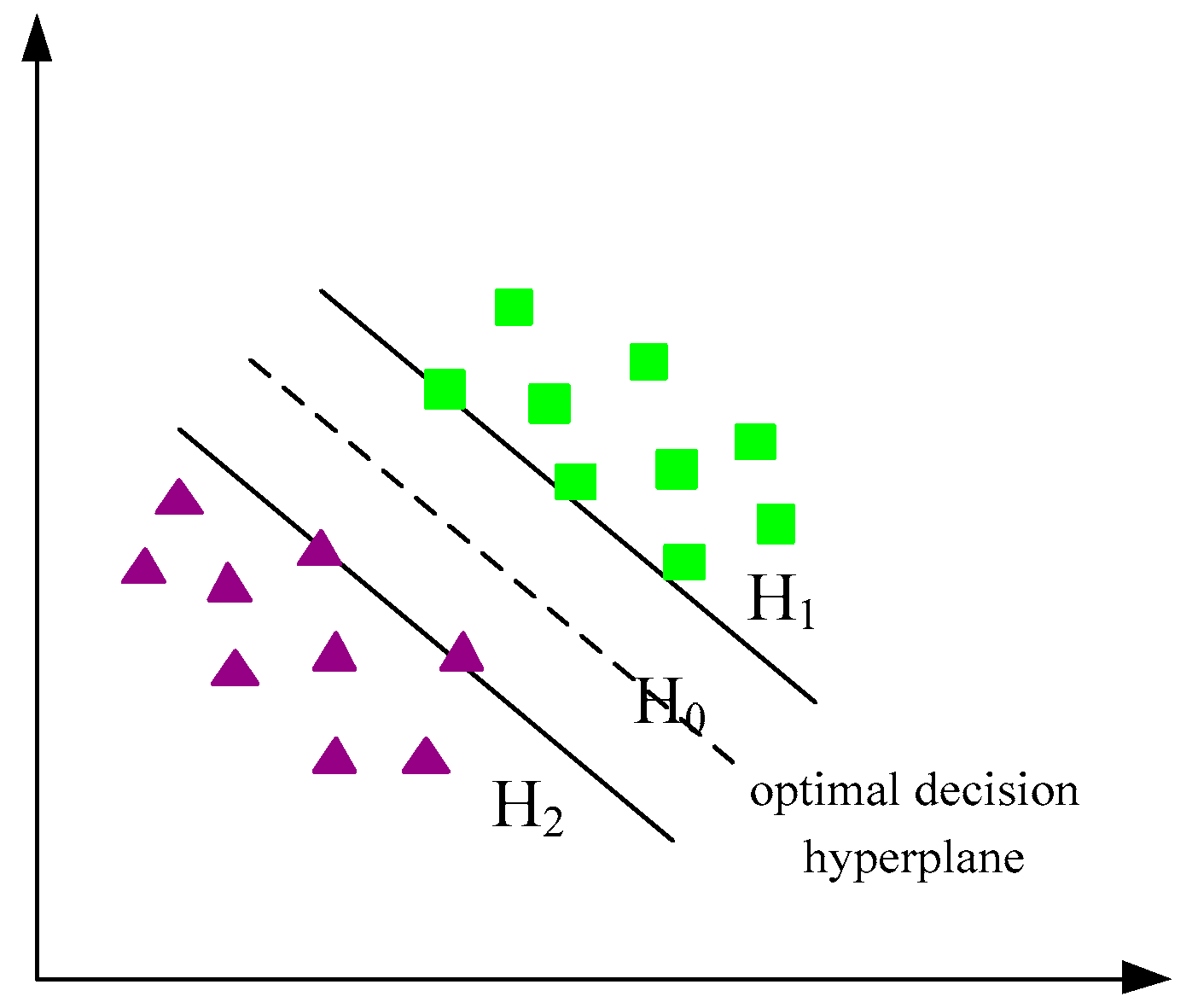
Classification layer: The output feature maps should finally be processed and detected to produce a binary change map for change detection. In this paper, we have chosen to use the linear support vector machine (SVM) [27] classifier to binary classify the features of the candidate images. The main idea is to construct the optimal decision hyperplane for the two-dimensional linearly divisible case in the original space. This maximizes the distance between the two types of samples located on both sides of the plane that are closest to the plane. The optimal decision hyperplane is then used as the classification interface to achieve the classification function. Figure 4 illustrates the schematic of the optimal hyperplane in the two-dimensional linearly divisible scenario. The green square and purple triangle points represent two different categories of samples. The dotted line H0 in the middle is the optimal decision hyperplane, while the two solid lines H1 and H2 are the two parallel surfaces closest to the optimal hyperplane. The distance between these two parallel surfaces is the classification interval of the two categories. In each of these parallel surfaces, samples from different classes are referred to as support vectors. The classification mechanism is illustrated in Figure 4.

3.3. Region Filling and Filtering Module

To further filter out the false-detection points in the binary change map, we design a region filling and filtering module for post-processing. The false detection points generally lead to breaks in the target change region or sporadic noise outside the change region. Therefore, it is necessary to fill the change region and remove the noise to correct the false detection points. The post-processing operation includes two steps: region filling and noise removal.
Region filling. We use the closed operation method, which is a method of morphological image processing. It is generally used to fill small voids within an object, connect neighboring objects, and smooth its boundary without significantly changing its area. The closed operation is defined as A B = A B B where A is the original image and B is the structural element. The symbols , , and represent the expansion operation, the corrosion operation, and the closed operation, respectively.
Noise removal. We use median filtering to remove noise from the changed area. This involves sorting the pixel values of the current pixel point and its surrounding neighboring region pixel points in the detected image and using the pixel value ranked in the middle position as the value of the current pixel point to filter out the noise.

3.4. Algorithmic Implementation

The training samples for the change detection model comprise pre- and post-change images as well as labeled maps. The change detection process involves the labeling of the target change region, with the remainder of the region designated as unchanged. The image blocks corresponding to the change points and invariant points are transformed into positive and negative samples. The non-target change points, such as shadow changes, light changes, and alignment errors, are categorized as invariant points. In general, the number of change points in change detection is considerably smaller than that of invariant points. The discrepancy between the positive and negative samples is significant, reducing the likelihood of model overfitting and facilitating the detection of changes. Furthermore, the data distribution of invariant points is not uniform, with a disproportionately low prevalence of high-value invariant point data. The majority of invariant points are concentrated in the low-value region, while a small number are located in the high-value region. These high-value invariant points are frequently pseudo-change points, which must be incorporated into the negative samples to ensure that each value region of the invariant points is represented, thereby enhancing the generalization capacity of the negative samples. Consequently, in the case of change points with insufficient data, these will be incorporated as positive samples, whereas in the case of invariant points, a selective screening process will be employed in order to achieve a balanced ratio of positive and negative samples. The procedure for the generation of positive and negative samples for each training image is as follows:
  • It is necessary to extract the image block of each pixel point of the differential image, both before and after the change.
  • The differential image pixel points are to be divided into change points and unchanged points based on the labeling map. Each of these is then to be sorted according to the numerical size, from largest to smallest.
  • It is assumed that the error rate associated with manual labeling is 5%. Consequently, the number of erroneous points to be removed is 5% of the total number of change points. The change points are eliminated in descending order of magnitude to obtain the change point set V c , while the invariant points are eliminated in ascending order of magnitude to obtain the invariant point set V u c .
  • The image blocks corresponding to all points in the change point set should be designated as positive samples for model training.
  • The sorted pixel points in the invariant point set are sampled using the second-order equivariant series, thereby enabling the capture of invariant points within each value region. The general formula for the second-order isotropic series is as follows:
    a n = n a 1 + n ( n 1 ) d 2 , n = 1 , 2 , , N s a m p l e 2
    where N s a m p l e 2 is the number of invariant points to be sampled, a n is the pixel index of the nth sampling point, and assuming a 1 = 1 , a N s a m p l e 2 = l e n ( V u c ) , then the isometry d is
    d = 2 ( a N sample 2 N s a m p l e 2 a 1 ) N s a m p l e 2 ( N s a m p l e 2 1 )
  • Following step 5, the image block corresponding to the sampling point is generated as a negative sample for model training, and the positive and negative samples are produced.
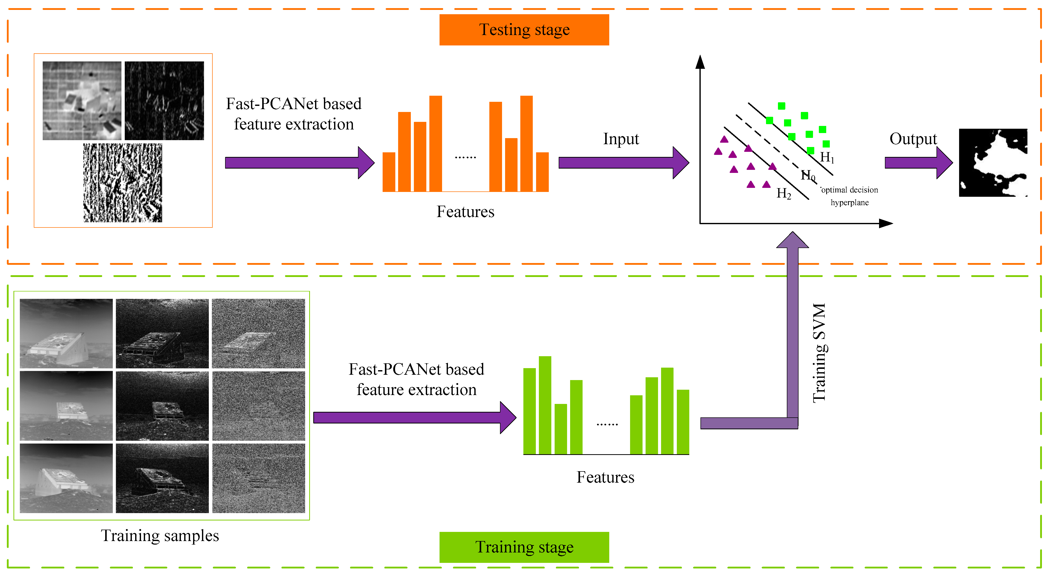
In the model training stage, the Fast-PCANet model is trained in a manner analogous to that of the PCANet model. The positive and negative sample image blocks are input, and the image blocks are cascaded according to the size of the sliding window in order to construct the feature vectors of each image block. The optimal standard orthogonal matrices of PCA convolutional layer 1 and PCA convolutional layer 2 are identified as the PCA convolutional filter parameters of the layers, respectively. Subsequently, the SVM is trained using the Fast-PCANet model output feature vectors as the training samples of the SVM. Subsequently, the PCA filter parameters of PCA convolutional layer 1 and PCA convolutional layer 2, along with the SVM model parameters, are stored for future reference. In the model testing stage, the unlabeled image blocks are fed into the Fast-PCANet model, the trained PCA filter parameters are called upon to perform the convolution directly, and then the feature vectors produced by the Fast-PCANet model are fed into the SVM in order to predict the change results, as shown in Figure 5.

4. Experiment and Analysis

4.1. Datasets

At present, there is no open-source dataset for infrared polarization images of damage scenes. Therefore, the dataset used in the experiments of this paper was derived from the actual acquisition of infrared polarization image data of the change scene. We used a division-of-focal-plane type infrared polarization imaging device [28] to carry out pre-change and post-change infrared polarization imaging acquisition experiments on a typical man-made target. Simultaneously, we obtained the target’s four ways of polarization information at angles of 0, π/4, π/2, and 3π/4. We then conducted Stokes parametric image analysis to obtain three types of infrared polarization characteristics, namely I, DoLP, and AoP. This allowed us to construct an infrared polarization characteristics dataset. The MESR-SURF [29] image alignment algorithm was used to align the target area due to slight differences in the positions captured by the infrared polarization imaging device before and after the change. The dataset comprises 859 pre-change and post-change infrared polarization images, with a waveband of 8~14 μm and an image size of 640 × 480. It includes various target images of the changing scene at different angles and is divided into a training set and a test set in a 9:1 ratio. Figure 6 displays the changed I (denotes the infrared intensity characteristics), DoLP, and AoP images of the real damage scene at different cases.

4.2. Evaluation Index

This paper evaluates the accuracy and real-time performance of the proposed algorithm for target detection in changing scenes from different aspects. The evaluation indexes selected are the percentage correctly classified (PCC), the Kappa coefficient, and the detection speed (seconds). The expressions for the correct detection rate PCC and Kappa coefficient are provided below.
P C C = 1 F P + F N N
K a p p a = P C C P R E 1 P R E
P R E = ( T P + F P ) ( T P + F N ) + ( F N + T N ) ( T N + E P ) N 2
where the total number of pixels in the image is represented by N. False positive (FP) refers to the number of actual unchanged pixel points that are detected as changed pixel points, while false negative (FN) refers to the number of actual changed pixel points that are detected as unchanged pixel points. The number of correctly detected changed pixel points is denoted by true positive (TP), while true negative (TN) denotes the number of correctly detected unchanged pixel points. The detection effect is better when the PCC is larger. The detection performance is better when the Kappa coefficient is larger.

4.3. Architecture

In all the experiments, we use the same architecture as our proposed Fast-PCANet. Concretely, it consists of two PCA convolutions as the original PCANet [26]. The convolutional filters are 2 and 4, respectively, and the kernel size of each filter is 3 × 3.

4.4. Results

4.4.1. Overall Performance

The overall evaluation results of the proposed change detection approach on the test dataset are shown in Table 1. Our proposed approach, i.e., Fast-PCANet combined with intensity polarization features, performs better than other methods and it improves the PCC and the Kappa coefficient of infrared polarization images over infrared intensity images by nearly 6.77% and 13.67%, respectively. On the one hand, whenever combined with different kinds of feature types, Fast-PCANet always obtains a higher PCC and Kappa against the PCANet method, which implies that the proposed feature extraction mechanism, i.e., layer normalization and multi-layer merging instead of binarization and hash coding of the output of PCANet, is, in essence, more plausible than the original PCANet for the change detection task. On the other hand, the polarization feature contributes to the change detection task and boosts the detection performance. When polarization features are adopted, the PCC and Kappa of PCANet and Fast-PCANet are infrared intensity increased, respectively, since polarization characteristics can effectively improve the contrast between the objects and backgrounds, thus enhancing the ability of change identification.

4.4.2. Case Studies

To further verify the proposed Fast-PCANet approach and acquire deeper insight into the change detection method under an infrared polarization imaging scene, we analyzed several damage cases, both quantitatively and qualitatively.
The qualitative results are shown in Figure 7. The first row in Figure 7 is the post-change target area and the second row is the ground truth binary change map. The change detection results with different methods are visualized from the third to the last row. We can see that PCANet with only an intensity feature suffers from many false positive (red) and false negative (green) predictions. When enhanced with the polarization feature, the false negative points are greatly reduced. At the same time, the false positive points are also decreased. The same phenomenon happens when the proposed Fast-PCANet approach is used. This verifies the effectiveness of the polarization feature for damage scene change detection, and infrared polarization imaging may show great potential for change detection. In addition, in contrast to PCANet, our Fast-PCANet generally produces convincing change results with much fewer false detection areas against the ground truth change maps.
Table 2 qualitatively shows the detection results of each method for each damage case. It shows that the detection methods that combined intensity and polarization features have a higher performance index than that only with intensity features, and the proposed Fast-PCANet consistently outperforms the original PCANet-based methods for all cases and under all feature type configurations. The results are coherent with the conclusions presented in Section 4.4.1.

4.4.3. Speed Analysis

The inference speeds of different change detection approaches are shown in Table 3. The inference time (seconds per image) is average on the test dataset and the program is running on a computer workstation with an Intel Core i7-8700k CPU and 32 GB Memory. Compared with PCANet, our Fast-PCANet has a much faster inference speed. It further verifies that the proposed layer normalization and multi-layer merging strategy is much more efficient than that of the binarization and hash coding in the original PCANet.

5. Conclusions

To solve the problem of low change detection accuracy of traditional optical images in damage scenes, this paper proposed a change detection method that combines the Fast-PCANet network with infrared polarized images. It improves the PCANet both in detection accuracy and speed by utilizing layer normalization and multi-layer feature fusing. In addition, to the best of our knowledge, we are the first to explore polarization information for damage scene change detection. The experimental results demonstrate that the proposed approach can boost the performance index of PCC and Kappa greatly with Fast-PCANet specifically enhanced by the polarization information. The results show the effectiveness of the polarization feature for damage scene change detection, and this may also possess great potential for other change detection tasks, which we will investigate in the future.

Author Contributions

Methodology, M.Y.; algorithm, J.Y.; validation, H.M. and C.Z.; writing—review and editing, M.Y.; writing—review and editing, J.Y. All authors have read and agreed to the published version of the manuscript.

Funding

The research received no external funding.

Data Availability Statement

The original contributions are presented in this article. Future inquiries can be directed to the corresponding author.

Conflicts of Interest

The authors declare no conflicts of interest.

References

  1. Sun, C. Research on the Application of Optical Image Processing Methods in Battlefield Exercise Damage Assessment. Master’s Thesis, Xi’an Technological University, Xi’an, China, 2023. [Google Scholar]
  2. Tyo, J.; Goldstein, D.; Chenault, D.; Shaw, J. Review of passive imaging polarimetry for remote sensing applications. Appl. Opt. 2006, 45, 5453–5469. [Google Scholar] [CrossRef] [PubMed]
  3. Felton, M.; Gurton, K.; Pezzaniti, J.; Chenault, D.; Roth, L. Comparison of the inversion periods for MidIR and LWIR polarimetric and conventional thermal imagery. Proc. SPIE 2010, 7672, 76720R. [Google Scholar]
  4. Gong, L.; Yu, J.; Yang, Z.; Li, Y.; Yang, L.; Yu, Y.; Wu, Z.; Wang, L. Infrared polarization model optimization and radiation characteristics of camouflage coatings. Infrared Phys. Technol. 2024, 137, 105086. [Google Scholar] [CrossRef]
  5. Sawyer, M.A.; Hyde, M.W. Material characterization using passive multispectral polarimetric imagery. Proc. SPIE 2013, 8873, 88730Y. [Google Scholar]
  6. Qie, L.; Li, Z.; Sun, X.; Sun, B.; Li, D.; Liu, Z.; Huang, W.; Wang, H.; Chen, X.; Hou, W.; et al. Improving remote sensing of aerosol optical depth over land by polarimetric measurements at 1640 nm: Airborne test in north China. Remote Sens. 2015, 7, 6240–6252. [Google Scholar] [CrossRef]
  7. Zhao, Y.; Zhang, L.; Zhang, D.; Pan, Q. Object separation by polarimetric and spectral imagery fusion. Comput. Vis. Image Underst. 2009, 113, 855–866. [Google Scholar] [CrossRef]
  8. Qong, M. Polarization state conformation and its application to change detection in polarimetric SAR data. IEEE Geosci. Remote Sens. Lett. 2004, 1, 304–308. [Google Scholar] [CrossRef]
  9. Chen, H.; Qi, Z.; Shi, Z. Remote sensing image change detection with transformers. IEEE Trans. Geosci. Remote 2022, 60, 1–14. [Google Scholar] [CrossRef]
  10. Bai, T.; Wang, L.; Yin, D.; Sun, K.; Chen, Y.; Li, W.; Li, D. Deep learning for change detection in remote sensing: A review. Geo-Spat. Inf. Sci. 2023, 26, 262–288. [Google Scholar] [CrossRef]
  11. Afaq, Y.; Manocha, A. Analysis on change detection techniques for remote sensing applications: A review. Ecol. Inform. 2021, 63, 101310. [Google Scholar] [CrossRef]
  12. Asokan, A.; Anitha, J. Change detection techniques for remote sensing applications: A survey. Earth Sci. Inform. 2019, 12, 143–160. [Google Scholar] [CrossRef]
  13. Bovolo, F.; Bruzzone, L. A theoretical framework for unsupervised change detection based on change vector analysis in the polar domain. IEEE Trans. Geosci. Remote 2006, 45, 218–236. [Google Scholar] [CrossRef]
  14. Nielsen, A. The regularized iteratively reweighted MAD method for change detection in multi- and hyperspectral data. IEEE Trans. Image Process 2007, 16, 463–478. [Google Scholar] [CrossRef]
  15. Wu, C.; Du, B.; Zhang, L. Slow feature analysis for change detection in multispectral imagery. IEEE Trans. Geosci. Remote 2014, 52, 2858–2874. [Google Scholar] [CrossRef]
  16. Celik, T. Unsupervised change detection in satellite images using principal component analysis and k-means clustering. IEEE Geosci. Remote Sens. Lett. 2009, 6, 772–776. [Google Scholar] [CrossRef]
  17. Ma, T.; Wang, H.; Liang, J.; Peng, J.; Ma, Q.; Kai, Z. MSMA-Net: An infrared small target detection network by multi-scale super-resolution enhancement and multi-level attention fusion. IEEE Trans. Geosci. Remote 2024, 62, 5602620. [Google Scholar]
  18. Ma, T.; Ma, Q.; Yang, Z.; Liang, J.; Fu, J.; Dou, Y.; Ku, Y. Usman Ahmad, Liangqiong Qu, MCDNet: An infrared small target detection network using multi-criteria decision and adaptive labeling strategy. IEEE Trans. Geosci. Remote 2024, 62, 5613414. [Google Scholar]
  19. Saha, S.; Bovolo, F.; Bruzzone, L. Unsupervised deep change vector analysis for multiple-change detection in VHR images. IEEE Trans. Geosci. Remote 2019, 57, 3677–3693. [Google Scholar] [CrossRef]
  20. Zhang, H.; Gong, M.; Zhang, P.; Su, L.; Shi, J. Feature-level change detection using deep representation and feature change analysis for multispectral imagery. IEEE Geosci. Remote Sens. Lett. 2016, 13, 1666–1670. [Google Scholar] [CrossRef]
  21. Lin, Y.; Li, S.; Fang, L.; Ghamisi, P. Multispectral change detection with bilinear convolutional neural networks. IEEE Geosci. Remote Sens. Lett. 2020, 17, 1757–1761. [Google Scholar] [CrossRef]
  22. Camalan, S.; Cui, K.; Pauca, V.P.; Alqahtani, S.; Silman, M.; Chan, R.; Plemmons, R.J.; Dethier, E.N.; Fernandez, L.E.; Lutz, D.A. Change detection of Amazonian alluvial gold mining using deep learning and Sentinel-2 imagery. Remote Sens. 2022, 14, 1746. [Google Scholar] [CrossRef]
  23. Gao, F.; Dong, J.; Li, B.; Xu, Q. Automatic change detection in synthetic aperture radar images based on PCANet. IEEE Geosci. Remote Sens. Lett. 2016, 13, 1792–1796. [Google Scholar] [CrossRef]
  24. Chan, T.; Jia, K.; Gao, S.; Lu, J.; Zeng, Z.; Ma, Y. PCANet: A simple deep learning baseline for image classification. IEEE Trans. Image Process 2015, 24, 5017–5032. [Google Scholar] [CrossRef] [PubMed]
  25. Stokes, G. On the comparison and resolution of streams of polarized light from different sources. Trans. Camb. Philos. Soc. 1852, 9, 399–416. [Google Scholar]
  26. Xu, J.; Sun, X.; Zhang, Z.; Zhao, G.; Lin, J. Understanding and improving layer normalization. Adv. Neural Inf. Process. Syst. 2019, 32, 2–19. [Google Scholar]
  27. Hearst, M.; Dumais, S.; Osuna, E.; Platt, J.; Scholkopf, B. Support vector machines. IEEE Intell. Syst. 1998, 13, 18–28. [Google Scholar] [CrossRef]
  28. Yang, M.; Mao, H.; Xu, W.; Feng, B.; Zhai, W. DoFP polarimetric imagery in infrared detection blindness rejection. Proc. SPIE 2022, 12166, 121667W-1-10. [Google Scholar]
  29. Tao, L.; Jing, X.; Sun, S.; Huang, H.; Chen, N.; Lu, Y. Combining SURF with MSER for image matching. In Proceedings of the 2013 IEEE International Conference on Granular Computing (GrC), Beijing, China, 13–15 December 2013; pp. 286–290. [Google Scholar]
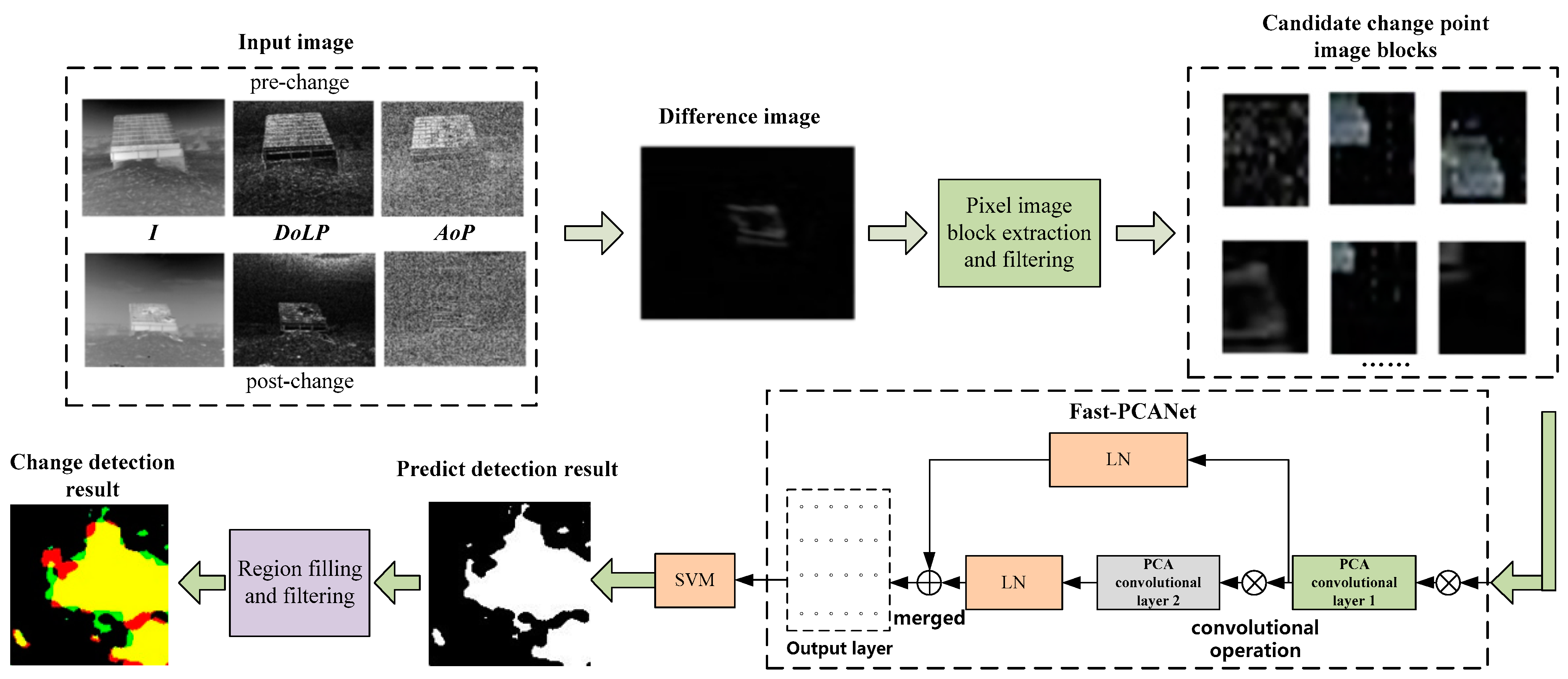
Figure 1. Algorithmic framework for damage scene change detection based on Fast-PCANet.
Remotesensing 16 03559 g001
Figure 2. Framework of the proposed Fast-PCANet for scene change detection.
Remotesensing 16 03559 g002
Figure 3. Simplified diagram of Fast-PCANet network output layer.
Remotesensing 16 03559 g003
Figure 4. The schematic diagram of the optimal hyperplane.
Remotesensing 16 03559 g004
Figure 5. The scene change detection process based on the Fast-PCANet with SVM.
Remotesensing 16 03559 g005
Figure 6. Infrared polarization images of the scene after changes at selected case. (a) infrared intensity image; (b) DoLP image; (c) AoP image.
Remotesensing 16 03559 g006
Figure 7. The change detection results of the target (damage) area, where yellow represents the true positive area, red is the false positive, and green is the false negative.
Remotesensing 16 03559 g007
Table 1. Evaluation indexes of different change detection methods on the test dataset.
MethodFeature TypeEvaluation Indexes
PCCKappa
PCANetInfrared intensity0.84120.6665
Intensity + polarization0.86320.7105
Fast-PCANetInfrared intensity0.88680.7579
Intensity + polarization0.90890.8032
Table 2. The qualitative results for the target (damage) area with different change detection methods.
MethodFeature TypeCase 1Case 2Case 3
PCCKappaPCCKappaPCCKappa
PCANetInfrared intensity0.86880.72970.80260.59370.83540.6468
Intensity + polarization0.89750.78760.83580.65580.88610.7531
Fast-PCANetInfrared intensity0.87550.743800.88000.74540.84000.6581
Intensity + polarization0.91590.82740.90270.79100.89240.7683
Table 3. The inference speeds of different change detection approaches.
MethodFeature TypeTime Cost (s)
PCANetInfrared intensity10.5515
Intensity + polarization10.4929
Fast-PCANetInfrared intensity1.4460
Intensity + polarization1.4550
Disclaimer/Publisher’s Note: The statements, opinions and data contained in all publications are solely those of the individual author(s) and contributor(s) and not of MDPI and/or the editor(s). MDPI and/or the editor(s) disclaim responsibility for any injury to people or property resulting from any ideas, methods, instructions or products referred to in the content.