Article

Regional-Scale Image Segmentation of Sandy Beaches in Southeastern Australia

1
Commonwealth Scientific and Industrial Research Organisation Information Management & Technology Scientific Computing, Eveleigh, NSW 2015, Australia
2
Commonwealth Scientific and Industrial Research Organisation Environment, Aspendale, VIC 3195, Australia
*
Author to whom correspondence should be addressed.
Remote Sens. 2024, 16(18), 3534; https://doi.org/10.3390/rs16183534
Submission received: 26 July 2024 / Revised: 17 September 2024 / Accepted: 20 September 2024 / Published: 23 September 2024

Abstract

:
Beaches play a crucial role in recreation and ecosystem habitats, and are central to Australia’s national identity. Precise mapping of beach locations is essential for coastal vulnerability and risk assessments. While point locations of over 11,000 beaches are documented from citizen science mapping projects, the full spatial extent and outlines of many Australian beaches remain unmapped. This study leverages deep learning (DL), specifically convolutional neural networks, for binary image segmentation to map beach outlines along the coast of Southeastern Australia. It focuses on Victoria and New South Wales coasts, each approximately 2000 to 2500 km in length. Our methodology includes training and evaluating the model using state-specific datasets, followed by applying the trained model to predict the beach outlines, size, shape, and morphology in both regions. The results demonstrate the model’s ability to generate accurate segmentation and rapid predictions, although it faces challenges such as misclassifying cliffs and sensitivity to fine details. Overall, this research presents a significant advancement in integrating DL with coastal science, providing a scalable solution of citizen science mapping efforts for comprehensive beach mapping to support sustainable coastal management and conservation efforts across Australia. Open access datasets and models are provided to further support beach mapping efforts around Australia.

Graphical Abstract

1. Introduction

Beaches hold significant value for recreation and ecosystem habitats, and are integral to Australia’s national identity [1]. Identifying beach locations is crucial for continental scale coastal vulnerability and risk assessments [2,3,4] and to identify hotspots of change [5,6]. While there is documentation on the point locations of over 11,000 beaches [7], satellite-derived intertidal elevation profiles [8,9], shoreline changes over time [9,10,11,12,13,14], and qualitative characteristics [7], the full spatial extent, shape, and outlines of Australian beaches remain unmapped in many locations, both currently and in historical imagery. Importantly, the advantage of mapping the beach outlines rather than just the shoreline is that it includes the backshore location, which represents such features as vegetated dunes cliffs and defence structures, which are important considerations in coastal hazard and risk mapping [15]. Australia’s sandy beaches are vulnerable to the present-day hazard of extreme coastal water levels from storms coinciding with high tides and dangerous surf zone conditions [16]. These events are projected to increase exponentially due to sea level rise (SLR), amplifying the frequency of such hazards in the future [17].
Deep learning (DL) algorithms based on image segmentation can be trained on a subset of classified labelled images to predict feature locations in unclassified images [18,19,20,21,22,23]. Previous studies have leveraged DL to identify beaches through Earth observations, particularly using multispectral satellite images. The short-wave infrared band, in particular, aids in identifying water bodies [11,20,21,22,23]. However, satellite imagery records are relatively recent, and prior to this, historical data are generally limited to three-band and black-and-white imagery, restricting our understanding of historical beach extents for the early part of the last century.
Training datasets can be generated from drawn coastal features [24]. One source where beach outlines have been mapped globally is OpenStreetMap (https://www.openstreetmap.org, accessed on 20 June 2024) (OSM), offering a valuable resource for current beach locations [25]. Here, it is important to consider that untrained OSM mappers may have faced difficulties distinguishing sandy backshore areas from features such as bare dunes or coastal roads. Variability in waterlines, influenced by tides, swash excursions, and the water table, can further affect mapping accuracy, depending on the timing of the imagery. These issues will undoubtedly influence any model designed to predict future beach outlines. When curating a final dataset, these challenges can be mitigated through post-processing techniques, such as masking shorelines and areas of unusually steep elevation [9], ensuring an application-ready dataset. The authors participated in the OSM citizen science mapping project, involving high school students in work experience programs to map beaches. However, of the 11,000 beaches identified by Short [7], five groups of around five students each were only able to map a few hundred beaches, leaving many thousands still unmapped.
To address this effort, a DL algorithm is needed to utilise artificial intelligence to replicate citizen science efforts and automate the beach mapping process. Importantly, there is obvious bias towards the mapping of populated areas, leaving large portions of remote and unpopulated regions of Australia with unmapped beaches. Two such locations with extensive mapping are the coasts of Victoria (VIC) and New South Wales (NSW). Both coasts are well populated and spanning a length between 2000 and 2500 km. We focus on state-specific model training to assess the impact of localised data on segmentation performance. In this study, a convolutional neural network (CNN) binary segmentation DL model, specifically the U-Net model, is trained on citizen-science-drawn beach outlines from OSM to predict unmapped beaches in aerial images as a proof of concept of regional-scale beach mapping. Our overall motivation is to map all beaches around Australia in future work, and to inform and contribute to future international efforts.
The outline of the paper is as follows. Section 2 describes the dataset used and the DL pipeline employed. The results followed by discussions are in Section 3 and Section 4, respectively. Finally, our findings are summarised in Section 5.

2. Materials and Methods

2.1. Data

2.1.1. Aerial Images

Consistent image formatting and coverage are essential for effective image segmentation analysis. A strict requirement of the DL method is that the images have square n × n dimensions. A less strict requirement is that each image contains a similar percentage of beach pixels in each training image. Given that beaches come in various shapes, sizes, and orientations, a single image format to represent each beach would not suffice, as it would result in low spatial resolution for large beaches and high resolution for small beaches. Therefore, it was decided to use images that show segments of the beach with spatial dimensions of 512 by 512 pixels at a 1 m resolution, ensuring that the shoreline would be centered in each image, allowing a similar percentage of beach pixels in each image. To ensure all beaches were covered, the images that were equally spaced 512 m were allowed to overlap. Here, the consistent overlapping and duplication of training information was not considered a problem when overfitting the data.
Bing (https://en.m.wikipedia.org/wiki/Bing_Maps, accessed on 20 June 2024) aerial images were sourced for the analysis as the images were provided with open access and were also used as a source for the citizen-science-drawn training datasets. R package OpenStreetMap (https://cran.r-project.org/web/packages/OpenStreetMap/index.html, accessed on 20 June 2024) was used to download the images. R package terra (https://cran.r-project.org/web/packages/terra/index.html, accessed on 20 June 2024) [26] was used for spatial processing.
The shoreline dataset was sourced from the union of the 2023 Local Government Area (LGA) shapefile [27] converted to multi-segment polylines. The tiling follows the order of a path of line segments along the coast of an Australian state (either VIC or NSW). The polyline was simplified and smoothed to densify the maximum distance between points (512 m). The line segment was converted to points (i.e., the start and end points where line segments touch), and then each point received a Feature ID. A 256 m buffer was created around each point, then the square extent of this circle was converted into a polygon, which fomed the tile. An algorithm moved along the shoreline, checking for tiles with more than 5 overlaps. If found, excess tiles were removed. This ensuredthe beach remained centrally aligned in the image. An example of the tiling of the shoreline of NSW is provided in Figure 1.

2.1.2. Beach Polygons

Point locations of beaches were found corresponding to the work of Short [7]. The R package osmdata (https://cran.r-project.org/web/packages/osmdata/index.html, accessed on 20 June 2024) [28] was used to find and download OSM beach polygons within a 40 m buffer of each of these beach point locations. A beach image mask raster was then generated by vectorising the beach polygons over each of the set of overlapping 512 × 512 pixel, 1 m resolution aerial image domains in the previous subsection. A limitation of this method was that some beach segments, not connected to beaches within 40 m of a known beach point were not used in this analysis. The coverage of beach polygons for VIC and NSW are shown in Figure 2. The beach mask rasters were used as the training input to the DL.

2.2. Method

2.2.1. Construction of the Deep Learning Pipeline

This study aims to harness supervised DL techniques for image segmentation, specifically focusing on mapping Australian beaches. Using the curated dataset mentioned in the previous section, images with masks available were selected and further split into training, validation, and test sets with proportions of 60%, 20%, and 20%, respectively. Specifically, this entails 1629, 543, and 544 samples from the VIC state, and 1935, 645, and 646 from the NSW state. The masks include contributions from citizen scientists and students and serve as approximate representations of the ground truth segmented sandy regions. The model was trained using datasets specific to an individual Australian state and subsequently assessed on datasets representing the alternative state. This was test its robustness for general application across different geographical regions.
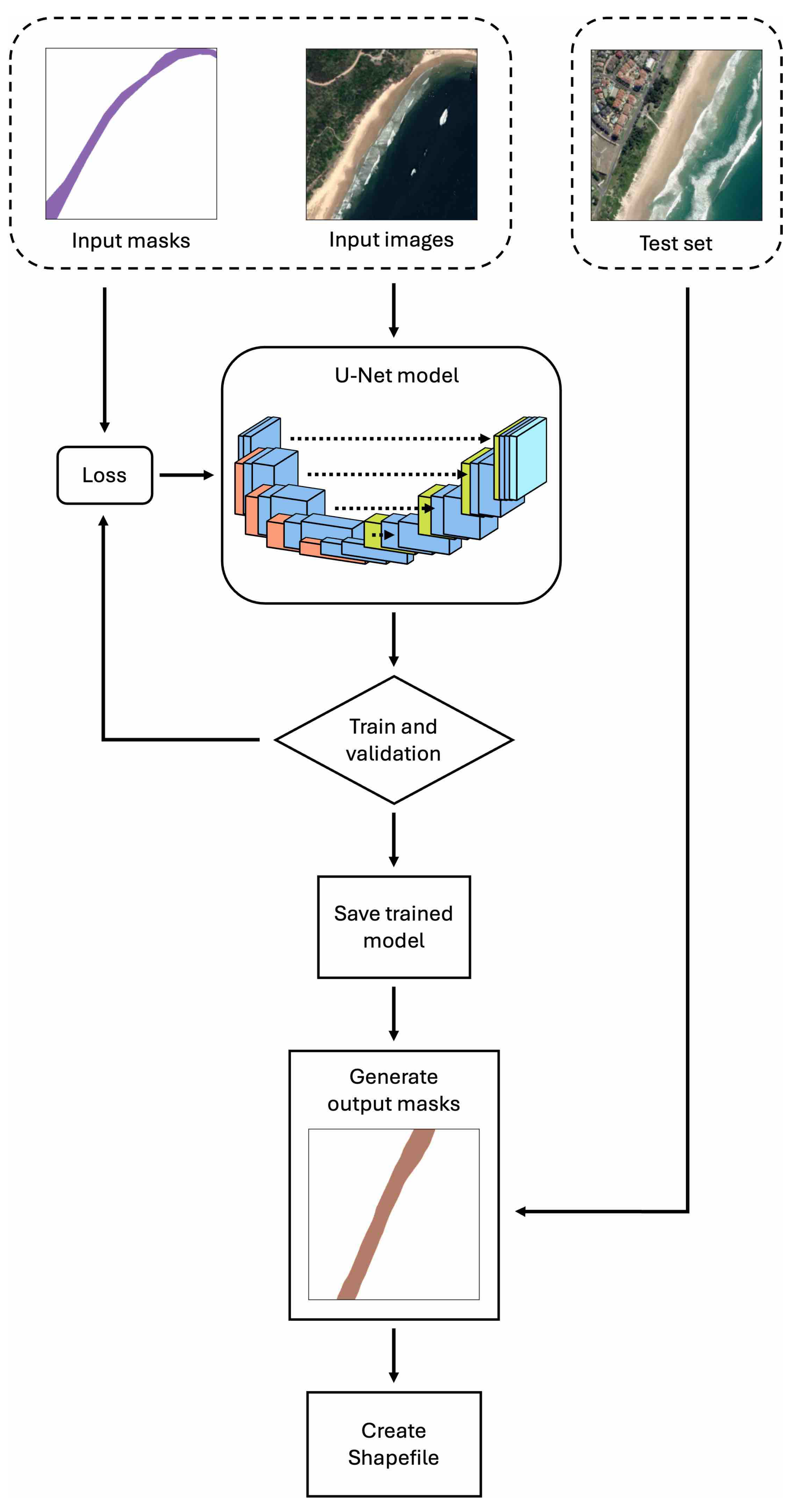
A flowchart of the pipeline is presented in Figure 3. The pipeline was constructed using PyTorch [29], an open-source DL library in Python. To perform the segmentation task, a DL model based on the U-Net architecture [30], which is a variant of CNNs, was employed. The U-Net features an encoder–decoder structure, as illustrated in Figure 4. The encoder consists of a series of convolutional layers followed by max-pooling layers. These blocks extract hierarchical features from the input image while progressively reducing its spatial dimensions through downsampling. Conversely, the decoder is composed of upsampling layers combined with convolutional layers. These blocks reconstruct the spatial resolution of the image. Another key element that concatenates or connects the layers of the decoder to their corresponding layers in the encoder is the skip connections. These connections allow the decoder to recover the fine spatial details lost during downsampling, while maintaining the learned features. The final layer of the U-Net architecture is a 1 × 1 convolutional layer, which generates the output binary segmentation map.
The U-Net model was implemented using the SMP (https://github.com/qubvel/segmentation_models.pytorch, accessed on 18 July 2024) [31] package. To balance a trade-off between model complexity and computational efficiency, the EfficientNet-B0 encoder [32] with pre-trained weights from ImageNet was chosen. The model was trained using stochastic gradient descent with an Adam optimizer [33], employing a learning rate of 10 4 and a weight decay of 10 6 . Training proceeded with a batch size of 128 for 500 epochs. During training, the model was optimised using the Dice loss function, a commonly utilised metric for image segmentation tasks. The model, once trained, was then applied to generate masks for all images, encompassing training, validation, and testing datasets, as well as those without masks. This corresponds to 6777 from the VIC state and 8950 from the NSW state. Following this step, Shapefiles were created from the produced masks.
Our experiments were conducted on a CSIRO high-performance accelerator computing cluster, Virga, consisting of Dual Xeon 36-core 8452Y CPUs with 512 GB RAM and NVIDIA Hopper H100 GPUs. The training time on a single node with 4 GPUs for the VIC dataset is ∼15.5 h and ∼19.3 h for the NSW dataset. The evaluation of the entire dataset took ∼9.9 min for VIC data and ∼11.5 min for NSW data.

2.2.2. Evaluation of the Model Performance

The resulting DL raster mask output predictions for each 512 × 512 image was vectorized and aggregated to create predicted beach polygons for evaluation. The overall performance of the U-Net DL model was assessed using the metric IoUdataset by comparing the performance across the training and validation datasets. IoUdataset is the average Intersection over Union (IoU) across the entire dataset and is defined as follows:
IoU dataset = 1 N i N IoU i ,
where N is the number of images in the dataset and IoUi is the IoU for the i-th image. The detailed definition of IoU will be defined subsequently. IoUdataset thus provides an aggregate measure of the model’s segmentation performance.
Additionally, three metrics are used to evaluate and compare the DL predicted beach polygons ( Y ^ ) to the citizen-science-drawn polygons (Y) in OSM. While the processing was performed on raster tiles, the evaluation was on the aggregated vectorisation of the predicted tiles, i.e., polygon beach shapes. The first evaluation metric is the commonly used IoU or Jaccard index. The other two metrics are similar, representing the intersection over the citizen-science-drawn polygons (IoY) and the intersection over the DL predicted polygons (Io Y ^ ). These are formulated as
IoU = area ( Y Y ^ ) area ( Y Y ^ ) ,
IoY = area ( Y Y ^ ) area ( Y ) ,
Io Y ^ = area ( Y Y ^ ) area ( Y ^ ) .
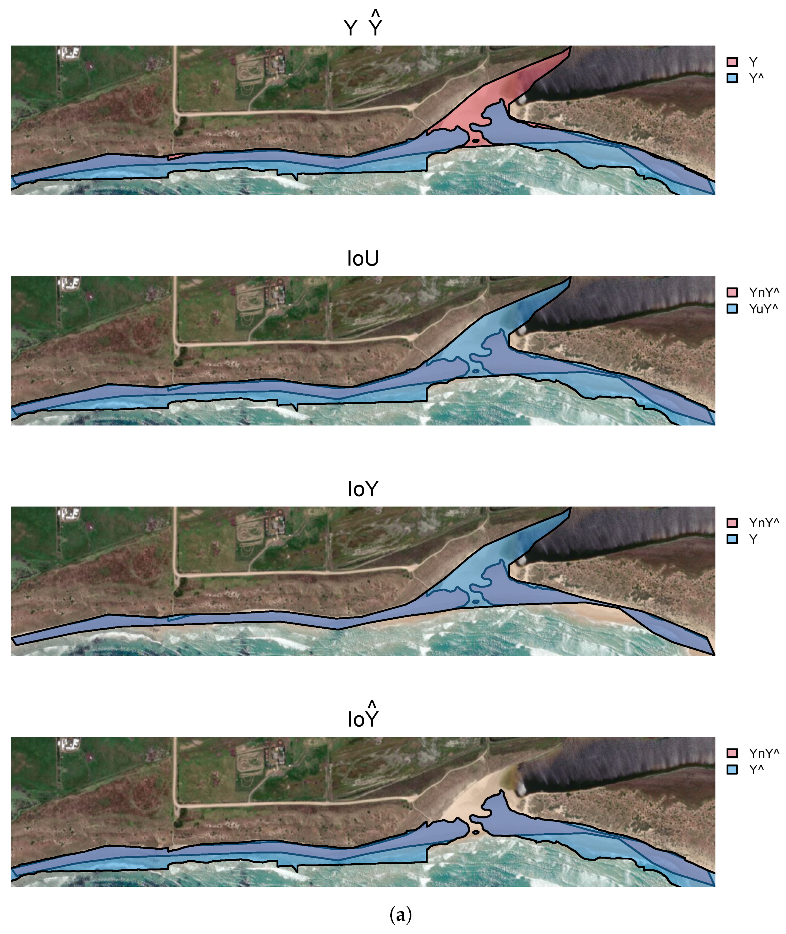
The computed regions for the three evaluation metrics and how the area of the polygons overlap for Y and Y ^ are illustrated in Figure 5.
IoU is the ratio of the area of overlap over the area of union. It compares how well the DL predicted polygons exactly align with the citizen-science-drawn polygons. Notably, errors in citizen-science-drawn representation of beaches can lead to omissions of parts of the beach, extensions into the swash zone or dunes, or instances where DL-predicted polygons extend into neighboring beaches.
IoY is the ratio of the area of overlap over the area of the citizen-science-drawn polygon and indicates whether DL can at least cover the area of the citizen-science-drawn polygon. Io Y ^ is the ratio of the area of overlap over the area of the DL predicted polygon and indicates if DL can predict areas outside of the citizen-science-drawn polygon, i.e., find new parts of the beach not drawn by people. The range of values is from 0 to 1, where the higher the value, the larger the overlapping area and a value of 1 indicates a perfect match. Io Y ^ can exceed 1, indicating that new areas are mapped by the DL model.

3. Results

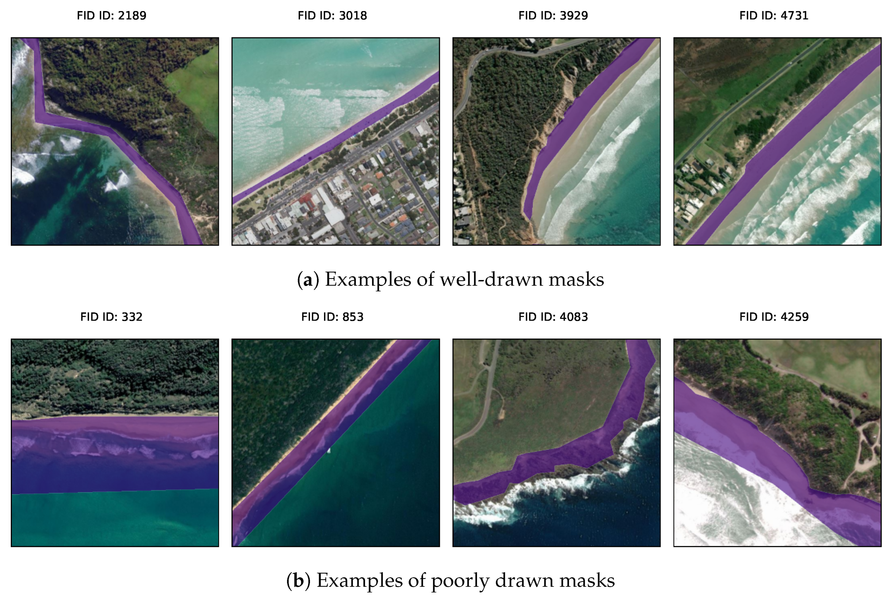
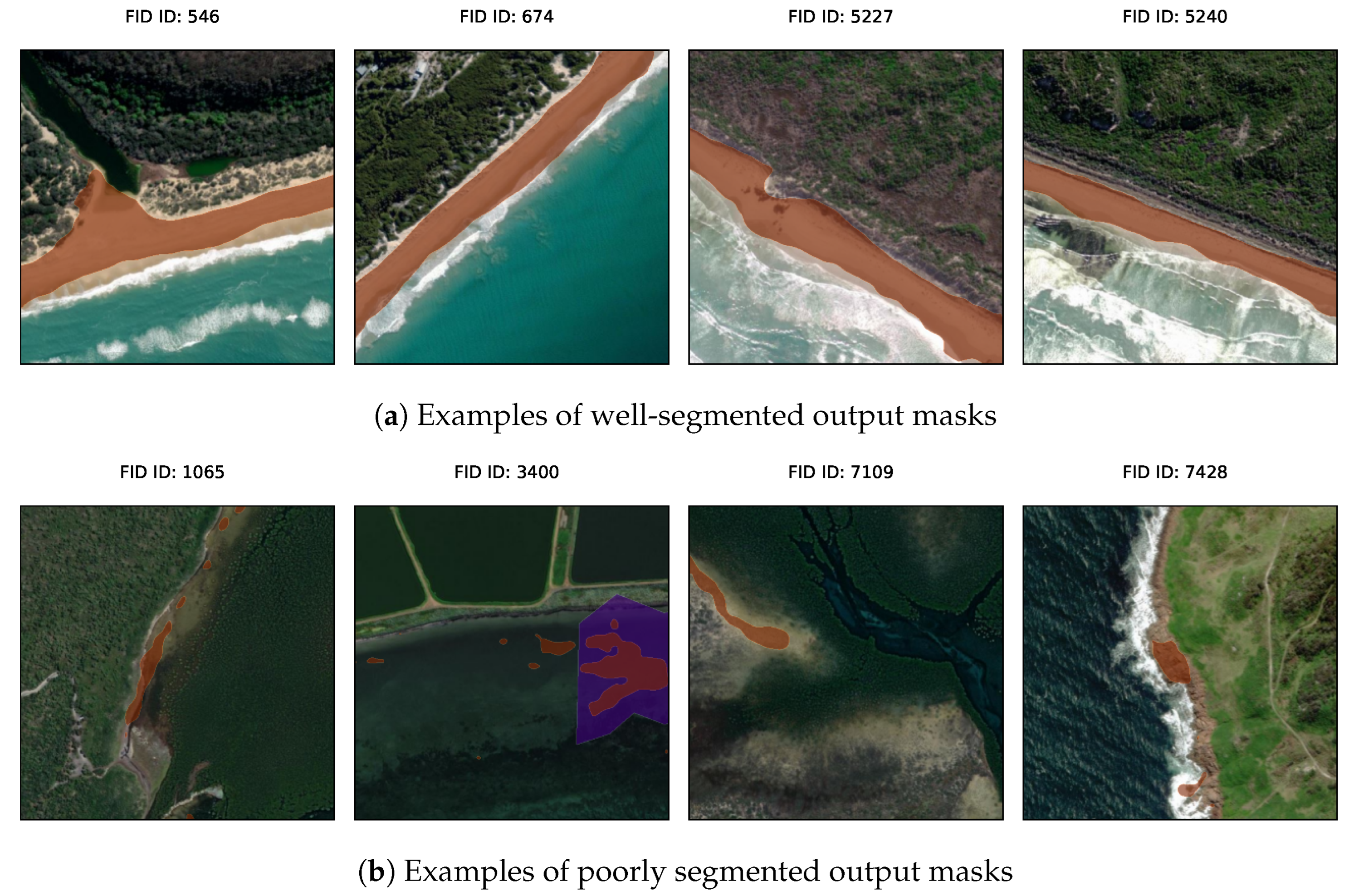
Images with citizen-science-drawn beach polygons as approximate ground truth masks are used to train the supervised DL model. Examples of well-drawn and poorly drawn masks are illustrated in Figure 6. Although a substantial number of masks feature coverage that is adequately drawn (Figure 6a), some exhibit shortcomings, such as being overly narrow/broad or being inaccurately drawn on cliffs (Figure 6b). Figure 7 presents predictions generated by the DL model, depicting images captured along the coast of VIC with their corresponding segmented predictions for the test dataset.
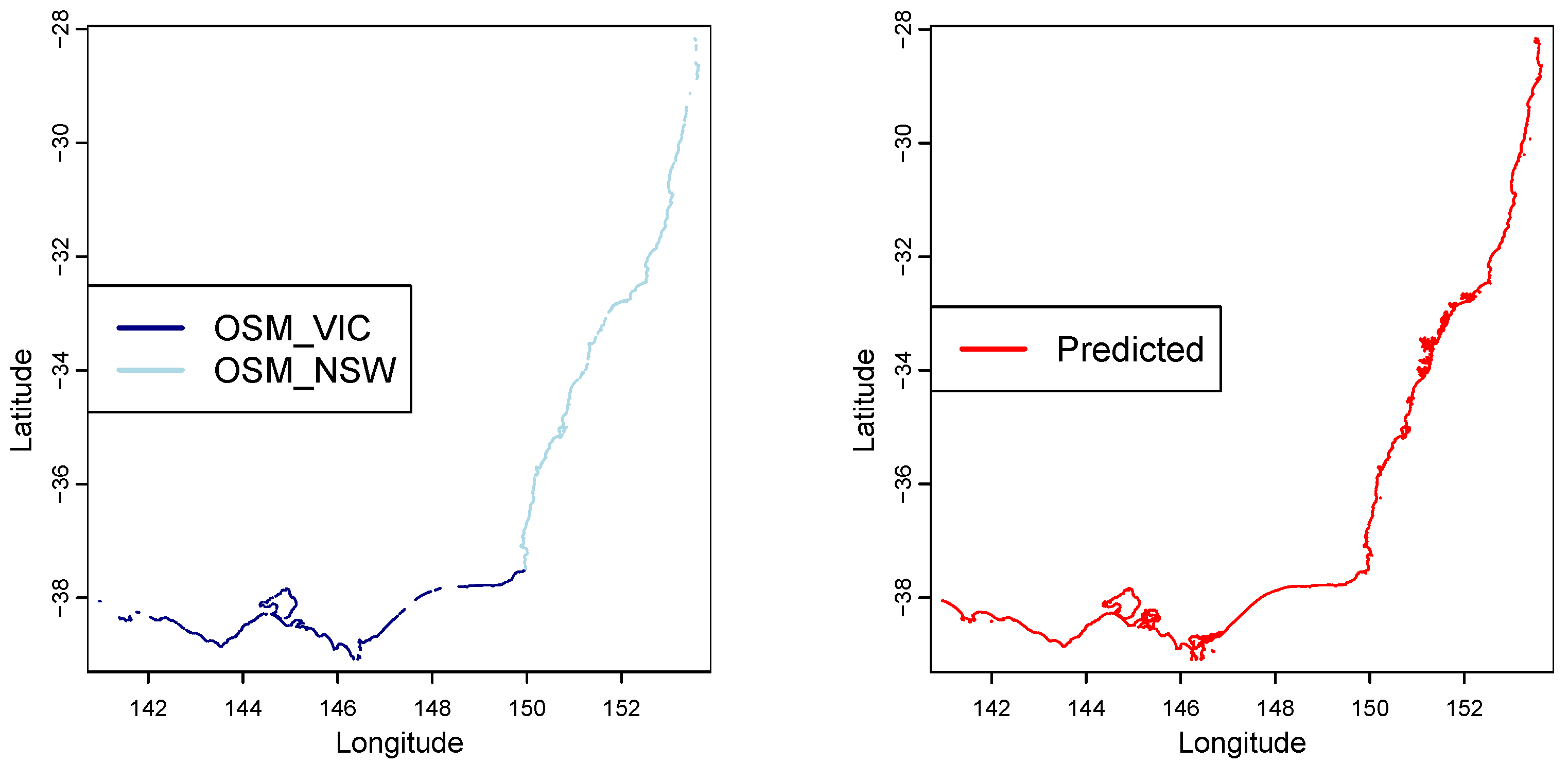
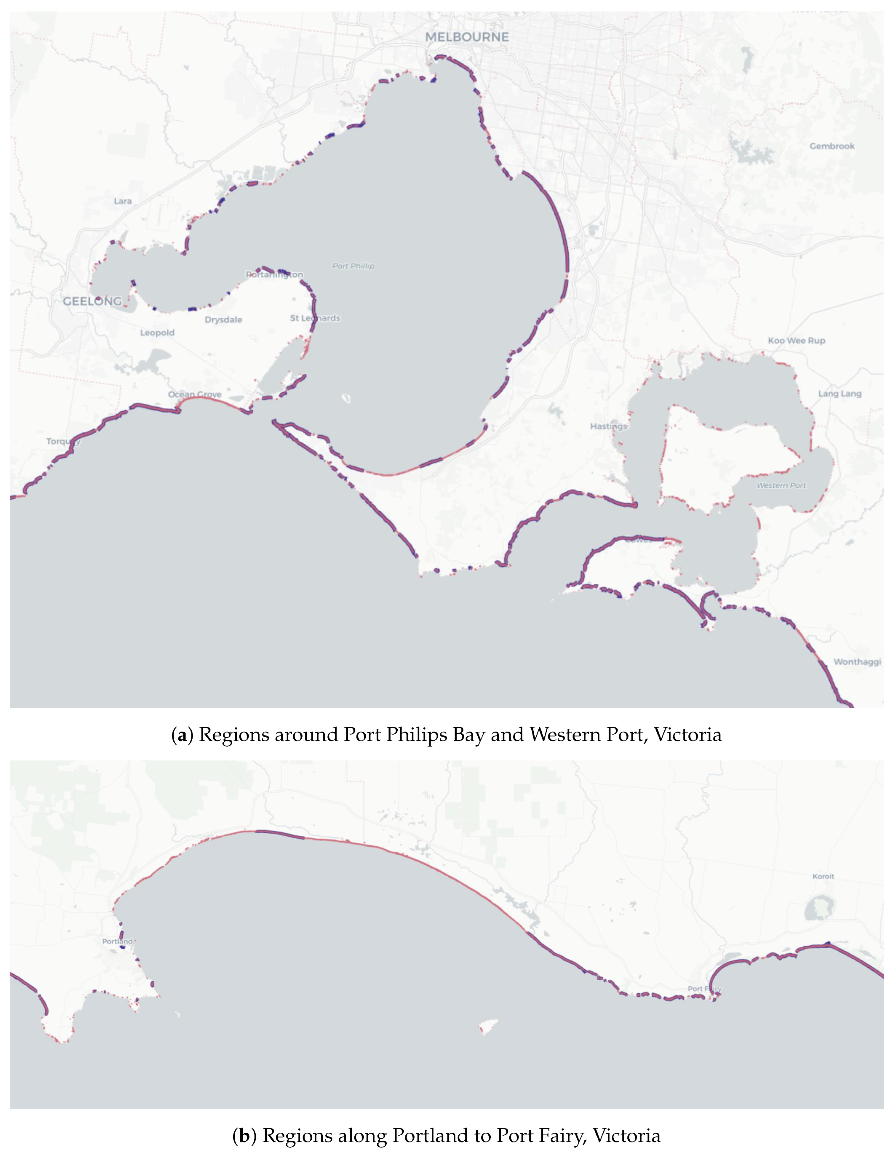
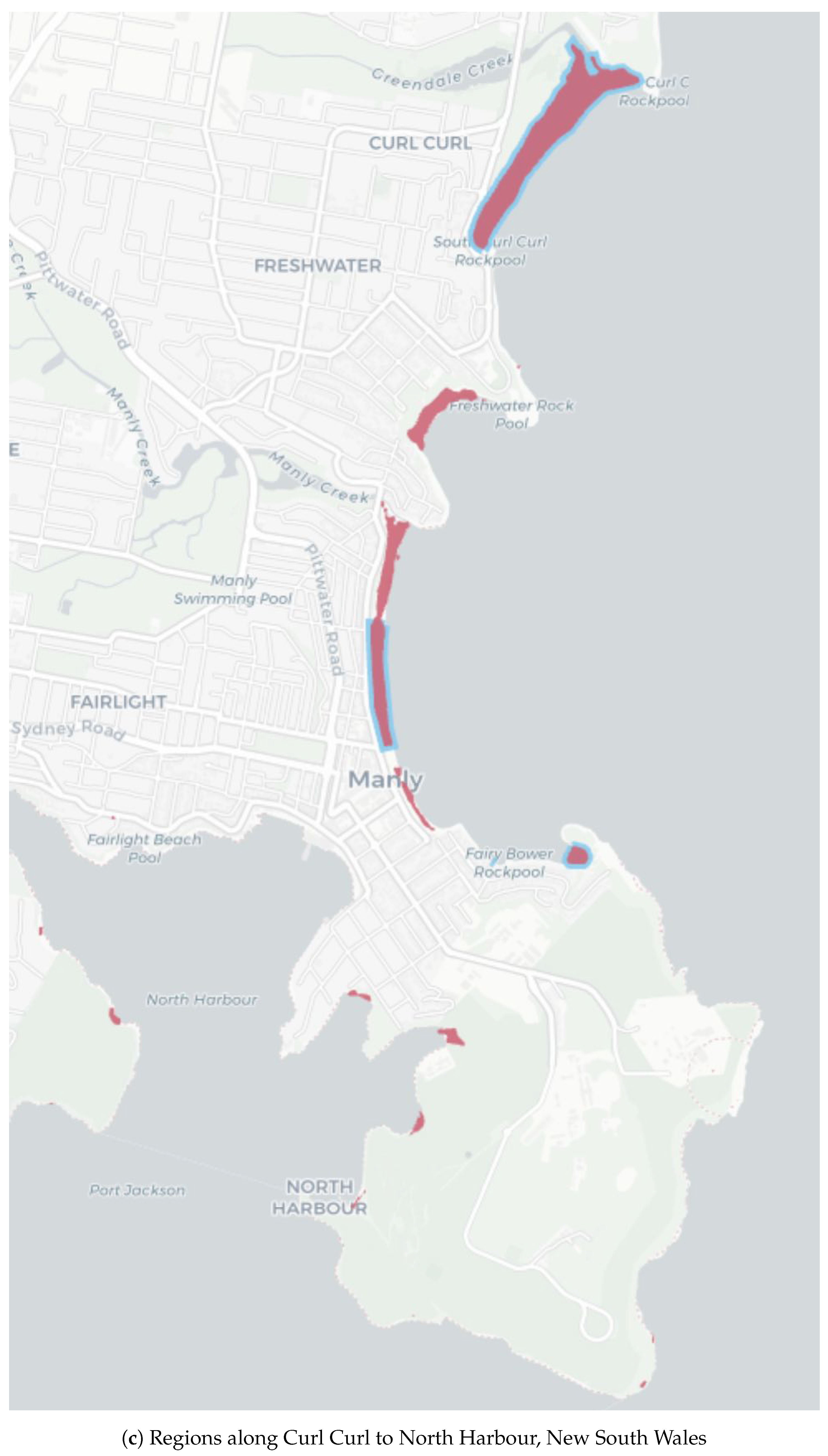
The broad-scale maps of beach polygons from OSM and DL predictions for the entire coast of VIC and NSW are shown in Figure 2. These beach polygons, provided in Shapefiles format, can be uploaded to NationalMap (https://nationalmap.gov.au, accessed on 14 September 2024) for further analysis. Figure 8 displays zoomed-in views of selected coastal regions in VIC (Figure 8a,b) and NSW (Figure 8c), as exported using NationalMap. The OSM beach polygons are depicted in shades of blue and DL predictions are highlighted in red. The DL model can identify previously unmapped sandy areas, such as those in Western Port, VIC (Figure 8a), and smaller beaches around North Harbour, NSW (Figure 8c). Nonetheless, as mentioned before, the model also exhibits some inaccuracies, including the incorrect inclusion of cliffs, as can be identified in the bottom center of Figure 8b.
Table 1 compares the IoU between the training and validation sets for the two model setups, one trained on VIC data and the other on NSW data. It provides an overview of the performance differences between the training and validation sets and assesses the model’s ability to perform on new data. The IoU values for both sets were similar. For the DL model using VIC data, the IoU was 0.69 for the training set and 0.70 for the validation set. For the DL model using NSW data, the IoU was 0.72 and 0.74 for the training and validation sets, respectively. This suggests that the model is likely to generalise well to new unseen datasets. However, it is important to note that this assessment might not fully reflect the model’s performance. As previously mentioned, the ground truth masks used for evaluation are manually labelled and may contain inaccuracies. These labelling errors could affect the accuracy of the IoU metrics.
A summary of statistics derived from model evaluations for beach polygons across VIC and NSW is presented in Table 2. For examples of mapped beach polygons along with the evaluation metrics for selected beaches in VIC and NSW, refer to Figure 5a and Figure 5b, respectively. In addition to the statistics provided in the table, Figure 9 shows the kernel density plot, which provides a smooth estimate of the data distribution. Figure 10 displays the corresponding empirical cumulative distribution function (eCDF), which illustrates the cumulative probability distribution of the metrics. The eCDF plot helps visualize the proportion of beaches within certain performance thresholds.
There were a total of 556 beaches in VIC and 593 OSM-downloaded beaches available for evaluation, representing areas of 47.43 and 74.54 square kilometers, respectively. For VIC, the trained DL model predicted several thousand smaller beach polygons (e.g., in Figure 7a), and extended the mapped area by approximately 10 square kilometers. Figure 1 highlights some of the gaps in the training dataset, such as Western Port and parts of Ninety Mile Beach due to limitations in the OSM extraction, which were filled in by the DL predictions.
In NSW, the VIC-trained DL model predicted many thousands of smaller beaches compared with the locally trained NSW model. However, this represented a smaller area than the training dataset. One possible reason for this discrepancy is that the model was trained on more of the dry parts of the beach, while untrained OSM-drawn outlines extended into the wet swash zone.
When using a model trained on data from the same state for predictions in that state, the NSW-trained model (NSW Y NSW Y ^ ) performs better, with a mean IoU of 0.76 and a median IoU of 0.85. In contrast, the VIC-trained model applied to VIC (VIC Y VIC Y ^ ) had a mean IoU of 0.66 and a median IoU of 0.78. A higher percentage of beaches in NSW reached an IoU of 0.7 or higher compared with those in VIC, as seen in Figure 9 and Figure 10. This suggests that, on average, the overlap between DL predicted and citizen-science-drawn beach polygons is closer for NSW, indicating higher accuracy in these predictions.
Similarly for IoY, NSW outperformed VIC with higher mean and median values of 0.90 and 0.96, respectively, compared with VIC with 0.88 and 0.96, respectively. These metrics demonstrate the model’s effectiveness in covering the areas delineated by citizen science experts, with NSW showing greater coverage. Meanwhile, the mean Io Y ^ in VIC was 2.93 with a median of 1.08, whereas NSW had lower values of 1.35 and 1.05, respectively. The higher Io Y ^ values for the VIC-trained model indicate that the model predicted beyond the citizen-science-drawn areas more frequently than those for NSW.
Overall, predictions conducted using a model trained on data from the same state performed significantly better than when trained on data from a different state. This was prominently evident in NSW, where the IoU was more than twice as low when using the model trained on VIC data. Additionally, high IoU and IoY values were also less common, as shown in Figure 9 and Figure 10.

4. Discussion

This study serves as a proof of concept for segmenting beach images in two Australian states, VIC and NSW, utilising supervised DL techniques. We provide the dataset, comprising image extents and corresponding polygon masks, used to train the DL model, along with the trained model itself, which can be utilised for further evaluation or refined through fine-tuning. The evaluation process is relatively quick, taking approximately 10 min to predict 8000 samples on our system. Additionally, the predictions generated from the DL are available in Shapefiles format, which can be loaded to NationalMap (https://nationalmap.gov.au, accessed on 22 September 2024).
Overall, the DL model demonstrates a promising avenue to segmenting sandy areas in beach images, despite encountering some limitations. Although the model effectively segments sandy regions along the coast (Figure 7a), it occasionally encounters challenges akin to those present in the citizen-science-drawn masks, such as erroneously incorporating cliff areas (Figure 7b). Additionally, it displays an oversensitivity to details resembling sandy areas, leading to mistaken segmentation. When considering that coastal change (erosion/accretion) is often measured as an onshore/offshore displacement of the shoreline (e.g., [12]), the commonly used IoU metric has its limitations in model evaluation. It compares areas and may not fully capture the dynamic and highly variable nature of the shoreline (e.g., runup and storm bite), which is challenging to map from aerial imagery. In this analysis, we not only map the shoreline but also the backshore (e.g., vegetation or dune lines), which is more consistently identifiable and stable compared with the highly variable shoreline. This approach allows for the tracking of long-term coastal changes closer to coastal assets by also focusing on the stable backshore of the beach outline, and the IoU metric evaluates the area between shoreline and backshore.
NSW exhibits a higher IoU score compared with VIC, possibly due to the greater visual similarity among beach images in NSW. The Io Y ^ score is larger for VIC, suggesting the algorithm has predicted unmapped beaches or there is potential over-estimation of the model in this region. Furthermore, when evaluating the models on different regions, their performance is notably worse compared with evaluations within the same region, indicating a need for fine-tuning specific to local regions. This also indicates the high dependency of local training data. Hence, we recommend fine-tuning the model for individual regions or custom datasets to improve segmentation accuracy. Here, we would expect that the training models would also perform poorly for other regions in Australia, such as the iron-rich red sand of Western Australia. We would also expect that it could perform poorly for international locations, such as the black volcanic sand of Pacific Island archipelago nation Vanuatu.
Future work will involve integrating beach images from diverse states into the DL training process. Similarly, incorporating data augmentation, such as geometric transformations, will introduce more variations. This will enable the DL model to adapt to and learn from the diverse range of image variations, thus enhancing its robustness. In the training dataset, untrained OSM mappers may have faced difficulties distinguishing sandy backshore areas from features such as bare dunes or coastal roads. Variability in waterlines, influenced by tides, swash excursions, and the water table, can further affect mapping accuracy depending on the timing of the imagery. These issues will undoubtedly influence any model designed to predict future beach outlines. Further post processing incorporating geomorphology such as steep cliffs from elevation datasets to mask erroneous sand coloured cliffs can be employed to improve the datasets. Shoreline land–sea mask could also be used to improve the datasets. As previously noted, the presence of cliffs can pose a challenge for the DL model. Introducing multi-class segmentation, with cliffs as an additional class to be identified, could potentially assist the DL model in distinguishing sandy areas more accurately. Furthermore, exploring alternative DL architectures may offer avenues for improving performance.
The precise mapping of beach extents allows for more accurate assessments of coastal vulnerability. This information is crucial for predicting, adapting, and mitigating the impacts of sea-level rise, storm surges, and coastal erosion. Additionally, real-time updates of beach outlines following extreme weather events would be valuable for investigating their impacts. By identifying at-risk areas, policymakers and coastal managers can develop targeted adaptation strategies to protect infrastructure, ecosystems, and communities. Beaches provide habitats for various species, including nesting sites for endangered sea turtles and shorebirds. The methods demonstrated in the paper should be considered in context tracking how beach outlines have changed in historical aerial images, and how this could support biodiversity monitoring. The methods presented here use global datasets, hence, could help facilitate international analysis.

5. Conclusions

In this study, we applied supervised deep learning to segment beach images at the regional scale for two Australian states, Victoria (VIC) and New South Wales (NSW), with coastlines on the order of 2000–2500 km long. Generally, the model demonstrates the capability to generate reasonably accurate segmentation and rapid predictions. However, it exhibits certain limitations, including misclassifying cliffs and being overly sensitive to fine details, resulting in inaccuracies in the generated maps. Comparative analysis indicates differences in performance between VIC and NSW, with NSW showing better scores. Cross-region evaluations highlight the necessity for region-specific fine-tuning to improve segmentation accuracy. Overall, the analysis shows the potential for a deep learning approach to replicate and build upon citizen science mapping beaches, highlighting the need for local training dataset to work towards an accurate representation of beach outlines at continental and global scales.
Accurately mapping this geomorphology is essential for coastal hazard and risk assessments, particularly when modelling the future impacts of sea level rise. A key consideration from this study is the advantage of mapping beach outlines instead of just the shoreline, as it captures the location of backshore features such as vegetated dunes, cliffs, and defence structures. These beach outlines provide an improved estimate of the geomorphology of potentially erodible soft beach areas, which act as a natural buffer to the backshore. However, the method still lacks estimates of beach erodible volume, depth to bedrock or consolidated substrate, and offshore sediment supply—critical factors for a more comprehensive understanding of coastal change at the local scale [34,35,36,37].
Citizen science has proven useful in contributing to beach and coastal datasets across Australia, predominantly at individual sites [38,39,40]. In this study, we further demonstrate the value of citizen science at a national scale, highlighting its potential for broader impact and emphasising the need to promote greater participation. The OSM initiative is a global effort, and, as such, the data and methodology presented in this study should be considered applicable on a global scale, with potential relevance for use in other regions around the world. The model and datasets are made openly available to support and encourage further coastal mapping activities, and their application to coastal management. The model and datasets are made openly available to support and encourage further coastal mapping activities, and their application to coastal management.

Author Contributions

Conceptualization, S.Y.Y. and J.O.; methodology, S.Y.Y. and J.O.; software, S.Y.Y. and J.O.; validation, S.Y.Y.; formal analysis, S.Y.Y. and J.O.; investigation, S.Y.Y. and J.O.; data curation, J.O.; writing—original draft preparation, S.Y.Y. and J.O.; writing—review and editing, S.Y.Y., J.O., R.G. and D.L.; visualization, S.Y.Y. and J.O.; funding acquisition, J.O. All authors have read and agreed to the published version of the manuscript.

Funding

This work has been funded by the Australian Climate Service (ACS).

Data Availability Statement

The data presented in this study are available on the CSIRO Data Access Portal at http://hdl.handle.net/102.100.100/636518 (accessed on 25 July 2024), further inquiries can be directed to the corresponding author/s. Map data copyrighted OpenStreetMap contributors and available from https://www.openstreetmap.org (accessed on 20 June 2024). The original code from sandybeachmapping_dl is openly available on the CSIRO Data Access Portal at http://hdl.handle.net/102.100.100/636534 (accessed on 26 July 2024).

Acknowledgments

We would like to acknowledge the support of Brint Gardner and the CSIRO Information Management & Technology Scientific Computing Collaboration Projects program. We also acknowledge the contribution of the work experience students and citizen scientist who have contributed mapped beaches in OSM. This research made use of the Python libraries including open source packages including PyTorch [29] and SMP [31], as well as R packages such as OpenStreetMap, osmdata [28], terra [26].

Conflicts of Interest

The authors declare no conflicts of interest.

References

  1. James, R.J. From beaches to beach environments: Linking the ecology, human-use and management of beaches in Australia. Ocean Coast. Manag. 2000, 43, 495–514. [Google Scholar] [CrossRef]
  2. Defeo, O.; McLachlan, A.; Schoeman, D.S.; Schlacher, T.A.; Dugan, J.; Jones, A.; Lastra, M.; Scapini, F. Threats to sandy beach ecosystems: A review. Estuar. Coast. Shelf Sci. 2009, 81, 1–12. [Google Scholar] [CrossRef]
  3. Rocha, C.; Antunes, C.; Catita, C. Coastal indices to assess sea-level rise impacts—A brief review of the last decade. Ocean Coast. Manag. 2023, 237, 106536. [Google Scholar] [CrossRef]
  4. Vousdoukas, M.I.; Ranasinghe, R.; Mentaschi, L.; Plomaritis, T.A.; Athanasiou, P.; Luijendijk, A.; Feyen, L. Reply to: Sandy beaches can survive sea-level rise. Nat. Clim. Chang. 2020, 10, 996–997. [Google Scholar] [CrossRef]
  5. Konlechner, T.M.; Kennedy, D.M.; O’Grady, J.J.; Leach, C.; Ranasinghe, R.; Carvalho, R.C.; Luijendijk, A.P.; McInnes, K.L.; Ierodiaconou, D. Mapping spatial variability in shoreline change hotspots from satellite data; a case study in southeast Australia. Estuar. Coast. Shelf Sci. 2020, 246, 107018. [Google Scholar] [CrossRef]
  6. Nanson, R.; Bishop-Taylor, R.; Sagar, S.; Lymburner, L. Geomorphic insights into Australia’s coastal change using a national dataset derived from the multi-decadal Landsat archive. Estuar. Coast. Shelf Sci. 2022, 265, 107712. [Google Scholar] [CrossRef]
  7. Short, A.D. Australian Beach Systems—Nature and Distribution. J. Coast. Res. 2006, 22, 11–27. [Google Scholar] [CrossRef]
  8. Sagar, S.; Roberts, D.; Bala, B.; Lymburner, L. Extracting the intertidal extent and topography of the Australian coastline from a 28 year time series of Landsat observations. Remote Sens. Environ. 2017, 195, 153–169. [Google Scholar] [CrossRef]
  9. Vos, K.; Deng, W.; Harley, M.D.; Turner, I.L.; Splinter, K.D.M. Beach-face slope dataset for Australia. Earth Syst. Sci. Data 2022, 14, 1345–1357. [Google Scholar] [CrossRef]
  10. Luijendijk, A.; Hagenaars, G.; Ranasinghe, R.; Baart, F.; Donchyts, G.; Aarninkhof, S. The State of the World’s Beaches. Sci. Rep. 2018, 8, 6641. [Google Scholar] [CrossRef]
  11. Vos, K.; Harley, M.D.; Splinter, K.D.; Simmons, J.A.; Turner, I.L. Sub-annual to multi-decadal shoreline variability from publicly available satellite imagery. Coast. Eng. 2019, 150, 160–174. [Google Scholar] [CrossRef]
  12. Bishop-Taylor, R.; Nanson, R.; Sagar, S.; Lymburner, L. Mapping Australia’s dynamic coastline at mean sea level using three decades of Landsat imagery. Remote Sens. Environ. 2021, 267, 112734. [Google Scholar] [CrossRef]
  13. Zhou, X.; Wang, J.; Zheng, F.; Wang, H.; Yang, H. An Overview of Coastline Extraction from Remote Sensing Data. Remote Sens. 2023, 15, 4865. [Google Scholar] [CrossRef]
  14. Warrick, J.A.; Buscombe, D.; Vos, K.; Bryan, K.R.; Castelle, B.; Cooper, J.A.G.; Harley, M.D.; Jackson, D.W.T.; Ludka, B.C.; Masselink, G.; et al. Coastal shoreline change assessments at global scales. Nat. Commun. 2024, 15, 2316. [Google Scholar] [CrossRef] [PubMed]
  15. Gao, J.; Kennedy, D.M.; McSweeney, S. Decadal changes in vegetation cover within coastal dunes at the regional scale in Victoria, SE Australia. J. Environ. Manag. 2024, 351, 119622. [Google Scholar] [CrossRef]
  16. O’Grady, J.G.; McInnes, K.L.; Hemer, M.A.; Hoeke, R.K.; Stephenson, A.G.; Colberg, F. Extreme Water Levels for Australian Beaches Using Empirical Equations for Shoreline Wave Setup. J. Geophys. Res. Ocean. 2019, 124, 5468–5484. [Google Scholar] [CrossRef]
  17. Vitousek, S.; Barnard, P.L.; Fletcher, C.H.; Frazer, N.; Erikson, L.; Storlazzi, C.D. Doubling of coastal flooding frequency within decades due to sea-level rise. Sci. Rep. 2017, 7, 1399. [Google Scholar] [CrossRef]
  18. Yuan, X.; Shi, J.; Gu, L. A review of deep learning methods for semantic segmentation of remote sensing imagery. Expert Syst. Appl. 2021, 169, 114417. [Google Scholar] [CrossRef]
  19. Arellano-Verdejo, J.; Santos-Romero, M.; Lazcano-Hernandez, H.E. Use of semantic segmentation for mapping Sargassum on beaches. PeerJ 2022, 10, e13537. [Google Scholar] [CrossRef]
  20. Buscombe, D.; Goldstein, E.B. A Reproducible and Reusable Pipeline for Segmentation of Geoscientific Imagery. Earth Space Sci. 2022, 9, e2022EA002332. [Google Scholar] [CrossRef]
  21. Chang, L.; Chen, Y.T.; Wu, M.C.; Alkhaleefah, M.; Chang, Y.L. U-Net for Taiwan Shoreline Detection from SAR Images. Remote Sens. 2022, 14, 5135. [Google Scholar] [CrossRef]
  22. Aghdami-Nia, M.; Shah-Hosseini, R.; Rostami, A.; Homayouni, S. Automatic coastline extraction through enhanced sea-land segmentation by modifying Standard U-Net. Int. J. Appl. Earth Obs. Geoinf. 2022, 109, 102785. [Google Scholar] [CrossRef]
  23. Scala, P.; Manno, G.; Ciraolo, G. Semantic segmentation of coastal aerial/satellite images using deep learning techniques: An application to coastline detection. Comput. Geosci. 2024, 192, 105704. [Google Scholar] [CrossRef]
  24. Wernette, P.A.; Buscombe, D.D.; Favela, J.; Fitzpatrick, S.; Goldstein, E.; Enwright, N.M.; Dunand, E. Coast Train–Labeled Imagery for Training and Evaluation of Data-Driven Models for Image Segmentation; US Geological Survey: Tallahassee, FL, USA, 2022. [CrossRef]
  25. OpenStreetMap Contributors. Planet Dump Retrieved from https://planet.osm.org. 2017. Available online: https://www.openstreetmap.org (accessed on 20 June 2024).
  26. Hijmans, R.J. Terra: Spatial Data Analysis. 2024. R Package Version 1.7-80. Available online: https://rspatial.github.io/terra/ (accessed on 20 June 2024).
  27. Australian Bureau of Statistics. Digital Boundary Files. ABS, July 2021–June 2026. Available online: https://www.abs.gov.au/statistics/standards/australian-statistical-geography-standard-asgs-edition-3/jul2021-jun2026/access-and-downloads/digital-boundary-files (accessed on 6 June 2024).
  28. Padgham, M.; Rudis, B.; Lovelace, R.; Salmon, M. osmdata. J. Open Source Softw. 2017, 2, 305. [Google Scholar] [CrossRef]
  29. Paszke, A.; Gross, S.; Massa, F.; Lerer, A.; Bradbury, J.; Chanan, G.; Killeen, T.; Lin, Z.; Gimelshein, N.; Antiga, L.; et al. PyTorch: An Imperative Style, High-Performance Deep Learning Library. In Proceedings of the Advances in Neural Information Processing Systems, Vancouver, BC, Canada, 8–14 December 2019; Wallach, H., Larochelle, H., Beygelzimer, A., d’Alché-Buc, F., Fox, E., Garnett, R., Eds.; Curran Associates, Inc.: Nice, France, 2019; Volume 32. [Google Scholar]
  30. Ronneberger, O.; Fischer, P.; Brox, T. U-Net: Convolutional Networks for Biomedical Image Segmentation. In Proceedings of the Medical Image Computing and Computer-Assisted Intervention—ICCAI 2015, Munich, Germany, 5–9 October 2015; Navab, N., Hornegger, J., Wells, W.M., Frangi, A.F., Eds.; Springer International Publishing: Cham, Switzerland, 2015; pp. 234–241. [Google Scholar]
  31. Iakubovskii, P. Segmentation Models Pytorch. 2019. Available online: https://github.com/qubvel/segmentation_models.pytorch (accessed on 18 July 2024).
  32. Tan, M.; Le, Q. EfficientNet: Rethinking Model Scaling for Convolutional Neural Networks. In Proceedings of the 36th International Conference on Machine Learning, Long Beach, CA, USA, 9–15 June 2019; Volume 97, pp. 6105–6114. [Google Scholar]
  33. Kingma, D.P.; Ba, J. Adam: A Method for Stochastic Optimization. In Proceedings of the 3rd International Conference on Learning Representations, ICLR 2015, San Diego, CA, USA, 7–9 May 2015; Conference Track Proceedings. Bengio, Y., LeCun, Y., Eds.; [Google Scholar]
  34. Wright, L.; Short, A. Morphodynamic variability of surf zones and beaches: A synthesis. Mar. Geol. 1984, 56, 93–118. [Google Scholar] [CrossRef]
  35. Gallop, S.L.; Kennedy, D.M.; Loureiro, C.; Naylor, L.A.; Muñoz-Pérez, J.J.; Jackson, D.W.; Fellowes, T.E. Geologically controlled sandy beaches: Their geomorphology, morphodynamics and classification. Sci. Total Environ. 2020, 731, 139123. [Google Scholar] [CrossRef]
  36. Short, A.D. Australian Coastal Systems: Beaches, Barriers and Sediment Compartments, 1st ed.; Coastal Research Library, Springer International Publishing AG: Cham, Switzerland, 2020; Volume 32, pp. 1–1241. [Google Scholar] [CrossRef]
  37. Anthony, E.J.; Aagaard, T. The lower shoreface: Morphodynamics and sediment connectivity with the upper shoreface and beach. Earth-Sci. Rev. 2020, 210, 103334. [Google Scholar] [CrossRef]
  38. Harley, M.D.; Kinsela, M.A.; Sánchez-García, E.; Vos, K. Shoreline change mapping using crowd-sourced smartphone images. Coast. Eng. 2019, 150, 175–189. [Google Scholar] [CrossRef]
  39. Pucino, N.; Kennedy, D.M.; Carvalho, R.C.; Allan, B.; Ierodiaconou, D. Citizen science for monitoring seasonal-scale beach erosion and behaviour with aerial drones. Sci. Rep. 2021, 11, 3935. [Google Scholar] [CrossRef]
  40. Ierodiaconou, D.; Kennedy, D.M.; Pucino, N.; Allan, B.M.; McCarroll, R.J.; Ferns, L.W.; Carvalho, R.C.; Sorrell, K.; Leach, C.; Young, M. Citizen science unoccupied aerial vehicles: A technique for advancing coastal data acquisition for management and research. Cont. Shelf Res. 2022, 244, 104800. [Google Scholar] [CrossRef]
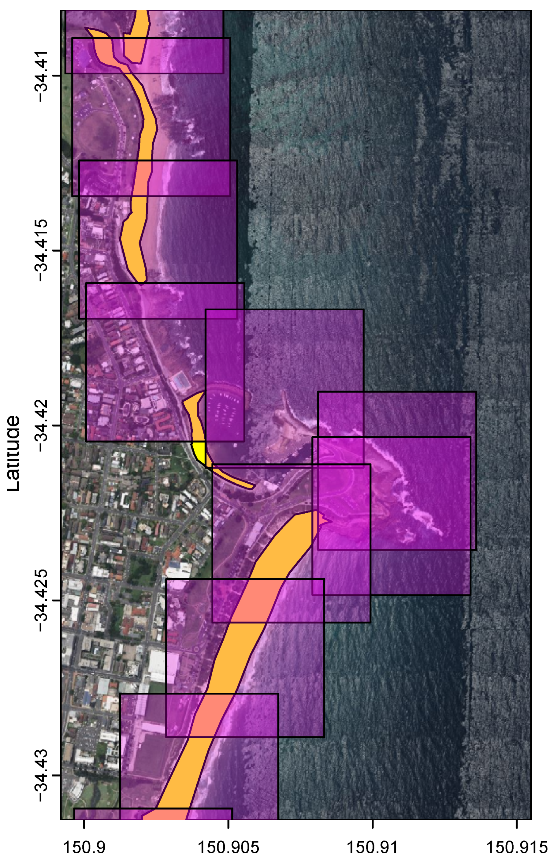
Figure 1. Example of image tiling near Wollongong, New South Wales. Purple squares are 512 m × 512 m image tiles and yellow polygons indicate OSM beach polygons.
Remotesensing 16 03534 g001
Figure 2. Map of OSM beaches used to train the model. (Left) Beach polygons for Victoria (VIC) and New South Wales (NSW) in blue and cyan. (Right) Regions mapped by the deep learning model in red.
Remotesensing 16 03534 g002
Figure 3. A flowchart of the pipeline for binary segmentation of sandy beaches.
Remotesensing 16 03534 g003
Figure 4. A diagram of the U-Net architecture.
Remotesensing 16 03534 g004
Figure 5. Examples of model evaluation for deep learning predicted and citizen-science-drawn beach polygons. From top to bottom in (a) or from left to right in (b): citizen-science-drawn polygons Y and predicted polygons Y ^ , Intersection over Union (IoU), intersection over the citizen-science-drawn polygons (IoY), and intersection over the deep learning predicted polygons (Io Y ^ ). The numerator and denominator of the three evaluation metrics are in red and blue, respectively. Purple indicates the overlap between red and blue regions. (a) Belfast Coastal Reserve, Tower Hill, Victoria (centroid 142.3656 E 38.34931 S, OSM ID = 9278056). (b) Brighton Beach, Wollongong, New South Wales (centroid 150.9042 E 34.42044 S, OSM ID = 257204435).
Remotesensing 16 03534 g005aRemotesensing 16 03534 g005b
Figure 6. Examples of beach images along the Victoria coast from the training dataset with their corresponding approximate ground truth masks in purple.
Remotesensing 16 03534 g006
Figure 7. Examples of beach images along the Victoria coast from the test dataset with their corresponding predicted output masks in orange. The approximate ground truth masks are provided in purple where available.
Remotesensing 16 03534 g007
Figure 8. Maps created by loading Shapefiles into NationalMap (https://nationalmap.gov.au, accessed on 14 September 2024). The outlines of citizen-science-drawn OSM beaches are depicted in shades of blue, while the predicted regions from the deep learning model are highlighted in red. The thickness of the mapped regions is intentionally increased to improve visual clarity.
Remotesensing 16 03534 g008aRemotesensing 16 03534 g008b
Figure 9. Kernel density plots with a bandwidth of 0.01 for Intersection over Union (IoU), intersection over the citizen-science-drawn polygons (IoY) and intersection over the deep learning predicted polygons (Io Y ^ ). The plots show results from training deep learning models using the Victoria (VIC) dataset in the top panel and the New South Wales (NSW) dataset in the bottom panel. The dashed lines show the results when applied to a different state.
Remotesensing 16 03534 g009
Figure 10. Empirical distribution function of Intersection over Union (IoU), intersection over the citizen-science-drawn polygons (IoY) and intersection over the deep learning predicted polygons (Io Y ^ ). The plots show results from training deep learning models using the Victoria (VIC) dataset in the top panel and the New South Wales (NSW) dataset in the bottom panel. The thick solid lines show results obtained from applying the model to the same state used for training, while the thin solid lines show results from applying the model to a different state.
Remotesensing 16 03534 g010
Table 1. Overall performance of deep learning models, evaluated using Intersection over Union (IoU) across the dataset for the training set and validation set. The two model setups are one using Victoria (VIC) data and the other using New South Wales (NSW) data.
VICNSW
IoU for training set0.690.72
IoU for validation set0.700.74
Table 2. Summary statistics of the model evaluation for the beach polygons, comparing citizen-science-drawn (Y) with those predicted by DL ( Y ^ ). Four model setups are evaluated, namely VIC-trained model predicting VIC data (VIC Y VIC Y ^ ), NSW-trained model predicting VIC data (NSW Y VIC Y ^ ), NSW-trained model predicting NSW data (NSW Y NSW Y ^ ), and VIC-trained model predicting on NSW data (VIC Y NSW Y ^ ). The evaluation metrics include Intersection over Union (IoU), intersection over the citizen science-drawn polygons (IoY) and intersection over the deep learning predicted polygons (Io Y ^ ).
VIC Y VIC Y ^ NSW Y VIC Y ^ NSW Y NSW Y ^ VIC Y NSW Y ^
No. of Y556593593556
No. of Y ^ 765012,724671811,397
Area of Y (km2)47.4374.5474.5447.43
Area of Y ^ (km2)59.4853.8467.3858.37
Mean IoU0.660.330.760.45
Mean IoY0.880.550.900.63
Mean Io Y ^ 2.932.991.352.00
Median IoU0.780.340.850.49
Median IoY0.960.600.960.68
Median Io Y ^ 1.080.931.050.96
Disclaimer/Publisher’s Note: The statements, opinions and data contained in all publications are solely those of the individual author(s) and contributor(s) and not of MDPI and/or the editor(s). MDPI and/or the editor(s) disclaim responsibility for any injury to people or property resulting from any ideas, methods, instructions or products referred to in the content.