Article

SA-SatMVS: Slope Feature-Aware and Across-Scale Information Integration for Large-Scale Earth Terrain Multi-View Stereo

by
Xiangli Chen
1,2,3,4,
Wenhui Diao
1,4,
Song Zhang
1,2,3,4,
Zhiwei Wei
1,4,5 and
Chunbo Liu
1,4,*
1
Aerospace Information Research Institute, Chinese Academy of Sciences, Beijing 100190, China
2
University of Chinese Academy of Sciences, Beijing 100190, China
3
School of Electronic, Electrical and Communication Engineering, University of Chinese Academy of Sciences, Beijing 100190, China
4
Key Laboratory of Network Information System Technology (NIST), Institute of Electronics, Chinese Academy of Sciences, Beijing 100190, China
5
Guangdong Laboratory of Artificial Intelligence and Digital Economy, Shenzhen 518132, China
*
Author to whom correspondence should be addressed.
Remote Sens. 2024, 16(18), 3474; https://doi.org/10.3390/rs16183474
Submission received: 10 August 2024 / Revised: 7 September 2024 / Accepted: 17 September 2024 / Published: 19 September 2024

Abstract

:
Satellite multi-view stereo (MVS) is a fundamental task in large-scale Earth surface reconstruction. Recently, learning-based multi-view stereo methods have shown promising results in this field. However, these methods are mainly developed by transferring the general learning-based MVS framework to satellite imagery, which lacks consideration of the specific terrain features of the Earth’s surface and results in inadequate accuracy. In addition, mainstream learning-based methods mainly use equal height interval partition, which insufficiently utilizes the height hypothesis surface, resulting in inaccurate height estimation. To address these challenges, we propose an end-to-end terrain feature-aware height estimation network named SA-SatMVS for large-scale Earth surface multi-view stereo, which integrates information across different scales. Firstly, we transform the Sobel operator into slope feature-aware kernels to extract terrain features, and a dual encoder–decoder architecture with residual blocks is applied to incorporate slope information and geometric structural characteristics to guide the reconstruction process. Secondly, we introduce a pixel-wise unequal interval partition method using a Laplacian distribution based on the probability volume obtained from other scales, resulting in more accurate height hypotheses for height estimation. Thirdly, we apply an adaptive spatial feature extraction network to search for the optimal fusion method for feature maps at different scales. Extensive experiments on the WHU-TLC dataset also demonstrate that our proposed model achieves the best MAE metric of 1.875 and an RMSE metric of 3.785, which constitutes a state-of-the-art performance.

1. Introduction

Given that the Earth’s continental regions primarily consist of diverse terrains, accurate 3D terrain reconstruction offers invaluable insights into the Earth’s features and holds broad applicability across domains such as environmental monitoring [1,2] and historical site preservation [3]. Remote sensing imagery provides a cost-effective and large-scale means of observing the Earth’s surface [4,5,6,7]. Compared to traditional LIDAR-based 3D terrain reconstruction [8,9], the method of reconstruction using remote sensing imagery is effective and scalable; thus, it has attracted extensive research attention. In recent decades, numerous algorithms have been developed, with stereo photogrammetry and marching cubes emerging as dominant classical methods [10,11,12]. Traditional methods use hand-crafted similarity metrics and engineered regularizations to compute dense correspondences and recover 3D points, such as Adapted COLMAP [13]. Additionally, commercial software like PIX4D mapper version 4.8 which was introduced by PIX4D, a Swiss company located in Lausanne, Switzerland, have been developed by capitalizing on these algorithms to achieve precise image stitching and digital surface model (DSM) production [14,15,16,17,18]. Nevertheless, these conventional algorithms often result in discrepancies when applied to non-Lambertian surfaces or those with subtle textures, necessitating considerable manual intervention in the post-processing phase to achieve precise models [19].
In recent years, MVSNet methods have demonstrated remarkable performances in estimating height maps from multi-view image features using neural convolution networks [20,21,22]. This procedure typically involves constructing cost volumes based on a defined planar homography and then employing 3D CNNs to regularize them [23]. Some researchers have extended these methods to the field of large-scale satellite MVS reconstruction based on satellite images by adapting the planar homography into a robust differentiable rational polynomial camera warping (RPC warping) module, as seen in SatMVS(CasMVSNet) and SatMVS(UCS-Net) [5,24]. However, the methods coping with satellite images often overlook the characteristics of the Earth’s surface itself, resulting in suboptimal surface reconstruction accuracy [25,26]. Particularly, they lacked the perspective of utilizing the terrain itself, often overlooking the terrain characteristics and geometric location features inherent to the satellite datasets [5].
The slope is a key characteristic of terrain, reflecting its stability and mobility, and thus warrants careful consideration [27,28]. For example, Zhang et al. [28] incorporated slope characteristics in deep learning-based terrain applications and achieved better performances. Therefore, integrating slope characteristics into our network can serve as prior knowledge to guide the reconstruction process. Additionally, scale plays a pivotal role in geographic applications. The adoption of a multi-stage process in MVSNet is widespread [21,22,29,30], where satellite images can be sampled into different scales and utilized across multiple stages to provide terrain information at various resolutions. These multi-scale inputs will contribute to the final reconstruction results, namely improving the accuracy of the reconstruction.
Motivated by the considerations outlined above, we propose a novel multi-stage coarse-to-fine framework named SA-SatMVS. Our framework aims to integrate the obtained multi-scale information at different stages and leverage slope characteristics to achieve high-quality reconstruction results. Firstly, we employ an adaptive spatial feature extraction (ASFE) module, which searches for the optimal fusion method to integrate multi-scale feature maps for later cost volume construction. Secondly, instead of the equal height interval partition employed in CasMVSNet [21], we introduce an uncertainty-based height sampler (UBHS) module according to [31] to reallocate pixel-wise height hypothesis planes based on the obtained probability volume in last stage. Considering the fact that the slopes are locally stationary, this mechanism leverages the Laplacian distribution to calculate the offset factor for height hypothesis planes, making use of the probability volume from the previous stage to achieve pixel-wise height interval partition. This module can considerably improve the effectiveness of height estimation. Thirdly, in the entire process of height estimation, we incorporate a perspective that utilizes the terrain itself. We design a module for extracting slope features and a dual encoder–decoder network with residual blocks to fully integrate terrain features and geometric structural characteristics. The whole module is called terrain-prior-guided feature fusion (TPGF).
We evaluate our proposed method using satellite imagery to demonstrate the SOTA performance. The results reveal that our model achieves a state-of-the-art performance compared to other methods on the WHU-TLC dataset. In summary, the main contributions are as follows:
  • We propose the adaptive spatial feature extraction network to better leverage local and global information at different scales, which can calculate the optimal fusion of feature maps at different scales.
  • We leverage the probability volume to obtain the probability distribution and adopt the idea of an offset factor to implement the pixel-wise Laplacian-offset interval partition. This transforms the equidistant partition method—which overlooks the characteristics of the probability distribution—into a non-equidistant partition method.
  • We introduce the terrain-prior-guided feature fusion network to fully explore the inherent slope feature, which can increase the matching information. Apart from that, this enhances geometric awareness via the positional encoding of pixels. This can also incorporate geometric structural information into the feature-matching network.
  • We conduct extensive experiments on the WHU-TLC dataset. The results of the experiments prove that our method achieves state-of-the-art performance.

2. Related Work

2.1. Close-Range Multi-View Stereo

Multi-view stereo (MVS) plays an essential role in the representation and reconstruction of 3D scenes, which is widely employed in many areas such as autonomous driving and robotics [32,33]. They aim to reconstruct a scene by building corresponding matches along the height direction based on a set of unstructured calibrated images, and many methods have been proposed in recent decades. According to the scene representations, these methods can be classified into several categories: point cloud-based, volumetric-based, and depth-map-based [34,35,36]. Among these methods, depth-map-based methods estimate the depth maps of each reference image and fuse them into other representations, which can decouple the complex 3D reconstruction problem into a 2D depth map estimation problem, making depth-map-based methods more flexible and widely used in MVS [37]. Traditional MVS methods, such as COLMAP [38], employ block matching and similarity measures to complete the 3D reconstruction work. However, the quality of feature matching by traditional methods is poor in scenarios involving non-Lambertian surfaces, regions with low textures, and texture-less areas where photometric consistency is less dependable. Instead of traditional methods, CNN-based stereo methods such as MVSNet, CasMVSNet, and UCS-Net have been successfully applied to the close-range multi-views stereo matching tasks [20,21,22]. Yao et al. [20] used 2D CNN to extract features, constructed a 3D cost volume using differentiable homograph warping, and regularized the cost volume with 3D CNN. Cascade MVSNet [21] introduced the cascade cost volume to decrease the computation time and GPU memory consumption remarkably. UCS-Net [22] employed the novel uncertainty-aware construction of an adaptive thin volume to decrease the GPU consumption and improve the accuracy. CVP-MVSNet [39] performed a residual depth search from the neighbor of the current depth estimate to construct a partial cost volume using multi-scale 3D CNNs for regularization. These methods are widely used in the close-range universal multi-view stereo.

2.2. Large-Scale Multi-View Stereo

Despite advancements in close-range object reconstruction, significant challenges persist in applying CNN networks to large-scale scenes such as urban construction or terrain reconstruction due to the inherent differences between close-range and large-scale environments. Large-scale scene reconstruction includes techniques based on both satellite and aerial images. Datasets related to large-scale multi-view stereo typically encompass satellite remote sensing datasets and aerial urban building datasets [5,40]. In addressing challenges in the aerial domain, Liu and Ji [40] proposed the RED-Net framework for reconstructing large-scale aerial scenes. RED-Net employs a recurrent encoder–decoder framework, systematically regularizing cost maps derived from the sequential convolutions applied to multi-view images. This architecture is optimized to ensure minimal GPU memory usage while preserving depth resolution fidelity. In the realm of aerial imagery, Li et al. [41] introduced HDC-MVSNet for depth estimation. HDC-MVSNet concurrently performs high-resolution multi-scale feature extraction and hierarchical cost volume module construction to generate full-resolution depth maps with abundant contextual information. Similarly, Zhang et al. [42] proposed EG-MVSNet for large-scale urban building multi-view stereo reconstruction. EG-MVSNet innovatively incorporates edge feature extraction and integration to enhance reconstruction performance and provide comprehensive insights. Although the universal deep learning methods can yield reasonable results, they still exhibit several limitations when applied to the reconstruction of the Earth’s surface from multi-view satellite images. To achieve precise and effective multi-stereo height estimation in the satellite domain, Gao et al. [5] introduced SatMVS(CasMVSNet), SatMVS(UCS-Net), and SatMVS(RED-Net) to the satellite-based large-scale multi-view stereo reconstruction. The above three methods have substituted RPC warping for homography warping in the new pipeline [5,24]. However, these methods in the satellite domain neglect the intrinsic characteristics of the Earth’s surface and cannot dynamically extract spatial features from input images, leading to suboptimal reconstruction accuracy. Consequently, by integrating work from similar domains that focus on dynamic feature extraction from input images [43,44,45], our methodology leverages the specific characteristics of large-scale satellite images, their data distribution, and terrain features to enhance the performance of the reconstruction pipeline.

3. Methodology

3.1. Problem Definition

Our objective is to develop an end-to-end trainable model capable of inferring a height map from a sequence of N-adjacent satellite images along with their corresponding three-line camera, and the DSM products are then produced based on the built height maps. Initially, we consider a reference satellite image I 1 and source images I i i = 2 N , from which the features F i i = 1 N are extracted. These extracted features F i i = 1 N are then used to obtain a set of feature volumes V i i = 1 N through RPC warping with respect to height hypothesis, sampled non-uniformly from the interval [ h m i n , h m a x ] . Subsequently, these feature volumes are aggregated into a unified cost volume V based on the variance. A 3D-CNN architecture is employed to regularize the cost volume and establish the probability volume P along the height direction. Finally, the height map is derived from P using a regression function, and the DSM products are then generated based on the predicted height map.

3.2. Framework

The overarching framework of our model is shown in Figure 1. As discussed in Section 1, slope features and scales play pivotal roles in geographic applications. To address this, we adopt a coarse-to-fine approach for height map inference, where satellite images sampled into different scales are utilized across the three stages, and slope features are also obtained and applied to guide the reconstruction process. Furthermore, the extracted features F i i = 1 N , probability volume P , and height map H at different scales offer valuable information, and all contribute to the final prediction of the height map. Therefore, we endeavor to leverage this information obtained at each stage in our procedure. The pipeline employs a three-stage coarse-to-fine approach for height map inference.
Stage 1: We use the main part of MVSNet based on a large-scale all-pixel height range to obtain a coarse height map. Assuming the reference satellite image I 1 and source images I i i = 2 N , the features F i i = 1 N using the proposed ASFE are initially extracted from them. Then, the RPC warping based on the height hypothesis planes H and the extracted F i i = 1 N are used to construct a cost volume V through variance. After the 3D-CNN regularization process, the regularized cost volume V r e g regresses a probability volume P by softmax function. At last, the predicted height map H is calculated by the probability volume P and height hypothesis [ h m i n , . . . , h m a x ] .
Stage 2: We use ASFE to extract the features F i i = 1 N from the input satellite image I i i = 1 N . We propose a UBHS module by leveraging the obtained coarse probability volume P in stage 1 and its probability distribution to adaptively adjust the height interval for a pixel-wise height range based on the Laplacian offset factor. Moreover, we propose a Slope-Net by making use of the coarse height map H to obtain the corresponding slope feature map S , and then up-sample to the appropriate size in stage 2. Afterwards, we combine the slope feature map S into a reference RGB image to provide terrain clues. The combination network is presented as a TPGF module. The output of the TPGF module is the slope-guided and fused feature F i i = 1 N . Then, we use RPC warping based on the new pixel-wise height hypothesis planes and the slope-guided and fused feature F i i = 1 N to construct a cost volume V through variance. After the 3D-CNN regularization process, we use the softmax function to regress a probability volume P from the regularized cost volume V r e g . Finally, we can calculate the predicted height map H of stage 2 from the probability volume P .
Stage 3: Following the setting of SatMVS(CasMVSNet), Stage 3 is similar to Stage 2 but with lower height hypotheses planes. Specifically, the height hypotheses planes of stage 2 are set to 32, while the height hypotheses planes of stage 3 are set to 8. Then, the standard flow is carried out based on the new height interval partition as above. We also employ the UBHS and TPGF modules in stage 3.

3.3. Adaptive Spatial Feature Extraction

Feature extraction is the first step for SA-SatMVS, whilst previous methods mainly used a fixed and multi-scale feature extractor called feature pyramid network (FPN) to extract deep features [46]. Considering the employment of satellite imagery at varying scales across distinct stages, we propose the integration of an adaptive multi-scale feature extractor. This module facilitates the generation of multiple cost volumes at varied scales, thereby enabling the adaptive prediction of depth across multiple resolutions.
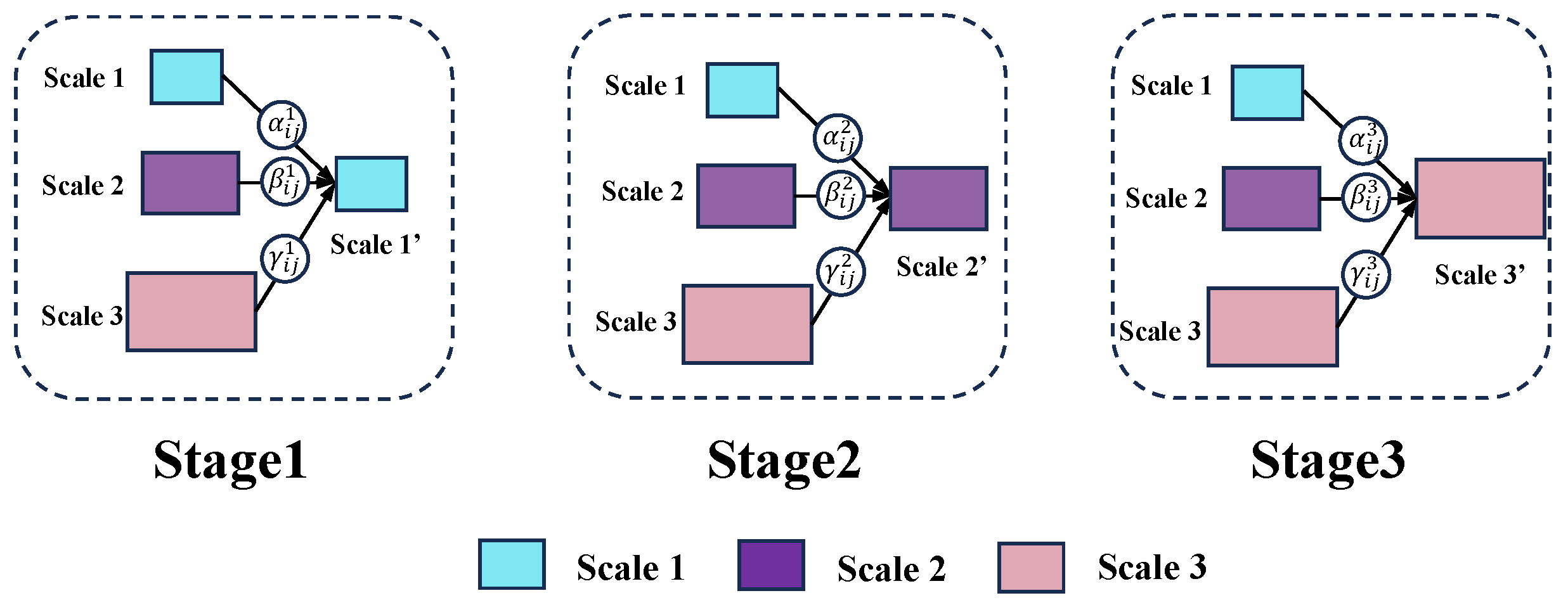
The module is achieved as follows: given each input image I i i = 1 N , we first extract a feature map at three different scales as F S n ( ( n { 1 , 2 , 3 } ) ) using the basic FPN network following previous works [21,46]. In every stage of our ASFE module, feature extraction employs shared weights across its different layers; then, to achieve the integration of feature maps at different scales, (1) we resize the feature maps in different scales to the same resolution and (2) the resized feature maps are then adaptively integrated. The ASFE network is represented in Figure 2.
(1) Resize feature maps
Given the disparities in resolution and channel count among the feature maps at three distinct stages, modifications to the up-sampling and down-sampling methodologies are correspondingly implemented for each phase. For the up-sampling procedure, a 1 × 1 convolution layer is employed to reduce the channel dimensions of feature maps to align with those observed at stage n, subsequently followed by resolution enhancement through the nearest-neighbor interpolation. In the first stage, the feature map of stage 2 is first made with 1 × 1 conv, and then the nearest-neighbor interpolation method is used to resize to 2 times the resolution of the original map. The feature map of stage 1 is first made with 1 × 1 conv and then resized to 4 times the resolution of the original map using the nearest-neighbor interpolation method. In the second stage, the feature map of stage 3 is first made with 1 × 1 conv, and then the nearest-neighbor interpolation method is used to resize it to 2 times the resolution of the original image. In the third stage, there is no up-sampling operation. The nearest-neighbor interpolation method can effectively scale feature maps. It is designed to preserve spatial information and ensure that feature maps from different scales can be aligned and fused accurately. This design assumes that up-sampling methods can provide sufficient resolution adjustment for feature fusion. The effectiveness of the ASFE relies on how well it can fuse features from different scales, which is facilitated by the alignment provided by the up-sampling method. Conversely, for the down-sampling procedure at a 1/2 scale ratio, a 3 × 3 convolution layer with a stride of 2 is utilized to diminish the channel count whilst augmenting the resolution. In scenarios involving a scale ratio of 1/4, an additional step incorporating a 2-stride max pooling layer precedes the application of a 2-stride convolution, further facilitating the adjustment process.
(2) Integrate feature map adaptively
To account for the varying importance of features at different scales, we employ a weight-based summation method to integrate these features. The weights are adaptively adjusted and learned through the ASFE network. We use F i j S l S n to denote the feature vector at the position ( i , j ) on the feature maps resized from stage l to stage n. We propose to fuse the features at the corresponding stage n as follows:
F i j S n = α i j n · F i j S 1 S n + β i j n · F i j S 2 S n + γ i j n · F i j S 3 S n
where F i j S n implies the ( i , j ) t h vector of the output feature maps F S n among the channels. α i j n , β i j n and γ i j n refer to the spatial importance weights for the feature maps at three different stages to stage n. These spatial importance weight coefficients are adaptively learned by the ASFE network. Note that α i j n , β i j n and γ i j n can be shared across all the feature channels. We force α i j n + β i j n + γ i j n = 1 and α i j n , β i j n , γ i j n [ 0 , 1 ] , and we define
α i j n = e λ α i j n e λ α i j n + e λ β i j n + e λ γ i j n
where α i j n , β i j n and γ i j n are defined by using the softmax function with λ α i j n , λ β i j n , and λ γ i j n as control parameters, respectively, which can be learned by the standard back-propagation (BP) [47].
With this network, the feature maps in all stages are adaptively aggregated at each scale. The ASFE learns how to spatially filter the features of other stages so that merely useful information is kept for combination. At each spatial location, the features of the different stages are fused adaptively. For example, some features may be filtered out as they carry useless information at this location and some may dominate with more useful clues. The final output feature maps { F i j S 1 , F i j S 2 , F i j S 3 } are used for the construction of reference and source feature volumes. The ASFE module facilitates an enhanced approach to feature integration, adeptly capitalizing on pertinent information and excluding extraneous data.

3.4. Uncertainty-Based Height Sampler

In the process of constructing cost volumes V from feature volumes F , the height ranges are mainly sampled at equal intervals [21]. However, the uniform sampler easily leads to the true height being missed in a large search range, especially in terrain reconstruction due to large pixels in satellite images and terrain fluctuations. To cope with this problem, we proposed a UBHS module to discretize the per-pixel predicted candidate range based on the matching uncertainty obtained in the last stage [22].
UBHS adopts an adaptive variable interval partition strategy to allocate dense height hypothesis planes near the possible ground true height value based on obtained matching uncertainty in the last stage and allocate relatively sparse height hypothesis planes away from it. Considering that we use the L 1 loss function as a regularization term and the terrain would hardly change abruptly locally, we use the Laplacian distribution but not the Gaussian distribution to allocate the position of the height hypothesis planes to achieve the strategy [48]. The non-uniform sampling includes two steps. Firstly, we sample at equal intervals to obtain [ h m i n ( x ) , . . . , h i ( x ) , . . . , h m a x ( x ) ] . The h i ( x ) represents the i t h height value in the sampling process. Secondly, we offset the h i ( x ) of the equal interval partition based on their related height probability. The probability is a degree that determines how possible it is that the height value is a ground truth, which can be obtained based on matching uncertainty in the last stage. So, this module involves two key parts: (1) matching uncertainty computation in the last stage; and (2) adaptive variable interval partition. The two parts are illustrated in detail as follows.
(1) Matching uncertainty computation
We utilize height map H s 1 and probability volume P s 1 predicted in the previous stage to calculate the pixel-wise matching uncertainty σ ^ ( x ) , and x denotes the image pixel. We calculate the pixel-wise matching uncertainty σ ^ ( x ) based on the variance and the corresponding probability. Specifically, we utilize the pixel-wise matching uncertainty σ ^ ( x ) and the estimated height h ^ s 1 ( x ) in stage 1 to calculate the upper and lower boundaries of the pixel-wise height range in stage 2. It is defined as Equation (3).
σ ^ ( x ) = j H p j s 1 ( x ) · h j s 1 ( x ) h ^ s 1 ( x ) 2
where p j s 1 ( x ) represents the probability of the j t h height hypothesis in stage 1. The pixel-wise height boundaries h m i n s 2 ( x ) and h m a x s 2 ( x ) are defined as Equation (4).
h m i n s 2 ( x ) = h ^ s 1 ( x ) σ ^ ( x ) , h m a x s 2 ( x ) = h ^ s 1 ( x ) + σ ^ ( x )
(2) Adaptive variable interval partition
To achieve adaptive variable interval partition, we first sample the height range at equal intervals. Then, an offset factor is computed for each interval to achieve an adaptive partition strategy. The equal intervals in the current stage h e q u a l s 2 ( x ) are defined as Equation (5).
h e q u a l s 2 ( x ) = h m a x s 2 ( x ) h m i n s 2 ( x ) H n u m s 2
where H n u m s 2 represents the number of height hypothesis planes of the current stage. The pixel-wise height hypothesis planes of stage 2 can be represented as Equation (6).
H s 2 ( x ) = [ h m i n s 2 ( x ) , . . . , h i s 2 ( x ) , . . . , h m a x s 2 ( x ) ]
where h i s 2 ( x ) denotes the i t h height hypothesis planes of stage 2.
The offset factor is defined based on Laplacian distribution. The Laplacian probability density function is f ( x | μ , b ) = 1 2 b e | x μ | b [48]. To maintain the consistency of formula form and conform to the distribution pattern, we set the offset factor as Equation (7)
offset factor = K · e ( | h i s 2 ( x ) h ^ s 1 ( x ) | δ ^ ( x ) )
where K refers to the scale factor, h i s 2 ( x ) denotes the i t h height hypothesis planes of stage 2 through equal interval partition, and h ^ s 1 ( x ) represents the estimated height of stage 1. Under this circumstance, we set K = 1 and use the softmax function to normalize the offset factor. This operation ensures the invariance of the number of height hypothesis planes in the current stage. The calculation process is formulated as Equation (8):
offset factor = s o f t m a x ( e ( | h i s 2 ( x ) h ^ s 1 ( x ) | δ ^ ( x ) ) )
Then, we leverage h i s 2 ( x ) , equal interval h e q u a l s 2 ( x ) and offset factor to calculate the new and adaptive height hypothesis planes of the current stage. This can be calculated as Equation (9).
h i s 2 ( x ) = h i s 2 ( x ) + h e q u a l s 2 ( x ) · offset factor
where h i s 2 ( x ) represents the i t h plane of hypothesis planes of the pixel-wise height range. Following the strategy of Laplacian-offset interval partition, we employ a specific offset factor for each pixel to achieve an uncertainty-based height sampler.
Within this module, it is posited that the utilization of the L 1 loss function serves as a regularization mechanism throughout the training phase. Coupled with the premise that terrain alterations exhibit minimal abruptness on a local scale, the Laplacian distribution offset factor is strategically employed to redistribute the height hypothesis planes. This computational approach is designed to enable a pixel-wise and adaptive variable interval partition strategy. By leveraging the UBHS, we advance the adoption of a more refined partition methodology, enhancing the overall efficacy of the model.

3.5. Terrain-Prior-Guided Feature Fusion

In the domain of Earth surface height estimation, the slope characteristic discernible within satellite imagery emerges as a pivotal attribute. The inherent undulations of the Earth’s surface engender variations in elevation, a dynamic readily captured through the analysis of slope feature maps [28]. Accordingly, our methodology endeavors to firstly (1) extract these slope features, and (2) subsequently fuse them to inform and refine the reconstruction process.
(1) Slope feature extraction
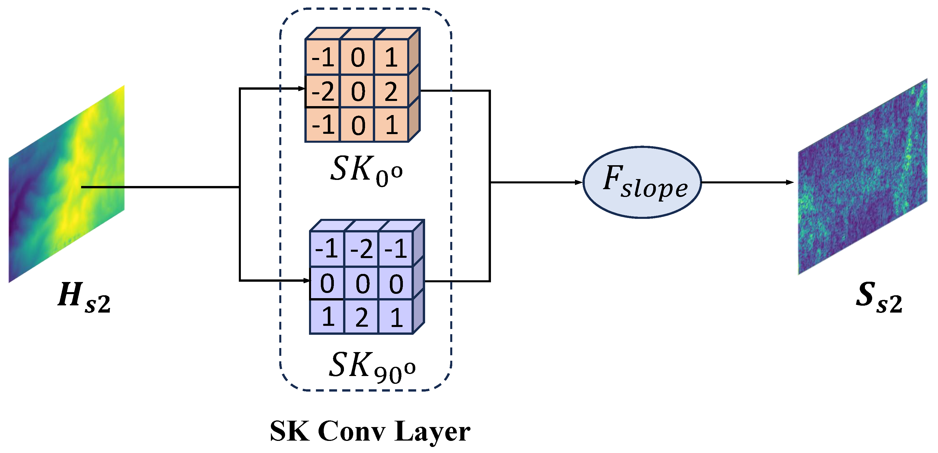
Among the pantheon of classical algorithms for linear information retrieval, the Sobel operator stands out for its efficacy, a trait that extends to the extraction of slope features [49]. To adequately harness the slope characteristic, we transform the traditional Sobel operator into two distinct directional Sobel Kernels (SK) to extract the slope features. These kernels are learnable to capture the nuanced information of the surface undulations dynamically, as illustrated in Figure 3.
As shown in Figure 3, the Sobel operator is composed of a pair of standard 3 × 3 kernels (0°–90° Sobel kernels), optimized to yield maximal responses at gradient orientations of 0° and 90° corresponding to the horizontal and vertical axes, respectively [50]. For example, the application of 0°–90° Sobel kernels within a specified grid R is articulated as Equation (10).
S 0 ° = { 1 , 0 , 1 , 2 , 0 , 2 , 1 , 0 , 1 } , S 90 ° = { 1 , 2 , 1 , 0 , 0 , 0 , 1 , 2 , 1 }
where S 0 ° denotes the 0° Sobel kernels, and S 90 ° denotes the 90° Sobel kernels. The structural representation of these 0°–90° Sobel kernels is delineated in Figure 3, offering a visual comprehension of their configuration and operational dynamics.
Utilizing the 0°–90° Sobel kernels, we adeptly ascertain the terrain’s slope. Subsequently, for the elevation map denoted by H , the slope is computed in a manner that permits differentiation, as outlined in the scholarly work of [28]. This computational methodology is succinctly encapsulated in Equation (11).
d x = [ ( h i 1 , j + 1 + 2 h i , j + 1 + h i + 1 , j + 1 ) ( h i 1 , j 1 + 2 h i , j 1 + h i + 1 , j 1 ) ] / ( 8 s ) ,
d y = [ ( h i + 1 , j 1 + 2 h i + 1 , j + h i + 1 , j + 1 ) ( h i 1 , j 1 + 2 h i 1 , j + h i 1 , j + 1 ) ] / ( 8 s ) ,
slope i j = a r c t a n d x 2 + d y 2 ,
where h i , j signifies the elevation at pixel ( i , j ) , s represents the resolution of the height map, and slope i j denotes the slope at pixel ( i , j ) . To address the challenge of elevation diversity, we introduce a Slope-Net designed to derive a comprehensive slope feature map F s l o p e , capable of encapsulating the inclinations across diverse terrain types [28]. Following this extraction, a dual encoder–decoder architecture is employed to integrate slope data into reference feature volumes F , a process meticulously detailed in the next part [51].
(2) Slope feature fusion
Drawing upon the methodologies established in image-guided depth completion [52], we introduce a bifurcated network architecture, comprising a color-dominant branch alongside a slope-dominant branch. This design is meticulously engineered to exhaustively exploit and integrate the dual modalities of color imagery and slope data. In detail, the first branch processes a color image in conjunction with a slope map, aiming to assimilate geometric information into its analysis. Conversely, the second branch processes the slope map and a pre-processed geometry-fused feature map, culminating in the production of a refined slope-geometry-fused feature map. Additionally, we innovate by integrating a series of residual structures specifically tailored to encode slope cues, complemented by a novel geometric convolutional layer devised to encapsulate 3D geometric nuances [51,53,54,55,56].
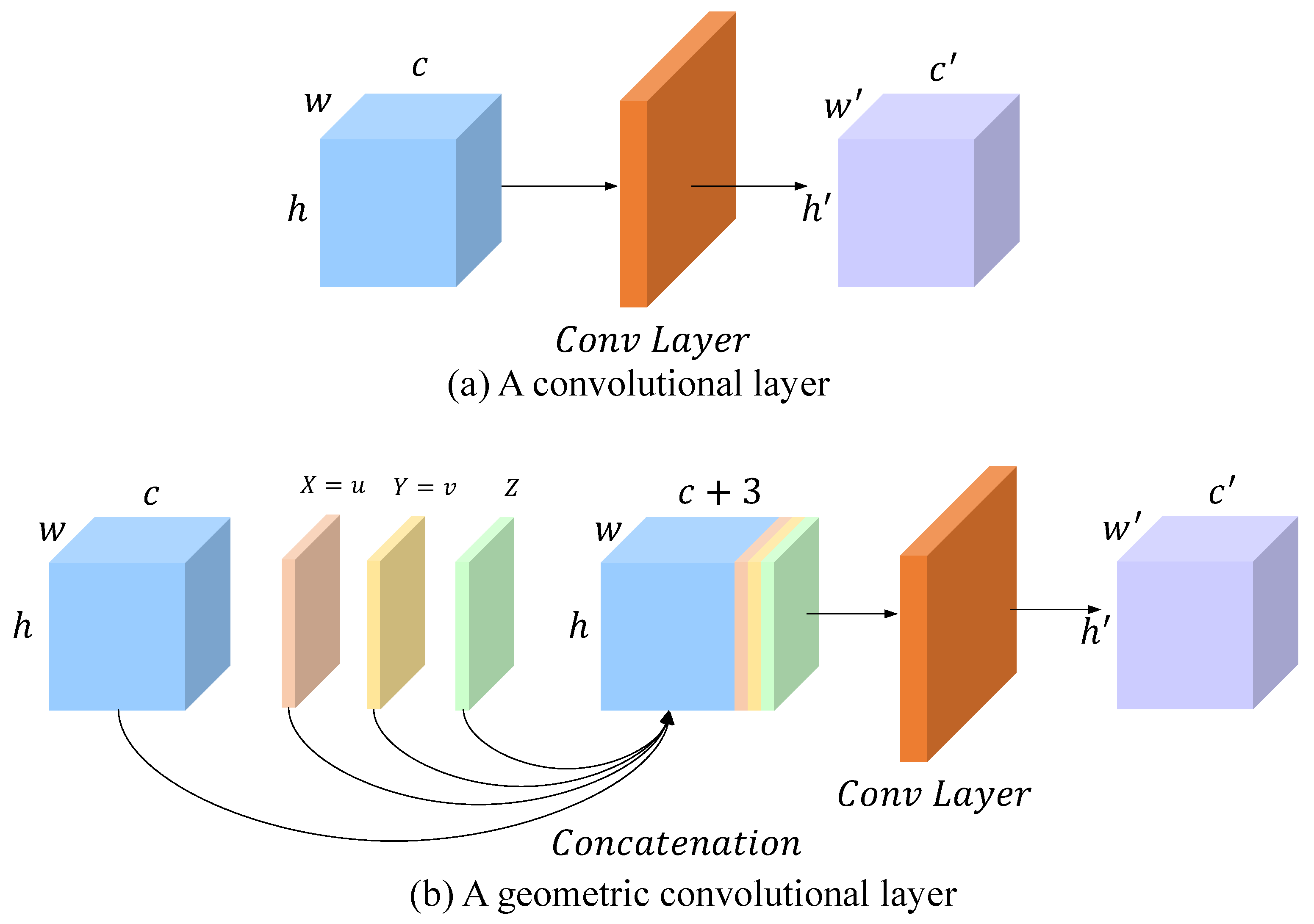
Echoing the insights of [55], the salience of 3D geometric cues in the realm of height estimation cannot be overlooked. In response, we conceptualized a geometric convolutional layer designed expressly to capture and encode 3D geometric information within its framework. The innovative design of this geometric convolutional layer is delineated in Figure 4, where it enhances the traditional convolutional layer by integrating a 3D position map with its input. This positioning map ( X , Y , Z ) employs a positional encoding scheme predicated on UV coordinates, with the encoding methodology articulated through Equation (12).
X = u , Y = v , Z = z
where ( u , v ) represents the coordinates of a pixel, and we innovate by substituting each convolutional layer within the ResBlocks with our geometric convolutional layer [53]. Through this modification, 3D geometric information is more effectively integrated into the feature representation within the dual encoder–decoder architecture.
The architecture of the dual encoder–decoder network is illustrated in Figure 5. This network is meticulously engineered to fully leverage and integrate the distinct modalities of color-dominant and slope-dominant information via their respective branches, thus optimizing the efficacy of modality fusion. The color-dominant branch is specifically designed to harness the structural information present in the color image. Within this branch, an encoder–decoder configuration is employed, featuring symmetric skip connections to facilitate information flow [57]. The encoder is composed of one geometric convolutional layer and six foundational residual blocks, i.e., ResBlocks [53], whereas the decoder is equipped with three deconvolution layers and a final convolution layer, with each convolutional operation succeeded by a batch normalization (BN) layer and a ReLU activation function [58,59].
The slope-dominant branch is strategically designed to exploit the wealth of slope information contained within the slope feature map. To facilitate a comprehensive feature integration, we introduce an innovative decoder–encoder fusion approach, enabling the incorporation of attributes from the color-dominant branch into the slope-focused branch. This integration is executed through the concatenation of decoder outputs from the color-dominant branch with their corresponding encoder inputs in the slope-dominant branch. The dual encoder–decoder network yields a feature map influenced by the slope priors of the reference image I 1 . The derivation of the slope-guided feature map for the reference image I 1 in the subsequent n + 1 stage is delineated in Equation (13).
O ( x ) = B ^ ( [ S 1 n , B ( [ I 1 n + 1 , S 1 n ] ) ] ) ,
F ^ 1 n + 1 ( x ) = F u s i o n { F 1 n + 1 ( x ) O ( x ) } ,
where x signifies the pixel within the image, S 1 n represents the slope map derived from the elevation map, and the symbols [ , ] and ⊕ are utilized to denote the operations of concatenation and element-wise addition, respectively. Within this equation, B symbolizes the color-dominant branch, while B ^ identifies the terrain-dominant branch. O ( x ) encapsulates the fusion feature map output by the dual encoder–decoder network. Furthermore, F 1 n + 1 ( x ) denotes the feature map originating from the basic FPN network, whereas F ^ 1 n + 1 ( x ) represents the feature map that is both guided by slope features and fused by geometric clues. The key to terrain reconstruction is feature matching. The slope information represents the relief characteristics of the terrain. The use of residual blocks can help alleviate the problem of disappearing gradients, and help the network better learn the input slope features and geometric structure features. Slope features and geometric structure features provide more features for feature matching, which means that more effective information is available in the feature matching step, so it will be conducive to improving the accuracy of terrain reconstruction.
In conclusion, the two-branch encoder–decoder architecture with residual blocks can help us estimate the height more accurately. Diverging from the path tread by preceding studies, which often necessitate complex external dependencies, our approach innovates by directly integrating terrain priors gleaned from previous depth assessments into the feature volumes, thus enhancing the fusion process.

3.6. Loss Function

We employ the mean absolute difference between the ground truth height map and the estimated height map as the training loss of the network [21]. The cascade cost volume with N stages leads to N 1 temporary output results and a final prediction. We adopt the supervision to all the outputs of all the stages and the total loss function is defined as Equation (14):
L k = p p v a l i d | | d ( p ) d ^ k ( p ) | | 1 L o s s 1 ,
L o s s t o t a l = k = 1 N λ k · L k ,
where L k represents the loss at the k t h stage and λ k refers to its corresponding loss weight. p v a l i d represents the set of valid ground truth pixels, d ( p ) denotes the ground truth depth value of pixel p, d ^ k ( p ) refers to the k t h stage depth estimation, and | | | | 1 represents the L 1 loss function. The number of stages, N, is set to 3. The depth loss weights λ k for three stages are set to [ 0.5 , 1.0 , 2.0 ] .

4. Experiment

4.1. The Dataset

In the realm of satellite MVS using deep learning, we are presently confronted with a substantial scarcity of training datasets. To our understanding, the relevant datasets available for this purpose are WHU-TLC [5] and UCS3D [26]. However, the US3D dataset aims to serve the joint task of semantic segmentation and 3D reconstruction, where the scene variations between the stereo image pairs are not suitable for high-accuracy MVS reconstruction [24], so we do not use this dataset in our pipeline. Therefore, we use the WHU-TLC dataset in our experiments.
WHU-TLC dataset: The WHU-TLC dataset is a large-scale MVS satellite image dataset built to advance the development of satellite dense matching and 3D reconstruction [5]. There are 173 scenes in the dataset, including 127 for training and 46 for testing. The triple-view images were acquired from the TLC mounted on the ZY3-02 satellite [24], and have been cropped to patches of 5120 × 5120 pixels. The ground resolutions of nadir, 22° forward, and backward view are 2.1 m, 2.7 m, and 2.7 m, respectively. The RPC models have been aligned with the provided DSMs, and the DSMs are stored as regular grids with a resolution of 5 m under the WGS-84 geodetic and the Universal Transverse Mercator (UTM) projection coordinate systems.

4.2. Evaluation Metrics

In our study, we employ the metrics outlined by Gao et al. [5] to assess the quality of the depth maps derived across the WHU-TLC dataset. These metrics are crucial for evaluating both the accuracy and effectiveness of our depth estimation process. We define these metrics as follows:
(1) MAE (mean absolute error): MAE measures the average L 1 distance between the estimated DSM and the ground truth across all valid grid cells. The mathematical expression for MAE is presented in Equation (15):
M A E = ( i , j ) D D ˜ h i j h ˜ i j ( i , j ) D D ˜ I v e r ( i , j ) D D ˜
Here, D and D ˜ represent the sets of valid grid cells in the estimated and true DSMs, respectively; h i j and h ˜ i j denote the height values at grid cell ( i , j ) for the estimation and truth, respectively; and Iver ( A ) is the Iverson bracket, which equals 1 if A is true, and 0 otherwise.
(2) RMSE (root mean square error): RMSE quantifies the standard deviation of the residuals between the estimated values and the actual values within the DSM. This metric is defined as in Equation (16):
R M S E = ( i , j ) D D ˜ ( h i j h ˜ i j ) 2 ( i , j ) D D ˜ Iver ( ( i , j ) D D ˜ )
(3) <2.5 m (accuracy within 2.5 m threshold): This metric calculates the percentage of grid cells where the L 1 distance error is less than 2.5 m. It is mathematically defined in Equation (17):
< 2.5 m = ( i , j ) D D ˜ ( | h i j h ˜ i j | < 2.5 ) ( i , j ) D D ˜ Iver ( ( i , j ) D D ˜ )
(4) <7.5 m (accuracy within 7.5 m threshold): Similarly, this metric assesses the percentage of grid cells where the L 1 distance error is less than 7.5 m, as shown in Equation (18):
< 7.5 m = ( i , j ) D D ˜ ( | h i j h ˜ i j | < 7.5 ) ( i , j ) D D ˜ Iver ( ( i , j ) D D ˜ )
(5) Comp (completeness): This metric determines the percentage of grid cells that contain valid height values in the final DSM.
These metrics are integral to our evaluation, allowing for a comprehensive analysis of the model’s performance.

4.3. Implemented Details

In this experiment, following SatMVS(CasMVSNet) [24], we trained our SA-SatMVS on the WHU-TLC-v2 dataset and evaluated our pre-trained model on the WHU-TLC test dataset.
Training. We have completed our proposed SA-SatMVS using PyTorch and trained this model on the WHU-TLC-v2 dataset. During the training process, SA-SatMVS was trained on the WHU-TLC-v2 dataset using 2x NVIDIA RTX 4090 GPUs, each with 24 GB of memory. The training hyperparameters were configured as follows: batch size of 4, and RMSProp was selected as the optimizer with an α value of 0.9. The model was trained for 30 epochs, beginning with a learning rate of 0.001, which was halved after the 10th epoch. We employed a three-stage hierarchical matching approach to infer height maps from coarse-to-fine scales. For the WHU-TLC-v2 images, the number of input images, represented as n, was fixed at 3, comprising 1 reference image and 2 source images. The numbers of hypothetical height planes of three stages were set to [64, 32, 8], and their corresponding intervals were set to [ H R h H R l 64 , 5 m, 2.5 m], respectively, where H R h and H R l separately represented the high bound and the low bound of the height range of the WHU-TLC-v2 image.
Testing. We tested the best model obtained during the training process on the WHU-TLC test dataset, cropping the images of 5120 × 5120 pixels into the images of 768 × 384 pixels and using 3 adjacent images of 768 × 384 pixels as the input, respectively. The hypothetical height planes for testing were set to [64, 32, 8] and their corresponding intervals were set to [ H R h H R l 64 , 5 m, 2.5 m]. Finally, we applied the aforementioned evaluation metrics to evaluate the quality of the predicted height maps. In the process of DSM production, we adopted the SatMVS pipeline to infer height maps and generate corresponding point clouds. The point clouds generated by these height maps were then incorporated to obtain the digital surface models (DSMs). These DSMs served as visual results to evaluate the performance of our model.

4.4. Results

4.4.1. Analysis on Height Map

(1) Quantitative analysis
Height maps constitute essential intermediary outputs that are integral to the majority of MVSNet methodologies, serving as foundational elements from which digital surface model (DSM) results are subsequently extrapolated. In this context, an in-depth analysis of height maps produced by diverse implementations of MVSNet methodologies is undertaken to foster a nuanced understanding. Evaluation metrics paralleling those utilized in DSM generation are applied, albeit with grid cell values being substituted by height measurements. The evaluation metrics are MAE , < 2.5   m   ( % ) , < 7.5   m   ( % ) . The RMSE metric and the completeness metric are specific to the DSM results. The results are shown in Table 1.
As delineated in Table 1, we can observe that the superiority of our proposed model in reconstructing the WHU-TLC-v2 dataset is manifest, especially for the mean absolute error (MAE) and δ < 2.5 m performance metrics. The MAE metrics of SatMVS(RED-Net), SatMVS(CasMVSNet), and SatMVS(UCS-Net) are 1.836, 1.979, and 1.875, respectively. Notably, our framework achieves significant reductions in the MAE metric by 0.132, 0.275, and 0.171 in comparison to SatMVS (RED-Net), SatMVS (CasMVSNet), and SatMVS (UCS-Net), respectively. Our model achieves the best MAE metric of 1.704 regarding quantitative results on the height maps.
Furthermore, the δ < 2.5 m metrics of SatMVS(RED-Net), SatMVS(CasMVSNet), and SatMVS(UCS-Net) are 82.06, 81.89, and 81.96, respectively. Relative to these approaches, our methodology registers enhancements of 1.96, 2.13, and 2.06 in the δ < 2.5 m metric, respectively. We gain the state-of-the-art δ < 2.5 m metric of 84.02. Concurrently, our method procures results in the δ < 7.5 m metric that are on par with those of existing models.
The observed advancements are primarily ascribed to the strategic integration of slope feature information and cross-scale information synthesis within our approach, enabling the model to exploit terrain characteristics to the fullest and substantially refine the accuracy of height map estimations.
(2) Qualitative analysis
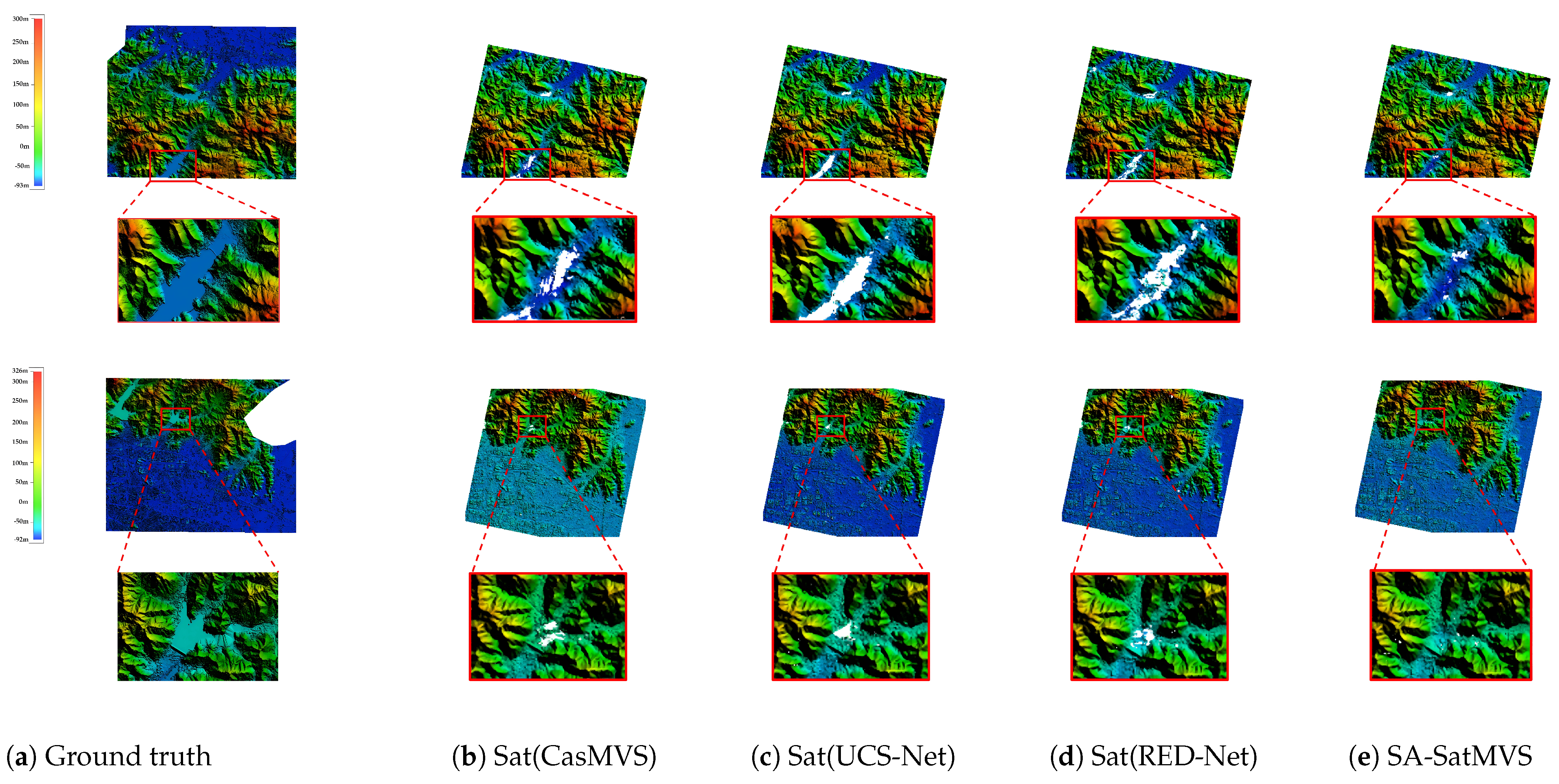
We also provide visual representations of the outcomes derived from various models, as shown in Figure 6. We can observe that our methodology manifests a notable reduction in void areas, thereby facilitating more accurate height map estimations. These void regions, indicative of matching failures, emerge in scenarios fraught with complexities such as occlusions, cloud cover, shadows, and textureless water surfaces. Such proficiency in our approach can be attributed to its comprehensive strategy that seamlessly integrates multi-scale information and incorporates terrain slope attributes into the analytic framework. This synergistic integration is instrumental in markedly diminishing the incidence of unmatched regions, underscoring the robustness and precision of our proposed model.

4.4.2. Analysis on DSM

(1) Quantitative analysis
In former deep learning-based MVS methods, homography warping was utilized to align images from different viewpoints to a reference view through a set of hypothetical fronto-parallel depth planes of the reference camera [20,21,22]. However, in the field of large-scale and precise 3D reconstruction of the Earth’s surface, we use RPC warping to align multi-view satellite images with the reference image to improve accuracy and completeness. To showcase the effectiveness of our proposed model, we conducted comparisons with the traditional MVS method [13] and deep learning-based MVS methods [5]. Specifically, we evaluated our method alongside three deep learning MVS methods, namely RED-Net, CasMVSNet, and UCS-Net, which were also adapted to SatMVS and denoted as SatMVS(RED-Net), SatMVS(CasMVSNet), and SatMVS(UCS-Net). Table 2 presents the quantitative results on the WHU-TLC dataset (test set).
As depicted in Table 2, our method achieves the highest scores across the most effectiveness metrics compared to other methods, which is deemed acceptable. In the field of DSM results, the MAE metric of the traditional method Adapted COLMAP is 2.227. The MAE metrics of deep learning-based methods such as RED-Net, CasMVSNet, and UCS-Net are 2.171, 2.031, and 2.039, respectively. Notably, our method demonstrates notable improvements over the Adapted COLMAP and RED-Net, CasMVSNet, and UCS-Net, with reductions in the MAE metric by 0.348, 0.292, 0.152, and 0.16, respectively. The MAE metrics of the adapted SatMVS methods such as SatMVS(RED-Net), SatMVS(CasMVSNet), and SatMVS(UCS-Net) are 1.945, 2.020, and 2.026. Our method also outperforms the MAE metric, with superiority values of 0.066, 0.141, and 0.147, respectively. Our model achieves the best MAE metric of 1.879.
Moreover, the RMSE metric of Adapted COLMAP is 5.291. And, the RMSE metrics of RED-Net, CasMVSNet, and UCS-Net are 4.514, 4.351, and 4.084, respectively. Our proposed framework exhibits decreases in the RMSE metric by 1.506 compared to the traditional approach and by 0.729, 0.566, and 0.299 compared to the aforementioned deep learning-based methods. The RMSE metrics of SatMVS (RED-Net), SatMVS (CasMVSNet), and SatMVS (UCS-Net) are 4.070, 3.841, and 3.921. Our method also outperforms the RMSE metric, with superiority values of 0.285, 0.056, and 0.136, respectively. Our framework gains the state-of-the-art RMSE metric of 3.785. These improvements can be attributed to our use of the UBHS module, which applies the information in the last stage to guide the height sampling process, thus achieving more accurate predictions of height or grid cell values.
Furthermore, the δ < 2.5 m metric of the traditional method Adapted COLMAP is 73.35. The δ < 2.5 m metrics of RED-Net, CasMVSNet, and UCS-Net are 74.13, 77.39, and 76.40. And, the δ < 2.5 m metrics of SatMVS (RED-Net), SatMVS (CasMVSNet), and SatMVS (UCS-Net) are 77.93, 76.79, and 77.01. Our method achieves significant advancements with the δ < 2.5 m metric of 79.02. Apart from this, the δ < 7.5 m metric of the Adapted COLMAP is 96.00. The δ < 7.5 m metrics of RED-Net, CasMVSNet, and UCS-Net are 95.91, 96.53, and 96.66. And, the δ < 7.5 m metrics of SatMVS (RED-Net), SatMVS (CasMVSNet), and SatMVS (UCS-Net) are 96.59, 96.73, and 96.54. Our method achieved significant advancements with the δ < 7.5 m metric of 96.62. The δ < 2.5 m metric and δ < 7.5 m metric are crucial for accurate DSM construction and hold substantial value for the Earth’s surface reconstruction.
Additionally, the completeness metric of the traditional method Adapted COLMAP is 79.10. The completeness metrics of RED-Net, CasMVSNet, and UCS-Net are 81.82, 82.33, and 82.08. The completeness metrics of SatMVS (RED-Net), SatMVS (CasMVSNet), and SatMVS (UCS-Net) are 82.29, 81.54, and 82.21. Our framework demonstrates impressive results in terms of completeness, with a completeness metric of 82.37, underscoring the significant potential of our method in satellite image reconstruction.
These observations indicate the state-of-the-art performance of our approach, which can be attributed to the incorporation of slope feature information, enabling the model to capitalize on terrain advantages and enhance the quality of height map estimation.
(2) Qualitative analysis
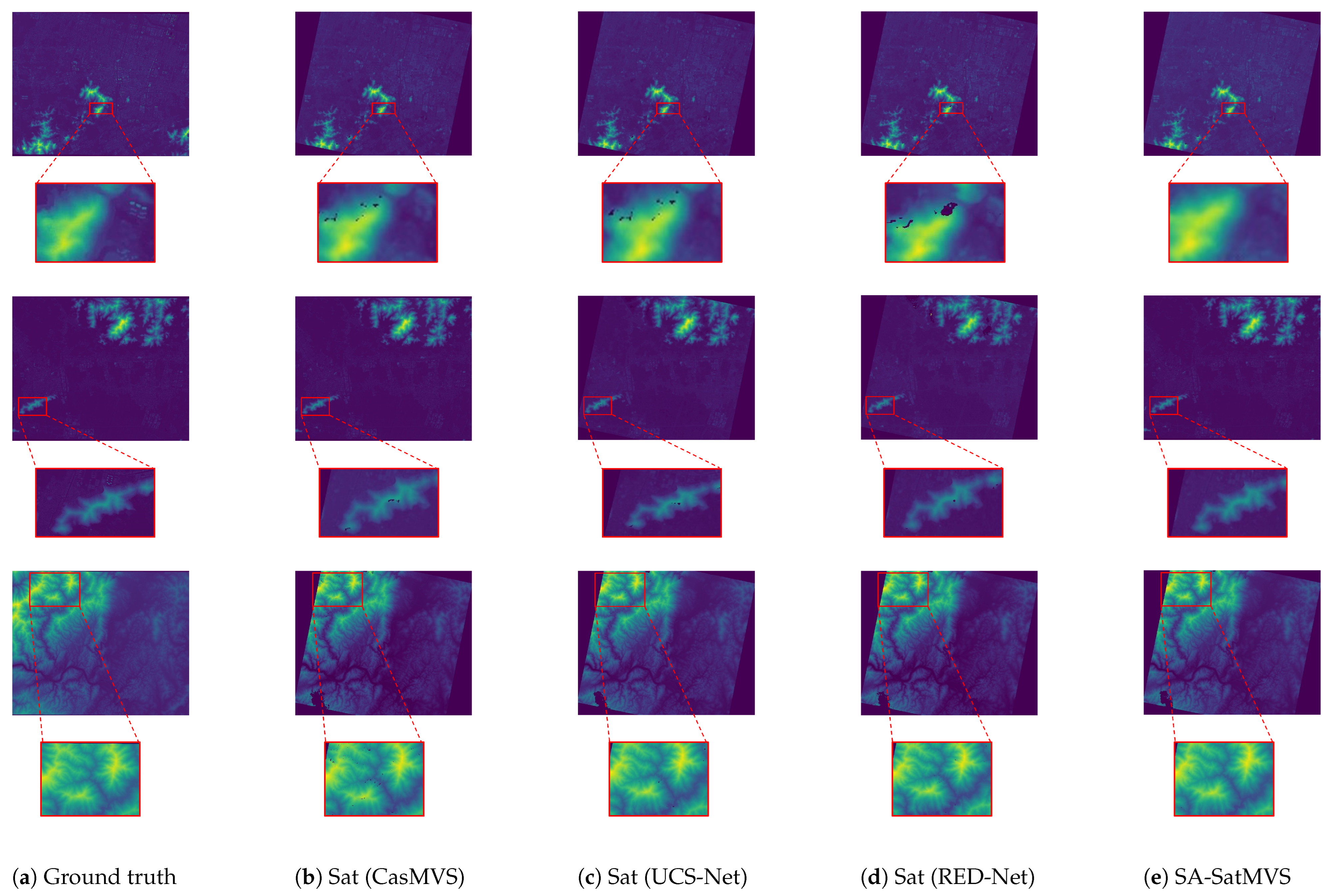
We also present several DSM visualization results to validate the effectiveness of our proposed model in Figure 7, where invalid matches are highlighted in white. The results in Figure 7 indicate that our proposed model exhibits minimal apparent invalid matches compared to SatMVS (RED-Net), SatMVS (CasMVSNet), and SatMVS (UCS-Net), suggesting superior accuracy and a high level of completeness. This performance can be attributed to several factors. Firstly, our ASFE module enables the filtration of irrelevant information by assigning higher weights to useful data. Secondly, the UBHF module facilitates pixel-wise height interval partition, aligning more closely with the data distribution of the model and thereby enhancing matching precision. Additionally, the incorporation of terrain features via the TPGF module ensures more comprehensive and complete matched features, consequently leading to higher matching completeness. Furthermore, in mountainous areas, the introduction of slope characteristics and the encoding of image pixel positions enable our model to capture more terrain features and positional information of matching points. These factors contribute to the enhanced effectiveness of the 3D reconstruction of the Earth’s surface.

4.5. Ablation Study

4.5.1. Ablation Study on the Novel Modules

In this section, we set our proposed approach as a baseline. We then conducted an ablation study by excluding each module sequentially to understand and analyze the contributions of the modules of our architecture. The experimental results are shown in Table 3.
Effectiveness of ASFE. As shown in Table 3, we observe worse performance in all metrics when ASFE is excluded from SA-SatMVS. Specifically, the MAE improves from 1.879 to 1.945, the RMSE improves from 3.785 to 3.833, the percentage of δ < 2.5 m decreases from 79.02 to 78.71, the percentage of δ < 7.5 m decreases from 96.62 to 96.31, and the completeness decreases from 82.37 to 82.31. These findings highlight the adaptability of our ASFE, which effectively fuses features across different scales. This operation enables the extraction of more valuable information from input images while filtering out contradictory data, ultimately enhancing the reconstruction quality.
Effectiveness of UBHS. As shown in Table 3, we observe worse performance in all metrics when UBHS is excluded from SA-SatMVS. Specifically, the MAE improves from 1.879 to 1.968, and the RMSE improves from 3.785 to 3.841. These two enhancements can be attributed to the utilization of Laplacian distribution-based offset calculation in our proposed UBHS. In the case of large-scale scenes, the two-stage UBHS module can effectively explore accurate height values within a reduced pixel-wise height range, contributing to a higher level of precision in the height map. Furthermore, the percentage of δ < 2.5 m decreases from 79.02 to 78.47, the percentage of δ < 7.5 m decreases from 96.62 to 96.45, and the completeness decreases from 82.37 to 82.29. These can be attributed to the fact that our proposed UBHS can also effectively leverage the pixel-wise elevation information provided by the previous stage to mitigate the impact of terrain undulations. The UBHS module makes full use of the height-probability information provided by the previous stage. All the consequences corroborate the effectiveness of our proposed UBHS module.
Effectiveness of TPGF. As shown in Table 3, we observe a worse performance in all metrics when TPGF is excluded from SA-SatMVS. Specifically, the MAE metric increased from 1.879 to 1.973, and the RMSE metric increased from 3.785 to 3.863, correspondingly. The above results distinctly show the excellence of the guidance of the terrain feature. The reason is that the geometry awareness network (TPGF) can fully explore the inherent geometric structure information without introducing external dependencies. The decrease in the percentage of δ < 2.5 m (78.34 vs. 79.02) and δ < 7.5 m (96.37 vs. 96.62) also proves the utility of the module. Incorporating slope features can notably alleviate issues related to large terrain undulations and height variations. The thorough exploration and integration of slope features and geometric structural characteristics also enhance the completeness of reconstruction results. The TPGF module can provide more effective information for feature matching. All the above findings illustrate the significance of fully exploiting terrain features.

4.5.2. Ablation Study on the Softmax Function

The softmax function in Equation (8) can also be replaced by other ones, such as the linear normalized function. We also performed a comparison by applying the linear normalized functions and the exponential softmax function (adopted in our approach). The results are shown in Table 4 and Table 5. We can observe from Table 4 that the model with the exponential softmax function (Equation (8)) achieves better in the MAE metric (1.704 vs. 1.786), the δ < 2.5 m metric (84.02 vs. 83.59), and the δ < 7.5 m metric (96.77 vs. 96.61). In Table 5, we can observe that the MAE metric of the DSM results increased from 1.879 to 1.933, the RMSE metric increased from 3.785 to 3.894, and the completeness decreased from 82.37 to 82.16 while applying the exponential softmax function. These results indicate the effectiveness of our applied exponential softmax function.

5. Limitations and Discussion

Although our model achieves a better or comparable performance than most the state-of-the-art methods, it has several limitations.
  • In the realm of satellite multi-view stereo matching, the fusion of multi-modal data presents a notable challenge, underscoring a persistent issue in achieving optimal terrain reconstruction. Our approach adopts an encoder–decoder framework, enhanced with residual blocks, for the amalgamation of data across various modalities. Furthermore, we remain committed to investigating alternative strategies for data fusion, aiming to refine and expand the efficacy of our methodology in addressing the nuanced demands of satellite multi-view stereo matching.
  • The acquisition of high-quality, high-resolution datasets plays a crucial role in facilitating more precise terrain reconstruction outcomes. Our methodology endeavors to mitigate these limitations by dynamically integrating features across various scales, effectively harnessing both local and global feature sets to enhance the reconstruction process. Moving forward, we anticipate the development of additional methodologies and strategies aiming to overcome these challenges, further advancing the field of terrain reconstruction.

6. Conclusions

In this paper, we propose a novel multi-stage coarse-to-fine SA-SatMVS framework for high-quality large-scale Earth surface reconstruction. Our ASFE module utilizes the reference image and source images to adaptively extract different scales of features, which can take advantage of more useful information and filter contradictory information. This module can search for the optimal fusion of features across three different scales with minimal computational cost. Furthermore, the UBHS module can reallocate the pixel-wise height interval to obtain more accurate height values by leveraging the Laplacian distribution for adaptive interval partition. Moreover, the TPGF module can make full use of the terrain features to guide the process of height estimation. The results demonstrate that our proposed approach achieves a state-of-the-art performance and reveals a competitive generalization ability compared to all the listed methods. We hope that our work can contribute to the development of the Earth’s surface reconstruction from MVS satellite images. In light of the extant constraints characteristic of multi-view stereo research, our future work will concentrate on refining the robustness and accuracy of our method. Acknowledging the critical influence of illumination variations on the performance of SA-SatMVS, we recognize the imperative need to develop advanced algorithms capable of adjusting to diverse natural conditions. This focus not only addresses a significant limitation but also paves the way for enhancing the applicability and reliability of multi-view stereo techniques across a broader spectrum of real-world scenarios.

Author Contributions

Conceptualization, X.C. and S.Z.; methodology, X.C.; software, X.C.; validation, X.C.; investigation, X.C.; data curation, X.C.; writing original draft preparation, X.C.; writing review and editing, C.L., Z.W. and W.D.; project administration, C.L. All authors have read and agreed to the published version of the manuscript.

Funding

This research was supported by the National Natural Science Foundation of China (No.62331027).

Data Availability Statement

The WHU-TLC dataset and WHU-TLC-v2 dataset presented in the study are openly available at http://gpcv.whu.edu.cn/data/whu_tlc.html accessed on 1 July 2023.

Conflicts of Interest

The authors declare no conflicts of interest.

References

  1. Kril, T.; Shekhunova, S. Terrain elevation changes by radar satellite images interpretation as a component of geo-environmental monitoring. In Proceedings of the Monitoring 2019. European Association of Geoscientists & Engineers, The Hague, The Netherlands, 8–12 September 2019; Volume 2019, pp. 1–5. [Google Scholar]
  2. Maksimovich, K.Y.; Garafutdinova, L. GIS-Based Terrain Morphometric Analysis for Environmental Monitoring Tasks. J. Agric. Environ. 2022, 21. [Google Scholar]
  3. Storch, M.; de Lange, N.; Jarmer, T.; Waske, B. Detecting Historical Terrain Anomalies with UAV-LiDAR Data Using Spline-Approximation and Support Vector Machines. IEEE J. Sel. Top. Appl. Earth Obs. Remote Sens. 2023, 16, 3158–3173. [Google Scholar] [CrossRef]
  4. Shao, Z.; Yang, N.; Xiao, X.; Zhang, L.; Peng, Z. A multi-view dense point cloud generation algorithm based on low-altitude remote sensing images. Remote Sens. 2016, 8, 381. [Google Scholar] [CrossRef]
  5. Gao, J.; Liu, J.; Ji, S. Rational polynomial camera model warping for deep learning based satellite multi-view stereo matching. In Proceedings of the IEEE/CVF International Conference on Computer Vision 2021, Montreal, BC, Canada, 11–17 October 2021; pp. 6148–6157. [Google Scholar]
  6. Zhou, L.; Zhang, Z.; Jiang, H.; Sun, H.; Bao, H.; Zhang, G. DP-MVS: Detail preserving multi-view surface reconstruction of large-scale scenes. Remote Sens. 2021, 13, 4569. [Google Scholar] [CrossRef]
  7. Gonçalves, G.; Gonçalves, D.; Gómez-Gutiérrez, Á.; Andriolo, U.; Pérez-Alvárez, J.A. 3D reconstruction of coastal cliffs from fixed-wing and multi-rotor uas: Impact of sfm-mvs processing parameters, image redundancy and acquisition geometry. Remote Sens. 2021, 13, 1222. [Google Scholar] [CrossRef]
  8. Kada, M.; McKinley, L. 3D building reconstruction from LiDAR based on a cell decomposition approach. Int. Arch. Photogramm. Remote Sens. Spat. Inf. Sci. 2009, 38, W4. [Google Scholar]
  9. Li, N.; Su, B. 3D-Lidar based obstacle detection and fast map reconstruction in rough terrain. In Proceedings of the 2020 5th International Conference on Automation, Control and Robotics Engineering (CACRE), Dalian, China, 19–20 September 2020; pp. 145–151. [Google Scholar]
  10. Do, P.N.B.; Nguyen, Q.C. A review of stereo-photogrammetry method for 3-D reconstruction in computer vision. In Proceedings of the 2019 19th International Symposium on Communications and Information Technologies (ISCIT), Ho Chi Minh City, Vietnam, 25–27 September 2019; pp. 138–143. [Google Scholar]
  11. Lorensen, W.E.; Cline, H.E. Marching cubes: A high resolution 3D surface construction algorithm. In Seminal Graphics: Pioneering Efforts That Shaped the Field; Association for Computing Machinery: New York, NY, USA, 1998; pp. 347–353. [Google Scholar]
  12. Newman, T.S.; Yi, H. A survey of the marching cubes algorithm. Comput. Graph. 2006, 30, 854–879. [Google Scholar] [CrossRef]
  13. Zhang, K.; Snavely, N.; Sun, J. Leveraging vision reconstruction pipelines for satellite imagery. In Proceedings of the IEEE/CVF International Conference on Computer Vision Workshops 2019, Seoul, Republic of Korea, 27–28 October 2019. [Google Scholar]
  14. Toutin, T. Geometric processing of IKONOS Geo images with DEM. In Proceedings of the ISPRS Joint Workshop High Resolution from Space 2001, Hannover, Germany, 19–21 September 2001; pp. 19–21. [Google Scholar]
  15. Pham, N.T.; Park, S.; Park, C.S. Fast and efficient method for large-scale aerial image stitching. IEEE Access 2021, 9, 127852–127865. [Google Scholar] [CrossRef]
  16. Zarei, A.; Gonzalez, E.; Merchant, N.; Pauli, D.; Lyons, E.; Barnard, K. MegaStitch: Robust Large-scale image stitching. IEEE Trans. Geosci. Remote Sens. 2022, 60, 1–9. [Google Scholar] [CrossRef]
  17. Chen, L.; Zhao, Y.; Xu, S.; Bu, S.; Han, P.; Wan, G. Densefusion: Large-scale online dense pointcloud and dsm mapping for uavs. In Proceedings of the 2020 IEEE/RSJ International Conference on Intelligent Robots and Systems (IROS), Las Vegas, NV, USA, 25–29 October 2020; pp. 4766–4773. [Google Scholar]
  18. Qin, R.; Gruen, A.; Fraser, C. Quality assessment of image matchers for DSM generation–a comparative study based on UAV images. arXiv 2021, arXiv:2108.08369. [Google Scholar]
  19. Seitz, S.M.; Curless, B.; Diebel, J.; Scharstein, D.; Szeliski, R. A comparison and evaluation of multi-view stereo reconstruction algorithms. In Proceedings of the 2006 IEEE Computer Society Conference on Computer Vision and Pattern Recognition (CVPR’06), New York, NY, USA, 17–22 June 2006; Volume 1, pp. 519–528. [Google Scholar]
  20. Yao, Y.; Luo, Z.; Li, S.; Fang, T.; Quan, L. Mvsnet: Depth inference for unstructured multi-view stereo. In Proceedings of the European Conference on Computer Vision (ECCV) 2018, Munich, Germany, 8–14 September 2018; pp. 767–783. [Google Scholar]
  21. Gu, X.; Fan, Z.; Zhu, S.; Dai, Z.; Tan, F.; Tan, P. Cascade cost volume for high-resolution multi-view stereo and stereo matching. In Proceedings of the IEEE/CVF Conference on Computer Vision and Pattern Recognition 2020, Seattle, WA, USA, 13–19 June 2020; pp. 2495–2504. [Google Scholar]
  22. Cheng, S.; Xu, Z.; Zhu, S.; Li, Z.; Li, L.E.; Ramamoorthi, R.; Su, H. Deep stereo using adaptive thin volume representation with uncertainty awareness. In Proceedings of the IEEE/CVF Conference on Computer Vision and Pattern Recognition 2020, Seattle, WA, USA, 13–19 June 2020; pp. 2524–2534. [Google Scholar]
  23. Weilharter, R.; Fraundorfer, F. Highres-mvsnet: A fast multi-view stereo network for dense 3d reconstruction from high-resolution images. IEEE Access 2021, 9, 11306–11315. [Google Scholar] [CrossRef]
  24. Gao, J.; Liu, J.; Ji, S. A general deep learning based framework for 3D reconstruction from multi-view stereo satellite images. ISPRS J. Photogramm. Remote Sens. 2023, 195, 446–461. [Google Scholar] [CrossRef]
  25. Bosch, M.; Kurtz, Z.; Hagstrom, S.; Brown, M. A multiple view stereo benchmark for satellite imagery. In Proceedings of the 2016 IEEE Applied Imagery Pattern Recognition Workshop (AIPR), Washington, DC, USA, 18–20 October 2016; pp. 1–9. [Google Scholar]
  26. Bosch, M.; Foster, K.; Christie, G.; Wang, S.; Hager, G.D.; Brown, M. Semantic stereo for incidental satellite images. In Proceedings of the 2019 IEEE Winter Conference on Applications of Computer Vision (WACV), Waikoloa Village, HI, USA, 7–11 January 2019; pp. 1524–1532. [Google Scholar]
  27. Cheng, L.; Guo, Q.; Fei, L.; Wei, Z.; He, G.; Liu, Y. Multi-criterion methods to extract topographic feature lines from contours on different topographic gradients. Int. J. Geogr. Inf. Sci. 2022, 36, 1629–1651. [Google Scholar] [CrossRef]
  28. Zhang, Y.; Yu, W.; Zhu, D. Terrain feature-aware deep learning network for digital elevation model superresolution. ISPRS J. Photogramm. Remote Sens. 2022, 189, 143–162. [Google Scholar] [CrossRef]
  29. Chen, P.H.; Yang, H.C.; Chen, K.W.; Chen, Y.S. MVSNet++: Learning depth-based attention pyramid features for multi-view stereo. IEEE Trans. Image Process. 2020, 29, 7261–7273. [Google Scholar] [CrossRef]
  30. Mi, Z.; Di, C.; Xu, D. Generalized binary search network for highly-efficient multi-view stereo. In Proceedings of the IEEE/CVF Conference on Computer Vision and Pattern Recognition 2022, New Orleans, LA, USA, 18–24 June 2022; pp. 12991–13000. [Google Scholar]
  31. Zhang, S.; Xu, W.; Wei, Z.; Zhang, L.; Wang, Y.; Liu, J. ARAI-MVSNet: A multi-view stereo depth estimation network with adaptive depth range and depth interval. Pattern Recognit. 2023, 144, 109885. [Google Scholar] [CrossRef]
  32. Ma, X.; Wang, Z.; Li, H.; Zhang, P.; Ouyang, W.; Fan, X. Accurate monocular 3d object detection via color-embedded 3d reconstruction for autonomous driving. In Proceedings of the IEEE/CVF International Conference on Computer Vision 2019, Seoul, Republic of Korea, 27 October–2 November 2019; pp. 6851–6860. [Google Scholar]
  33. Perez, J.; Sales, J.; Penalver, A.; Fornas, D.; Fernandez, J.J.; Garcia, J.C.; Sanz, P.J.; Marin, R.; Prats, M. Exploring 3-d reconstruction techniques: A benchmarking tool for underwater robotics. IEEE Robot. Autom. Mag. 2015, 22, 85–95. [Google Scholar] [CrossRef]
  34. Stereopsis, R.M. Accurate, dense, and robust multiview stereopsis. IEEE Trans. Pattern Anal. Mach. Intell. 2010, 32, 1362–1376. [Google Scholar]
  35. Kutulakos, K.N.; Seitz, S.M. A theory of shape by space carving. Int. J. Comput. Vis. 2000, 38, 199–218. [Google Scholar] [CrossRef]
  36. Schönberger, J.L.; Zheng, E.; Frahm, J.M.; Pollefeys, M. Pixelwise view selection for unstructured multi-view stereo. In Proceedings of the Computer Vision–ECCV 2016: 14th European Conference, Amsterdam, The Netherlands, 11–14 October 2016; Proceedings, Part III 14. pp. 501–518. [Google Scholar]
  37. Merrell, P.; Akbarzadeh, A.; Wang, L.; Mordohai, P.; Frahm, J.M.; Yang, R.; Nistér, D.; Pollefeys, M. Real-time visibility-based fusion of depth maps. In Proceedings of the ICCV 2007, Rio De Janeiro, Brazil, 14–21 October 2007. [Google Scholar]
  38. Schonberger, J.L.; Frahm, J.M. Structure-from-motion revisited. In Proceedings of the IEEE Conference on Computer Vision and Pattern Recognition 2016, Las Vegas, NV, USA, 27–30 June 2016; pp. 4104–4113. [Google Scholar]
  39. Yang, J.; Mao, W.; Alvarez, J.M.; Liu, M. Cost volume pyramid based depth inference for multi-view stereo. In Proceedings of the IEEE/CVF Conference on Computer Vision and Pattern Recognition 2020, Seattle, WA, USA, 14–19 June 2020; pp. 4877–4886. [Google Scholar]
  40. Liu, J.; Ji, S. A novel recurrent encoder-decoder structure for large-scale multi-view stereo reconstruction from an open aerial dataset. In Proceedings of the IEEE/CVF Conference on Computer Vision and Pattern Recognition 2020, Seattle, WA, USA, 14–19 June 2020; pp. 6050–6059. [Google Scholar]
  41. Li, J.; Huang, X.; Feng, Y.; Ji, Z.; Zhang, S.; Wen, D. A Hierarchical Deformable Deep Neural Network and an Aerial Image Benchmark Dataset for Surface Multiview Stereo Reconstruction. IEEE Trans. Geosci. Remote Sens. 2023, 61, 1–12. [Google Scholar] [CrossRef]
  42. Zhang, S.; Wei, Z.; Xu, W.; Zhang, L.; Wang, Y.; Zhang, J.; Liu, J. Edge aware depth inference for large-scale aerial building multi-view stereo. ISPRS J. Photogramm. Remote Sens. 2024, 207, 27–42. [Google Scholar] [CrossRef]
  43. Ding, X.; Hu, L.; Zhou, S.; Wang, X.; Li, Y.; Han, T.; Lu, D.; Che, G. Snapshot depth–spectral imaging based on image mapping and light field. EURASIP J. Adv. Signal Process. 2023, 2023, 24. [Google Scholar] [CrossRef]
  44. Liu, Z.; Chen, S.; Zhang, Z.; Qin, J.; Peng, B. Visual analysis method for unmanned pumping stations on dynamic platforms based on data fusion technology. EURASIP J. Adv. Signal Process. 2024, 2024, 29. [Google Scholar] [CrossRef]
  45. Li, R.; Zeng, X.; Yang, S.; Li, Q.; Yan, A.; Li, D. ABYOLOv4: Improved YOLOv4 human object detection based on enhanced multi-scale feature fusion. EURASIP J. Adv. Signal Process. 2024, 2024, 6. [Google Scholar] [CrossRef]
  46. Lin, T.Y.; Dollár, P.; Girshick, R.; He, K.; Hariharan, B.; Belongie, S. Feature pyramid networks for object detection. In Proceedings of the IEEE Conference on Computer Vision and Pattern Recognition 2017, Honolulu, HI, USA, 21–26 July 2017; pp. 2117–2125. [Google Scholar]
  47. LeCun, Y.; Touresky, D.; Hinton, G.; Sejnowski, T. A theoretical framework for back-propagation. In Proceedings of the 1988 Connectionist Models Summer School; Morgan Kaufmann: Burlington, MA, USA, 1988; Volume 1, pp. 21–28. [Google Scholar]
  48. Kendall, A.; Gal, Y. What uncertainties do we need in bayesian deep learning for computer vision? Adv. Neural Inf. Process. Syst. 2017, 30, 5574–5584. [Google Scholar]
  49. Sobel, I.; Feldman, G. A 3 × 3 isotropic gradient operator for image processing. Pattern Classif. Scene Anal. 1968, 1968, 271–272. [Google Scholar]
  50. AS, R.A.; Gopalan, S. Comparative analysis of eight direction Sobel edge detection algorithm for brain tumor MRI images. Procedia Comput. Sci. 2022, 201, 487–494. [Google Scholar]
  51. Hu, M.; Wang, S.; Li, B.; Ning, S.; Fan, L.; Gong, X. Penet: Towards precise and efficient image guided depth completion. In Proceedings of the 2021 IEEE International Conference on Robotics and Automation (ICRA), Xi’an, China, 30 May–5 June 2021; pp. 13656–13662. [Google Scholar]
  52. Tang, J.; Tian, F.P.; Feng, W.; Li, J.; Tan, P. Learning guided convolutional network for depth completion. IEEE Trans. Image Process. 2020, 30, 1116–1129. [Google Scholar] [CrossRef]
  53. He, K.; Zhang, X.; Ren, S.; Sun, J. Deep residual learning for image recognition. In Proceedings of the IEEE Conference on Computer Vision and Pattern Recognition 2016, Las Vegas, NV, USA, 27–30 June 2016; pp. 770–778. [Google Scholar]
  54. Liu, R.; Lehman, J.; Molino, P.; Petroski Such, F.; Frank, E.; Sergeev, A.; Yosinski, J. An intriguing failing of convolutional neural networks and the coordconv solution. Adv. Neural Inf. Process. Syst. 2018, 31, 9605–9616. [Google Scholar]
  55. Chen, Y.; Yang, B.; Liang, M.; Urtasun, R. Learning joint 2d-3d representations for depth completion. In Proceedings of the IEEE/CVF International Conference on Computer Vision 2019, Seoul, Republic of Korea, 27 October–2 November 2019; pp. 10023–10032. [Google Scholar]
  56. Zhang, Z.; Peng, R.; Hu, Y.; Wang, R. GeoMVSNet: Learning Multi-View Stereo With Geometry Perception. In Proceedings of the IEEE/CVF Conference on Computer Vision and Pattern Recognition 2023, Vancouver, BC, Canada, 18–22 June 2023; pp. 21508–21518. [Google Scholar]
  57. Orhan, A.E.; Pitkow, X. Skip connections eliminate singularities. arXiv 2017, arXiv:1701.09175. [Google Scholar]
  58. Bjorck, N.; Gomes, C.P.; Selman, B.; Weinberger, K.Q. Understanding batch normalization. Adv. Neural Inf. Process. Syst. 2018, 31, 7705–7716. [Google Scholar]
  59. Agarap, A.F. Deep learning using rectified linear units (relu). arXiv 2018, arXiv:1803.08375. [Google Scholar]
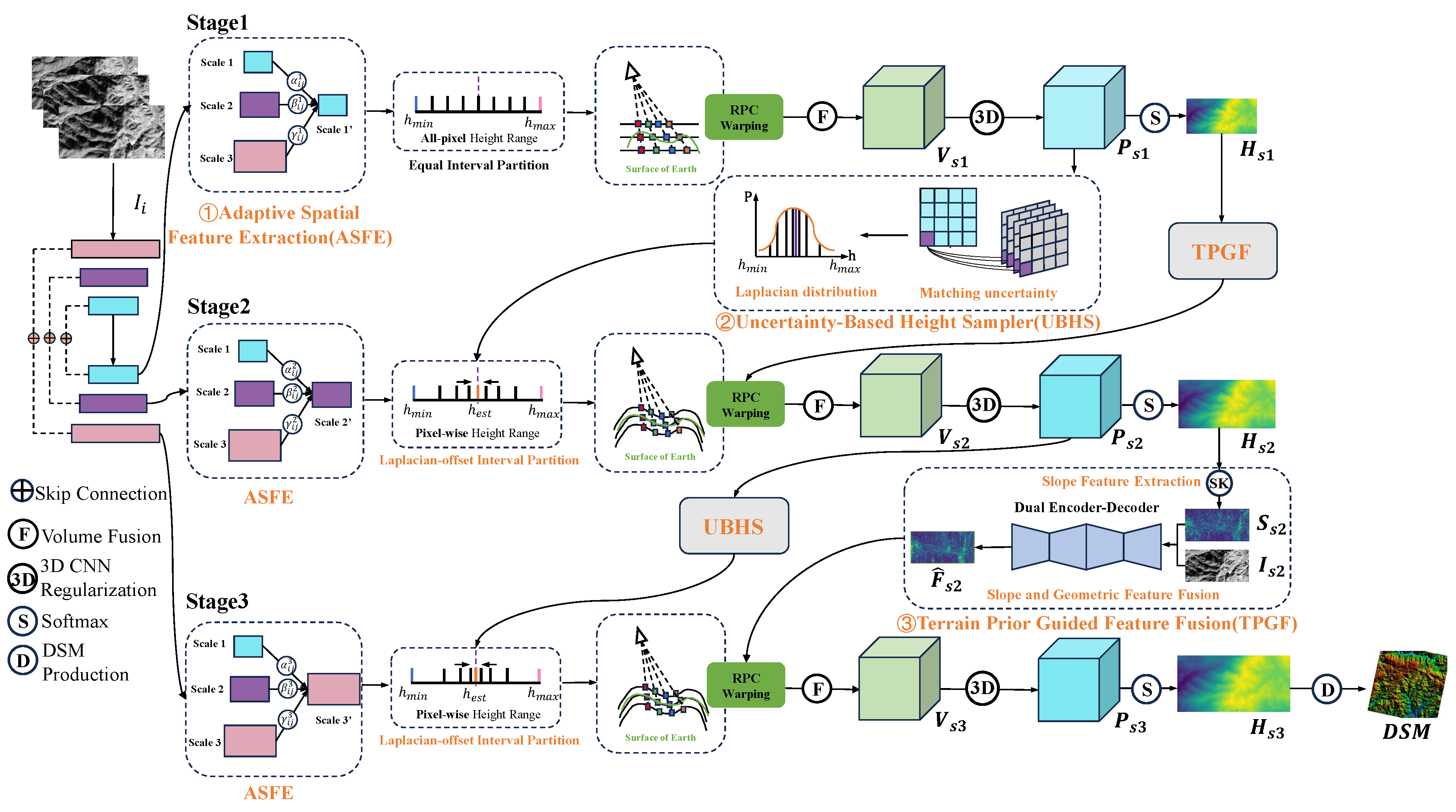
Figure 1. Illustration of the overall SA-SatMVS. Our network consists of feature extraction, cost volume construction, cost volume regularization, height map regression, and DSM production. This is a typical multi-stage coarse-to-fine framework. ASFE, UBHS, and TPGF are our novel modules. The baseline architecture is derived from the SatMVS(CasMVSNet) [5].
Remotesensing 16 03474 g001
Figure 2. Illustration of the adaptive spatial feature extraction network. The left, middle, and right parts represent the optimal integration of the three stages.
Remotesensing 16 03474 g002
Figure 3. Illustration of Slope−Net. The middle part is the SK Conv Layer. It contains two directional Sobel kernels.
Remotesensing 16 03474 g003
Figure 4. Comparison of the convolutional layers and geometric convolutional layers. A geometric convolutional layer augments a convolutional layer by concatenating three extra channels (X, Y, and Z) to the input.
Remotesensing 16 03474 g004
Figure 5. Illustration of the terrain-prior-guided feature fusion network. The middle part consists of dual encoder–decoder architecture. The right part contains the basic FPN network.
Remotesensing 16 03474 g005
Figure 6. The height map results of SatMVS (CasMVSNet), SatMVS (UCS-Net), SatMVS (RED-Net), and SA-SatMVS.
Remotesensing 16 03474 g006
Figure 7. The DSM results of SatMVS(CasMVSNet), SatMVS(UCS-Net), SatMVS(RED-Net), and SA-SatMVS.
Remotesensing 16 03474 g007
Table 1. Quantitative results on the height maps of the WHU-TLC-v2 dataset with different MVS methods which have employed the RPC warping.
MethodsMAE (m)<2.5 m (%)<7.5 m (%)
SatMVS (RED-Net)1.83682.0696.63
SatMVS (CasMVSNet)1.97981.8996.54
SatMVS (UCS-Net)1.87581.9696.59
SA-SatMVS1.70484.0296.77
Table 2. Quantitative results on the DSMs of the different MVS methods on the WHU-TLC dataset.
MethodsMAE (m)↓RMSE (m)↓<2.5 m (%)↑<7.5 m (%)↑Comp. (%)↑
Adapted COLMAP2.2275.29173.3596.0079.10
RED-Net2.1714.51474.1395.9181.82
CasMVSNet2.0314.35177.3996.5382.33
UCS-Net2.0394.08476.4096.6682.08
SatMVS (RED-Net)1.9454.07077.9396.5982.29
SatMVS (CasMVSNet)2.0203.84176.7996.7381.54
SatMVS (UCS-Net)2.0263.92177.0196.5482.21
SA-SatMVS1.8793.78579.0296.6282.37
Table 3. Ablation study on the WHU-TLC dataset (✓ represents that we use the corresponding novel module).
Modules
MethodASFEUBHSTPGFMAE (m)↓RMSE (m)↓<2.5 m (%)↑<7.5 m (%)↑Comp. (%)↑
-ASFE 1.9453.83378.7196.3182.31
-UBHS 1.9683.84178.4796.4582.29
-TPGF 1.9733.86378.3496.3782.21
SA-SatMVS1.8793.78579.0296.6282.37
Table 4. Quantitative results on the height maps of the WHU-TLC-v2 dataset with different kinds of functions which have employed RPC warping.
MethodsMAE (m)<2.5 m (%)<7.5 m (%)
SA-SatMVS (linear)1.78683.5996.61
SA-SatMVS (softmax)1.70484.0296.77
Table 5. Quantitative results on the DSMs of the different kinds of functions on the WHU-TLC dataset.
MethodsMAE (m)↓RMSE (m)↓<2.5 m (%)↑<7.5 m (%)↑Comp. (%)↑
SA-SatMVS (linear)1.9333.89478.5296.4782.16
SA-SatMVS (softmax)1.8793.78579.0296.6282.37
Disclaimer/Publisher’s Note: The statements, opinions and data contained in all publications are solely those of the individual author(s) and contributor(s) and not of MDPI and/or the editor(s). MDPI and/or the editor(s) disclaim responsibility for any injury to people or property resulting from any ideas, methods, instructions or products referred to in the content.