A New Framework for Generating Indoor 3D Digital Models from Point Clouds

Abstract

Three-dimensional indoor models have wide applications in fields such as indoor navigation, civil engineering, virtual reality, and so on. With the development of LiDAR technology, automatic reconstruction of indoor models from point clouds has gained significant attention. We propose a new framework for generating indoor 3D digital models from point clouds. The proposed method first generates a room instance map of an indoor scene. Walls are detected and projected onto a horizontal plane to form line segments. These segments are extended, intersected, and, by solving an integer programming problem, line segments are selected to create room polygons. The polygons are converted into a raster image, and image connectivity detection is used to generate a room instance map. Then the roofs of the point cloud are extracted and used to perform an overlap analysis with the generated room instance map to segment the entire roof point cloud, obtaining the roof for each room. Room boundaries are defined by extracting and regularizing the roof point cloud boundaries. Finally, by detecting doors and windows in the scene in two steps, we generate the floor plans and 3D models separately. Experiments with the Giblayout dataset show that our method is robust to clutter and furniture point clouds, achieving high-accuracy models that match real scenes. The mean precision and recall for the floorplans are both 0.93, and the Point–Surface Distance (PSD) and standard deviation of the PSD for the 3D models are 0.044 m and 0.066 m, respectively.

1. Introduction

The floor plans and 3D models of indoor scenes are widely used in fields such as indoor navigation, civil engineering, architectural design, and safety assessment [1,2,3]. The traditional method of obtaining floor plans and 3D models is mainly through manual measurement and the use of commercial software such as AutoCAD and Autodesk Revit for drawing. This is a time-consuming and labor-intensive task. With the development of LiDAR scanning technology [4,5], various types of laser scanning devices, such as consumer-grade RGBD (RGB and depth) sensors, lightweight terrestrial laser scanners (TLS), and hand-held laser scanning (HLS) or backpack laser scanning (BLS) devices, have been used for data acquisition of indoor scenes. RGBD images (e.g., Microsoft Kinect) acquired by a camera and a depth sensor are widely used in 3D visual applications. However, RGBD sensors are limited by their small scanning range and high level of noise. TLS scanners can obtain high-quality data but suffer from low mapping efficiency because of their laborious scan station resetting and registration procedures. By combining an inertial measurement unit (IMU) and simultaneous localization and mapping (SLAM) technologies, Mobile Laser Scanning (MLS) can continuously obtain high-precision and high-density point clouds while moving around. They can be applied to indoor scenes that have complex layouts and can minimize the effects of occlusions. Therefore, in recent years, there has been an increasing amount of research on the automated reconstruction of floor plans and 3D digital models from indoor point clouds. However, due to the complexity of indoor scenes and the disorderliness and noise of point clouds, achieving complete automation in reconstructing high-precision floor plans and 3D models from point clouds is a challenging task.

There are many methods [6,7,8] that firstly detect geometric primitives, vertices, lines, and planes, and then classify them to obtain permanent structures that make up the scene, such as walls, ceilings, doors, and windows. By assembling these structures, indoor scene models are generated. For example, Han et al. [7] extracted vertical and horizontal planes from point clouds by analyzing normal vectors, using vertical planes as walls, and distinguishing floors and ceilings by calculating the average height of horizontal planes. Walls are then used to generate floor plans. The building model is generated by stretching the floor plan and combining it with ceilings and floors. Sanchez et al. [8] used principal component analysis to divide the point cloud into five categories: ceiling point, floor point, wall X point, wall Y point, and remaining points. Plane fitting is performed for each category, and detection and modeling of stairs are performed on the remaining points. This type of method is bottom-up. It has poor robustness, and incomplete point clouds can lead to the loss of some structures, especially walls, resulting in reduced accuracy and incompleteness of the final generated model.

Some methods [6,9,10,11,12] improve robustness by dividing the space and reconstructing different rooms separately. For example, Tang et al. [11] projected point clouds onto the horizontal plane to create binary images, using morphological operations to divide space, and extracted boundaries from segmented spaces to generate floor plans, which were then used to create BIM. Cui, Y., et al. [6] analyzed the visibility of trajectory points to segment the space, constructing a vectorized model using multi-label graph cuts after segmentation. There are also methods [13,14,15] that use a slicing-based approach to detect planes in the scene and then transform the reconstruction task into a cell or plane selection problem by extending the supporting planes of each primary and partition 3D space into a set of polymeric cells or polymeric faces. Polyfit [14] used region-growing or RANSAC algorithms to detect planes in the point cloud, and then obtained a set of intersecting planes by extending the planes to the boundary of the point cloud. The user selects the plane by minimizing the energy function, which includes three terms: data fitting, model complexity, and point coverage. The final model is composed of the selected planes. KSR [13] utilizes a dynamic data structure to reduce reconstruction time by partitioning space into a convex polyhedral and extracting a seamless polymer mesh from the partitions using a minimum cut formula. These methods have strong robustness to indoor noise and can also reconstruct point clouds that are missing due to occlusion. However, this type of method reconstructs the entire scene as input, and the reconstructed model lacks semantic information and the topological relationship between rooms, which limits the application scope of the model.

Our method belongs to the category of spatial segmentation methods. We propose a new method for space partitioning. Firstly, we detect walls in the scene and project them onto the ground to generate line segments. Then, the line segments are extended to intersect and generate a set of candidate line segments. We select line segments to obtain initial spatial partitioning by minimizing a constraint-based energy function. After that, the selected line segments are converted into an image, and by using the image connectivity detection we obtain the room instance map. Our method is based on roof point clouds, as in indoor scenes, roof point clouds are often not obstructed by indoor debris and are saved relatively intact. We use the RandLA-Net [16] semantic segmentation network to extract the roof. We innovatively perform overlap analysis between the roof and room instance map to segment the roof point cloud for more accurate spatial partitioning. Through this, the entire roof is segmented into several different room’s roofs. We then extract and regularize their boundary points to obtain the polygonal boundaries of each room. Afterwards, we detect the doors and windows in the scene, a process which is divided into two parts. Firstly, we detect doors and windows at the boundary where the rooms are adjacent, reconstructing the topological relationships between the rooms, and generate a floor plan. Afterwards, we detect the doors and windows in other parts of the room, and finally generate a 3D digital model by stretching the floor plan and combining it with the detected doors and windows. Our main contributions include the following points:

(1)

A new method for spatial segmentation is proposed. This method firstly selects the walls of rooms by minimizing an energy function to generate the room instance map for initial spatial segmentation. Then, by innovatively performing an overlap analysis between the roof and room instance map, more accurate spatial segmentation can be obtained.

(2)

A new method for reconstructing the topological relationships between rooms is proposed. It firstly extracts potential areas that may exist as openings, which narrows down the detection range. Then, by performing density filtering, the precise position of the opening is detected. It then combines the opening with the boundary of the rooms to reconstruct the topological relationship between the rooms.

(3)

A method for detecting doors and windows in indoor scenes is proposed. It first detects openings on the boundaries of rooms, then classifies them as windows or doors by analyzing their length and height, and finally parameterizes them.

2. Related Works

In this section, we will summarize the relevant research on indoor reconstruction from point clouds. We will analyze several key technologies in the reconstruction process, including floor plan generation, spatial partitioning, and door and window detection.

2.1. Floor Plan Generation

Many methods [11,17,18] generate floor plans by extracting walls and projecting them onto the horizontal plane. Wang [19] used the RANSAC algorithm to detect wall planes and project them onto a plan to generate line segments and extended these line segments to obtain intersecting sets. Finally, they selected segments to generate floor plans. Okorn et al. [20] used the Hough transform to detect line segments from the projected wall point clouds. Tang [11] used a point cloud semantic segmentation network to extract walls in the scene, then projected them onto the ground to generate binary images, and by operating on these images, they generated floor plans. Kong [21] gridized the point cloud on the ground, and then detected the corner points by using a sliding window, and generated a floor plan by connecting the corner points. However, this method cannot extract the internal boundaries of buildings. Han [22] projected the wall point cloud onto the ground and divided the 2D space into vertices, edges, and faces using the KIPPI algorithm; they then used integer programming to extract the outer boundary of the building. By solving the Markov random field problem, they obtained the internal layout of the building. With the development of deep learning, many studies use neural networks to help generate the floor plan. Chen [23] inputted the density image of the point cloud to Mask-RCNN [24] to segment the rooms in the scene, thereby obtained room instance images, and then reconstructed the floor plan as multiple polygons using a room coordinate density algorithm. Wang [18] used CGAN [25] to optimize wall segments projected onto the ground to obtain regularized line segments, and finally generated a floor plan by assembling these line segments. Chen Liu [26] inputted 3D point cloud along with 2D point cloud density map and RGB image to an end-to-end network. They used three DNN branches to extract features, and employed the integer programming to recover the vectorized floor plan. Shang et al., predicted the 3D room layout of the Manhattan world from a single RGB panorama, using two projections of the panorama: an equal-area panorama view and a perspective ceiling view, used two network branches to analyze these projections, and then a novel feature fusion structure was proposed to connect these branches.

2.2. Space Partition

There are many methods for spatial partitioning, such as using ray casting to obtain free space evidence or morphological operations. Yang et al. [12] projected walls onto the horizontal plane to generate line segments, extended the line segments to obtain a cell complex, and performed overlap analysis between the cell complex and free space evidence to partition the indoor space. Similarly, Chen et al. [9] performed a subtraction operation on the semantic maps of the floor and walls to obtain the difference semantic map. Then, they apply mathematical morphology to obtain the room semantic map. By overlaying the room semantic map with the cell complex, they partition the space. Tang [11] projected the point cloud onto a 2D plane to generate a binary image, and then used morphological operations of the image to segment the space. There are also some methods that use the visibility of points to segment indoor spaces. Cui et al. [6] proposed a method based on analyzing the visibility of simulated trajectory points in the line of sight. They used detected door positions to limit the visible range of the point cloud, and then visibility clustering was performed on points with similar scanning trajectories to segment rooms in indoor scenes. Becker and Brunskill [27,28] firstly partitioned the space into a cell decomposition via extracted wall lines, and then they labeled each cell via an energy minimization approach. Chen [23] projected the point cloud onto the ground and generated a density image of the point cloud, and then inputted it into Mask-RCNN to obtain a segmented image of the room to partition the space.

2.3. Door and Window Detection

Due to the complexity of indoor environments and the presence of noise, door and window detection is a challenging task. Zhao, J et al. [29] sliced point clouds of different heights in the scene, projecting point clouds of the same slice onto the same plane, and performed overlap analysis on different slices to extract the position of the door. Liu et al. [30] projected the point cloud of the wall onto a plane which parallel to the wall and perpendicular to the XOY plane. By counting the number of pixels in each column, missing walls were filled in, and openings in the image were detected. Openings that met the length and width thresholds were selected as doors. Yang et al. [12] voxelized the point cloud and used ray-tracing to classify the voxels as occupied or empty. Openings were detected through the labeled voxels, and different viewpoints were selected to identify gaps for detecting doors and windows. Zuo et al. [31] used a point cloud semantic segmentation network to detect doors and windows in the scene, and added them to the generated BIM model by regularizing and parameterizing the doors and windows. Neural network-based methods require a large number of datasets and, due to the complexity and diversity of indoor scenes, predicting accurate point clouds for doors and windows in different styles of test data is a difficult task. Cheng et al. [32] projected the point cloud to horizontal planes to generate 2D point cloud data. The 2D point cloud data were then transformed to images representing the indoor area for feature extraction. On the 2D images, the 2D boundary of each potential opening was extracted using an improved Bounding Box algorithm, and the extraction result was transformed back to 3D data. Based on the 3D data, the reflectivity of the building materials was applied to differentiate windows and doors from potential openings, and the number of data points was used to check the opening condition of windows and doors. Díaz-Vilariño et al. [33] created a vertical point cloud profile through trajectories, and then detected the local minimum value of vertical distance to detect doors. Due to the timestamp association between point clouds and trajectories, this feature was used to segment point clouds into subspaces based on the position of doors.

3. Methodology

As shown in Figure 1, our method’s overall workflow begins with the input of voxel sampled point clouds. We firstly use RandLA-Net to extract the wall and roof point clouds and filter out wrong points by analyzing the normal vector of extracted points. Then, we detect planes in the wall point clouds and project them onto a horizontal plane to generate 2D line segments. By extending these line segments, we obtain a set of intersecting line segments. We need to select the line segments that form the rough boundary of the rooms from these segments. We transform the problem of selecting line segments into an energy minimization problem. As shown in Figure 1e, by minimizing the energy function E, we obtained the approximate layout of the rooms. We convert these lines into a raster image and use image connectivity detection to segment the regions, generating room instance maps. As shown in Figure 1f, different colors in the room instance map represents different room areas in the indoor scene. Next, we segment the planes in the extracted roof point clouds. We sequentially use RANSAC [34], Euclidean clustering, and region-growing [35] algorithms to segment the roof point clouds into small patches. By performing an overlap analysis between these patches and the room instance map, we obtain the roof point cloud for each room. Then, the Alphashape [36] algorithm is used to extract the boundaries of the roof point clouds for each room. After that, we simplify and regularize the ordered boundary points to generate boundary polygons for each room. The generated polygons are independent and do not have topological relationships between the rooms. We propose a method to detect openings that connect different rooms, reconstructs the topological relationships between rooms, and generates the floor plan of the scene. Finally, we detect the doors and windows in the scene and the heights of the walls. By combining the walls, doors, and windows, we generate the final 3D digital model.

3.1. Room Instance Map Generation

First, we compute the normal vectors of the input point cloud. We extract the points with normal vectors forming an angle close to 90° with the vertical direction (0, 0, 1) as the initial vertical point cloud. Then, we use the RANSAC algorithm to detect planes in the vertical point cloud. For each plane, we calculate its intersection line with the ground and project the points on the plane onto this intersection line, taking the two furthest points on the line as the endpoints of the segment. We obtain segments projected onto the ground for each plane.

These segments are discrete, so we extend them to intersect, forming a segment set S and the vertices of all segments V, where each vertex is shared by two or more segments. The connection matrix between vertices and segments is M. We select segments by minimizing a constraint-based energy function E, as shown in Equation (1),

$$E=1-{\displaystyle \frac{1}{N}}\cdot {\displaystyle \sum _{i=1}^N\left(\max \left\{1,\frac{N_{Si}}{\delta \cdot L_i}\right\}\cdot s_i\right)}$$

(1)

where s_i represents each segment and takes a value of 0 or 1, for which s_i = 0 means the segment is discarded and s_i = 1 means the segment is retained. L_i is the length of segment s_i, and δ is a fixed density value defined per unit length to have δ points. N_Si is the number of support points for the segment. Our method is inspired by Wang’s work [19], but we only use the confidence term as the energy component since we do not need a strictly regular floor plan. The confidence term filters out segments with insufficient support points. Additionally, we add constraints on the vertices to ensure a closed floor plan, as shown in Equation (2),

$${\displaystyle \sum _{s_i\in S_{v_j}}{s}_i=0or2or3or4},\forall v_j\in V$$

(2)

to obtain a closed space partition map, where V represents the intersection points of all segments. S_vj is the set of segments connected to intersection point $v_j$. We minimize Equation (1) with Equation (2) as a constraint using the SCIP solver. Then, the floor plan is obtained by selecting wall candidate segments with s_i = 1.

After obtaining the space partition map, we convert it into a raster image and use connectivity segmentation to segment the regions. As shown in Figure 2e, we use different colors to represent different rooms in the scene. We do not need strictly accurate room boundaries, just a rough partition of the indoor space. The precise reconstruction of room boundaries will be carried out later.

3.2. Roof Point Cloud Segmentation

We firstly use the RandLA-Net point cloud semantic segmentation network to extract the roof of the input point cloud. Due to the lack of color information in the input point cloud, the output of the network includes some furniture and ground points in addition to the roof. Therefore, we calculate the roof height of the scene and filter out points below 2/3 of the roof height. We first use the RANSAC algorithm to perform plane detection on the roof point cloud. However, since the RANSAC algorithm may merge discontinuous but coplanar planes into the same class, this can lead to incorrect roof segmentation. Therefore, after RANSAC segmentation, we use Euclidean clustering to separate the non-contiguous planes detected by RANSAC. Finally, we use region-growing segmentation on each category obtained from the previous steps to segment more patches, as we will later merge patches belonging to the same room. As shown in Figure 3a, the roof point cloud is segmented by three methods. We perform an overlay analysis with the previously obtained room instance map to merge the roof point clouds belonging to the same room. We project the point cloud onto the room instance map. For each plane, we calculate the pixel proportion it occupies in different rooms of the room instance map and record the room with the highest proportion as the room to which the plane belongs, as shown in Formulas (3) and (4):

$$C_i=clas{s}_{id}$$

(3)

$$id=t,if({n_s}^t)=\max \left\{{\displaystyle \frac{n_s^{id}}{h}}\right\},id\in L,L=\{1,2,3\dots m\}$$

(4)

where C_i represents the label of the room each plane belongs to, class_id represents different types of room pixels, h is the total number of pixels the plane projects onto the room instance map, and m is the number of different types of pixels. Once the planes are labeled, we merge planes belonging to the same room into one category. As shown in Figure 3c, we use different colors to represent the point clouds of different rooms after the overlay analysis.

3.3. Room Boundary Extraction

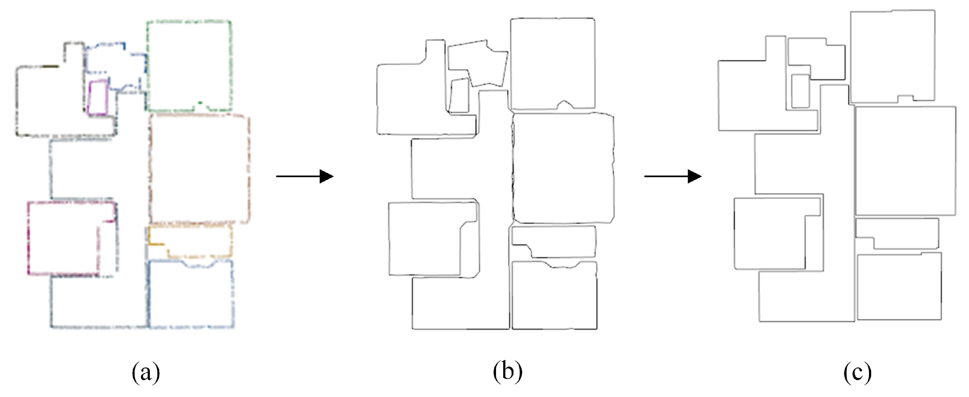
After obtaining the roof point cloud for each room, we use the Alphashape algorithm to extract the ordered boundary points of each room’s roof. Shown in Figure 4a are the boundary points we extracted. By sequentially connecting the ordered boundary points, we obtain closed polygons representing the room boundaries. However, the boundary points extracted by the Alphashape algorithm contain many redundant points and are not regularized. Therefore, we simplify the boundary points using the polygon simplification algorithm proposed by Dyken [37]. This method simplifies the polygon by gradually replacing the edge (p, q) and edge (q, r) with edge (p, r) and removing vertex q from the polyline. During the simplification process, the topological structure of the line set is maintained. After obtaining the simplified boundary points, we sequentially connect them to form closed polygons. We then regularize these boundary polygons. We take the direction of the longest wall segment from the previously projected wall segments as the primary direction of the building, and the two directions at 45° to it as the other two primary directions. We use these three primary directions as inputs to the polygon regularization algorithm in CGAL to regularize the boundary polygons of each room. This algorithm iterates through each edge, adjusting its direction to the nearest primary direction and removing redundant points. As shown in Figure 4c, the polygons are the room boundaries after regularization.

3.4. Door and Window Detection

3.4.1. Adjacent Boundaries Extraction

We have obtained the boundary polygons for each room, but these polygons are independent and lack the topological relationships between rooms. In this section, we reconstruct the topological relationships by detecting doors and windows in the scene, extracting more semantic information. Our detection process is divided into two parts. The first part is to detect the doors and windows at the boundary where the rooms are adjacent. The doors and windows at the adjacent boundary play a role in connecting the two rooms. The second part is to detect doors and windows at other boundaries. We may have different treatments for the doors and windows detected in the two parts when rebuilding the 3D model.

First, we detect the doors and windows that connect rooms. We find that these doors and windows are located at the boundaries between adjacent rooms. Therefore, we first detect the positions of the adjacent boundaries between the rooms. For each edge of the room boundary, we traverse other boundary segments that do not belong to the same room. If these two segments are parallel and the distance is less than a certain threshold, we project the endpoints of these two segments onto the line located in their middle position. If these two segments overlap, we further extract the overlapping parts and call them adjacent boundaries. We mark these two segments as processed. As shown in Figure 5, the red line segments shown in the figure represent the adjacent boundaries we have extracted.

3.4.2. Opening Detection

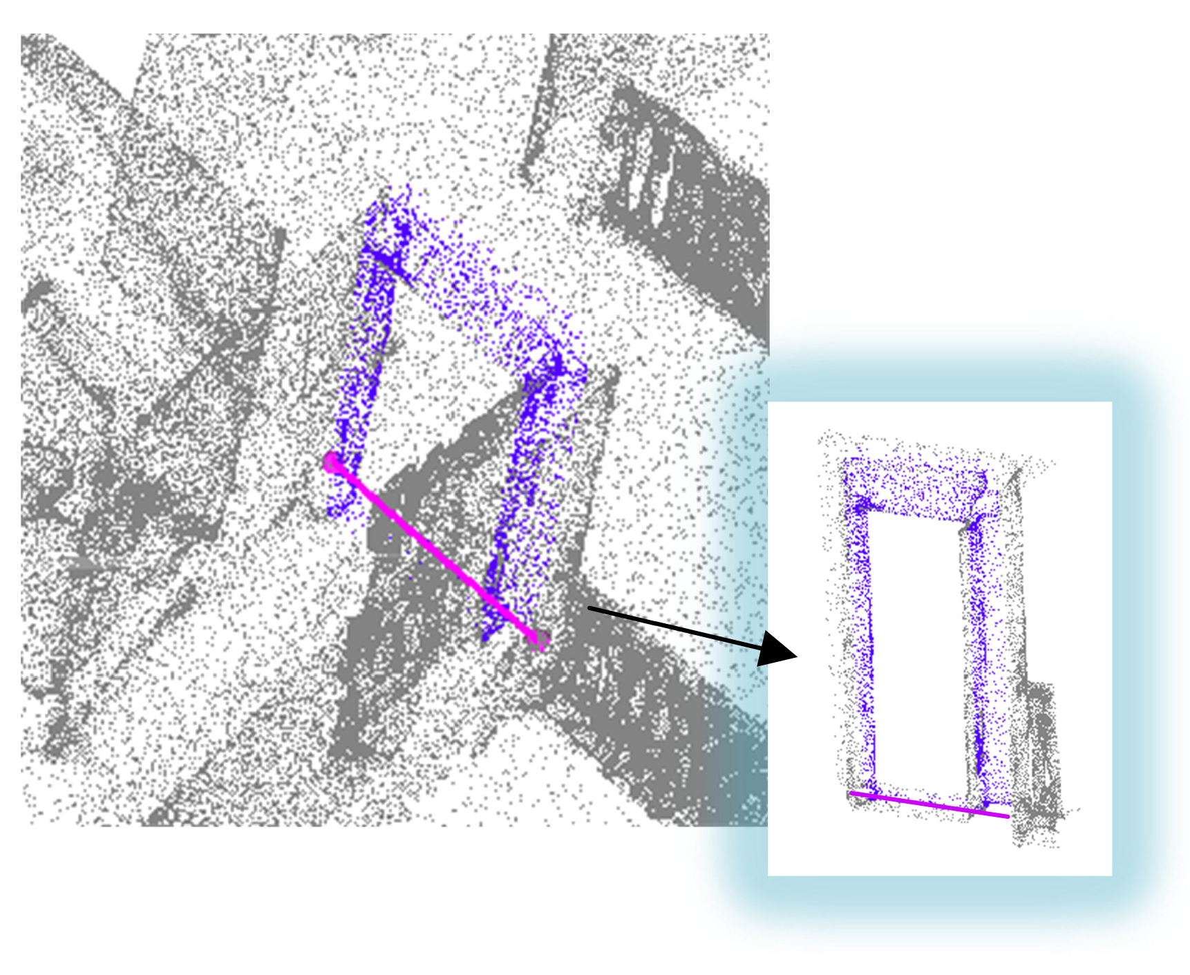
After extracting the adjacent boundaries, we detect the doors and windows at the adjacent boundaries. As shown in Figure 6, we project the points in the original point cloud with x and y coordinates close to the adjacent boundary and located between the two endpoints of the boundary onto the boundary. The purple line segments represent the adjacent boundaries, and the blue points represent the points to be projected onto the adjacent boundaries. After projection, we divide the segment into multiple small intervals, setting the number of intervals to 100. We perform density filtering for each interval: if the number of points in an interval is less than a set threshold, we filter out all points in that interval. Due to the presence of voids in the position of doors and windows, the number of points projected onto the line segment is significantly smaller than the surrounding area. Therefore, after density filtering, there will be a blank space in the position of doors and windows on the line segment. As shown in Figure 7, Figure 7a shows the points on the line segment before density filtering and Figure 7b shows the points on the line segment after density filtering. We will sort the filtered points according to the direction of the line segment, and then calculate the distance between adjacent points in sequence. If the distance between two points is greater than 0.5 m, we will mark these two points as the position of the opening, as shown in Figure 8. The distance between the two red points in the figure is greater than 0.5 m. We will save these two points as the two endpoints of the opening line segment, and the vertical coordinates of these two points are 0.

3.4.3. Classification of Doors and Windows

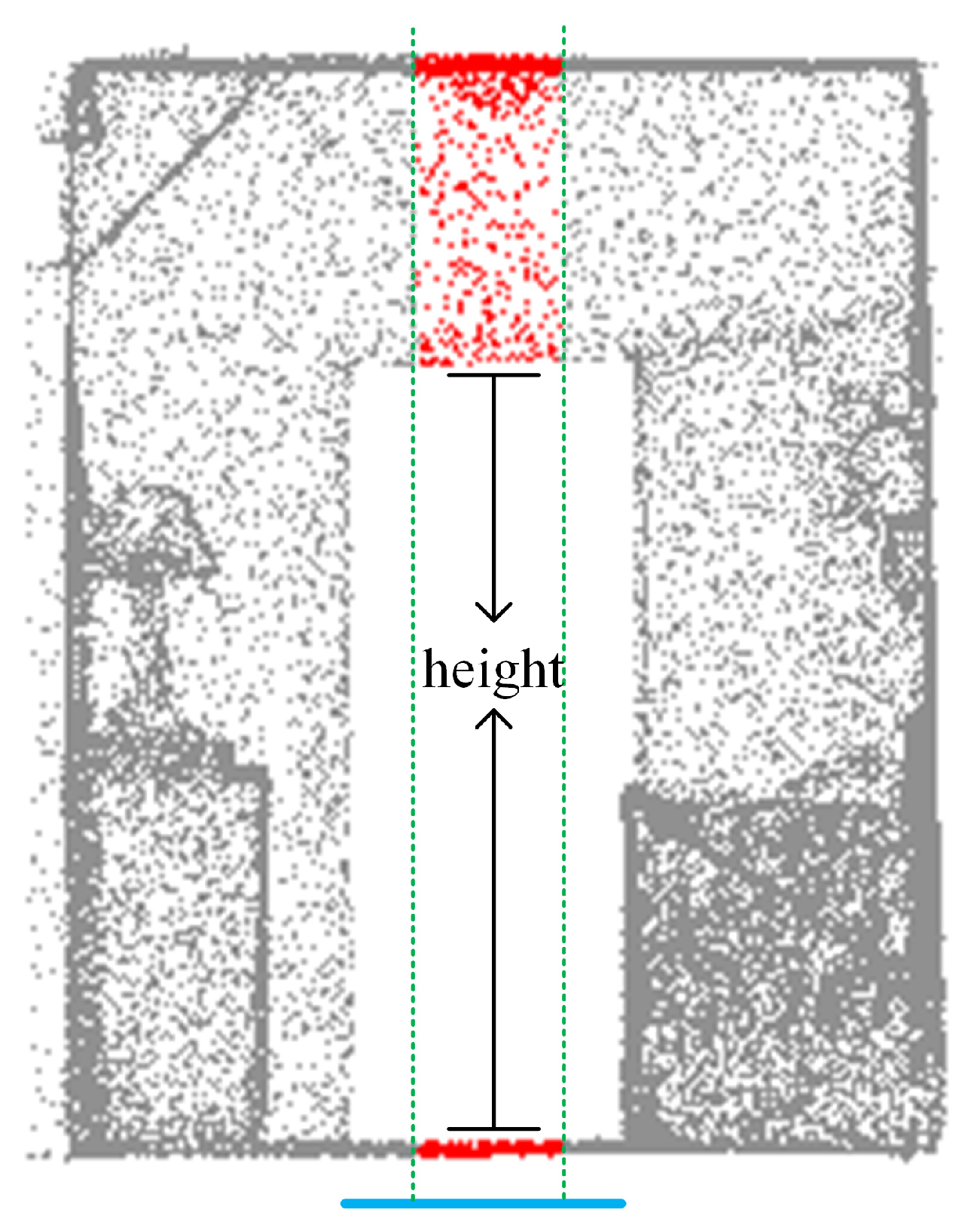
After all openings have been detected, we construct planes perpendicular to the ground using each opening segment. As shown in Figure 9, blue lines represent the openings. To avoid the influence of points on the edges of openings on height detection, as shown by the dashed lines in the diagram, we take a middle section of the opening segment to construct a plane perpendicular to the ground. Points near this plane from the original point cloud are projected onto the plane. Subsequently, we sort the vertical coordinates of the points on the plane. Similarly, we calculate the distance between adjacent points sequentially. When the distance exceeds a certain threshold, we record this distance as the height of the opening and mark these two points as p₃ and p₄, where the vertical coordinate of point p₃ is less than that of point p₄. We use the height to determine whether the opening is a door or window. If the lowest point between the two points is close to the ground and the distance between them exceeds 1.5 m, we classify this opening as a door. If the lowest point is not close to the ground, we classify it as a window.

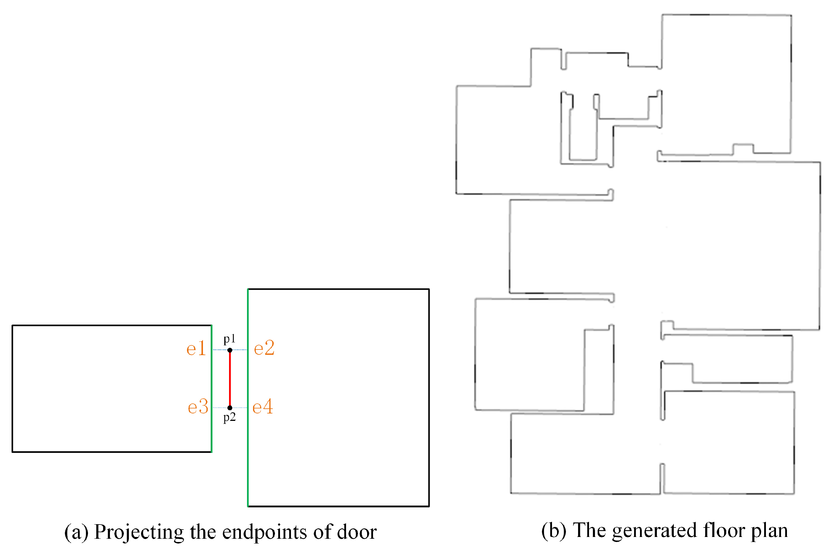
After obtaining the position of the door at the adjacent boundary, as shown in Figure 10a, we project the two endpoints p₁ and p₂ of the door onto the two closest room boundaries l₁ and l₂ respectively to obtain four endpoints e₁, e₂, e₃, and e₄. The red line segment in the figure is the door, and the green line segments are the two nearest boundaries to the door. We connect e₁, e₂, and e₃, e₄ respectively to connect the two adjacent rooms, and remove the line segments (e₁, e₃) and (e₂, e₄), so that the door will appear as an opening in the floor plan. The floor plan we generated is shown in Figure 10b.

Previously, we marked the room boundaries located at adjacent areas and detected the doors and windows. Next, we detect the doors and windows at other locations. The reason for separating the two is that we process them differently in the subsequent generation of 3D model. The method of detecting doors and windows is the same as before, but we do not detect them through adjacent boundaries. Instead, we detect the doors and windows through the room boundaries marked as unprocessed.

3.5. 3D Digital Model Generation

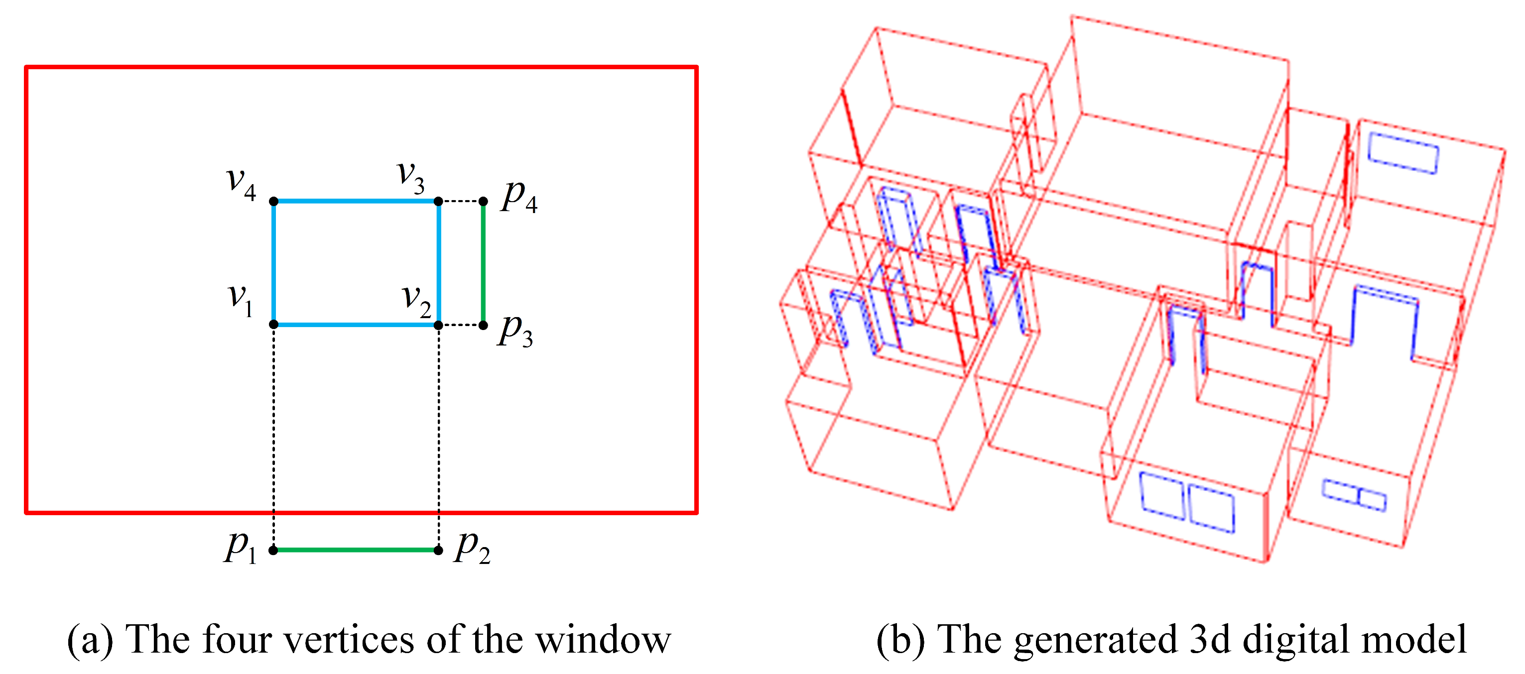
After obtaining the floor plan and door and window information of the building, we generate a 3D model by extruding the floor plan to a specified height and incorporating the detected doors and windows to create the final model. We first detect the height of the room boundaries by calculating the average height of the roof point cloud for each house boundary. We stretch the house boundaries in the floor plan to the corresponding height to generate the 3D model. Afterwards, we added the door to the model. As we had previously recorded the height and position of the door, we stretched it to the saved height. It is worth noting that the door at the adjacent boundary is composed of two-line segments while the door at other boundaries of the house only has one line segment. We stretch the two-line segments to the same height and connect the corresponding vertices to reconstruct the door into a box. For reconstructing windows, we previously recorded the positions of the windows on both the horizontal and vertical planes. On the horizontal plane, the window’s position is represented as (p₁, p₂), and on the vertical plane, the window’s position is represented as (p₃, p₄), as shown in Figure 11a. We represent the window as a rectangle (v₁, v₂, v₃, v₄), where the length of the rectangle corresponds to the length of segment (p₃, p₄) and the width corresponds to the length of segment (p₁, p₂). We construct the four vertices of the rectangle with coordinates v₁(x₁, y₁, z₃), v₂(x₂, y₂, z₃), v₃(x₂, y₂, z₄), and v₄(x₁, y₁, z₄), where (x_i, y_i, z_i) represents the x, y, and z coordinates of the point p_i (i = 1, 2, 3, 4). We then connect the four vertices v₁, v₂, v₃, and v₄ sequentially to form the polygon representing the window. As shown in Figure 11b, the generated 3D digital model features blue polygons representing doors and windows, and red polygons representing walls.

4. Experiments

We tested our algorithm using five scenes from the Giblayout dataset provided by Wang [19], which are common indoor buildings, including non-Manhattan scenes. We presented the floor plan and 3D model generated by our method, evaluated the accuracy and recall of room boundaries in the floor plan, and compared the generated floor plan with two deep learning-based methods. All of our algorithms were implemented in the C++ language and used the PCL v1.12.1 (point cloud library) and CGAL Library v5.5.2. All experiments were run on a PC with a 4-core Intel Xeon CPU (3.7 GHz) and an NVIDIA GTX 3060 GPU.

4.1. Dataset

The Giblayout dataset comprises 80 house models, each containing 3 to 10 rooms, totaling more than 10,000 square meters. The point clouds of the house models in this dataset were extracted from the publicly available Gibson Dataset [5], collected by NavVis (For more details visit https://www.navvis.com/zh/vlx (accessed on 1 November 2021)). NavVis employs two multi-layer LiDAR sensors and industry-leading SLAM algorithm software to generate mapping-quality point clouds. We performed voxel sampling on the input point cloud to reduce the number of points and balance the density of points.

4.2. Experimental Result

In this section, we presented the experimental results of our method on test data, and for each scenario, we reconstructed its floor plan and 3D digital model. As shown in Figure 12, Figure 12a represents the input point cloud and Figure 12b,c represent the results of visualizing the 3D digital model from different perspectives. From the results, it can be seen that our reconstructed floor plan not only reconstructs the boundaries of the rooms, but also contains the topological relationships between the rooms. This enhances our perception of the scene. The reconstructed 3D digital model has a high degree of overlap with the original scene, and the height of the reconstructed walls is not assumed, but based on roof detection, which makes the model more realistic. The reconstructed doors and windows enrich the semantic information of the model, which enables the model to be applied in more fields.

4.3. Comparison

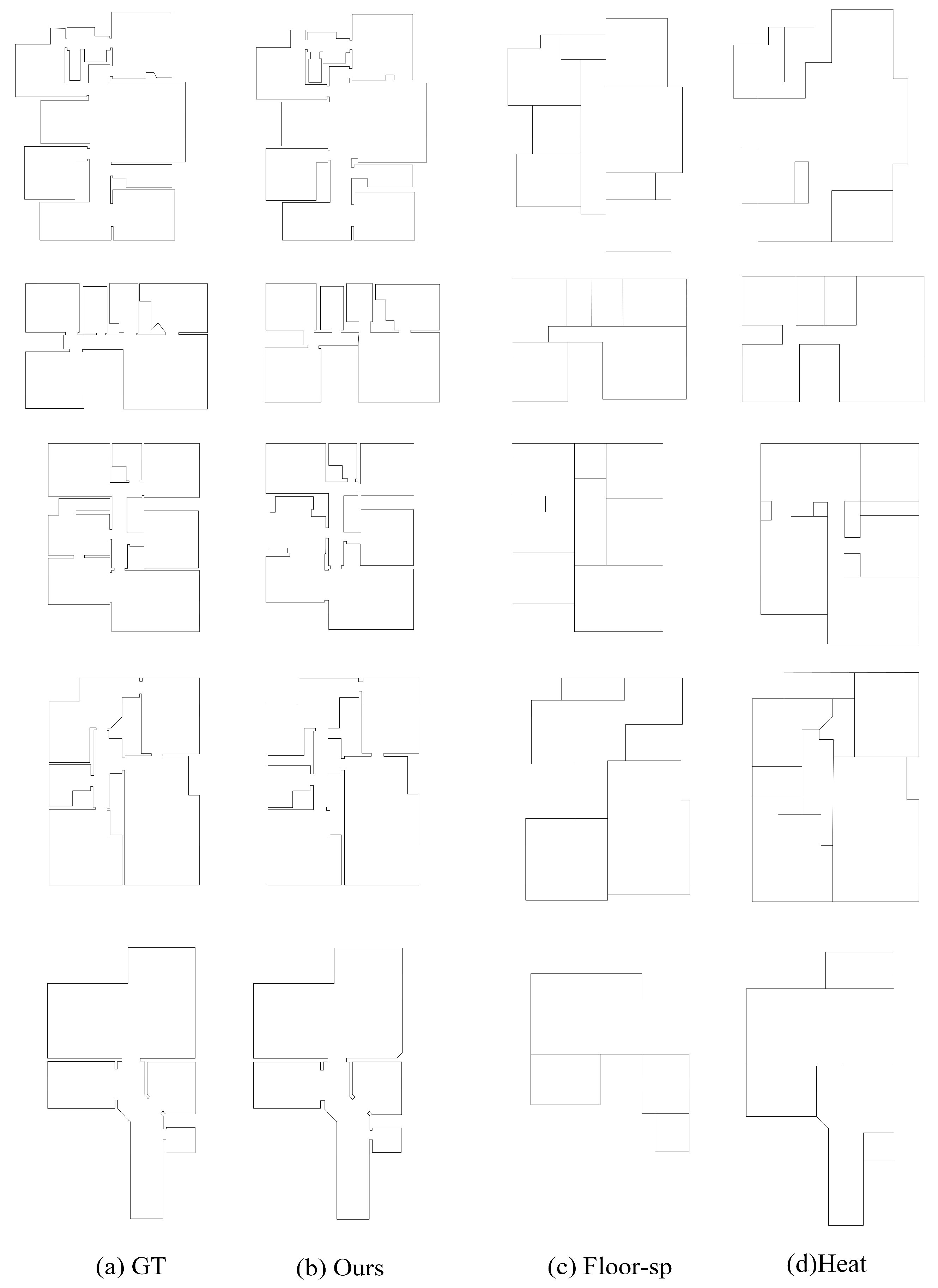
We compared our generated planar graph with two deep learning-based methods, namely Floor-sp and Heat. Floor-sp is a classic method of generating floor plans. It initially divides the building into multiple rooms, represents each room with a closed polygon, and then optimizes the room plan’s structure by solving the shortest path problem in descending order of room coordinates. Heat utilizes a novel neural network based on attention mechanisms for structural reconstruction. This method detects corner points in an end-to-end manner and classifies edge candidates between corner points. We will use the manually drawn floor plan as the Ground Truth (GT). As shown in Figure 13, from left to right are GT, the floor plan reconstructed by our method, the floor plan reconstructed by Floor-sp, and the floor plan reconstructed by Heat. From the results, it can be seen that our method reconstructs the floor plan with more complete walls, and we are able to display the openings in the scene, which allows us to obtain the topological relationships between the rooms. Floor-sp and Heat can obtain more accurate spatial divisions, but they cannot reconstruct accurate house boundaries, and it is difficult to reconstruct openings in their scenes, which cannot reflect the topological relationships between rooms, which reduces the perception ability of the scenes.

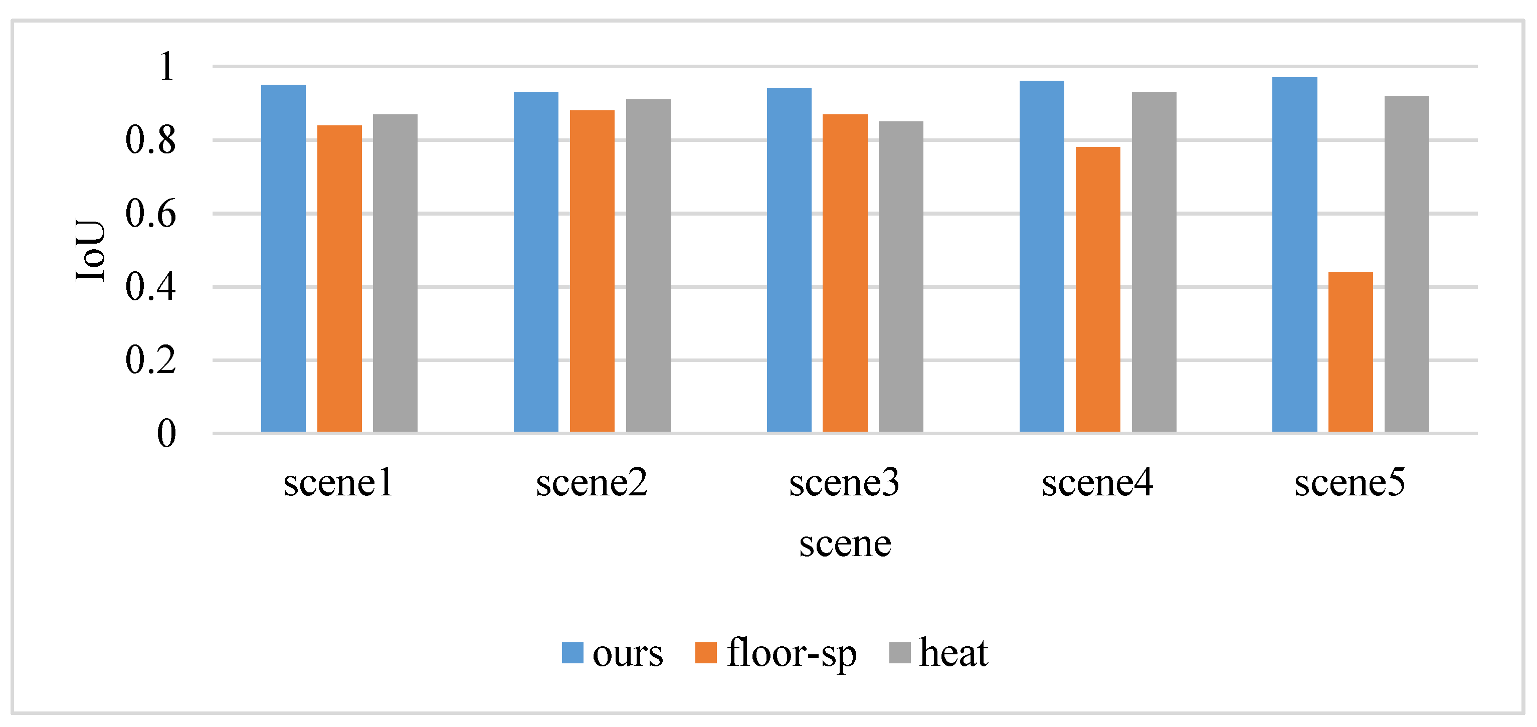
We also compared the IoU (Intersection over Union) metrics of the floor plans reconstructed by various methods with the GT, as shown in Figure 14. The IoU metrics we calculated indicate that our reconstructed floor plans have a higher IoU across all test data compared to the other two methods. This demonstrates that our method can reconstruct floor plans that have a high degree of overlap with the original scene.

4.4. Evaluation Metrics

The 3D digital model walls we generated were created by stretching the boundaries from the floor plan. The reconstruction effect of the boundaries in the floor plan can reflect the reconstruction effect of the walls in the 3D digital model. As shown in Formulas (5) and (6),

$$\mathrm{precision}={\displaystyle \frac{edg{e}_{correct}}{edg{e}_{res}}}$$

(5)

$$\mathrm{recall}={\displaystyle \frac{edg{e}_{correct}}{edg{e}_{gt}}}$$

(6)

We use two metrics, the precision and recall rate of the reconstructed room boundaries, to evaluate the floor plan. edge_res represents the total number of edges in our reconstructed floor plan, and edge_correct represents the number of correct boundaries in the reconstruction. We calculate the distance between the endpoints of the reconstructed boundaries and the endpoints in the GT. If the distance is less than 0.1 m, we consider the boundary as correctly reconstructed. edge_gt represents the total number of boundaries in the GT. As shown in

Table 1. The floor plans’ precision and recall rate of our method on the GibLayout dataset.

	Scene1	Scene2	Scene3	Scene4	Scene5	Mean
Precision	0.89	0.91	0.95	0.95	0.95	0.93
Recall	0.96	0.88	0.95	0.90	0.97	0.93

, we present the precision and recall rate of the reconstructed floor plans in five scenarios. From the table, it can be seen that we can reconstruct floor plans with a high degree of overlap with the original scenarios, with the average precision and recall on the test data both reaching 0.93. In scene1, the difference between precision and recall is 0.07. This is because in narrow areas, regularization of boundary points may generate redundant short edges, causing a decrease in accuracy.

We use the Point–Surface Distance (PSD) and standard deviation of the PSD (PSD_std) to evaluate the reconstruct 3D model. The PSD can reflect the shape similarity between the reconstructed model and point cloud. It calculates the average distance from the point cloud to the reconstructed model surface. The smaller the PSD, the closer the shape of the reconstructed model is to the point cloud. As shown in

Table 2. The PSD(m) and PSD_std(m) of reconstructed models.

	Scene1	Scene2	Scene3	Scene4	Scene5	Mean
PSD	0.028	0.037	0.055	0.049	0.053	0.044
PSDstd	0.031	0.047	0.103	0.058	0.090	0.066

, the mean PSD and standard deviation of the PSD of five reconstructed models were 0.044 and 0.066, respectively, which are both lower than 0.1. This indicates that the shape of the reconstructed model is very well restored and close to the shape of the point clouds.

We also evaluated the reconstruction of the doors in the scenes. We counted the number of reconstructed doors and the number of correctly reconstructed doors, as shown in

Table 3. The statistical results of reconstructed doors.

Scene	doorres	doorcorrect	doorgt
scene1	7	7	7
scene2	5	5	6
scene3	8	7	8
scene4	5	5	5
scene5	5	5	5

, where door_res represents the number of doors we reconstructed and door_correct represents the number of correctly reconstructed doors. When the length and width of the reconstructed doors and the distance between the plane of the door and the corresponding door in the GT are less than 0.1 m, we consider the door to be correctly reconstructed. door_gt represents the number of doors in the GT. It can be seen that our method can completely and accurately reconstruct the doors in the scenes.

Similarly, we also counted the reconstruction of windows, as shown in

Table 4. The statistical results of the number of reconstructed windows.

Scene	windowres	windowcorrect	windowgt
scene1	5	5	7
scene2	3	3	3
scene3	5	5	6
scene4	7	7	8
scene5	3	2	4

, where window_gt represents the number of windows in the GT, window_res represents the number of windows we reconstructed, and window_correct represents the number of correctly reconstructed windows. Our method may miss some windows that are closely attached to the walls during detection, and we will discuss this later.

5. Parameters Setting and Analysis

In this section, we analyze the key parameters in the reconstruction process. In fact, the parameters in our method are highly correlated with the density of the point cloud. Therefore, we use voxel sampling to preprocess the input point cloud. Voxel sampling can reduce the number of points and can adjust the point cloud density to our required range. In the experiment, we set the voxel size to 0.05 m. When minimizing the energy function to selected line segments, the number of support points per unit length affects the selection of line segments, which directly influences the subsequent generation of room instance maps. Since we performed voxel sampling on the point cloud, we can obtain an approximate range of 20 points per meter for unit length, so we set this parameter to 15–20. When extracting boundaries for the roof, we set the radius of the alpha shape algorithm to 0.15 m. Since we will later simplify and regularize the boundary points, the experimental results are not sensitive to this parameter. When performing density filtering on points on adjacent boundaries, the threshold for the number of points and the number of intervals which the line segment is divided will affect the detection of openings. In our experiments, we set the number of intervals to 100 and the threshold for the number of points to 15. The setting of the threshold for the number of points is related to the distance from the top of the opening to the roof. We can roughly calculate this distance and divide it by the size of the voxel to obtain a reference value. Then, we can set the threshold slightly larger than the reference value. When distinguishing doors and windows from openings, we set the criterion that if the height of the opening’s lowest endpoint from the ground is less than 0.2 m, we classify the opening as a door; otherwise, it is classified as a window. This is because windows are usually at a certain height from the ground, while doors are usually connected to the ground. Considering the existence possibility of a sill, we set this value to 0.2 m.

6. Discussion

Our method can reconstruct floor plans and 3D digital models with high overlap with real scenes, but there are still some areas that need improvement. Next, we will discuss several key issues encountered in the experimental process.

(1)

Roof Point Cloud Extraction: Since our method is based on the roof, we need to completely extract the roof point cloud. In this experiment, we used the RandLA-Net point cloud semantic segmentation network to extract the roofs in the scenes. We used the pretrained weights of this network on the S3DIS dataset to predict our data. However, due to the lack of color information in our point cloud, the extraction effect of roofs in some scenes was not satisfactory. We hope to use a dataset without color information for roof extraction training in the future, which would expand the applicability of our method.

(2)

Door Detection: Since our method reconstructs doors by detecting openings, we can only detect open doors. When doors are closed or obstructed by people, our method fails. We need to manually trim the point cloud at the door locations to correctly detect the doors. Traditional methods and emerging deep learning methods often lack robustness in door detection. The detection results are often unsatisfactory when facing different datasets, so door detection remains an issue for further research.

(3)

The reconstruction of curve structure: Our method can reconstruct common indoor scenes, including layouts such as rings, corridors, and non-Manhattan scenes, but it cannot reconstruct the curve structure in the scene. We plan to introduce curve and surface fitting algorithms to reconstruct more abundant structures.

(4)

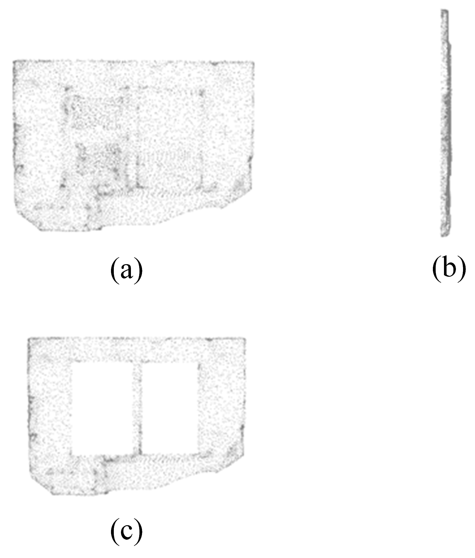
Window Detection: Similarly, for windows closely attached to walls, our method may fail. As shown in Figure 15, when the distance between the window and the wall is small, the point density on the projected line segment is very similar. This makes it difficult to filter out the points at the window location during density filtering, leading to undetected openings. Therefore, to fully detect window positions, it is necessary to trim such windows to create gaps, allowing our method to detect the openings.

7. Conclusions

We propose a method for reconstructing building floor plans and 3D digital models from indoor point clouds. First, we detect the wall point cloud and project it onto the ground to obtain a set of line segments. Then, we solve an integer optimization problem to select line segments and use connectivity segmentation to obtain room instance maps. Next, we use RandLA-Net to predict the roof point cloud, and perform an overlap analysis of the roof point cloud and the room instance maps to segment the roof point cloud. After that, we extract and regularize the boundaries of the roof point cloud to obtain room boundary polygons. By detecting doors and windows, we generate the floor plans and 3D digital models.

Different from other common methods, the proposed method is based on roofs, so it cannot be affected by indoor clutter and furniture points. We innovatively perform an overlap analysis between the roof and room instance map to segment the entire roof to get different rooms’ roofs. To reconstruct the topological relationships between the rooms, a new and robust method was proposed to detect the doors. It firstly extracts potential areas that may exist the door, which narrows down the detection range and reduces the interference of point clouds from other areas. In addition, we also reconstruct the windows in the scene, which enriches the semantic information of the model and expands its application scope.

References

1. Cerovsek, T. A review and outlook for a ‘Building Information Model’(BIM): A multi-standpoint framework for technological development. Adv. Eng. Inform. 2011, 25, 224–244. [Google Scholar] [CrossRef]
2. Hu, R.; Huang, Z.; Tang, Y.; Van Kaick, O.; Zhang, H.; Huang, H. Graph2plan: Learning floorplan generation from layout graphs. ACM Trans. Graph. 2020, 39, 118:1–118:14. [Google Scholar] [CrossRef]
3. Yang, J.; Kang, Z.; Zeng, L.; Akwensi, P.H.; Sester, M. Semantics-guided reconstruction of indoor navigation elements from 3D colorized points. ISPRS J. Photogramm. Remote Sens. 2021, 173, 238–261. [Google Scholar] [CrossRef]
4. Wen, C.; Qin, L.; Zhu, Q.; Wang, C.; Li, J. Three-dimensional indoor mobile mapping with fusion of two-dimensional laser scanner and RGB-D camera data. IEEE Geosci. Remote Sens. Lett. 2013, 11, 843–847. [Google Scholar]
5. Xia, F.; Zamir, A.R.; He, Z.; Sax, A.; Malik, J.; Savarese, S. Gibson env: Real-world perception for embodied agents. In Proceedings of the IEEE Conference on Computer Vision and Pattern Recognition, Salt Lake City, UT, USA, 18–22 June 2018; pp. 9068–9079. [Google Scholar]
6. Cui, Y.; Li, Q.; Yang, B.; Xiao, W.; Chen, C.; Dong, Z. Automatic 3-D reconstruction of indoor environment with mobile laser scanning point clouds. IEEE J. Sel. Top. Appl. Earth Obs. Remote Sens. 2019, 12, 3117–3130. [Google Scholar] [CrossRef]
7. Han, J.; Rong, M.; Jiang, H.; Liu, H.; Shen, S. Vectorized indoor surface reconstruction from 3D point cloud with multistep 2D optimization. ISPRS J. Photogramm. Remote Sens. 2021, 177, 57–74. [Google Scholar] [CrossRef]
8. Sanchez, V.; Zakhor, A. Planar 3D modeling of building interiors from point cloud data. In Proceedings of the 2012 19th IEEE International Conference on Image Processing, Orlando, FL, USA, 30 September–3 October 2012; IEEE: New York, NY, USA, 2012; pp. 1777–1780. [Google Scholar]
9. Chen, D.; Wan, L.; Hu, F.; Li, J.; Chen, Y.; Shen, Y.; Peethambaran, J. Semantic-aware room-level indoor modeling from point clouds. Int. J. Appl. Earth Obs. Geoinf. 2024, 127, 103685. [Google Scholar] [CrossRef]
10. Ikehata, S.; Yang, H.; Furukawa, Y. Structured indoor modeling. In Proceedings of the IEEE International Conference on Computer Vision, Santiago, Chile, 7–13 December 2015; pp. 1323–1331. [Google Scholar]
11. Tang, S.; Li, X.; Zheng, X.; Wu, B.; Wang, W.; Zhang, Y. BIM generation from 3D point clouds by combining 3D deep learning and improved morphological approach. Autom. Constr. 2022, 141, 104422. [Google Scholar] [CrossRef]
12. Yang, F.; Li, L.; Su, F.; Li, D.; Zhu, H.; Ying, S.; Zuo, X.; Tang, L. Semantic decomposition and recognition of indoor spaces with structural constraints for 3D indoor modelling. Autom. Constr. 2019, 106, 102913. [Google Scholar] [CrossRef]
13. Bauchet, J.-P.; Lafarge, F. Kinetic shape reconstruction. ACM Trans. Graph. 2020, 39, 1–14. [Google Scholar] [CrossRef]
14. Nan, L.; Wonka, P. Polyfit: Polygonal surface reconstruction from point clouds. In Proceedings of the IEEE International Conference on Computer Vision, Venice, Italy, 22–29 October 2017; pp. 2353–2361. [Google Scholar]
15. Oesau, S.; Lafarge, F.; Alliez, P. Indoor scene reconstruction using feature sensitive primitive extraction and graph-cut. ISPRS J. Photogramm. Remote Sens. 2014, 90, 68–82. [Google Scholar] [CrossRef]
16. Hu, Q.; Yang, B.; Xie, L.; Rosa, S.; Guo, Y.; Wang, Z.; Trigoni, N.; Markham, A. Randla-net: Efficient semantic segmentation of large-scale point clouds. In Proceedings of the IEEE/CVF Conference on Computer Vision and Pattern Recognition, Seattle, WA, USA, 13–19 June 2020; pp. 11108–11117. [Google Scholar]
17. Fang, H.; Lafarge, F.; Pan, C.; Huang, H. Floorplan generation from 3D point clouds: A space partitioning approach. ISPRS J. Photogramm. Remote Sens. 2021, 175, 44–55. [Google Scholar] [CrossRef]
18. Wang, C.; Hou, S.; Wen, C.; Gong, Z.; Li, Q.; Sun, X.; Li, J. Semantic line framework-based indoor building modeling using backpacked laser scanning point cloud. ISPRS J. Photogramm. Remote Sens. 2018, 143, 150–166. [Google Scholar] [CrossRef]
19. Wang, Q.; Zhu, Z.; Chen, R.; Xia, W.; Yan, C. Building Floorplan Reconstruction Based on Integer Linear Programming. Remote Sens. 2022, 14, 4675. [Google Scholar] [CrossRef]
20. Okorn, B.; Xiong, X.; Akinci, B.; Huber, D. Toward automated modeling of floor plans. In Proceedings of the Symposium on 3D Data Processing, Visualization and Transmission, Paris, France, 17–20 May 2010. [Google Scholar]
21. Kong, Q.; Liao, L.; Yuan, C. Rapid generation of editable engineering drawings from 3D point cloud reconstruction for large-scale buildings. J. Build. Eng. 2023, 63, 105486. [Google Scholar] [CrossRef]
22. Han, J.; Liu, Y.; Rong, M.; Zheng, X.; Shen, S. FloorUSG: Indoor floorplan reconstruction by unifying 2D semantics and 3D geometry. ISPRS J. Photogramm. Remote Sens. 2023, 196, 490–501. [Google Scholar] [CrossRef]
23. Chen, J.; Liu, C.; Wu, J.; Furukawa, Y. Floor-sp: Inverse cad for floorplans by sequential room-wise shortest path. In Proceedings of the IEEE/CVF International Conference on Computer Vision, Seoul, Republic of Korea, 27 October–2 November 2019; pp. 2661–2670. [Google Scholar]
24. He, K.; Gkioxari, G.; Dollár, P.; Girshick, R. Mask r-cnn. In Proceedings of the IEEE International Conference on Computer Vision, Venice, Italy, 22–29 October 2017; pp. 2961–2969. [Google Scholar]
25. Isola, P.; Zhu, J.-Y.; Zhou, T.; Efros, A.A. Image-to-image translation with conditional adversarial networks. In Proceedings of the IEEE Conference on Computer Vision and Pattern Recognition, Honolulu, HI, USA, 21–26 July 2017; pp. 1125–1134. [Google Scholar]
26. Liu, C.; Wu, J.; Furukawa, Y. Floornet: A unified framework for floorplan reconstruction from 3d scans. In Proceedings of the European Conference on Computer Vision (ECCV), Munich, Germany, 8–14 September 2018; pp. 201–217. [Google Scholar]
27. Becker, S. Generation and application of rules for quality dependent façade reconstruction. ISPRS J. Photogramm. Remote Sens. 2009, 64, 640–653. [Google Scholar] [CrossRef]
28. Brunskill, E.; Kollar, T.; Roy, N. Topological mapping using spectral clustering and classification. In Proceedings of the 2007 IEEE/RSJ International Conference on Intelligent Robots and Systems, San Diego, CA, USA, 29 October–2 November 2007; IEEE: New York, NY, USA, 2007; pp. 3491–3496. [Google Scholar]
29. Zhao, J.; Cui, Y.; Niu, X.; Wang, X.; Zhao, Y.; Guo, M.; Zhang, R. Point cloud slicing-based extraction of indoor components. Int. Arch. Photogramm. Remote Sens. Spat. Inf. Sci. 2022, 48, 103–108. [Google Scholar] [CrossRef]
30. Liu, G.; Wei, S.; Zhong, S.; Huang, S.; Zhong, R. Reconstruction of indoor navigation elements for point cloud of buildings with occlusions and openings by wall segment restoration from indoor context labeling. Remote Sens. 2022, 14, 4275. [Google Scholar] [CrossRef]
31. Zuo, Z.; Li, Y. A framework for reconstructing building parametric models with hierarchical relationships from point clouds. Int. J. Appl. Earth Obs. Geoinf. 2023, 119, 103327. [Google Scholar] [CrossRef]
32. Cheng, B.; Chen, S.; Fan, L.; Li, Y.; Cai, Y.; Liu, Z. Windows and doors extraction from point cloud data combining semantic features and material characteristics. Buildings 2023, 13, 507. [Google Scholar] [CrossRef]
33. Díaz-Vilariño, L.; Verbree, E.; Zlatanova, S.; Diakité, A. Indoor modelling from SLAM-based laser scanner: Door detection to envelope reconstruction. In Proceedings of the ISPRS Geospatial Week 2017, Wuhan, China, 18–22 September 2017; pp. 345–352. [Google Scholar]
34. Schnabel, R.; Wahl, R.; Klein, R. Efficient RANSAC for point—Cloud shape detection. In Computer Graphics Forum; Wiley Online Library: Hoboken, NJ, USA, 2007; pp. 214–226. [Google Scholar]
35. Rabbani, T.; Van Den Heuvel, F.; Vosselmann, G. Segmentation of point clouds using smoothness constraint. Int. Arch. Photogramm. Remote Sens. Spat. Inf. Sci. 2006, 36, 248–253. [Google Scholar]
36. Edelsbrunner, H.; Kirkpatrick, D.; Seidel, R. On the shape of a set of points in the plane. IEEE Trans. Inf. Theory 1983, 29, 551–559. [Google Scholar] [CrossRef]
37. Dyken, C.; Dæhlen, M.; Sevaldrud, T. Simultaneous curve simplification. J. Geogr. Syst. 2009, 11, 273–289. [Google Scholar] [CrossRef]
Figure 1. Overview of our approach. Our method mainly consists of three parts. The first part is the generation of room instance maps, the second part is the segmentation and boundary extraction of the roof point cloud, and the third part is the extraction of doors and windows in the scene to generate the floor plan and 3D digital model.
Remotesensing 16 03462 g001
Figure 2. Process for generating room instance map. (a) Extracted wall point cloud. (b) Projected wall line segments. (c) Extended line segments. (d) Line segments selection. (e) The generated room instance map.
Remotesensing 16 03462 g002
Figure 3. Overlap analysis between room instance map and roof point cloud.
Remotesensing 16 03462 g003
Figure 4. The process of extracting roof point cloud boundaries. (a) Room boundary points. (b) Boundaries before regularization. (c) Boundaries after regularization.
Remotesensing 16 03462 g004
Figure 5. The adjacent boundaries we generated. The black polygons represent the boundaries of the house, and the red line segment represents adjacent boundaries.
Remotesensing 16 03462 g005
Figure 6. The points close to adjacent boundary. The purple line segment represents the adjacent boundary.
Remotesensing 16 03462 g006
Figure 7. Perform density filtering on line segments. (a) is the line segment before density filtering and (b) is the line segment after density filtering.
Remotesensing 16 03462 g007
Figure 8. The two points (red points in the figure) with the greatest distance between adjacent points on a line segment.
Remotesensing 16 03462 g008
Figure 9. The process of door height detection. The blue line segment represents the position of the door. The red points represent points that lie in the same vertical plane as the door.
Remotesensing 16 03462 g009
Figure 10. The process of floor plan generation. (a) shows the process of projecting the two endpoints of the door onto the corresponding boundaries of the house. (b) is the final generated floor plan.
Remotesensing 16 03462 g010
Figure 11. (a) is the process of windows generation. The blue rectangle represents our reconstructed window. (b) is the final generated 3D digital model.
Remotesensing 16 03462 g011
Figure 12. The results of testing on the Giblayout dataset. (a) is the input point cloud. (b) is the floor plan generated. (c,d) are 3D digital models visualized from different perspectives.
Remotesensing 16 03462 g012
Figure 13. Comparison of floor plans. (a) are the manually drawn floor plans. (b) are our generated floor plans. (c) are the floor plans generated by floor-sp. (d) are the floor plans generated by heat.
Remotesensing 16 03462 g013
Figure 14. Comparisons of the floor plans’ IoU generated by three methods.
Remotesensing 16 03462 g014
Figure 15. Example of the windows close to the wall. (a,b) are the front and side views of the wall, respectively. (c) is the wall with windows removed.
Remotesensing 16 03462 g015