1. Introduction
With the increase in aging infrastructure, redevelopment projects are being actively discussed, particularly in urban areas. However, due to the saturation of above-ground spaces, there are limitations to new and redevelopment projects. This has led to the active development of underground spaces, but the frequency of underground cavities is rapidly increasing. Ground subsidence resulting from these cavities is one of the most severe disasters that can occur in urban areas.
Underground cavities are formed due to changes in groundwater extraction and drainage patterns, damage to water supply connections, and aging sewer pipes. Since these underground cavities can appear without warning in urban areas, there is an increasing demand for early detection [
1,
2,
3]. Unexpected ground subsidence can lead not only to road closures and economic losses but also to casualties [
4,
5].
Recently, ground-penetrating radar (GPR) has been used as a highly reliable technique and is evaluated as the most suitable technology for responding to ground subsidence [
6,
7,
8,
9]. GPR is a fully non-contact, non-destructive inspection technology that has gained popularity in the field of structural condition monitoring due to rapid scanning speed and 3D imaging capabilities [
10]. GPR emits high-frequency electromagnetic waves into the ground and receives the reflected waves from underground objects or empty space. By analyzing the received signals, it is possible to identify the boundaries of these anomalies if there are changes in the electromagnetic properties, such as the relative permittivity of the medium or the composition of the soil layers [
11,
12]. Thus, GPR has been applied in archaeological and geological contexts for mapping underground features and has recently been expanded to derive the engineering properties of underground cavities and soil [
13,
14,
15,
16,
17].
However, raw GPR signals are generally dominated by reflections from upper layers, such as paved roads, making analysis extremely difficult. Additionally, the complex geometry, changes in water content, and unexpected contaminants associated with urban roads make data interpretation even more challenging [
18]. Additionally, the analysis of data obtained through GPR surveys requires specialized expertise due to the complexity and specificity of the equipment, necessitating the involvement of expert analysts. However, in reality, there is a significant shortage of specialized equipment and personnel. And there is no separate interpretation method for the 3D data obtained from GPR surveys, so experts must manually inspect and assess the data, relying heavily on subjective judgment and effort. As a result, there is a risk of missing signals indicating cavities if the expert’s concentration wanes or subjective judgment excessively interferes. Moreover, the lengthy process from the start of the survey to the completion of the analysis poses a challenge for urgently responding to sudden road subsidence disasters [
19,
20].
To address these problems, neural network classifiers have been developed to detect buried utilities and solid objects in GPR images, and artificial neural networks have been introduced to detect pipe signatures in GPR images [
21,
22]. Also, machine learning techniques have been studied to extract amplitude and time delay features from GPR longitudinal scan images [
23]. While traditional machine learning techniques have been successfully used to detect dominant or clear features in GPR signals, they are not well-suited for classifying multiple underground objects in complex urban areas. Furthermore, the manual feature extraction process is extremely difficult and cumbersome when interpreting GPR data in complex field conditions, which include measurement noise.
More recently, there has been active exploration of ground cavity detection using neural network models, including deep learning models. Studies have focused on traditional methods and deep learning approaches for GPR data detection [
24], methods for predicting the permittivity of targets using deep learning models [
25], and improving speed and accuracy through neural network models [
26]. Additionally, there is ongoing research on verifying the performance of newly developed GPR systems [
27]. In other words, new methods are continuously being explored. However, this study aims to focus on improving accuracy through data quality enhancement rather than developing a new prediction model. While this approach may not be as groundbreaking as innovative prediction technologies, it is expected to contribute to the overall advancement of ground cavity prediction models.
The deep learning used is focused on automation, incorporating automatic feature extraction, unsupervised learning for pre-training, and utilizing images directly in the training and testing process without image reconstruction. This paper describes a method for quickly and automatically detecting underground cavities using artificial intelligence cavity analysis technology. Specifically, it focuses on developing and validating an algorithm to remove noise in the direction of travel. This algorithm, known as the background filtering algorithm (BFA), combines a signal amplification filter and a local average subtraction technique to enhance the visibility and clarity of underground cavities beneath urban road pavements. The developed BFA was applied to a C-GAN (conditional generative adversarial network) model incorporating the ResBlock technique, which has shown excellent performance in the image domain. Finally, the C-GAN model was trained using 3D GPR data obtained from urban roads. The effectiveness of the BFA was validated by comparing the data processed with and without the BFA, confirming the improvement in detecting underground cavities.
2. Automated Technique for the Detection of Underground Cavities Based on Deep Learning
The deep-learning-based technology developed for the automated detection of underground cavities can be detailed in three stages. First, an explanation of the operating principle of multi-channel GPR (ground-penetrating radar) will present the process of data acquisition and the various types of data. Next, the details of developing a basic tracking-based background filtering algorithm that can enhance the visibility of underground structures in GPR images will be explained. Finally, the C-GAN model with ResBlock techniques applied for the automatic detection of underground cavities using filtered images will be described.
2.1. Process and Principles for the Detection of Underground Cavities Using Multi-Channel GPR
Figure 1 illustrates the underground visualization process for acquiring 3D survey data using multi-channel GPR in a road site. The 3D GPR system consists of multiple transmitters and receiver antennas and a system for the acquisition of data. The transmitters emit high-frequency electromagnetic waves, and the receivers collect the returning waves. The typical frequency range of these electromagnetic waves spans from a few MHz to GHz. The appropriate frequency range should be selected based on the size and depth of the target object. Generally, high frequencies are used for shallower and smaller targets, while low frequencies are used for deeper and larger targets.
Multi-channel GPR typically acquires three different types of data when scanning a target area: reflection waveform (A-scan), longitudinal cross-section (B-scan), and horizontal cross-section (C-scan).
In GPR surveys, data are acquired and analyzed through three types of scans to identify cavities. First, to analyze cavity signals, the changes in signals are examined three-dimensionally (by depth variation) on planar images (C-scan). During this process, the signals are analyzed to determine whether they form a continuous linear pattern (indicating buried pipes) or an independently separated area (indicating a cavity). In the second stage, the preliminary candidate cavity images identified as independent shapes in the planar C-scan images are further analyzed in a two-dimensional B-scan cross-section. Here, strong signal intensity, phase changes, and the pattern of parabolic shapes are examined. Finally, in the third stage, considering the significant difference in dielectric constants between air and the surrounding medium, the A-scan data of the survey points are analyzed. Additional analyses of waveform phase changes, amplitude, and signal intensity are conducted to confirm the presence of cavities.
Additionally, when there are changes in the electromagnetic properties of the scanned area, such as variations in the relative permittivity of the ground layer or the presence of anomalous objects with different properties, a portion of the electromagnetic waves is reflected back to the receiving antenna. These reflected waves are then collected by the data acquisition system and used for underground object detection. In this study, various data and parameters acquired through multi-channel GPR are comprehensively analyzed. Based on the criteria for cavity selection, the presence and characteristics of cavities are determined.
2.1.1. Images of A-Scan
The A-scan provides precise time-domain information at a specific spatial point (z-axis in
Figure 1). By considering the significant difference in permittivity between air and the medium, the reflection wave exhibits a waveform that progresses from negative (-) to positive (+) amplitude when reflected from the upper low-velocity layer (pavement layer) and the lower high-velocity layer (air). Therefore, the A-scan in multi-channel GPR involves analyzing the phase changes, amplitude, signal strength, and intensity of the waveform to identify cavities.
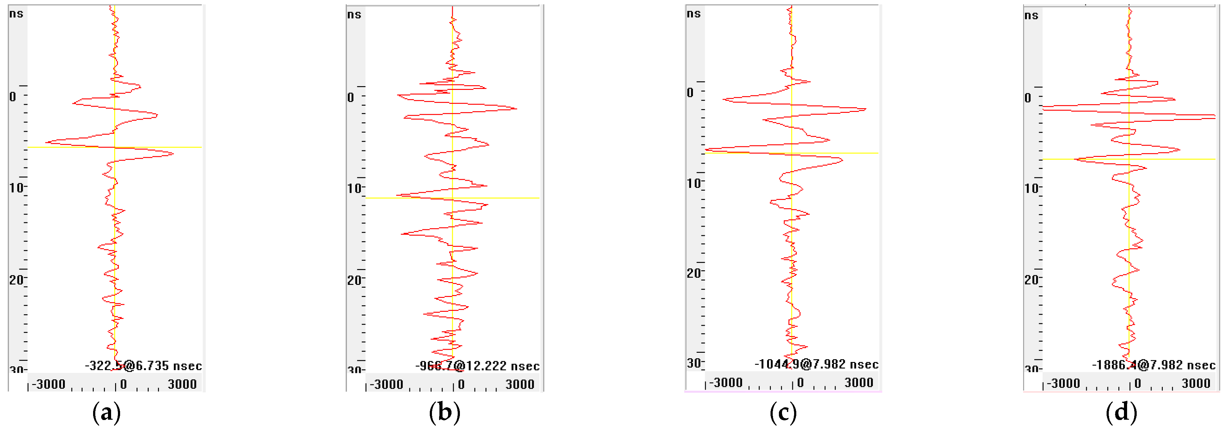
Figure 2 illustrates the A-scan waveforms for two cavities and non-cavities, such as loose gravel layers and buried pipes.
2.1.2. Images of B-Scan
The B-scan in the x-z domain is comprised based on various A-scan data along the scanning path (x-axis in
Figure 1). For the cavities selected by independent signal shapes in the A-scan plane image, a two-dimensional B-scan is generated, displaying longitudinal and cross-sectional images as shown in
Figure 3. After, in the B-scan, the signal strength, phase changes, and patterns of parabolic shapes are analyzed and verified. Typically, boundary surfaces reflecting the received signal are represented as curves or straight lines. The boundaries of underground objects or cavities appear in a parabolic shape. The upper point of a cavity is indicated by the topmost part of the parabola formed beneath the survey point, shown as white and black sections.
Additionally, A-scan and B-scan images can be used to determine whether an underground pipe is made of metal or PVC material. In the analysis of A-scan and B-scan images, if the start of the embedded image appears as (+) or white, it indicates a metallic material, such as a cast iron or steel pipe used for gas or water lines. Conversely, if the image appears as (-) or black, it indicates a PVC material, commonly used for communication conduits.
2.1.3. Images of C-Scan
Due to strong surface reflections, B-scan images often display dominant linear features that appear nearly straight. These surface reflections typically overwhelm underground reflections via the sudden change in permittivity from air (1 F/m−1) to paved road (5 F/m−1). These linear features in B-scan images can often interfere with the detection of underground objects. Therefore, B-scan images obtained using multiple antennas are combined to generate C-scan images that are visible in the x-y domain. The various C-scan images can be examined along the z-axis, representing depth, and these cross-sectional C-scan images are used to further characterize the detected features.
To analyze cavity signals, the changes in signals are examined three-dimensionally in the planar image, and shape changes with depth are confirmed. As shown in
Figure 4, buried pipelines exhibit a linear pattern, while cavities form a distinct area with abrupt amplitude changes along the boundary, showing an independently separated pattern. Therefore, cavities need to be identified by comprehensively analyzing planar, longitudinal, and cross-sectional images based on the independent signal shapes.
2.2. Background Filtering Algorithm (BFA)
In this study, a filtering algorithm of noise removal was developed to enhance the visibility of underground objects by removing dominant linear features and unwanted pattern noise from B-scan images. It is a background filtering algorithm (BFA). This algorithm consists of six steps. The filtered images can significantly enhance the visibility of underground cavities and are effectively used in the subsequent process involving the ResBlock technique applied to the C-GAN model. The workflow diagram for the BFA is illustrated in
Figure 5.
2.2.1. Collection of 3D GPR Data
3D GPR data are collected using multi-channel antennas to receive raw data from the underground space, as illustrated in
Figure 1. This setup allows for the acquisition of raw data corresponding to 25 channels, providing 25 longitudinal, planar, and cross-sectional views of the underground space. It is important to note that the measured GPR signals generally attenuate as they propagate through specific media. This attenuation must be considered during the data analysis process.
2.2.2. Conversion and Restructuring of Data
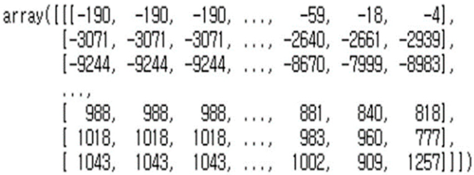
The raw data obtained from 3D GPR must be converted into a format that can be processed by deep learning models. The raw data are in an RD3 format, consisting of a combination of texts and numbers, and are not directly analyzable. Therefore, a decoding process was performed to convert these data into a one-dimensional array (1D-array) format, with numbers listed in a single column. This process utilized the Numpy library and involved converting the RD3 format raw data into the NPY format (*.npy). Subsequently, a data restructuring step was carried out to convert the one-dimensional array data in the NPY format into a three-dimensional array format, making them easier to use in deep learning applications. This conversion allows the data to be visualized and analyzed based on each antenna channel, the depth of the underground space, and the distance between the antenna and the underground cross-section.
As shown in
Figure 6, the reshape function of the Numpy library was used to reconstruct the one-dimensional array data into three-dimensional array data. The three-dimensional array data consist of elements arranged as follows:
[Antenna Channels (width of the survey vehicle)]
[Depth of the Underground Space]
[Distance between the Antenna and the Underground Cross-Section (distance along the survey vehicle’s driving direction)]
Etc.
2.2.3. Alignment of Data
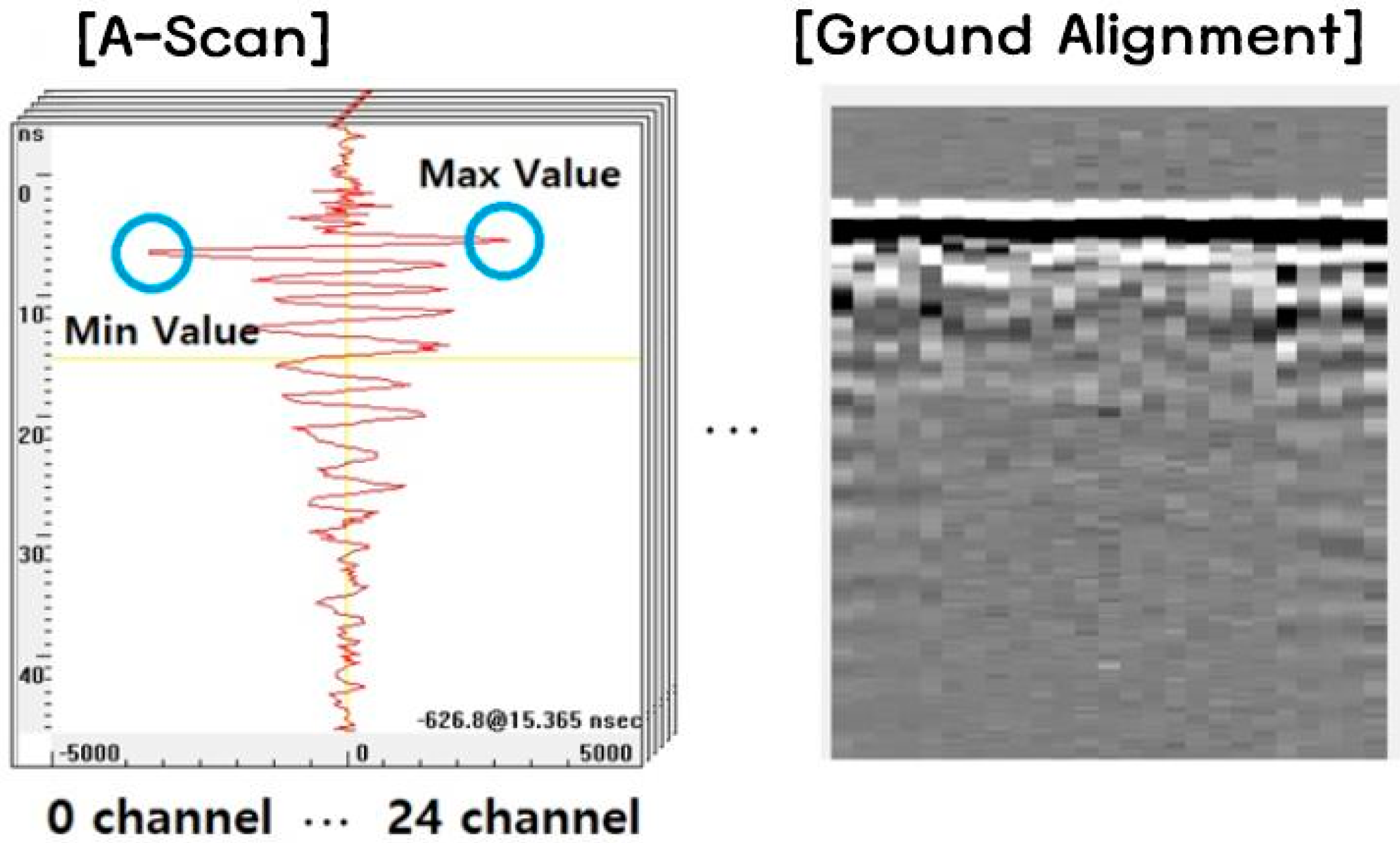
A ground alignment process is performed to correct the time differences using the maximum and minimum values of the data for each channel. In the case of a 3D GPR, the reflected waves received by the antenna with 25 channels are not received at exactly the same time, so they need to be aligned by tracking the ground surface. Specifically, as shown in
Figure 7, the first alignment value is calculated as the average of the maximum and minimum values of the data for each channel, and the second alignment value is calculated as the median of the maximum and minimum values of the data for each channel. By considering the pixel point corresponding to the average of the first and second alignment values as the ground surface corresponding to the underground space, the time difference for each channel can be corrected based on this pixel point.
2.2.4. Background Removal and Data Interpolation
The surface portion of the data, which has undergone the data alignment process, generates strong signals unrelated to cavity signals, interfering with the detection of cavity signals. Additionally, some channels occur bias. Therefore, noise in the surface portion must be removed and bias values adjusted by subtracting the average pixel values at specific depths in the underground space. This process is known as background removal. Subsequently, data interpolation is performed. This step ensures that the data structure and format of the pre-processed data match those of the training data used for the deep learning model. The intervals between pixels in the data are adjusted to a set value.
2.2.5. Data Amplification
When the transmitted waves from the antenna pass through the boundaries of different media, reflected waves occur based on the reflectivity of the media, and only the transmitted waves continue. As the depth of the underground space increases, the strength of the transmitted waves weakens, and the strength of the reflected waves also diminishes. Consequently, signals below a specific depth become difficult to observe during the process of visualizing and analyzing the data. Previously, signal amplification was performed using linear functions or exponential functions, but this approach often resulted in excessive noise.
Therefore, this study aims to achieve an optimal data amplification appropriate for different depths in the underground space by varying the degree of amplification for the relatively shallow and relatively deep parts of the data. Specifically, a signal amplification filter, represented by a function (
erf), is applied to the data to dynamically adjust the amplification weights for different depth intervals: the shallowest part (Zone 1), a deeper part than Zone 1 (Zone 2), and a deeper part than Zone 2 (Zone 3). The amplification filter function (
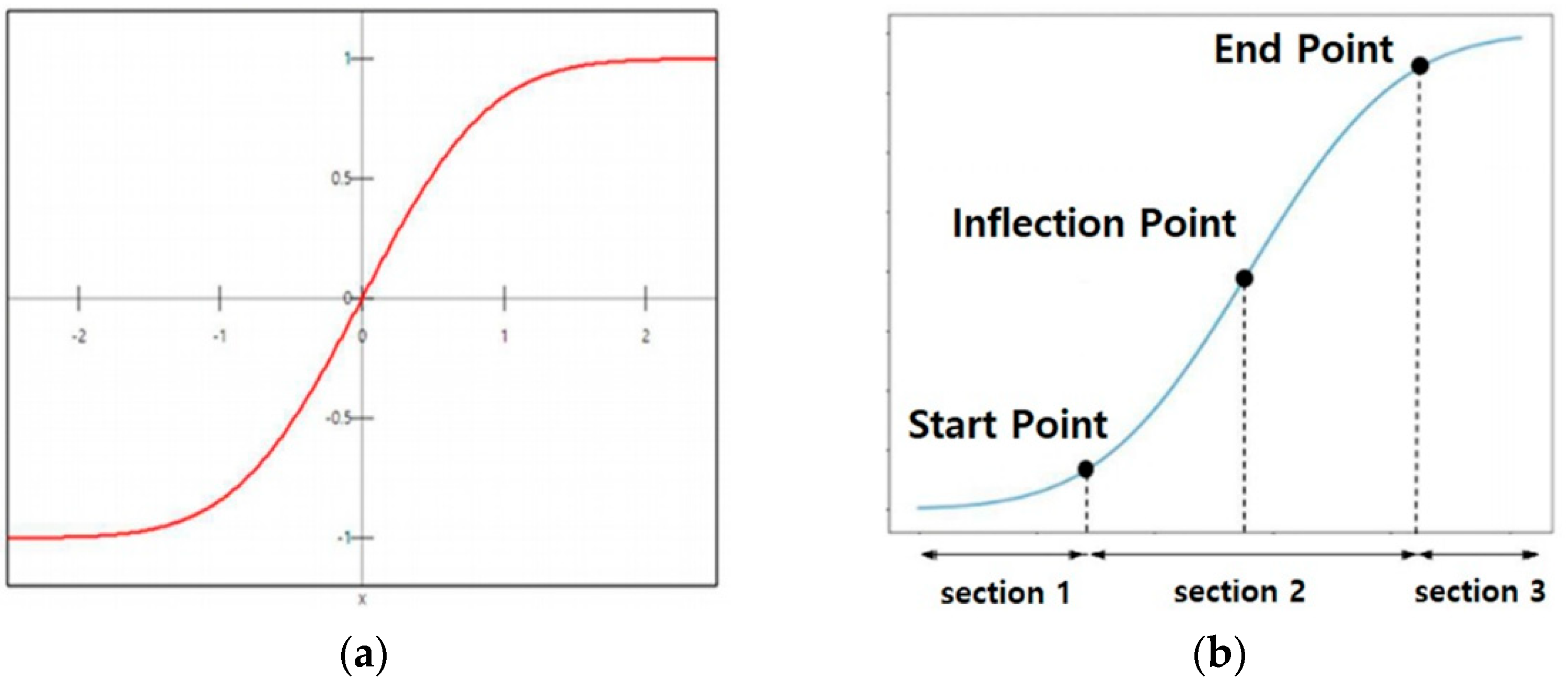
erf) is a Sigmoid error function, as shown in Equation (1) and
Figure 8a.
When applying this error function directly to amplify data with underground depth, it proved difficult to accurately detect cavities due to mismatches with the depths, widths, and sizes where cavities occur. Therefore, the error function was improved to create a new function (F), and this signal amplification filter was applied to amplify the data. Specifically, based on the error function expressed in Equation (1), additional variables were set, including the inflection range (the width between the start and end points of the inflection), the inflection midpoint (the midpoint between the start and end points), the slope of the function (erf) within the inflection range, and the y-axis intercept (bias) of the function (erf).
The final corrected error function (
F) can be expressed as shown in Equation (2).
Figure 8b illustrates the graph of the improved signal amplification filter function (
F) based on Equation (2). Here,
F represents the function of the signal amplification filter,
x denotes the pixel value according to the depth of the underground space,
a is the inflection midpoint (=140),
b is the inflection range (=70),
K is the slope of the function (
F) within the inflection range (=1),
C is the y-axis intercept (bias) of the function (
F) (=1.5), and
t is time. The x-axis represents the pixel values according to the depth of the underground space, which can be in units of pixels or cm. The y-axis represents the weight for the degree of data amplification. Additionally, the default values may vary depending on the characteristics of the underground space.
Figure 9 shows the data images before and after the application of the signal amplification filter. When the signal amplification filter is applied, it is evident that the data near the cavities are relatively more prominently amplified. This indicates that the applied improved error correction function is appropriate.
2.2.6. Noise Removal Using Local Average Subtraction
In data where errors have been corrected using traditional Kalman filters, signals that appear as straight lines in the direction of the survey vehicle’s travel (e.g., pipe signals, surface signals) are not effectively removed. As a result, these straight-line signals frequently overlap with the signals from the cavity regions. This means that the cavity signals are obscured by the straight-line signals in the direction of travel.
In this study, a Gaussian function was used to remove noise in the direction of the survey vehicle’s travel. However, applying a typical Gaussian filter would remove not only the noise but also the signals from the cavity regions. Therefore, in this study, instead of directly applying the Gaussian filter, a method is used in which the operation value of the Gaussian function is subtracted from the pixel value of the target pixel. This helps to selectively remove only the noise according to the driving direction of the survey vehicle.
The C-GAN model is considered the most suitable model for ground cavity prediction. The traditional deep learning method of a CNN (convolutional neural network) was initially used to extract image features for ground cavity detection. A total of 1396 image files were created and applied for training the CNN model, and 236 images were prepared for testing, resulting in an accuracy rate of 80.2%. In comparison to the C-GAN model, which achieved a 100% accuracy rate, the CNN model failed to reflect the entire dataset. Thus, the suitability of the C-GAN model for prediction after ground cavity detection was confirmed.
Figure 10 shows the data images before and after removing the straight-line noise in the direction of travel using local average subtraction. It is evident that noise near the surface and in the direction of travel, such as from pipes, is significantly reduced. Specifically, pixel values within a defined range centered on the direction of travel are selected, and the calculated value of the Gaussian function
G(
x), expressed by Equation (3), is obtained based on the central pixel value xxx within the defined range. By subtracting this calculated value
G(
x) from the pixel value (
x), noise in the direction of travel can be removed. Here,
σ is a predefined standard deviation value.
2.3. C-GAN-Based Automated Underground Cavity Detection
By inputting preprocessed data into the deep learning model, it is possible to predict cavities within underground spaces. The deep learning model used in this study is a C-GAN (conditional generative adversarial network), which is an improved form of the traditional GAN. In a GAN, a generator and a discriminator compete during training, but in C-GAN, conditional data are input to obtain the desired images. There are two representative types of C-GANs: pix2pix and cycle GAN. This study uses pix2pix, which, unlike traditional GANs, inputs images instead of noise for training, and the generator learns to produce images as a result. To enhance image generation performance, the model structure employs a U-Net form, incorporating the residual block technique with skip connections to prevent vanishing gradients.
Figure 11 illustrates the data processing flow of the deep learning model utilized in this study.
Figure 12 depicts the C-GAN architecture that can output cavity sections within the underground space based on pre-processed input data and pre-trained training data from 3D GPR data. Using this model eliminates the need for the reliance on expert concentration or subjective judgment in cavity surveys, allowing for real-time cavity detection and a rapid response to sudden road subsidence incidents. The predicted cavity sections in the deep learning model can be adjusted to display as images highlighted with specific colors.
3. Field Validation Tests
The deep-learning-based underground cavity automatic detection technique derived in the previous section was applied to the roads in Seoul, Republic of Korea. The validity of this technique was verified using the collected 3D GPR data.
3.1. Experimental Setup
Figure 13 shows the vehicle-type multi-channel GPR used in this field investigation. The GPR has a frequency of 400 MHz, and its effective investigation depth and width are up to 2.0 m from the surface of flexible pavement and 2.4 m, respectively. Moreover, the multi-channel GPR can perform 3-dimensional analysis; therefore, it can detect the interface of different materials and abnormal signals owing to the differences in the relative permittivity, even in identical materials. The GPR system comprises GPR antennas, a camera recording surface conditions, a global positioning system (GPS), and positioning cameras [
16].
This system consists of 14 transmitting antennas and 14 receiving antennas, totaling 25 channels, and extends the survey width to 2.4 m, allowing data acquisition without survey shadow areas in a single pass. Additionally, the vehicle-based GPR survey software is divided into software for recording and controlling in the field and software for analyzing and recording data indoors. In the field, MIRA Software v.3.57.01 from MALA was used to record and control the survey equipment. For survey data analysis, a combination of MALA’s rSlicer v1.0.0 and the GPRIS System developed in the Republic of Korea was utilized.
Figure 14a shows the radargram of a cross-section in the longitudinal direction from the GPR scanning, and the yellow circle represents that an underground cavity may exist. The horizontal axis indicates the distance in the longitudinal direction, and the vertical axis indicates the depth from the pavement surface. The depth from the top surface to the center of the parabolic black strip is defined as an overburden thickness measured as 0.33 m in this study. To determine the size of the cavity from the image, the boundary of the white strip above the black parabola that indicated an amplitude change in the GPR signal was set as the boundary of the cavity, and the length between the boundaries was defined as the size of the cavity.
Figure 14b shows the radargram of a planar image at a depth of 0.67 m that represents the overburden thickness of the cavity.
The data in
Figure 14a are non-migration data. The objective of this study is not to determine the size of the cavities but to evaluate the performance of cavity pre-processing using the BFA, making migration unnecessary in this context. Of course, during data acquisition, the apparent structure (hyperbola) reflected in the images is converted into the actual underground structure using correction methods to measure the scale of the cavity. Migration is typically used to reposition inclined surfaces to their actual underground locations and to reduce diffractions. According to the literature [
16], approximately 70% of cavity waveforms detected through GPR surveys are considered to represent the actual size of the cavity, allowing for an approximate estimation of its size. However, as previously mentioned, migration is not a mandatory requirement for this study, so it was not performed.
3.2. Results of Appling the BFA
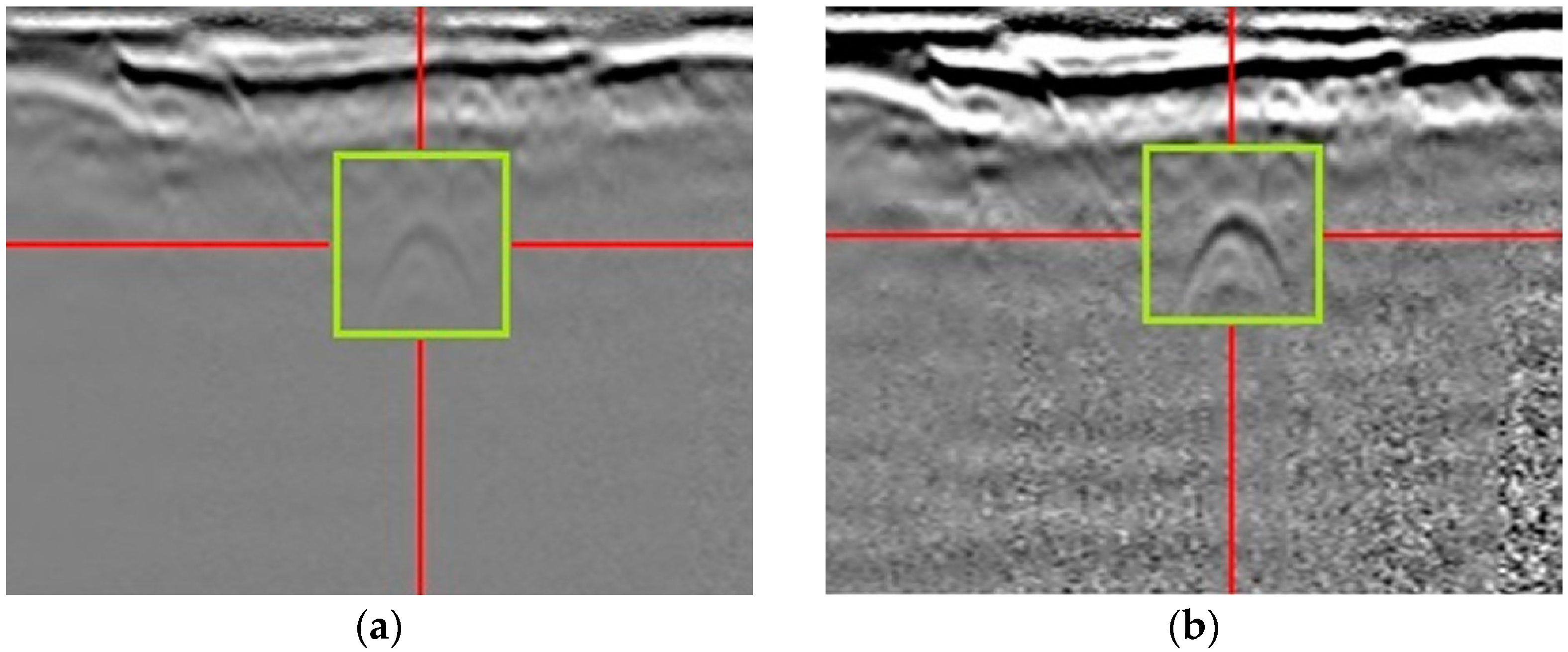
Figure 14 shows the longitudinal and cross-sectional views at locations with cavities, comparing images detected with and without the application of the BFA. In the longitudinal section, as shown in
Figure 15a, the cavity appears in the form of a curve known as a parabola or hyperbola. In the upper image of
Figure 15a, where the BFA is not applied, the boundary feature information of the target (underground cavity) has a weak intensity, and the geometric structure of the hyperbola is not distinct. However, in the lower image of
Figure 15a, where the BFA is applied, signals that appear as black and white bands, indicating the boundary characteristics of the asphalt pavement and soil medium near the surface, are removed, making the features of the underground cavity in the longitudinal section more clearly identifiable.
Similarly, the underground cavity in the cross-sectional view shown in
Figure 15b also exhibits the characteristic parabolic or hyperbola curve shape. In the image on the right side of
Figure 15b, where the BFA is applied, the black and white bands near the surface are removed, making the boundary of the cavity’s curved shape more prominently defined.
Figure 16 shows the plan view (C-scan) at locations with cavities, comparing images with and without the application of the BFA. When examining the plan view at the same depth, it is observed that the local area is represented in black before the BFA is applied. In contrast, after applying the BFA, the black areas in the image are clearly distinguishable as underground cavities, confirming the effectiveness of the BFA in enhancing the visibility of these features.
Figure 17 and
Figure 18 present the analysis of underground cavity images at specific depths in the plan view, comparing cases with and without the application of the BFA. The data with the BFA applied, obtained at 3 cm depth intervals, showed a reduced influence from surrounding signals at all depths. As a result, the closed-loop boundaries characteristic of the underground cavities in the plan view became more distinct, and independent region images were formed more clearly.
Figure 19 and
Figure 20 show the images of data from five channels where the parabolic shape characteristic of cavities in the longitudinal section is well-visible. These images compare the data without the BFA applied and with the BFA applied. In the five channels, the data without the BFA areis obscured by the black and white straight-line signals representing the boundary characteristics of the asphalt pavement and soil medium. In contrast, the data with the BFA applied clearly show the upper and lower boundary characteristics of the parabolic cavity shape in the longitudinal section, demonstrating that the cavity features are more distinctly detected.
3.3. Verification of the BFA Effect Using the Pre-Trained C-GAN Model
The 3D GPR data used in the C-GAN model include a total of 12 cavities, with 25 channels, a depth of 2.5 m, and a survey distance of 6215 m. To verify the effect of applying the BFA, tests were conducted and analyzed in two cases: without the BFA and with the BFA applied. Each dataset was input into the pre-trained C-GAN, and it took approximately 22 min to analyze a total distance of 12.4 km.
Assuming the analysis depth is around 80 cm, the 3D GPR data can be viewed as a rectangular prism with dimensions of 25 channels × 0.8 m (depth) × 6215 m (distance). Dividing this rectangular prism into smaller prisms of 5 channels × 0.4 m (depth) × 1 m (distance) results in 62,150 smaller rectangular prisms. The classification results of these 62,150 prisms, when using a confusion matrix, are shown in
Figure 21. The x-axis represents the actual values, and the y-axis represents the predicted values. In detail, in the actual value, T is True (Cavity), and F is False (Non-Cavity), while in the predicted value, P is positive (Cavity), and N is Negative (Non-Cavity).
Thus, TP and FN indicate the accuracy of the C-GAN model, while TN or FP indicates the prediction failures by the C-GAN model. As an effect of applying BFA, TP and FN increased slightly, but these values are negligible compared to the overall data.
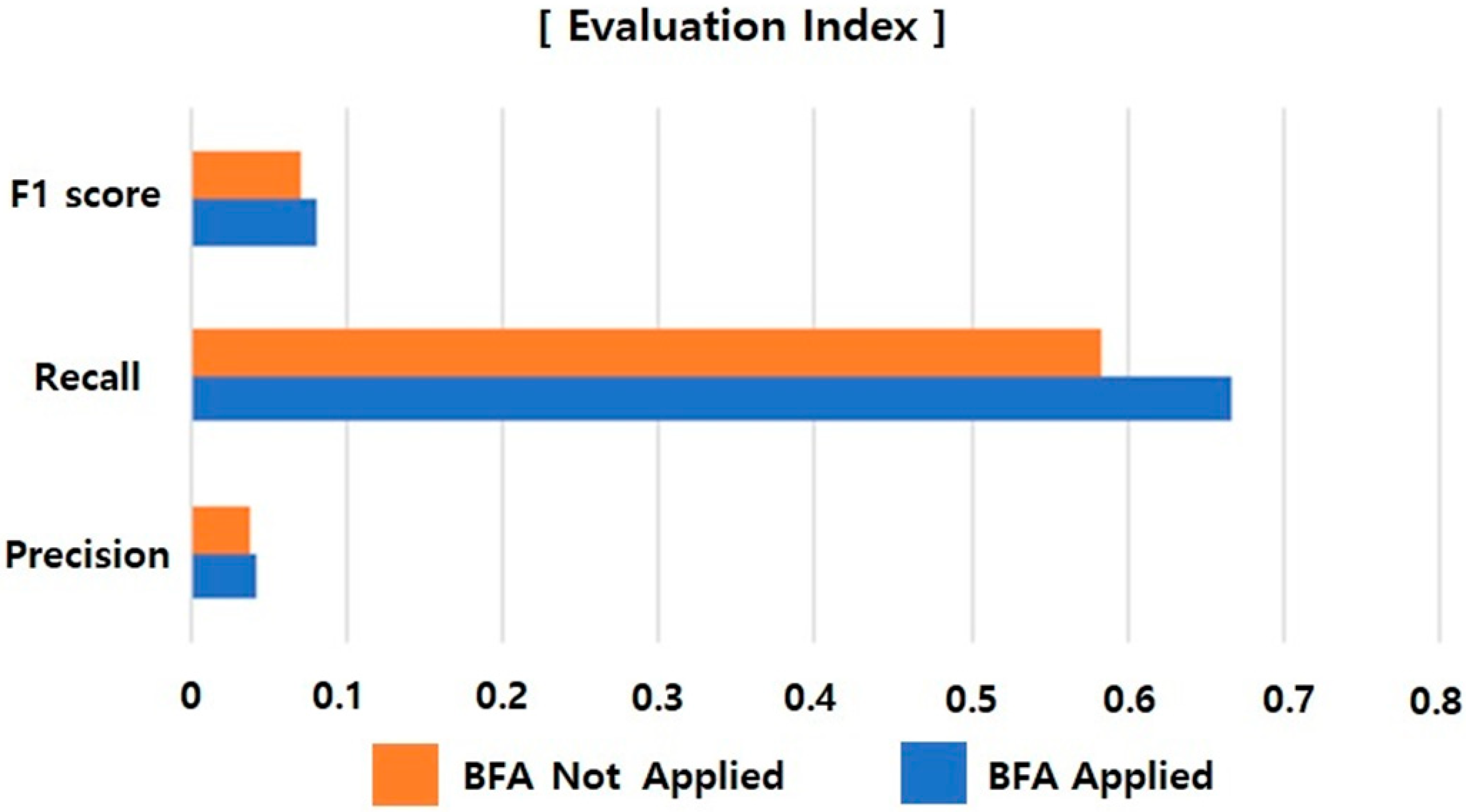
To quantitatively analyze the accuracy of the underground cavity detection results, a comprehensive evaluation index (
F1 Score) for the fitted characteristic hyperbola was used. This can be calculated as shown in Equations (4)–(6). Here,
P is precision, and
R is recall. TP, FP, and FN represent true positives, false positives, and false negatives.
Figure 22 shows the results of the model classification applied to Equations (4)–(6). These results illustrate the impact of the proposed BFA technique on performance through three indicators: F1 score, Precision, and Recall. The high value of false positives affects the F1 score and Precision, resulting in generally some lower values for these metrics. However, both metrics showed higher values when the BFA was applied. Additionally, in a cavity survey, the most crucial aspect is ensuring safety by accurately detecting all cavities. Therefore, Recall, the indicator of how well the C-GAN model predicts actual cavities, is vital. Comparing the Recall values with and without the BFA application, the model with the BFA applied showed higher Recall values by about 15%.

