Abstract
Integrating coastal topographic and bathymetric data for creating regional seamless topobathymetric digital elevation models of the land/water interface presents a complex challenge due to the spatial and temporal gaps in data acquisitions. The Coastal National Elevation Database (CoNED) Applications Project develops topographic (land elevation) and bathymetric (water depth) regional scale digital elevation models by integrating multiple sourced disparate topographic and bathymetric data models. These integrated regional models are broadly used in coastal and climate science applications, such as sediment transport, storm impact, and sea-level rise modeling. However, CoNED’s current integration method does not address the occurrence of measurable vertical discrepancies between adjacent near-shore topographic and bathymetric data sources, which often create artificial barriers and sinks along their intersections. To tackle this issue, the CoNED project has developed an additional step in its integration process that collectively assesses the input data to define how to transition between these disparate datasets. This new step defines two zones: a micro blending zone for near-shore transitions and a macro blending zone for the transition between high-resolution (3 m or less) to moderate-resolution (between 3 m and 10 m) bathymetric datasets. These zones and input data sources are reduced to a multidimensional array of zeros and ones. This array is compiled into a 16-bit integer representing a vertical assessment for each pixel. This assessed value provides the means for dynamic pixel-level blending between disparate datasets by leveraging the 16-bit binary notation. Sample site RMSE assessments demonstrate improved accuracy, with values decreasing from 0.203–0.241 using the previous method to 0.126–0.147 using the new method. This paper introduces CoNED’s unique approach of using binary code to improve the integration of coastal topobathymetric data.
1. Introduction
The importance of consistently integrated topobathymetric data has been well documented for over 20 years [1]. This significance was demonstrated with the release of the first regional-scale seamless multisource topographic and bathymetric elevation model for Tampa Bay, Florida, through a partnership between the U.S. Geological Survey (USGS) and the National Oceanic and Atmospheric Administration (NOAA) in 2001 [2]. This partnership paved the way for integrating topographic and bathymetric data into a unified spatial reference at larger scales, broadening the scope for regionalized coastal research. Recognizing this need for regional topobathymetric models, in 2011, the USGS formalized the Coastal National Elevation Database (CoNED) Applications Project focusing on the research and development of seamless, integrated topobathymetric elevation models (TBDEMs) derived from multiple topographic and bathymetric sources. Following a research period, CoNED published the topobathymetric elevation modeling method (TEMM), which describes integrating disparate data sources to create regional TBDEMs [3]. Since this publication, the project has published 12 regional TBDEMs averaging 40,000 km2 by applying this method, covering around 60% of the conterminous U.S. coastline at a 1 m spatial resolution (Figure 1).
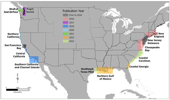
Figure 1.
Spatial extent of Coastal National Elevation Database’s (CoNED’s) regional topobathymetric model (TBDEM) products for the conterminous United States (CONUS) averaging 40,000 km2. Each data series is color-coded, representing its publication year, with 12 published between 2016 and 2023.
Over this period, the techniques for acquiring topobathymetric and bathymetric data have continued to diversify using varying sensor types and collection methods [1,4]. This diversification has offered improved accuracy, increased spatial density, and provided more complete spatial coverage by the increased use of platforms such as uncrewed aircraft systems (UASs) and remotely operated vehicles (ROVs) [1]. These new methods have improved the reach for collecting bathymetric data, from the quick deployment of UAS for rapid response to ROV accessing shallow hazardous to deep waters. These collection methods, along with traditional airborne topobathymetric light detection and ranging (lidar) and the adoption of data blending methods such as the fusion approach described by Petrasova et al. [5], can extend the use of high-resolution topobathymetric elevation models for localized modeling. Although improved accuracy and current data are the desired elements for modeling coastal environments, assembling large regional models requires a broader range of temporal and spatial resolution source data to develop continuous elevation models. These large composite models composed of a broader spectrum of input sources can reveal substantial variability along the seamline of the adjacent source elevation models. The TEMM published in 2016 addresses fundamental spatial differences such as horizontal and vertical datum transformation and geoid vertical alignment but does not address the mitigation of substantial vertical discrepancies between adjacent data in the nearshore and bathymetric domains [3]. These disparities often create artificial barriers, slope creep artifacts, and sinks along the intersections of neighboring datasets. These boundary issues are problematic in modeling environments that use the elevation surface to model wave action, inundation, tidal flows, and sediment transport (Figure 2).
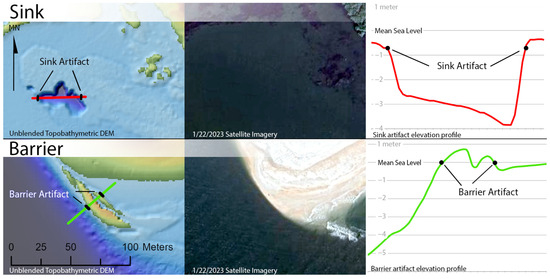
Figure 2.
The top half highlights an example of an artificial sink that occurs when high-resolution topobathymetric data are merged with coarser interpolated sonar records. The missing topobathymetric data are typically a result of poor water clarity, resulting in invalid lidar returns. The red line is a cross section of the sink with its elevation profile to the top right half. The bottom half highlights an example of an artificial barrier that occurs when older topographic elevation exposes areas of shoreline recession. These also typically occur when there are voids in the topobathymetric data, exposing the older topographic data that has receded. The green line is a cross section of the barrier artifact, and to the far right is its elevation profile—satellite imagery credit to Google and Airbus.
The blending or merging of adjacent datasets, often referred to as fusion, is applied at different levels of complexity based on the context of the datasets that are being blended. Blending can be a simple linear weighted average over a fixed width of overlap or more complex by applying a variable width blending as described by Petrasova et al. [5] to a contextual-based adaptive-weighted multi-resolution regularized framework described by Fuss et al. [6] and Yue et al. [7]. Moreover, in recent years, there has been an investigation into applying artificial neural networks (ANNs) blending high-resolution datasets with low-resolution datasets like Shuttle Radar Topography Mission (SRTM) to improve the overall accuracy of the lower-resolution datasets, showing promise to help improve lower-resolution bathymetric data [8,9].
These blending approaches each have elements to enhance the TBDEM where data overlap potentially exists. CoNED is confronted with data integration challenges before these enhancements can be realized. First, the blended data typically fall near and in coastal tidal zones, where the surfaces continuously change due to the constant energy flow, making continuous blended surfaces from varying acquisition excessively burdensome [10]. Second, CoNED data integration does not consistently blend high-resolution data but equally blends high-resolution topobathymetric data with moderate- to low-resolution bathymetric datasets with a lack of consistent accuracy assessment due to the limited number of control measurements [11,12]. This lack of controlled measurements minimizes the confidence in expending additional resources required to implement a complex blending method because of the varying and unknown levels of uncertainty in the bathymetric domain. Compounding these challenges is that the CoNED project typically develops TBDEMs with an average area of 40,000 km2. Therefore, producing more complex models at this scale affects the resources needed to create these large composite models.
As a result of these challenges with the data, CoNED chose to use modified linear weighting methods to mitigate these vertical differences between neighboring datasets. The method developed introduced a variable-weight linear blending step in the TEMM’s integration component that collectively assesses the input elevation models to define how to transition between disparate datasets (Figure 3). The new step defines two transition zones. The first transition zone, or micro blending zone (MiBZ), occurs along the coastlines, specifically the interface between 1 m, high-resolution, topographic digital elevation models (DEMs) above mean sea level (MSL) and the adjacent bathymetric DEMs (Figure 4, red inset). The second transition zone, or macro blending zone (MaBZ), occurs when a high-resolution, bathymetric DEM overlaps moderate- to low-resolution (greater than 10 m) bathymetry (Figure 4, green inset).

Figure 3.
(A) is the topobathymetric elevation model method (TEMM) integration workflow [3]. (B) highlights where the new micro/macro blending is added in the TEMM integration workflow.
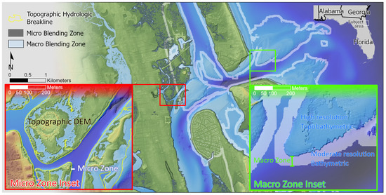
Figure 4.
A map of the St. Augustine, Florida, coast illustrating the locations of the macro blending zone (MiBZ) [black] and macro blending zone (MaBZ) [white] transition zones. The red inset map shows the MiBZ and includes hydrologic breaklines (yellow lines) defined by the high-resolution topographic digital elevation models (DEMs). The green inset map is at the same scale as the MiBZ inset but highlights the typical location and a wider MaBZ.
Because CoNED aims to provide the best available data for its regional TBDEMs, this additional blending step limits the alteration of edge pixels in these zones by analyzing all the inputs for a pixel to determine whether blending is required or what input pixel value should be used. A multidimensional classification schema was developed using binary notation to achieve this analysis on a regional scale. The binary notation method can efficiently evaluate all the inputs based on quality and temporal acquisition at the pixel level to identify the blending method of adjacent datasets in each zone. A general workflow diagram of the method is shown in Appendix A; the workflow (WF) steps are referenced in the text by bracket “[WF-step number]” notations.
2. Methods
To create the micro and macro blending zones, a multidimensional array is generated that classifies the elevation state of the input datasets at the pixel level. The array is then used to determine whether an existing dataset’s value is applied or if interpolation is necessary, and how best to apply the interpolation. The following sections go through quantifying the input data, determining if interpolation is required, selecting the appropriate method, creating MiBZ and MaBZ elevation models, and applying it to the final integrated TBDEM.
2.1. Creating a Quantitative Value—The Bit-Pack
All the input data are prioritized to generate a quantitative value for each pixel, as stated in TEMM’s integration component step 5. These overall priority values are based on the accuracy and acquisition date of an input dataset; the higher quality and more current datasets are given the higher priority [3]. It is worth noting that data with close priority values can have the same or similar quality assessments and acquisition dates, but one may be rated higher than another. In situations like this, these data typically have minimal or no spatial overlap, highlighting that priority ratings represent the broader data collection and do not reflect the quality of the adjacent prioritized dataset. Once prioritized, the source data are then grouped into five hierarchical categories based on the elevation characteristics shown in Table 1 [WF-3] (seven categories are listed, and two are labeled open for potential new dataset integration).

Table 1.
Hierarchical elevation categories and descriptions. Notice that CAT03 and CAT07 are referred to as open and serve two purposes: first, they are required to complete a 16-bit integer binary code, and second, they are placeholders for additional inputs.
Each category is then composited into a single mosaicked DEM that is stacked based on the overall priorities where the higher priority data supersede the lower priorities. It is important to note that it is valid for a category DEM to have no data pixel values [WF-4] (Figure 5). To create quantitative values, a 16-layer binary dataset is derived from the five composite category DEMs. These binary layers are composed of the blending zones [WF-6] and fourteen binary layers derived from the seven composite DEMs in Table 1 [WF-7]. The first two binary layers represent the micro and macro blending zones, where a pixel value of 1 indicates it is inside the respective blending zone, and a 0 indicates a pixel falling outside a zone [WF-8]. The remaining fourteen layers are referred to as binary pairs because two binary layers are created from each category composite DEM. These binary pairs assess the category’s vertical status for each pixel.
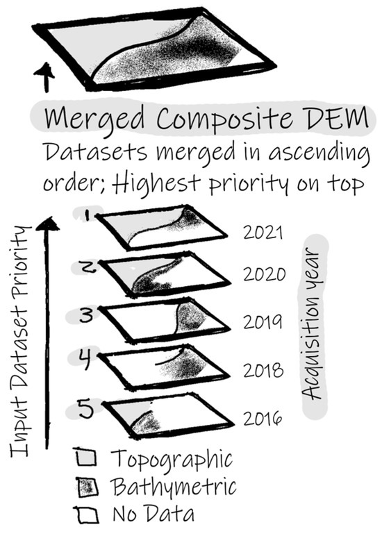
Figure 5.
In the illustration, five datasets are grouped in the topobathymetric category (CAT02) assigned priorities one through five. The stacking order is in descending order with priority five on the bottom and one at the top. The solid gray color indicates land, the speckled black is bathymetric elevations, and the white indicates no data. The final composite DEM is made of primarily the 2021 priority one dataset, but where no data exist, the lower priority data are used to fill the no-data spaces in succession. Priority five dataset is not applied in the composite because the higher priority datasets cover that layer with data. The composite still has some no-data space in the lower right corner because none of the input sources had valid elevation data seen in panel B.
The binary pair describes where there is valid data and the vertical position of that valid data relative to MSL as defined by the North American Vertical Datum of 1988 (NAVD88) (Figure 6). The first layer in the pair represents the existence of elevation data, indicated by a value of 1 and a 0 for no data (Figure 6B). The second layer in the pair represents a pixel’s relative position to MSL; a 1 indicates a pixel’s value at or below MSL, and a 0 represents values above MSL (Figure 6C). The two open categories, CAT03 and CAT07, referenced in Table 1 have binary pairs composed of all the 0-pixel values to provide a total of 16 binary layers. These 16 binary layers are then stacked in a defined sequence to create a multidimensional array (Figure 7, Step 1). These layers along the Z-axis render a 16-bit binary code for each pixel. This code is compiled into its respective integer value and transformed back to a two-dimensional (2D) geospatial dataset, with the appropriate spatial reference system applied (Figure 7, Step 2). The resulting dataset is referred to as the Bit-pack and is used to drive the blending algorithm by leveraging an integer’s inherent binary code as a pseudo-lookup table. The binary code is an effective method for evaluating each pixel to determine whether it requires interpolation or the insertion of an existing elevation source based on the sequence of ones and zeros.
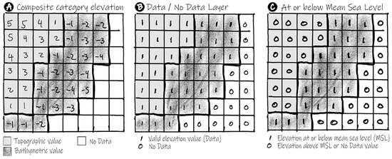
Figure 6.
Binary pair created from a category composite digital elevation model (DEM). Panel (A) illustrates pixel values in a composite DEM, where the blank squares (pixels) represent no data. Panel (B) illustrates the binary classification for the data/no-data binary layer, where a 1 represents pixels with valid elevation and a 0 represents pixels with no data. Panel (C) illustrates the binary classification of elevations below or above mean sea level (MSL), where a 1 represents a pixel at or below MSL and a 0 represents both pixels above MSL and no-data pixels. Together panels (B,C) represent a binary Pair.

Figure 7.
Three steps in converting 16 binary layers into a single band 16-bit integer Bit-pack geospatial data layer. Step 1 is stacking the 16 binary layers based on priority into a single 16-band data array. Step 2 is compiling the 16-band data array into a 2D 16-bit integer array that represents each pixel’s z-axis binary code. Step 3 is converting the 2D array into a geospatial readable raster format with appropriate geospatial positioning.
To illustrate this binary approach, Figure 8 shows a simplified example of three conditions in a Bit-pack dataset and how they are used to identify an area for interpolation. Panel A in the figure shows the elevation datasets merged in order of priority absent any blending. The resulting prioritization inserted a shoreline artifact that has since receded between data acquisitions. This shoreline has receded and is confirmed by the 2022 imagery.
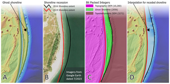
Figure 8.
Illustration of the removal of a receded shoreline. Panel (A) shows the ghost shoreline artifact. Panel (B) confirms the recession of the shoreline. Panel (C) is the resulting Bit-pack dataset indicating interpolation in the green area. Panel (D) is the result of an algorithm applying the information from Bit-pack results to create an improved representation of near-shore bathymetry. The red line indicates the topographic best available shoreline, and the black line represents the prior shoreline based on an earlier surface data acquisition. This example is east of the Cape Canaveral Launch Complex 46.
Panel C shows three quantitative values resulting from Bit-packing; the purple shade (value 10,280) indicates where the high-priority topobathymetric DEMs are used, and the green shade (value 2056) indicates the area of a receding shoreline where the bathymetric data require interoperation. Panel D shows the composite elevation dataset with the interpolation applied to the area where the shoreline has receded. The following sections detail how the binary code is used to collectively characterize all the input data for a given area, and how the characterization drives when a pixel is interpolated and the method of interpolation.
2.2. Interpreting the Binary Code
The Bit-packing method efficiently identifies the pixels that require interpolation to generate a continuous transition between disparate elevation sources. These blending zones are introduced into the TBDEMs to minimize the influence of artificial barriers and sinks by simulating logical transitions between the temporal and spatial disparate data sources.
The first step to implementing Bit-packing is to explicitly define how each binary layer is derived and its position in the multiterminal array or binary stack [WF-2] (Figure 7, Step 1). Figure 6 defines these binary layers and respective bits for the TEMM implementation. Each position in the binary code has an intrinsic value exponentially increasing from right to left [13]. With that intrinsic value, the binary stack should be prioritized, positioning layers with increasing importance from right to left. Having the layers sequenced from high to low preference generates inherent weight to the Bit-pack pixel value. Algorithms can then leverage these weighted values to query information efficiently and, in the TEMM, differentiate between the high- and low-value inputs to isolate the pixels that require further evaluation for interpolation.
As discussed earlier, the TEMM uses the micro/macro blending zone layers and the seven composite DEMs to create the Bit-pack dataset that drives the blending algorithm in these zones. The algorithm leverages an integer’s inherent binary code or sequence of “1”s and “0”s to determine if or how a pixel is interpolated. For a given pixel, the Bit-pack encodes the series 16 binary rasters to a single classification. This encoding is illustrated in Figure 9, showing how a Bit-pack integer value is interpreted by unpacking 48,184 into its respective 16-bit binary code. Moving left to right in the figure reveals all the binary layers for a given pixel, with the first two positions (15 and 14) indicating that this pixel falls in an MiBZ and outside an MaBZ (Figure 9). The following positions (13-0) indicate the elevation state of each elevation category (Table 1) based on the binary pair assessment in order of the categories’ hierarchical structure. A similar three-dimensional spatial representation is shown in Figure 10, which illustrates the stack of 16 binary arrays (layers), each representing a position in the binary code and the top layer representing the compiled 16-bit binary integer layer. The vertical lines transcending through the pixel array intersect the pixel that, when compiled, equals 48,184.
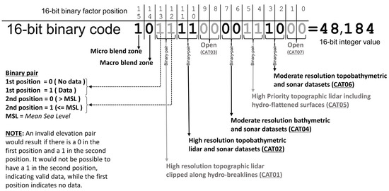
Figure 9.
Illustration of a 16-bit binary code. The smaller text on top indicates the position of the binary code from left to right. The larger 1s and 0s are the binary switches that compose a 16-bit binary integer. To the right of the equal sign is the integer value that the sequence of 1s and 0s represents. The arrows point to the description of each position or pair of positions. As of publishing, the “Open” label under positions 9, 8, and 1, 0 are not being used for analysis but are available for future use.
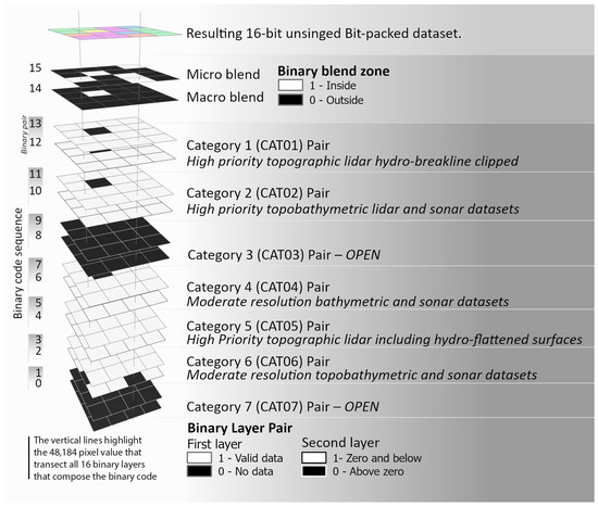
Figure 10.
The gridded squares represent a multidimensional spatial illustration of a binary stack. This stack of binary data layers represents the 16 layers to build the Bit-pack data layer noted at the top of the diagram in color. The description of each layer is to the right of the individual layer or layer pair. To the right of the binary stack is the position number that the layer is in the binary code. The two vertical lines transecting the binary stack highlight the two vertical stacks of pixels that, when compiled, represent the value 48,184.
A 16-bit pixel depth was selected because it is a standard bit depth providing direct implementation into a broad range of geospatial analysis software despite only having 12 binary inputs. As a result, four “Open” binary layers are introduced (Table 1) to complete the 16 input requirements. Instead of placing these open layers or positions at the front or end of the binary code, they are strategically placed at positions 9 and 8 as CAT03 and 1 and 0 as CAT07. These positions allow the inclusion of future binary layers with higher influential datasets in CAT03 and less significant inputs in CAT07 (Figure 9 and Figure 10).
2.3. Binary Position
The Bit-packing method is based on the properties of the binary code, treating the bit sequence as a lookup table to quantify each pixel. The resulting quantitative value represents the vertical state of all the pixels of each elevation category. The TEMM uses Bit-packing to identify possible input conflicts, including those inputs that result in sink and barrier artifacts and expose shoreline recession.
To explore the TEMM application of the binary code and its corresponding integer values, the value 48,184 is used as an example. Referencing Figure 9 as a guide, the binary code is examined from left to right. The first two bits indicate that this pixel is inside an MiBZ and does not intersect the MaBZ because position 15 is one and 14 is zero. Second, both the high-resolution topographic lidar (CAT01) and the high-resolution topobathymetric lidar and multi-sonar dataset (CAT02) have valid values as indicated by “11” in their respective binary pairs, with the first “1” representing valid data and the second “1” indicating elevation value below MSL. At this point along the binary code, there is enough information to assign an elevation value because the two highest-priority category pairs contain the necessary information to set an elevation value. However, this code sequence can provide more context to identify possible changes or indicated conflicts with the input data sources. Continuing down the binary code (ignoring positions 9, 8, and 1, 0 because these are open pairs), positions 7 and 6 represent a moderate-resolution bathymetric and sonar CAT04 binary pair. This pair indicates no data because the binary pair is “00”, with the first value being “0” indicating no data, and the second “0” must be zero because there cannot be a value if it is indicated to have no data. Positions 5 and 4 reference the hydro-flattened high-resolution topographic lidar (CAT05), and this pair is “11,” confirming the state of CAT01 because CAT05 includes the same datasets as CAT01 with the addition of hydro-flattened surfaces. Positions 3 and 2 are the moderate-resolution topographic, bathymetric, and sonar datasets. This pair value of “10” indicates valid data above MSL because the first value of “1” indicates valid data, and the second is a “0,” identifying elevation above MSL. From this sequence, a temporal observation could be made; with the recent data acquisitions from CAT01 and CAT02, the binary pairs indicate values at or below MSL, and the older acquired CAT06 binary pairs show values above MSL, indicating potential shoreline recession. If the Bit-pack value were 32,824 (binary code 10-00-00-00-00-11-10-00) where the CAT01 and CAT02 pixels do not cover this extent, indicated by the “00” in both pairs, a receded shoreline would be identified because the CAT05 pair “11” indicates a hydro-flattened value below MSL, and the CAT06 pair “10” indicates elevation above MSL and an interpolation would have been applied like what is illustrated in Figure 8, panel D. This interpretation of the binary code for 48,184 demonstrates how a well-designed binary input stack can offer multiple insights to assess a pixel.
The final step is identifying the appropriate dataset to extract the elevation value. In the prior TEMM integration, the high-priority dataset pixels would always supersede lower-priority datasets in spatial integration. With the introduction of the Bit-pack, each pixel can be evaluated to determine the appropriate input to insert into the respective pixel. Staying with the binary code for 48,184, this pixel has two high-resolution datasets with valid data, CAT01 and CAT02, and both are below MSL as indicated by their respective binary pairs (Figure 9). The CAT01 datasets use lidar near-infrared (NIR) and short-wave infrared (SWIR) wavelengths to collect land surface topography features, while the CAT02 datasets use a hybrid wavelength of NIR/SWIR and green laser at a 532 nm wavelength to penetrate water (surface and column) to acquire elevations (submerged topography) below the surface [14]. With the Bit-packed dataset steering the blending algorithm, any Bit-packed values of 48,184 will use the pixels from the CAT02 datasets in the integration process because they fall inside the MiBZ, and it has better fidelity when measuring bathymetry [14]. This logic can be extended further to query a range of values falling between 47,128 and 48,380 because their binary codes all indicate both the CAT01 and CAT02 datasets at or below zero falling inside the MiBZ (47,128 = “10 11 11 00 00 00 00 00”, 48,380 = “10 11 11 00 11 11 11 00”).
2.4. Data Prioritization
The prioritization of the input data, covered in the TEMM’s original publication, allows the TBDEM products to reflect the most accurate information [3]. Because the Bit-packing method was developed to mitigate elevation discrepancies between disparate adjacent datasets, it is pivotal to this discussion. However, data prioritization is not a requirement for implementing a Bit-packing method.
During the integration component’s initial stages, the TEMM prioritizes each topographic, topobathymetric, and bathymetric dataset based on its quality and acquisition date [3]. When applying the micro/macro blending method to the TEMM, additional steps are required for prioritization. When a topobathymetric dataset is given a higher priority than a CAT01 topographic dataset, the topobathymetric datasets must be identified twice in a priority list. One entry is linked to the topographic category (CAT01), and a second entry is linked to the topobathymetric category (CAT02). This separation allows the blending algorithm to isolate the topographic and bathymetric elevations where the topographic data are included in CAT01, and the bathymetric data are included in CAT02.
Prioritizing is an iterative process often involving the review of input source metadata and reports. Initially, setting priority is based on each dataset’s quality and acquisition date. This sequence is allowed to change if, after an evaluation of an interim version of the TBDEM composite, it is revealed that a given dataset is not suited for its initial priority level.
2.5. Dataset Categories
Categorizing datasets with common properties is not required for Bit-packing and is unnecessary when there are only a few binary input layers. The TEMM source datasets typically range from 30 to over 300, making it impossible to include all the individual datasets in the Bit-packing process. In cases where the input numbers are higher than 16, grouping common datasets may be necessary.
This blending method uses five hierarchical categories or collections of elevation datasets with common properties to derive the Bit-pack values; refer to Figure 10 for details on each category. These categories closely follow the priority set for each dataset; CAT01 includes the highest priority topographic datasets and can include topobathymetric data, CAT02 includes topobathymetric and multi-beam sonar datasets, and CAT04 is the moderate-resolution and older bathymetric data models. These three categories typically cover most of a project area, leaving the remaining two categories to backfill gaps in the data. CAT05 is the same collection as CAT01 but includes hydro-flattened surfaces, whereas CAT01 has known hydro-flattened surfaces removed. CAT06 includes the same information as CAT04, but also covers elevations above MSL and includes other older and coarser topographic datasets to fill gaps in project areas. Usually, CAT06 is not necessary, but it is used in situations where current and high-resolution data are not publicly accessible.
2.6. Defining Micro and Macro Blending Zones
As mentioned in the introduction and observed in Figure 3, the micro/macro blending zones are critical layers in compiling the Bit-pack. Holding positions 15 and 14 in the binary code, with few exceptions, are the key drivers determining the elevation of a pixel. Not coincidentally, most artificial barriers and sink artifacts occur in these areas because these are the predominant locations where disparate datasets intersect.
The MiBZ is derived from CAT01; the datasets comprising this category are from recently acquired topographic elevations greater than MSL that adhere to the USGS’s lidar base specifications [15]. During topographic data preparation, the CAT01 datasets are clipped to exclude data outside these breaklines, or Minimum Convex Hull (MCH)-derived breaklines, when hydro-breaklines are absent [3]. From here, the CAT01 datasets are merged into a single mosaicked dataset, as shown in Figure 5, and all the pixels below MSL are set to no data. At this point, the narrow 15 m MiBZ is derived using the map algebra expression illustrated in Figure 11 The MaBZ is derived for a mosaic of the category two (CAT02) high-resolution topobathymetric lidar and multi-beam sonar data generated in the same manner as the MiBZ, but without removing the pixels below MSL and applying a wider 50 m buffer around the circumference of the data (Figure 11).
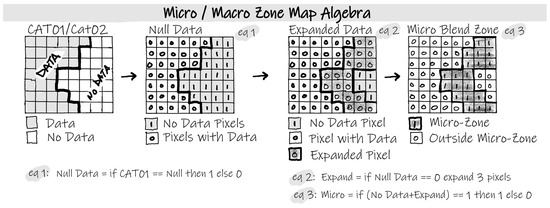
Figure 11.
Illustration of the map algebra expressions used to generate the micro blending zone. The upper left grid represents the CAT01 composite digital elevation model. The upper right grid, labeled Null Data (eq1), is the result of the first expression that identifies no-data pixels as “1” and pixels with data as “0.” An expanded expression is applied to the no data to extend the 0 values out of three pixels, replacing their respective 1 value to create the Expanded Data (eq2) grid at the bottom left. The final expression sums the no-data and Expanded Data grids, then reassigns all the pixels not equal to 1 to 0. This results in the micro blending zone, where 1s indicate the micro zone and 0s are the pixels outside the zone. Each map algebra expression is defined at the bottom with the number corresponding to the equation grid (eq).
2.7. Binary Stacking and Bit-Packing
After creating the 16 binary layers, the next step is to stack these layers and compile them down to 16-bit integer values creating the Bit-pack layer. TEMM primarily uses Python interpretive scripts and the Numpy Python module to convert the geospatial binary layer to a 2D array. The arrays are stacked in the order defined in Figure 7, creating a multidimensional array (Figure 7, Step 1). Each pixel, or element on the z-axis, is read from the top of the axis down, compiling the sequence of 1s and 0s into its respective 16-bit integer, collectively creating the Bit-packed 2D array (Figure 7, Step 2). The Bit-pack array is converted to a readable format like a GeoTIFF with geospatial reference information applied, allowing for further geospatial analysis (Figure 7, Step 3) [WF-10,11].
In the context of TEMM, the Bit-pack and its companion value range table in Appendix B provide a quantitative assessment of each elevation category’s elevation state. How a Bit-pack is interpreted is contingent on its companion documentation and user requirements [WF-2].
2.8. Inverse Weighted Distance Data Interpolation Methods
The inverse distance weighting (IDW) interpolation method is a foundation for blending inside the micro and macro zones. Below are the three composite blending methods that leverage IDW to transition between disparate datasets.
Weighted Slope Interpolation
The weighted slope interpolation (WSI) approach is applied to the MaBZ, the areas bordering high-resolution bathymetric (HR) data, and extending 50 m over the moderate-resolution bathymetric (MR) data to improve continuity between disparate elevation values. This method does not modify the HR data; the zone extends 50 m over the MR data, creating an interpolated elevation transition that matches the HR perimeter elevation and progressively mimics the underlying MR profile until matching the MR elevation.
To create this progressive transition, the first step is to build a progressive weighted delta surface (Δpw). The Δpw is calculated by obtaining the absolute difference between the IDW interpolated surface (i) and the underlying MR (c) and multiplying that difference value by the ratio of the blending zone’s Euclidean distance (eu) from the maximum eu value (Equation (1)). The resulting Δpw is an adjusted delta surface based on the distance of a pixel from the perimeter of the HR data. The closer a pixel is to the HR’s perimeter, the closer the MR delta (i − c) is to zero. The farther from the HR perimeter, the higher percentage of the MR delta is retained until eu equals 1.
Following applying the Δpw equation, a degree slope derivative from the MR data inside the MaBZ is created to increase the weighting of the delta pixels in the areas of high slope in degrees. Although the Δpw provides a means to generate continuity between these disparate datasets, when there is a high degree of slope; the closer that slope feature is to the HR perimeter, the more muted the slope becomes when just the Δpw is applied. A slope weight is applied to the final equation to preserve more of the slope characteristics. To apply this weighting to the final WSI, a 1 is added to the slope percentage (slope/100) and multiplied by the Δpw to generate the Δws coefficient that then adds the MR (c) to create the WSI surface.
The WSI approach was inspired by the Delta Surface Fill Method by Grohman, Kroenung, and Strebeck (2006) because of its simplicity [16]. Adding progressive and slope weighting provides for the alignment of the interpolated data between two disparate data sources. In contrast, the Delta Surface Fill Method fills the gaps in a single data source. Table 2 and Figure 12 illustrate how the WSI algorithm is applied to a small sample dataset.

Table 2.
Sample data illustrating how the weighted slope interpolation (WSI) is calculated. Column abbreviation titles: Euclidean distance (eu), inverse distance weighting (IDW) interpolated elevation (i), moderate-resolution (MR) bathymetry (c), MR bathymetry slope, applied progressive weight interpolation (Δpw + c), and the last column is the weighted slope interpolation (WSI).
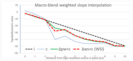
Figure 12.
Sample chart comparing inverse distance weighting (IDW) interpolated profile (black dashed line), source moderate-resolution (MR) profile (blue dotted line), progressive weighted interpolation (Δpw) profile (solid green line), and the slope weighted interpolation (SWI) profile (red dashed line).
Figure 13 illustrates the application of the WSI on a collection of HR and MR datasets at the east entrance to the Canaveral Barge Canal in Florida. HR data are available on both the north and south sides of the canal, but the canal only has MR data available. The top three maps from the left to right represent an unblended mosaic, followed by two blended mosaics. The unblended map represents a composite DEM where all the datasets are merged based on priority. The middle map used IDW interpolation applied in the MaBZ, shown by the semitransparent band adjacent to the HR data and overlapping the MR data. The right map has the WSI blending applied to the MaBZ. The vertical line in each map represents the profile transect graphed in the chart below. The color of the transect in the map correlates to the elevation profile graphic in the chart. The gray boxes in the graph correspond to the MaBZ to highlight this zone (Figure 13).
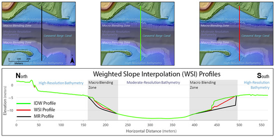
Figure 13.
This series of maps and profile graph shows the change in bathymetric values inside the macro blending zone (MaBZ) from an unblended digital elevation model (DEM), inverse distance weighting (IDW) interpolation, and weighted slope interpolation (WSI). The top left map is an unblended composite DEM, and the middle map is the same composite with an IDW interpolation applied in the zone. The right map is the same composite with the WSI applied in the zone. The elevation profile chart graphs each transect, and the line color corresponds to the respective map on which the transect is located.
Input Minimum Value (INMIN)
When the input minimum value (INMIN) is assigned to a pixel, the minimum elevation value from any valid input in the MiBZ is applied. As indicated in Appendix B, Table A1 in the INMIN row, when there is no valid high-resolution topographic elevation below MSL (CAT01) or no valid topobathymetric (CAT02) data source available in the MiBZ, that pixel is filled with the minimum value of the remaining contributing composite categories, including the IDW interpolated surface (Figure 14). The INMIN is applied to a narrow band of conditions in the MiBZ. The first condition is a data anomaly that occurs when a CAT02 indicates an elevation above MSL and the CAT05 hydro-flattened surface is below MSL; this contrast in values typically happens when topobathymetric lidar has gaps in the collection in the urbanized nearshore areas between the values below MSL and razed surface like dock and piers that result in an erroneous above-MSL interpolation. The other occurrence is in the absence of CAT01 and CAT02 pixels when the CAT05 hydro-flattened surface is below MSL, and the CAT06 indicates a pixel value above MSL.
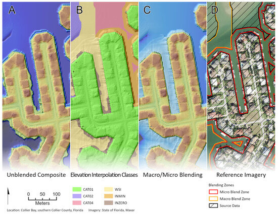
Figure 14.
Panel (A) shows an unblended composite digital elevation model (DEM) as context to show how and where pixels are modified during this step. Panel (B) shows what category composite DEMs or blending methods are applied to create a micro/macro blended DEM. CAT01, CAT02, and CAT04 indicate the use of those respective composite DEMs, WSI indicates the use of the weighted slope interpolations, INMIN indicates the use of the input minimum value method, and INZERO indicates the use of the input zero truncated surface method. Panel (C) shows the results of implementing the interpolation methods indicated in panel B using the micro/macro method. Panel (D) is an aerial image to provide context. The polygons indicate the locations of the micro (red) and macro (orange) zones. The black-hatched polygons are areas where no interpolation is applied.
Input Zero Truncated Surface (INZERO)
The input zero truncated surface (INZERO) only uses the IDW interpolated data source. Based on the Bit-pack assessment, this pixel should be at or below MSL, and no valid inputs meet that requirement. As a result of this assessment, the IDW interpolation is used, and if that IDW elevation is greater than the MSL, it is truncated to zero. This situation typically occurs near the shoreline’s perimeter, where the IDW interpolation may also be above MSL. There is one exception where this is applied outside of a blending zone: when the Bit-pack indicates receded shorelines, and that value range is 2056 through 2300 as depicted in Figure 8 panel C.
2.9. Elevation Classifications of the Bit-Packed Data Layer
The TEMM currently applies three blending methods for transitioning between disparate datasets (Table 3). These methods are based on the IDW interpolation because of its efficient implementation and TEMM’s relatively small voids often surrounded by numerous valid data points [11,17]. In the case of the MaBZ where IDW interpolation accuracy limits diminish, a weighting is applied to it in conjunction with the CAT04, moderate-resolution bathymetric data. To efficiently integrate these methods into a TBDEM, the Bit-pack dataset values are aggregated into eight classes: five of the classes reference the respective elevation categories, and three classes apply an interpolation method. Because an integer’s binary code is a constant, TEMM creates an elevation interpolation classification (EIC) table based on the integer value ranges defined in the value table in Appendix B. An example of a value range is the CAT02 range from 35,840 to 48,380 (binary: 10 00 11 00 00 00 00 00 to 10 11 11 00 11 11 11 00), where the CAT02 elevation takes priority over the CAT01 except when the CAT02 elevation is above MSL where the Bit-pack value is 47,356. Examining the binary code for 47,356 in Figure 15 reveals that the topobathymetric input is sometimes spatially inconsistent because it is not in agreement with the current topographic binary pair (CAT01) input indicating elevation at or below MSL (binary positions 13 and 12) or any of the lower priority categories that also indicate elevations at or below MSL (binary positions 7 through 2) (Figure 15). CoNED’s experience in this situation indicates a high probability that the topobathymetric data have an interpolation error due to gaps in data acquisitions, so in these situations, the topographic elevation (CAT01) takes priority over the topobathymetric (CAT02) elevation.

Table 3.
Elevation interpolation classifications. Classification numbers 1 through 7 apply direct reference to the use of the pixel value from the respective elevation category, except CAT03 and CAT07, which are not used as of publication. Classifications 11, 12, and 13 are modified inverse distance weighting (IDW) interpolation methods.
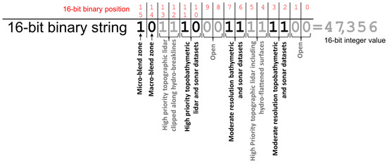
Figure 15.
This binary code for integer 47,356 illustrates how to identify data anomalies by analyzing the sequence of ones and zeros or switches in the binary code. This code sequence reveals that the CAT02 input data are likely errant values because these data deviate from the priority current topographic input, CAT01, as well as from the lower priority inputs.
As with most situations, there are outliers or unique exceptions. For the TEMM, these exceptions are listed at the bottom of the table in Appendix B. The resulting classification lookup table (LUT) lists all the possible integers based on the value ranges and exceptions from this table and assigns the respective EIC to each value. The LUT is joined with the Bit-pack dataset in a one-to-many relationship, and the Bit-pack dataset is aggregated to an EIC raster dataset (Figure 16). This EIC dataset is then used to apply the indicated interpolation to generate the final micro/macro blending zones for inclusion into the final TBDEM [WF-9].
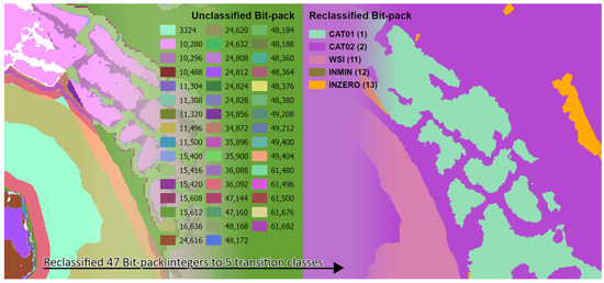
Figure 16.
Example for Bit-pack value range aggregation. On the left is the original Bit-pack result for a spatial extent with unique values. The right is the results of joining the classification lookup table (LUT) with the Bit-pack dataset and aggregating to the elevation interpolation classification (EIC). The EIC has a potential of eight classes, but in this example spatial extent, only five classes are indicated.
2.10. Creating the Micro and Macro Elevation Interpolation
Six high-level processes create the final micro and macro interpolated blending layer [WF-14] (Figure 17). Step 1: Create an interim DEM by merging all the input datasets based on priority as defined in Danielson and others (2016) (Figure 17A) [3]. Step 2: Generate a blending mask from the EIC dataset by removing all the pixels in the blending zones that require interpolation (Figure 17B). Step 3: Extract data from the interim DEM that intersects the blending mask. The resulting masked DEM will have the areas requiring interpolation set to Null or no data (Figure 17C). Step 4: Apply an IDW interpolation to the masked DEM, creating a new DEM with interpolated elevation values over the blending zones (Figure 17D). Step 5: Apply the defined interpolation method to the blending zones. This step has three independent operations listed below that are applied before moving to the final step.
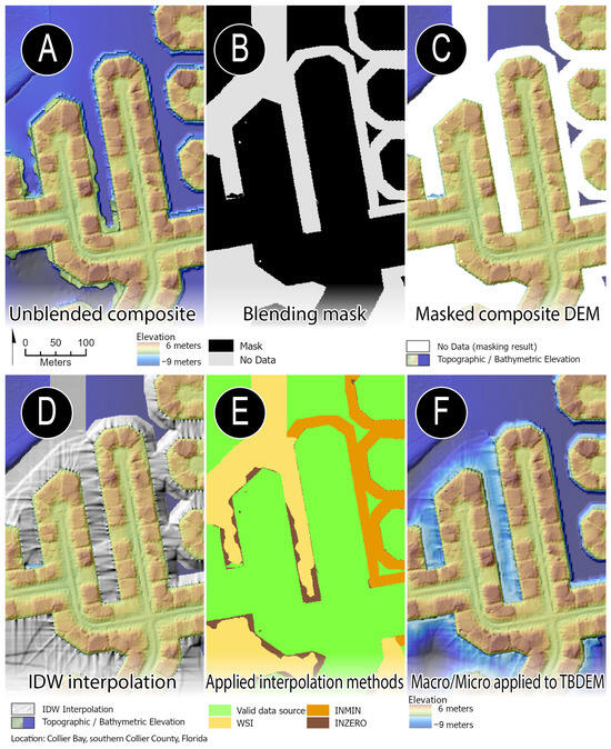
Figure 17.
Visual representation of the six high-level steps of applying the micro/macro interpolation blending and applying it to the final topobathymetric elevation model (TBDEM). Panel (A) shows a composite of the five elevation categories, and panel (B) shows the mask used to remove the blending zones requiring interpolation. Panel (C) shows the results of removing those blending zones. Panel (D) shows the results of the inverse distance weighting (IDW) interpolation of the blending zones. Panel (E) indicates where the three blending methods (input minimum value [INMIN], input zero truncated surface [INZERO], and weighted slope interpolation [WSI]) will be applied; the green shade refers to valid input data. Panel (F) shows applied blending to zones in the final TBDEM product.
- Apply the WSI (Class no. 11) to the MaBZ.
- Select the minimum elevation value from all the input sources, including the IDW interpolated layer from the INMIN class (Class no. 12).
- Apply the IDW interpolated data to the MiBZ with values greater than MSL clipped to MSL for the INZERO class (Class no. 13).
Step 6 merges the results of the individual operations into a single blended dataset (Figure 17F) [WF-17]. This new blended DEM will be set as the top priority in the TEMM priority list as part of step 5 of the integration component of the TEMM [3] [WF-19].
3. Discussion
This new micro/macro blending method improves the quality and efficiency of producing regional-scale TBDEMs. Two key benefits are the automated process of removing receded shoreline artifacts and smoothing the transition between high-resolution bathymetric data and coarser interpolated bathymetric models, but there are limitations. In CoNED TBDEM’s large regional datasets, there are areas with insufficient information to make an informed decision. As more topobathymetric and bathymetric data are collected, these areas will decrease. Currently, the blending uses past elevation data to build the binary stack that defines the blending interpretation method of adjacent data for near-shore and between high- and coarser-resolution bathymetric data. There are opportunities to enhance its blending approach further by introducing additional ancillary data into the stack of binary layers. Examples of the binary layer could be derivatives based on land use/land cover products, spectral imagery to interpret relative bathymetric trends (depths trending deeper or shallower), and other geospatial data to guide its interpolation methods. Alternative interpolation algorithms could be introduced, including artificial intelligence, which can potentially be used to drive interpolations.
The challenge for this application type is quantifying the degree to which the data have been improved. Because this approach addresses improving data in locations where data acquisitions are challenging, like shallow turbid waters and deeper turbid waters in the littoral zone, it is also difficult to validate these data in the bathymetric domain. More control point availability would be necessary to quantify the data model quality in the bathymetric domain [12]. The alternative to using survey-grade validation sites is to assess relative accuracy against the existing high-resolution topobathymetric datasets. A relative accuracy assessment was applied to two representative sites for the MiBZs and MaBZs. The relative root mean square error (RMSE) was calculated against a topobathymetric control dataset for the two representative areas. The control dataset covering the Indian River Lagoon on the east-central coast of Florida lidar was acquired in June 2022. It has a submerged vertical accuracy of ±29.1 cm [18]. When compared against this control, the blending method does show an improvement in data quality for both the micro and macro blending zones compared to the original unblended TEMM. The MiBZ and MaBZ RMSE values are 0.147 and 0.126, respectively, with the unblended RMSE of 0.203 for the MiBZ and 0.241 for the MaBZ (Figure 18 and Figure 19). A typical artifact addressed by this blending approach is the reveal of old shorelines that have receded, as shown in Figure 18. Macro blending addresses the elevation offsets at the intersection of high-resolution bathymetric data and coarser resolution or broadly interpolated models, as shown in Figure 19. It is also important to note that the method can improve values in the zones; these improvements will typically fall in the conservative submerged error range for topobathymetric lidar between 10 and 50 cm.
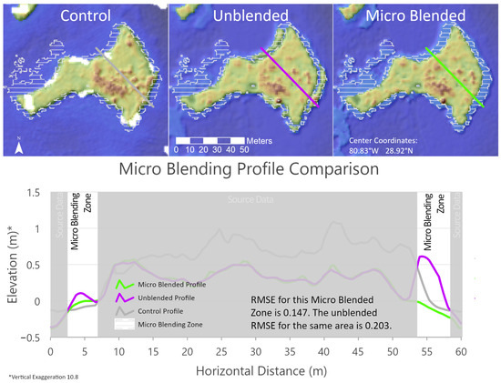
Figure 18.
Illustration of the quantitative micro blending zone root mean squared error (RMSE) analysis results. The three-color shaded relief maps represent the data sources used in the RMSE analysis. The top left map represents the topobathymetric control data source, the middle map represents the unblended topobathymetric elevation modeling method (TEMM) topobathymetric elevation model (TBDEM), and the map on the right represents the micro blending method. The white horizontal hatch feature in all the maps represents the area where the micro blending occurred and is the area used to derive the RMSE values. The line segments on the maps represent the elevation profile chart below the maps. The line color in each map corresponds to the profile on the chart. The white segments on the chart are the intersection of the elevation profiles and the micro blending zone analysis. The gray areas on the chart are the segments along the profile that reflect the source elevations with no interpolation. Note that the elevation range on the y-axis is 1.5 m, well within the error range of the typical submerged topobathymetric measurements. The white patches in the control map are areas where no valid lidar point could be acquired.
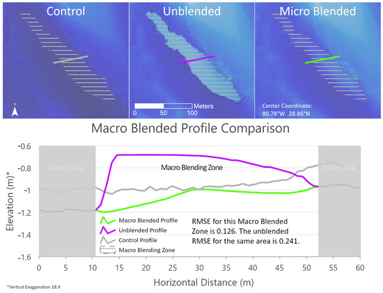
Figure 19.
Illustration of the quantitative macro blending zone root mean squared error (RMSE) analysis results. The three-color shaded relief maps represent the data sources used in the RMSE analysis. The top left map represents the topobathymetric control data source, the middle map represents the unblended topobathymetric elevation modeling method (TEMM) topobathymetric elevation model (TBDEM), and the map on the right represents the macro blending method. The white horizontal hatch feature in all the maps represents the area where the macro blending occurred and is the area used to derive the RMSE values. The line segments on the maps represent the elevation profile chart below the maps. The line color in each map corresponds to the profile on the chart. The white segment on the chart is the intersection of the elevation profiles and the macro blending zone analysis. The gray areas on the chart are the segments along the profile that reflect the source elevations with no interpolation. Note that the elevation range on the y-axis is 2 m, well within the error range of the typical submerged topobathymetric measurements.
4. Conclusions
The Coastal National Elevation Database (CoNED) Applications Project’s topobathymetric elevation modeling method (TEMM) provides a unique approach for integrating disparate data sources to create regional seamless topobathymetric coastal digital elevation models (TBDEMs). However, the increased complexity of the data integration process due to the improved accuracy and frequency of topobathymetric acquisitions has resulted in increased disparities in adjacent datasets. To mitigate these vertical differences between neighboring datasets, the CoNED Applications Project has leveraged the fundamental principle of binary notation to develop a quantitative data layer that collectively assesses input elevation models at the pixel level. This pixel-level assessment data layer, the Bit-pack, allows the project to efficiently identify and mitigate previously manually corrected or undetected artifacts. The principles of this Bit-packing approach satisfy the project’s current requirements of providing continuous regional TBDEMs that are composited with the best available data. The test sample RMSE values for the micro (MiBZ) and macro (MaBZ) blending zones are 0.147 and 0.126, respectively, while the unblended RMSE values are 0.203 for the MiBZ and 0.241 for the MaBZ. The blending method improves data quality for both the micro and macro blending zones compared to the original unblended TEMM. As higher-quality data becomes available, this dynamic approach allows the opportunity to introduce additional variables to adapt the method to meet future requirements. Using the resulting Bit-pack data layer to implement multiple blending interpolation methods between disparate inputs is a predictable method to produce consistent outcomes that can improve transitions between disparate bathymetric data and enhance the TBDEM product.
Author Contributions
Conceptualization, D.J.T.; Methodology, W.M.C.; Writing—original draft, W.M.C. All authors have read and agreed to the published version of the manuscript.
Funding
This research was funded by the U.S. Geological Survey Coastal and Marine Hazards and Resources Program (CMHRP).
Data Availability Statement
The original contributions presented in the study are included in the article, further inquiries can be directed to the corresponding author.
Acknowledgments
Any use of trade, firm, or product names is for descriptive purposes only and does not imply endorsement by the U.S. Government.
Conflicts of Interest
The authors declare no conflict of interest.
Appendix A. Micro-Macro Blending Method Flow Diagram
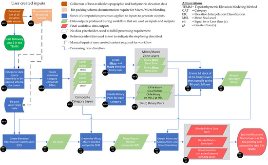
Figure A1.
This is a general high-level workflow (WF) diagram of the topobathymetric elevation modeling method (TEMM) integration component (TIC) micro/macro blending method. Each step (process or output) is notated with a WF and number (WF-N) inside a black circle. These step notations are referenced in the text to visually illustrate where in the workflow each process and output occurs.
Appendix B. Micro and Macro Blending Zone Binary Value Range Table
The value range table is used to build a lookup table (LUT) defining the elevation interpolation classes for every 16-bit unsigned integer (0–65,534) (Table A1). Based on the value ranges described in this table, 772 integers have an assigned interpolation class, and the remaining values are ignored. The value range table is a representative snapshot and is not intended to be a constant. Depending on the input sources, it may need modification, and because it can be altered, including a version of the table is warranted as a part of the metadata package. Individual value exceptions may fall inside a range, which are listed in the table following the defined value ranges. The topobathymetric elevation modeling method (TEMM) algorithm replaces the initial class assignment with the exception class following the initial build of the LUT. There are two conditions when a value is ignored. (1) When any binary pair’s first value is 0 and the second is 1. This combination is not logical for the micro/macro blending method. There cannot be a pixel indicating no data, represented by a 0 in the first position, and that the same pixel’s value is at or below mean sea level (MSL), represented by a 1 in the second position (“01”). (2) At publication, four positions in the binary code are not being used: positions 9 and 8, and 1 and 0 moving left to right. Any binary code where these positions are set to 1 is ignored.

Table A1.
Bit-pack value range lookup table.
Table A1.
Bit-pack value range lookup table.
| Elevation Interpolation Value Range Rules | ||||||
|---|---|---|---|---|---|---|
| Class Number | Class Abbreviation | Interpolation Description | Value Range | Binary Code Range | ||
| Minimum | Maximum | Minimum | Maximum | |||
| 1 | CAT01 | Use CAT01 elevation category values. | 8192 | 10,492 | 00 10 00 00 00 00 00 00 | 00 10 10 00 11 11 11 00 |
| 12,288 | 12,540 | 00 11 00 00 00 00 00 00 | 00 11 00 00 11 11 11 00 | |||
| 24,608 | 24,828 | 00 10 10 00 11 11 11 00 | 00 11 10 00 00 00 10 00 | |||
| 57,344 | 63,740 | 11 10 00 00 00 00 00 00 | 11 11 10 00 11 11 11 00 | |||
| 2 | CAT02 | Use elevation category values. | 2048 | 2284 | 00 00 10 00 00 00 00 00 | 00 00 10 00 11 10 11 00 |
| 3080 | 3324 | 00 00 11 00 00 00 10 00 | 00 00 11 00 11 11 11 00 | |||
| Use CAT02 when both CAT01 and CAT02 have valid data falling at or below mean sea level (MSL) in the micro zone and have an overlap of the micro and macro zones. | 11,264 | 11,516 | 00 10 11 00 00 00 00 00 | 00 10 11 00 11 11 11 00 | ||
| 15,360 | 15,612 | 00 11 11 00 00 00 00 00 | 00 11 11 00 11 11 11 00 | |||
| 35,840 | 48,380 | 10 00 11 00 00 00 00 00 | 10 11 11 00 11 11 11 00 | |||
| 64,512 | 64,764 | 11 11 11 00 00 00 00 00 | 11 11 11 00 11 11 11 00 | |||
| 4 | CAT04 | Use CAT04 elevation category values. | 128 | 252 | 00 00 00 00 10 00 00 00 | 00 00 00 00 11 11 11 00 |
| 5 | CAT05 | Use CAT05 elevation category values. | 32 | 60 | 00 00 00 00 00 10 00 00 | 00 00 00 00 00 11 11 00 |
| 6 | CAT06 | Use CAT06 elevation category values. | 8 | 12 | 00 00 00 00 00 00 10 00 | 00 00 00 00 00 00 11 00 |
| 11 | WSI | Weighted slope interpolation for all the pixels located in the macro blending zone. | 16,392 | 16,636 | 01 00 00 00 00 00 10 00 | 01 00 00 00 11 11 11 00 |
| 49,160 | 49,404 | 11 00 00 00 00 00 10 00 | 11 00 00 00 11 11 11 00 | |||
| 12 | INMIN | Minimum input pixel value from overlapping elevation inputs. | 44 | 60 | 00 00 00 00 00 10 11 00 | 00 00 00 00 00 11 11 00 |
| 32,776 | 32,952 | 10 00 00 00 00 00 10 00 | 10 00 00 00 10 11 10 00 | |||
| 51,212 | 51,452 | 11 00 10 00 00 00 11 00 | 11 00 10 00 11 11 11 00 | |||
| 13 | INZERO | Inverse distance weighting (IDW) interpolation truncated to zero or below (maximum value is zero). | 2296 | 2300 | 00 00 10 00 11 11 10 00 | 00 00 10 00 11 11 11 00 |
| 14,344 | 14,588 | 00 11 10 00 00 00 10 00 | 00 11 10 00 11 11 11 00 | |||
| 28,680 | 28,924 | 01 11 00 00 00 00 10 00 | 01 11 00 00 11 11 11 00 | |||
| 33,008 | 35,068 | 10 00 00 00 11 11 00 00 | 10 00 10 00 11 11 11 00 | |||
| Elevation interpolation value range exceptions | ||||||
| 1 | CAT01 | 47,144 | 10 11 10 00 00 10 10 00 | |||
| 47,160 | 10 11 10 00 00 11 10 00 | |||||
| 2 | CAT02 | 34,848 | 10 00 10 00 00 10 00 00 | |||
| 34,976 | 10 00 10 00 10 10 00 00 | |||||
| 34,984 | 10 00 10 00 10 10 10 00 | |||||
| 5 | CAT05 | 16,416 | 01 00 00 00 00 10 00 00 | |||
| 32,800 | 10 00 00 00 00 10 00 00 | |||||
| 32,808 | 10 00 00 00 00 10 10 00 | |||||
| 49,184 | 11 00 00 00 00 10 00 00 | |||||
| 13 | INZERO | 2056 | 00 00 10 00 00 00 10 00 | |||
| 2060 | 00 00 10 00 00 00 11 00 | |||||
| 2088 | 00 00 10 00 00 10 10 00 | |||||
| 2248 | 00 00 10 00 11 00 10 00 | |||||
| 2252 | 00 00 10 00 11 00 11 00 | |||||
| 32,768 | 10 00 00 00 00 00 00 00 | |||||
| 32,992 | 10 00 00 00 11 10 00 00 | |||||
| 35,068 | 10 00 10 00 11 11 11 00 | |||||
| 47,164 | 10 11 10 00 00 11 11 00 | |||||
| 47,352 | 10 11 10 00 11 11 10 00 | |||||
| 47,356 | 10 11 10 00 11 11 11 00 | |||||
| 49,152 | 11 00 00 00 00 00 00 00 | |||||
| 61,496 | 11 11 00 00 00 11 10 00 | |||||
| Elevation interpolation exclusion value range | ||||||
| NA | Exclude | Any binary pair where the first value is 0 and the second is 1. This combination is not logical, because there cannot be a pixel with no data and indicate that value is at or below MSL. | All these possible values where a “1” is present in these positions are calculated by the algorithm. Example binary code 00 01 01 01 01 01 01 01 | |||
| NA | Exclude | When open CAT03 has a one in either position (9 or 8) or when open CAT07 has a one in either position (1 or 0). | All these possible values where a “1” is present in these positions are calculated by the algorithm. Example binary code 00 10 10 11 10 10 10 11 | |||
References
- Pricope, N.G.; Bashit, M.S. Emerging trends in topobathymetric LiDAR technology and mapping. Int. J. Remote Sens. 2023, 44, 7706–7731. [Google Scholar] [CrossRef]
- Gesch, D.; Wilson, R. Development of a seamless multisource topographic/bathymetric elevation model of Tampa Bay. Mar. Technol. Soc. J. 2001, 35, 58–64. [Google Scholar] [CrossRef][Green Version]
- Danielson, J.J.; Poppenga, S.K.; Brock, J.C.; Evans, G.A.; Tyler, D.J.; Gesch, D.B.; Thatcher, C.A.; Barras, J.A. Topobathymetric elevation model development using a new methodology—Coastal National Elevation Database. J. Coast. Res. 2016, 76, 75–89. [Google Scholar] [CrossRef]
- Interagency Working Group on Ocean and Coastal Mapping. Standard Ocean Mapping Protocol; National Oceanic and Atmospheric Administration (NOAA): Washington, DC, USA, 2024; p. 157. Available online: https://iocm.noaa.gov/standards/SOMPFinal2024.pdf (accessed on 11 September 2024).
- Petrasova, A.; Mitasova, H.; Petras, V.; Jeziorska, J. Fusion of high-resolution DEMs for water flow modeling. Open Geospat. Data Softw. Stand. 2017, 2, 6. [Google Scholar] [CrossRef]
- Fuss, C.E.; Berg, A.A.; Lindsay, J.B. DEM Fusion using a modified k-means clustering algorithm. Int. J. Digit. Earth 2016, 9, 1242–1255. [Google Scholar] [CrossRef]
- Yue, L.; Shen, H.; Zhang, L.; Zheng, X.; Zhang, F.; Yuan, Q. High-quality seamless DEM generation blending SRTM-1, ASTER GDEM v2 and ICESat/GLAS observations. ISPRS J. Photogramm. Remote Sens. 2017, 123, 20–34. [Google Scholar] [CrossRef]
- Alemam, M.K.; Yong, B.; Sani-Mohammed, A. A proposed merging methods of digital elevation model based on artificial neural network and interpolation techniques for improved accuracy. Artif. Satell. 2023, 58, 122–170. [Google Scholar] [CrossRef]
- Dong, G.; Huang, W.; Smith WA, P.; Ren, R. Filling voids in elevation models using a shadow-constrained convolutional neural network. IEEE Geosci. Remote Sens. Lett. 2020, 17, 592–596. [Google Scholar] [CrossRef]
- Khojasteh, D.; Chen, S.; Felder, S.; Heimhuber, V.; Glamore, W. Estuarine tidal range dynamics under rising sea levels. PLoS ONE 2021, 16, e0257538. [Google Scholar] [CrossRef] [PubMed]
- Eakins, B.W.; Grothe, P.R. Challenges in building coastal digital elevation models. J. Coast. Res. 2014, 30, 942–953. [Google Scholar] [CrossRef]
- Amante, C.J.; Love, M.; Carignan, K.; Sutherland, M.G.; Macferrin, M.; Lim, E. Continuously updated digital elevation models (CUDEMs) to support coastal inundation modeling. Remote Sens. 2023, 15, 1702. [Google Scholar] [CrossRef]
- Leibniz, G. Explication de l’Arithmétique Binaire. In Die Mathematische Schriften; Mathematical Writings VII; Gerhardt: Königswinter, Germany, 1703; p. 223. [Google Scholar]
- Renslow, M.S. Manual of Airborne Topographic Lidar; American Society for Photogrammetry Remote Sensing: Baton Rouge, LA, USA, 2012. [Google Scholar]
- Heidemann, H.K. Lidar Base Specification; Techniques and Methods; U.S. Geological Survey: Reston, VA, USA, 2018; p. 101. [CrossRef]
- Grohman, G.; Kroenung, G.; Strebeck, J. Filling SRTM voids: The delta surface fill method. Photogramm. Eng. Remote Sens. 2006, 72, 213–216. [Google Scholar]
- Clarke, K.C. Analytical and Computer Cartography, 2nd ed.; Prentice Hall: Englewood Cliffs, NJ, USA, 1995; p. 251. [Google Scholar]
- Dewberry Engineers Inc. Indian River Lagoon Topobathy Shoreline; National Oceanic and Atmospheric Administration: Tampa, FL, USA, 2023.
Disclaimer/Publisher’s Note: The statements, opinions and data contained in all publications are solely those of the individual author(s) and contributor(s) and not of MDPI and/or the editor(s). MDPI and/or the editor(s) disclaim responsibility for any injury to people or property resulting from any ideas, methods, instructions or products referred to in the content. |
© 2024 by the authors. Licensee MDPI, Basel, Switzerland. This article is an open access article distributed under the terms and conditions of the Creative Commons Attribution (CC BY) license (https://creativecommons.org/licenses/by/4.0/).