Abstract
Urbanization is growing at a rapid pace, and this is being reflected in the rising energy consumption from fossil fuels, which is contributing significantly to greenhouse gas impacts and carbon emissions (CE). Aiming at the problems of the time delay, inconsistency, uneven spatial coverage scale, and low precision of the current regional carbon emissions from energy consumption accounting statistics, this study builds a precise model for estimating the carbon emissions from regional energy consumption and analyzes the spatio-temporal characteristics. Firstly, in order to estimate the carbon emissions resulting from energy consumption, a fixed effects model was built using data on province energy consumption and NPP-VIIRS-like nighttime lighting data. Secondly, the PRD urban agglomeration was selected as the case study area to estimate the carbon emissions from 2012 to 2020 and predict the carbon emissions from 2021 to 2023. Then, their multi-scale spatial and temporal distribution characteristics were analyzed through trends and hotspots. Lastly, the influence factors of CE from 2012 to 2020 were examined with the OLS, GWR, GTWR, and MGWR models, as well as a ridge regression to enhance the MGWR model. The findings indicate that, from 2012 to 2020, the carbon emissions in the PRD urban agglomeration were characterized by the non-equilibrium feature of “high in the middle and low at both ends”; from 2021 to 2023, the central and eastern regions saw the majority of its high carbon emission areas, the east saw the region with the highest rate of growth, the east and the periphery of the high value area were home to the area of medium values, while the southern, central, and northern regions were home to the low value areas; carbon emissions were positively impacted by population, economics, land area, and energy, and they were negatively impacted by science, technology, and environmental factors. This study could provide technical support for the long-term time-series monitoring and remote sensing inversion of the carbon emissions from energy consumption in large-scale, complex urban agglomerations.
1. Introduction
China, as a “coal-rich, oil- and gas-poor” country, has become the world’s largest energy consumer, top oil importer, and second-largest LNG importer. In 2017, China’s fossil fuel carbon dioxide emissions reached 36.3 billion tons, over one-third of the global total, according to the International Energy Agency (IEA) [1]. As of the present, China is one of the biggest global producer of carbon dioxide, with emissions from fossil fuel usage reaching 6027 million tons: 5769 million tons higher than that of the US. China pledged to reduce carbon emissions by reaching carbon neutrality by 2060 and peak carbon by 2030, and it inaugurated its carbon emissions trading system (ETS) in 2017 [2]. China’s carbon emissions appear to have stabilized in 2017–2019 after declining steadily between 2013 and 2016. China will continue to need more energy overall. There will be more pressure to attain the carbon neutrality targets and complete the energy transformation [3]. In order to promote low-carbon growth while reducing carbon emissions, it is imperative to solve the pressing issues related to energy utilization efficiency, energy transition, total energy demand control, and carbon emission regulation strengthening. Regional initiatives are needed to solve this issue, particularly with regard to reducing the carbon emissions from cities.
Cities are hubs of human activity and have a big impact on the surface of the planet. In addition to concentrating intensive energy consumption and causing significant changes in land use, rapid urbanization also contributes significantly to atmospheric carbon dioxide emissions. According to some research, around 75% of carbon emissions worldwide are produced in urban areas [4]. Moreover, UN-Habitat projected that by 2030, the proportion of carbon emissions from urban areas would rise to 76% [5]. Therefore, cutting carbon emissions in cities is crucial to the process of cutting carbon emissions worldwide [6]. The Pearl River Delta (PRD) urban agglomeration in China is highly developed, with the highest carbon emissions and energy consumption, primarily from coal, oil, natural gas, and electricity. Fast growth in construction, transportation, and industry keeps carbon emissions high in this area. In 2019, the Guangdong province accounted for about 10% of the nation’s energy consumption and 12% of its carbon emissions. The PRD is promoting energy restructuring, clean energy development, and green, low-carbon growth. Investigating its energy consumption and carbon emissions is vital for low-carbon development and environmental sustainability.
Conventional research has assessed the carbon emissions associated with residential energy usage at the federal level and examined the factors influencing them. Liu et al., for instance, looked at how rising household consumption affected carbon emissions in China’s cities [7]. Although the power demand is rising, coal consumption is rapidly declining. Carbon emission variations are influenced by urbanization and population growth. Zhao et al. observed a shift towards an energy-intensive household consumption structure and cleaner, higher-quality energy sources like natural gas, oil, and electricity, aiming for greater comfort and environmental friendliness [8]. Zheng et al.’s analysis of China’s 2012 home energy usage is based on specific information from 1450 families that were polled [9]. Chen and colleagues developed regression models considering temperature and socio-economic factors to measure global residential fuel and electricity usage and to simulate monthly household energy consumption and emissions, which indicated that population growth and economic success significantly influence energy consumption changes [10]. Li et al. used the input–output method to assess Chinese households’ direct and indirect CO2 emissions from 1996 to 2012. They found that urban homes produced more CO2 than rural homes, with indirect emissions being significantly higher than direct ones. Urban direct emissions were slightly higher than rural, and emissions from different fuels varied between urban and rural households [11]. The methodology employed by Zhu et al. relied upon the spatial mapping relationship between entity locations and multi-source data, as the Intergovernmental Panel on Climate Change (IPCC) also recommends adopting the coefficient method to calculate emissions. The results show that in contrast to other places, industrial and transportation zones have much greater pollutant emission intensities [12].
Although statistical data has been used in the majority of prior studies to compute the carbon emissions from energy usage, there are still certain limitations. For instance, there may be significant discrepancies in the macro statistics between local and national data sources in China [13], the township-level usage of energy data are hardly ever accessible, and administrative boundaries significantly restrict regional figures [14]; furthermore, a variety of respondent samples have a significant impact on the outcomes of microsurveys, and creating the questionnaires takes a lot of time and work [15]. As a result, it is challenging to produce a nationally representative geographic reproduction of emissions [16], and it is necessary to find different pathways to model carbon emissions from energy consumption.
Currently, the illumination observed at night can serve as a useful indicator of economic activity [17], and it has been applied frequently in research to calculate the carbon emissions from energy consumption. Su et al. (2014), for example, using DMSP/OLS evening light images, developed a standardized method to evaluate the usage of energy and carbon dioxide emissions at the city level in China. The main drivers for proposing feasible mitigation solutions were examined [18]. Using DMSP/OLS nighttime lighting data and provincial energy statistics yearbook data, Wang et al. constructed an accurate estimation model for CO2 emissions in Chinese cities, and calculated and analyzed the growth of built-up urban area and carbon emissions in different time periods for the whole country and for the four major economic zones in China [19]. Fang et al. estimated the carbon emissions of 282 Chinese cities from 2004 to 2018 based on nighttime lighting data and measured the carbon emission efficiency (CEE) [20]. The carbon emission statistics and nighttime steady light (NSL) data from the Nighttime Linear Scanning System of the Defense Meteorological Satellite Program (DMSP-OLS) were combined and a standardized technique for estimating the usage of energy and China’s urban emissions of carbon dioxide was established by Shi et al. (2016). In order to mimic the spatiotemporal dynamics of CO2 emissions in China at a greater resolution, they also suggested a panel data analysis approach. The findings demonstrated a positive link between the provincial-level NSL data and China’s statistics for the CO2 emissions from 1997 to 2012. This method can be utilized for the estimation of CO2 emissions at a 1 km resolution [21]. Zheng et al. used the OLS model to analyze data from the DMSP and nighttime light data from the VIIRS, integrated into NPP composite data, to estimate the energy carbon emissions from 2000 to 2019 and to analyze the carbon footprint and carbon deficit dynamics at different scales in the Yellow River Basin [22].
Furthermore, developing low-carbon policies and comprehending the dynamics of the carbon cycle depend on the precise modeling of urban CO2 emissions. An enhanced night-lighting-based method was created by Han et al. to simulate urban CO2 emissions and look into their temporal and spatial patterns. Unlike earlier approaches, the study upgraded the current CO2 inventory from the national and provincial levels to the city level and fixed the saturation issue of nighttime lights to further examine evening light performance on a more detailed basis [23]. In part, the statistical data gap was supplied by the revised data on nighttime light. Yang et al. proposed a neural network model (NNEnsemble) to address inaccuracies in city-scale carbon emission statistics that did not reflect the nonlinear link between provincial emissions and nighttime steady light (NSL) data from the DMSP-OLS satellite. They used a weighting coefficient technique with NSL data to estimate urban carbon emissions, and the method outperformed comparable approaches across all the evaluation indices [24]. To accomplish the spatial refinement of carbon emission and energy consumption measurements, Wang et al. built a carbon energy-estimating model using multi-source remote sensing data and examined the factors that affect carbon emissions and energy usage [25]. Some entities find it difficult to build inventory procedures for local communities because of a lack of data. A top-down method for estimating CO2 emissions utilizing statistical energy data and nighttime light photography was presented by Meng et al., and they found that evening light imaging is appropriate for city-scale CO2 calculations [26].
Both the methodology for variable testing and the foundation for data selection were considered in the current investigation. On the one hand, compared to the original DMSP-OLS data, the NPP-VIIRS data are more accurate at predicting socio-economic data distributions, thanks to the release of the first global Suomi National Polar Orbiting Partnership (NPP) Visible Infrared Imaging Radiometer Suite (VIIRS) nighttime light composite data [27]. Some researchers have also compared the performance of the two forms of nighttime illumination data. For instance, Zhao et al. examined the performance of the NPP-VIIRS data by contrasting it with the raw and saturation-corrected DMSP-OLS data. Lastly, detailed investigations into the geographical characteristics were conducted at the prefectural, province, and regional levels. The results show that the NPP-VIIRS data perform better in statistical regression and spatial comparison [28]. In terms of its on-board calibration, radiometric detection range, and spatial and radiometric resolution, NPP-VIIRS performs better than DMSP-OLS [29]. In particular, NPP-VIIRS has a very strong association with population economic metrics, the GDP, electric power consumption, and other socio-economic characteristics, making it potentially useful for mapping socio-economic activities [30,31,32]. However, there are few studies modeling Chinese carbon emissions using the NPP-VIIRS data and even fewer examining the first-order difference series’ smoothness or the long-term association between carbon emissions and nighttime lighting values (DN). Most research relies on panel data to establish carbon emission models and conduct spatio-temporal analyses.
Therefore, the above studies mainly have the following problems: (1) The statistical data have problems such as incompleteness, inconsistency, and time lag, which make it difficult to truly reflect the spatial carbon emissions. (2) Because nighttime illumination data can represent the spatial distribution of human activities, they are frequently used to estimate variables such as economic activity, population distribution, and energy consumption (e.g., DMSP/OLS and VIIRS data). However, a single nighttime lighting datum also suffers from outliers, oversaturation, and other problems in its application. (3) Although panel unit root tests and panel data cointegration tests have important applications in economics and econometrics, there are fewer related studies. This study estimated the energy consumption carbon emissions from 2012 to 2020 and forecasted the emissions for 2021 to 2023 using NPP-VIIRS-like nighttime lighting data in the PRD. It conducted panel unit root and cointegration tests with provincial energy carbon emission data, selecting the fixed effect model based on precision evaluation. This study examined the spatial and temporal distribution of carbon emissions and used an MGWR model extended by ridge regression to analyze the factors affecting the PRD’s carbon emissions and energy consumption.
This study primarily contributes to the following three areas:
- (1)
- In order to fill in the gaps in this field, this study uses the panel unit root test to confirm the smoothness of the first-order difference series of variables related to carbon emissions and the panel data cointegration test to look into the long-term relationship between carbon emissions and nighttime lighting values (DN).
- (2)
- To verify the fixed effects model’s reliability, this study contrasts it with the random effects model (RE) and the mixed estimation model (POOL). As a result, the model with fixed effects was chosen for the estimation and forecast of the carbon emissions from energy consumption in the PRD, since it has the maximum accuracy in estimating carbon emissions.
- (3)
- In light of the MGWR model’s superiority over the OLS, GWR, and GTWR models, as well as its advantages in modeling spatial heterogeneity and performing multi-scale analyses, its flexibility, and the superior interpretability of its results, we selected it to perform a ridge regression to address the multiple covariance problem and analyze the variables impacting the carbon emissions in the PRD; as a result, this work expands upon the MGWR model.
2. Study Areas and Data Sources
2.1. Study Areas
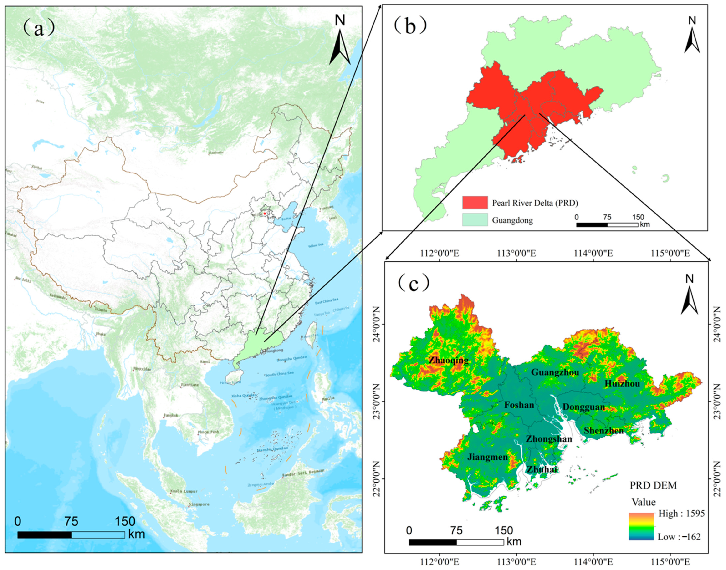
The Pearl River Delta (PRD) region, situated in the south of Guangdong Province, China, is a key economic center and manufacturing base. It benefits from a favorable geographical location, suitable climate, and convenient transportation. The PRD is a low-lying area formed by the confluence of the Xijiang, Beijiang, Dongjiang, and Pearl River, characterized by warm, humid summers and hot, humid winters due to its subtropical monsoon climate. These conditions support agriculture and industry, attracting many people from other regions. Guangzhou, Shenzhen, Zhuhai, Foshan, Dongguan, Zhongshan, Jiangmen, Huizhou, and Zhaoqing are some of the major cities (Figure 1). The PRD is bordered by the South China Sea to the east, Guangxi to the west, and the Yangtze River Delta to the north. Covering approximately 7500 square kilometers, it extends from Guangzhou to the Macau Special Administrative Region in the south. The region is crisscrossed by waterways and canals, with rice paddies that are planted three times a year due to year-round cultivation. One of the most populous areas of China is the PRD, which has seen tremendous expansion in both modern industry and agriculture since the 1980s. The PRD saw tremendous economic growth after China opened up and began to reform in 1978. Its average annual GDP growth rate was 13.45%, which was significantly greater than the national average. Understanding and evaluating the regional distribution of carbon emissions in the PRD and their variations over time is essential, as the region is highly energy-demanding and economically developed.
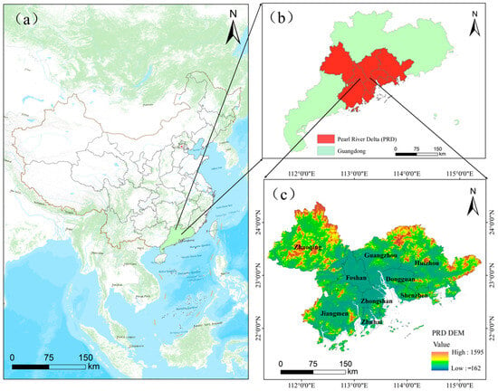
Figure 1.
Overview of the Pearl River Delta region: (a) provincial administrative division map of China; (b) administrative division map of Guangdong Province and the Pearl River Delta; and (c) topographic map of the Pearl River Delta.
2.2. Data Sources
- (1)
- Statistical data
The energy consumption data of the 30 Chinese provinces from 2012 to 2020 (Hong Kong, Taiwan, Macao, and Tibet were excluded from subsequent calculations and analyses due to the lack of data on energy consumption in these regions) in this study were obtained from the China Carbon Accounting Databases (CEADs) and the China Energy Statistical Yearbook of previous years. Then, they were derived from the Provincial Carbon Emission Inventory (PCEI) of the CEAD (China Carbon Accounting Database) for nine different energy sources: raw coal, coke, crude oil, gasoline, kerosene, diesel fuel, fuel oil, liquefied petroleum gas (LPG), natural gas, and electricity. Standard coal’s conversion factor comes from the General Principles for Calculating Comprehensive. The general principles for calculating energy consumption (GB/T 2589-2020) [33] provided the standard coal conversion factor, the 2006 IPCC Guidelines for National Greenhouse Gas Inventories provided the carbon emission factor, and the Guangdong Province’s Statistical Yearbooks from previous years provided the data on the population, economy, science and technology, environment, energy, and land area of the PRD city clusters.
- (2)
- NPP-VIIRS-like nighttime light imagery data
The extended time series of global-level NPP-VIIRS nighttime lighting data (2000–2020) produced by Chen et al. was the source of the 2012–2020 NPP-VIIRS-like nighttime lighting data used in this work. This dataset effectively improves the shortcomings of both DMSP-OLS and NPP-VIIRS nighttime light sources, such as outliers, saturation and non-comparability, effectively extends the time series of the nighttime light images, and is able to clearly reflect the information within the city and its time series changes [34]. The DEM and 2021–2023 NPP-VIIRS data in the PRD were provided by the Resource Environment and Data Center of the Chinese Academy of Sciences. In order to unify the spatial resolution of the multi-source remote sensing data, the 500 m spatial resolution of the nighttime light data was resampled to a 1 km resolution.
- (3)
- Vector data
The 1:1 million data set of the National Geomatics Center of China (NGCC) provided the administrative map of the PRD utilized in this investigation (https://www.webmap.cn, accessed on 15 October 2023), and the online maps in the study area were obtained from the ArcGIS geographic information platform (https://map.wemapgis.com, accessed on 16 October 2023).
3. Methodology
3.1. Research Framework
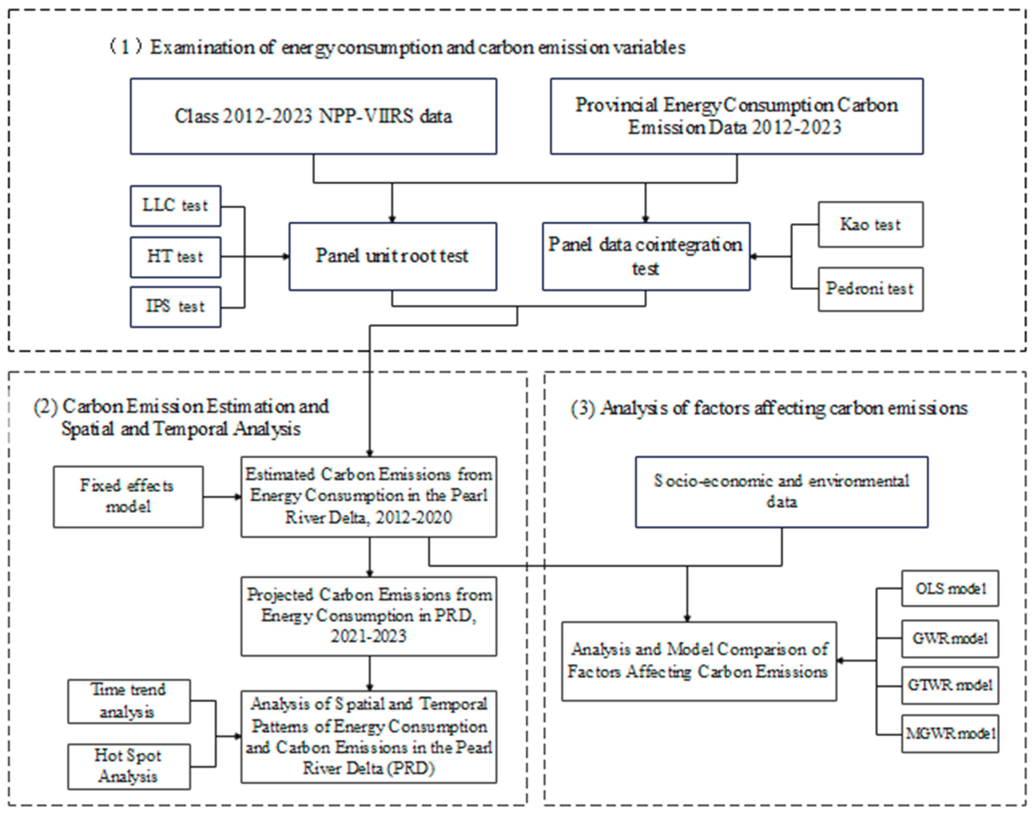
The framework for the study examined the variables that affect carbon emissions, examined the patterns of emissions over time and space, and tested and estimated carbon emission variables based on energy consumption in the PRD. As shown in Figure 2, utilizing preprocessed NPP-VIIRS-like nighttime lighting data and provincial energy and carbon consumption statistics, the study first performed a panel unit root test and a panel data cointegration test. The carbon emissions from 2012 to 2020 were then estimated and the emissions for 2021 to 2023 were anticipated using a fixed effects model. Time trend and hotspot analyses were used to evaluate temporal trends. Lastly, hotspot analyses and precision evaluation techniques were used to look at the patterns of carbon emissions over time and space. The best MGWR model was selected for further study, with a ridge regression of the 2012–2020 PRD carbon emissions as the dependent variable and the demographic, economic, environmental, energy, and land area data as the independent variables.
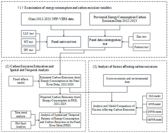
Figure 2.
Study framework diagram.
3.2. Estimation of Carbon Emissions from Energy Consumption Based on Panel Modeling
Common panel data models come in three broad forms: the model of mixed effects, the model of fixed effects, and the model of random effects. The best model was used to estimate the energy consumption carbon emissions of the Pearl River Delta (PRD) urban agglomerations after a comparison and analysis of the best estimation models for building provincial energy consumption carbon emissions.
3.2.1. Model of Mixed Effects (POOL)
A statistical model called a Mixed Effects Model (MEM) was used to examine the data that had a multilevel or grouping structure [35]. When data points are naturally grouped together, this model works especially well. The following equation was fitted using the Mixed Effects Model to the relationship between carbon emissions and evening lighting:
where denotes the carbon emissions resulting from energy consumption in each province, denotes the entire cost of each province’s evening illumination, is the independent variable’s coefficient, denotes the random effect, and denotes the random error term that adheres to the distribution norm with the mean value of 0. i denotes the province, and t denotes the year.
3.2.2. Model of Fixed Effects (FE)
The model of fixed effects (FE) is a statistical model used to deal with the existence of potential unobserved heterogeneity in data and is particularly suitable for dealing with panel data or longitudinal data [36]. Equation (2) illustrates the model setup for the fixed effects model, which was used to fit the link between carbon emissions and evening lights:
where denotes the carbon emissions resulting from energy consumption in each province, denotes total nighttime lighting value in each province, is the predicted coefficient that varies with the individual but does not change over time, and denote the time fixed effect and the individual fixed effect, respectively, and denotes the random error term, obeying the normal distribution with the mean value of . i denotes the province and t denotes the year.
3.2.3. Model of Random Effects (RE)
To investigate how different factors impact observations, a statistical model known as the random effects model (RE) was employed. Because it treats individual differences as random, the random effects model predicts the effects of components more accurately than the fixed effects model [37]. Equation (3) was utilized to fit the link between carbon emissions and evening lighting using the random effects model:
where denotes the carbon emissions resulting from energy consumption in each province, denotes the total value of lights at night in each province, is the independent variable’s coefficient, denotes the random effect, and denotes the random error term that adheres to the distribution norm with the mean value of 0. i denotes the province and i denotes the year.
3.3. Hotspot Analysis
When locating geographically clustered carbon emission locations that conform to a standard normal distribution, one might utilize the “Getis-Ord G*” metric. To find statistically significant hot and coldspots, it utilizes a localized generalized G-index statistic given a set of weighted elements [38]. Unless it passes the significance test and is positive, which implies that the carbon emissions are spread in space (hotspots), the “Getis-Ord G*” statistic points to discrete (cold) locations. The expression for “Getis-Ord G*” is as follows:
where is is the Z-score; denotes the spatial weight between spatial units i and j (neighboring is 1, non-neighboring is 0); n is the number of spatial units; is the carbon emission value of the spatial unit; stands for the mean; and S for the standard deviation.
3.4. Impact Factor Analysis Model
We selected population, economy, science and technology, environment, energy, and land area factors from 2012 to 2020 in the PRD as the independent variables, while the energy-related carbon emissions were the dependent variable in this study. The OLS, GWR, GTWR, and MGWR models were compared to determine the best model, based on their performance and accuracy for analyzing the influence factors.
3.4.1. Model of Ordinary Least Squares (OLS)
Ordinary Least Squares (OLS) is the simplest and most commonly used linear regression technique in statistics to determine the linear relationship between independent and dependent variables [39]. The formula is as follows:
where denotes the carbon emissions from the PRD’s municipal energy consumption, denotes the influence factors, denotes the coefficients of the respective variables, b is the intercept term, is the error term, and i denotes the city; the type of impact factor is denoted by k, while the total number of influence factors is represented by m, which is m in this study, and m is 6 in this study.
3.4.2. Regression Model with Geographic Weighting (GWR)
The GWR model adjusts the parameters based on geographic location to account for regional variability [40], making it ideal for analyzing spatial data like carbon emissions. The formula is as follows:
where denotes the PRD’s municipal carbon emissions from energy consumption, denotes the intercept term at location (i.e., geographic coordinates), denotes the regression coefficients at location (i.e., geographic coordinates), denotes the independent variable (i.e., the impact factor), and is the error word that indicates the random perturbation’s ith position.
3.4.3. Geographically Weighted Regression Spatio-Temporal Model (GTWR)
The GTWR model [41,42] calculates the variability of the data in the temporal and geographic dimensions using the following equation:
where denotes carbon emissions from the PRD’s municipal energy consumption, denotes the intercept term, denotes the independent variable (i.e., the impact factor), and denotes the regression coefficients, which vary not only with location, but also with time. is the incorrect phrase, which shows how the model is unable to account for the erratic variation. i denotes city and t denotes year.
3.4.4. Geographically Weighted Multi-Scale Regression Model (MGWR)
The MGWR model is particularly suitable for analyzing data that exhibit complex heterogeneity at different spatial scales [43,44], and is formulated as follows:
where the remaining nomenclature is the same as in the GWR model, and stands for the smoothing parameter (bandwidth) of the kth independent variable.
3.4.5. Extension Technique for the Ridge Regression Analysis
Given the potential issue of multicollinearity, the factors impacting carbon emissions in this study—population, economy, and science and technology—may all have substantial correlations [45]. In an effort to boost the confidence in the impact factor analysis results, this research opted for unbiased regression estimates using the ridge regression method [46], rather than the conventional fixed effects model (FEM) estimation. In contrast to FEM (Equation (9)), where there is a severe multicollinearity problem and |X′X| ≈ 0, to increase the stability and dependability of ridge regression, this work modified the normalized independent variable matrix X′X by adding a suitable k (k ∈ [0, 1]) (Equation (10)) [47].
4. Results
4.1. Test Model for Calculating Carbon Emissions from Energy Consumption
4.1.1. Results of Panel Unit Root Tests
In predicting carbon emissions for long time series’, the smoothness of the variables needs to be tested [20]. The smoothness of the provincial carbon emissions from energy (CE) and nighttime lighting values (DN) was tested in this study using the HT test, IPS test, and LLC test. The results are displayed in Table 1. The initial hypothesis was rejected at the 5% significance level, and the panel data were regarded as a smooth process because these variables’ first-order difference series were smooth and the p-values corresponding to the variables were all less than 0.05.

Table 1.
Panel unit root test results.
4.1.2. Results of Panel Data Cointegration Tests
This study used the Kao test and the Pederoni test, which allows different panel cells to have their own cointegration vectors and autoregressive coefficients of the residuals, and adds a time-trend term because these variables are first-order integration processes based on the features of the panel data. Table 2 presents the findings. The initial hypothesis of “no cointegration” may be rejected at the 5% level because the associated p-values of the three test statistics—MDF, DF, and ADF—were all less than 0.05. As a result, a cointegration was taken to exist. Every variable exhibited cointegration, and the error terms proceeded in a linear fashion. As a result, there was a consistent and long-term correlation between carbon emissions and SDN.

Table 2.
Panel cointegration test results.
4.1.3. Accuracy Validation of Panel Regression Models
The panel regression models include the mixed POOL model, the fixed effects FE model and the random effects RE model. Model selection was performed by the following tests: first, an F-test was used to compare the FE model with the POOL model, and a p-value of less than 0.05 implied that the FE model was superior; second, a BP-test was used to compare the RE model with the POOL model, and a p-value of less than 0.05 implied that the RE model was superior; and third, a Hausman test was used to compare the FE model with the RE model, and a p-value of less than 0.05 implied that the FE model was superior. In this study, the panel model was constructed with DN as the explanatory variable and CE as the explained variable. According to the results in Table 3, the F-test showed that the FE model was superior to the POOL model (F (2,23) = 53.068, p = 0.000 < 0.05); the BP-test showed that the RE model was superior to the POOL model (χ2(1) = 5.272, p = 0.011 < 0.05); and the Hausman test showed that the FE model was superior to the RE model (χ2(1) = −71.599, p = 0.000 < 0.05). Combining the above analyses, the FE model was finally chosen as the optimal model.

Table 3.
Summary of test results (n = 145).
The outcomes of the three models used in the panel regression are shown in Table 4. As can be seen from Table 4, for the intercept and DN, which exhibited significance at the 1% level, the FE model showed a very high R2 (within) value (0.927), which implies that the model performs very well in explaining the within-group variation in the data. In addition, its statistical significance was also very high, which suggests that the model coefficients are very reliable. The RE model, although it provides insights into between-group variation, has an overall low R2, which may mean that it is not as good as the fixed effects model in explaining the overall data variability. The POOL model, although it is simple, does not usually take into account within-group correlations or unobservable heterogeneity, which may lead to an estimation bias. Therefore, the FE model outperforms the POOL and RE models in estimating the carbon emissions from energy consumption.

Table 4.
Summary of the panel model results.
4.1.4. Linear Regression (LR) Validation of Carbon Emission Estimation Results
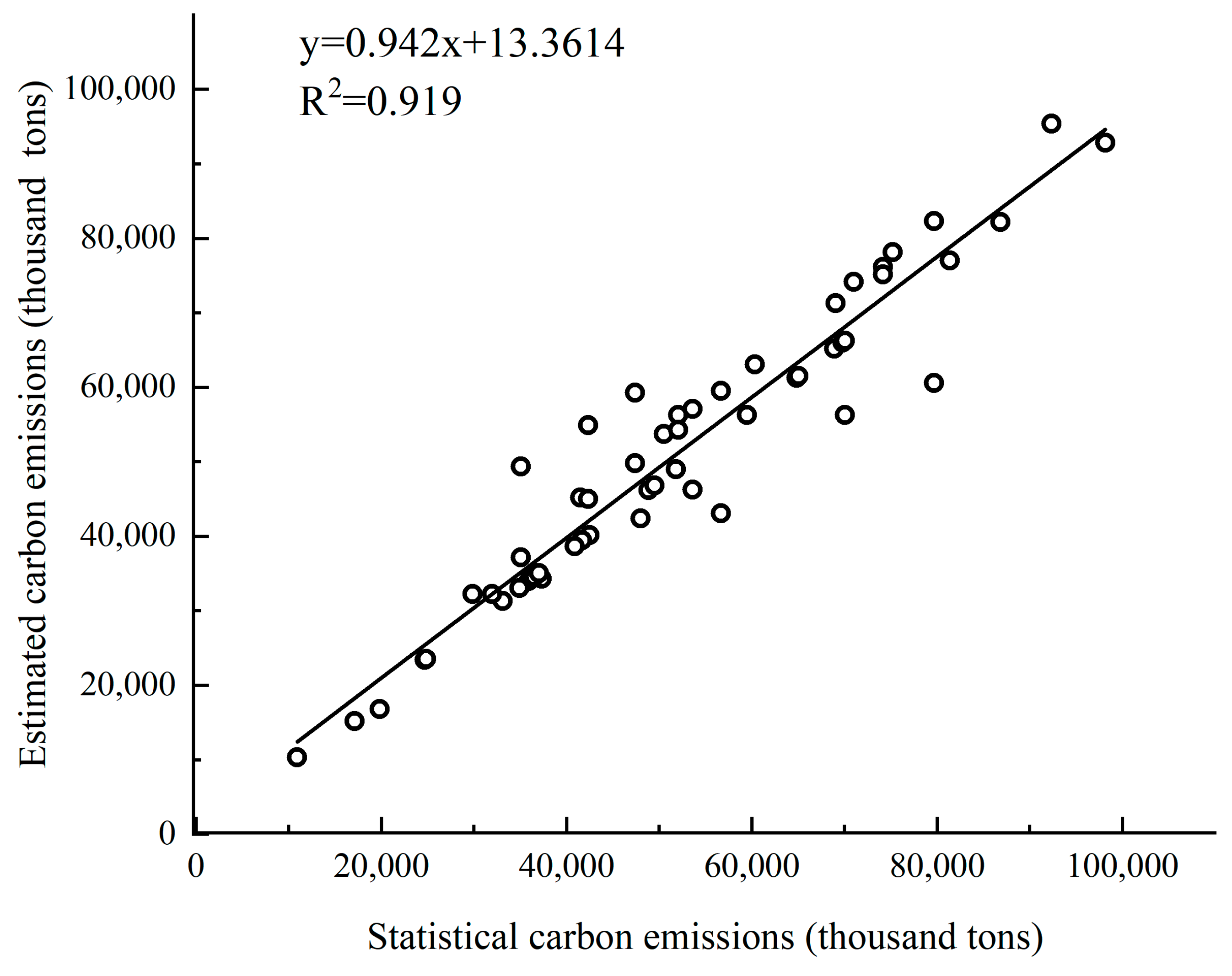
This work builds a linear regression model integrating statistical data with estimated data (Figure 3) in order to further test the validity of the fixed effects model (FE) for estimating carbon emissions from energy consumption. The most straightforward and fundamental supervised learning model in machine learning is the linear regression (LR) model. Finding the line of best fit to best fit the model given a set number of data points is the primary goal of LR [48]. According to the results, there was no significant overestimation or underestimation, and the relationship between the estimated carbon emissions and statistical carbon emissions, as determined by the linear regression model, was expressed as y = 0.942x + 13.3614 with R2 = 0.919. This suggests that the fixed effects model’s (FE) estimation was very good.
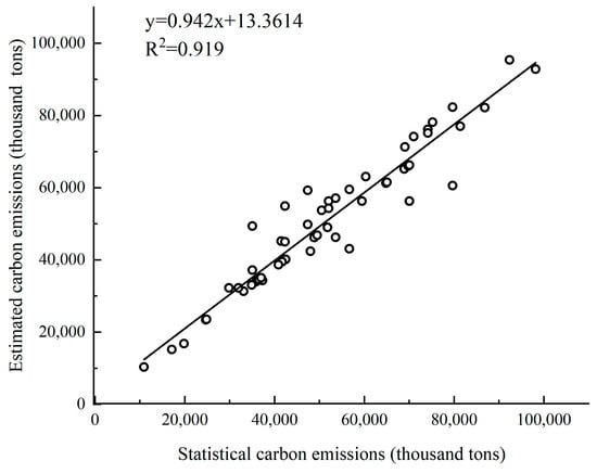
Figure 3.
Scatter plot of the linear regression model.
4.2. The PRD’s Temporal and Spatial Distribution of Carbon Emissions from Energy Consumption
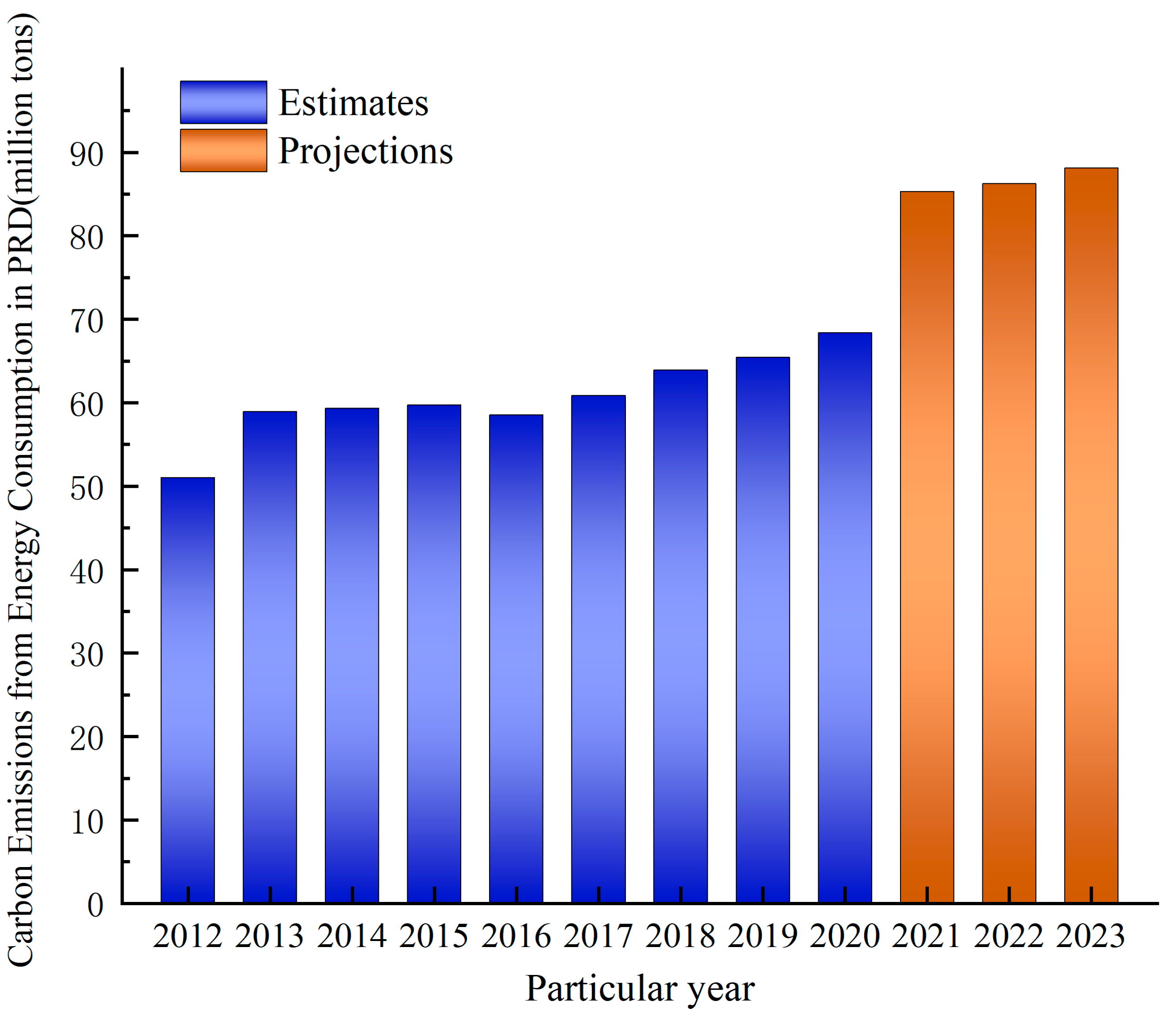
In this study, the fixed effects model estimated the carbon emissions from energy consumption in the PRD from 2012 to 2020 and predicted the emissions for 2021–2023 using municipal nighttime light luminance data (Figure 4). The estimates showed an overall upward trend in carbon emissions, with a stable but slight increase, especially during the period 2015–2019. The carbon emissions reached their highest value during the estimation period in 2019. This result is consistent with the findings of Yu et al. [49]. The prediction results showed that carbon emissions began to rise rapidly in 2020 and reached a new high in 2021, after which they remained at a high level.
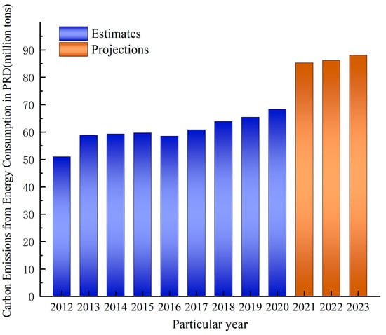
Figure 4.
Two-dimensional bar chart of carbon consumption in the Pearl River Delta (PRD).
Despite some degree of energy efficiency gains, overall carbon emissions have increased, suggesting that the efficiency gains have not been strong enough to offset the growth in emissions from increased economic and construction activity. Future projected data emphasize the need for more stringent policies and advanced technologies to control the growth of carbon emissions and promote a low-carbon economy and sustainable development [50]. Long-term strategies to promote green buildings, renewable energy, and energy-efficient technologies are needed to reduce carbon emissions and improve environmental quality [51].
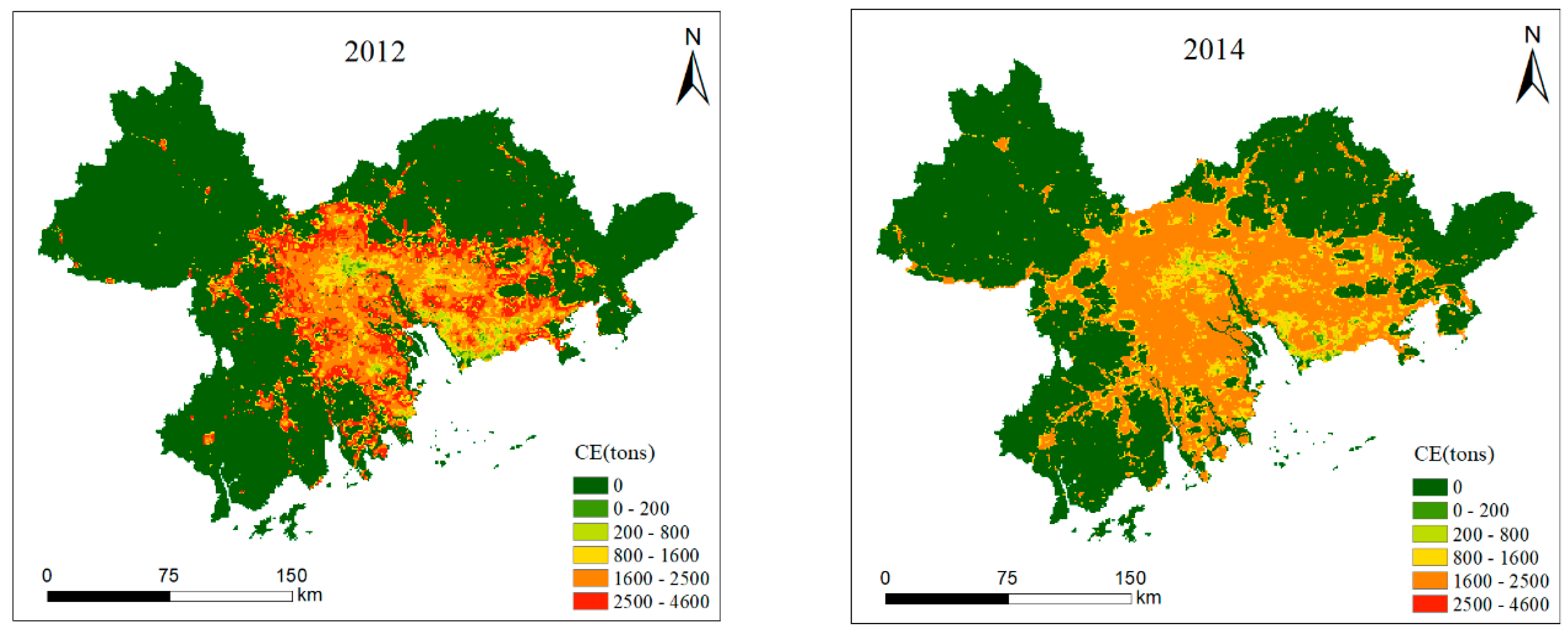
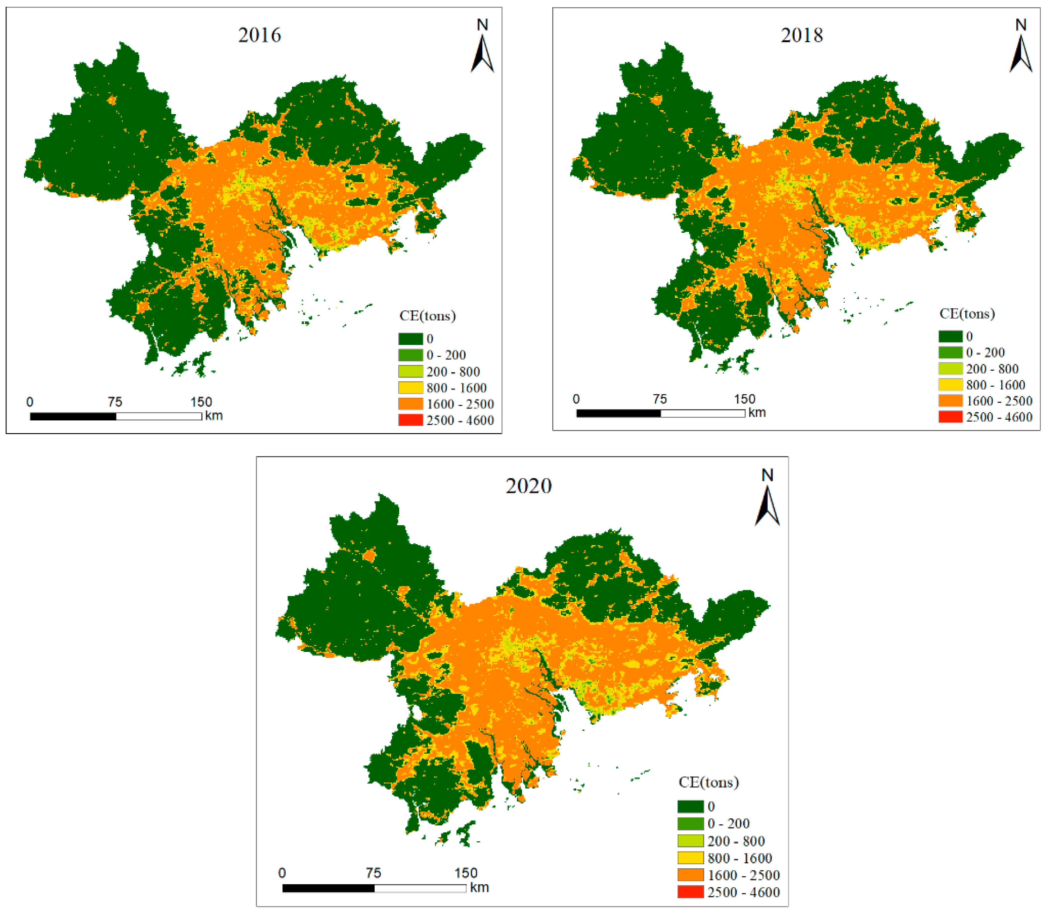
This work applied NPP-VIIRS-like nighttime lighting data to examine carbon emissions (CE) at the 1 km grid size in the territory of the Pearl River Delta (PRD) between 2012 and 2020 (Figure 5). The findings indicate that carbon emissions are unevenly distributed throughout space, being “high in the middle and low at both ends”. High emissions in 2012 were centered in the PRD’s center and west, as indicated by the orange and red areas, while the east and south had lower emissions, shown in green. By 2014, the high-emission area expanded outward, especially around the central city and the Pearl River Estuary. This trend continued in 2016 and 2018, with high emissions remaining in the center and west. However, by 2020, the amount of carbon emissions significantly decreased, especially in traditionally high-emission regions, shifting to green. This decrease may be due to effective environmental policies, the increased use of clean energy, and industrial upgrading. Overall, while some areas saw increased emissions from 2012 to 2018, by 2020, the overall carbon emissions had decreased significantly.

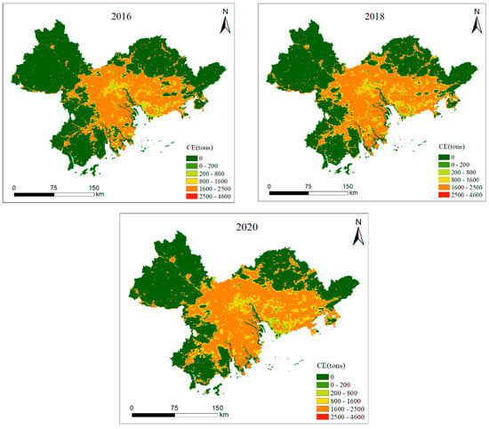
Figure 5.
Estimated carbon emissions at the 1 km grid scale in 2012–2020.
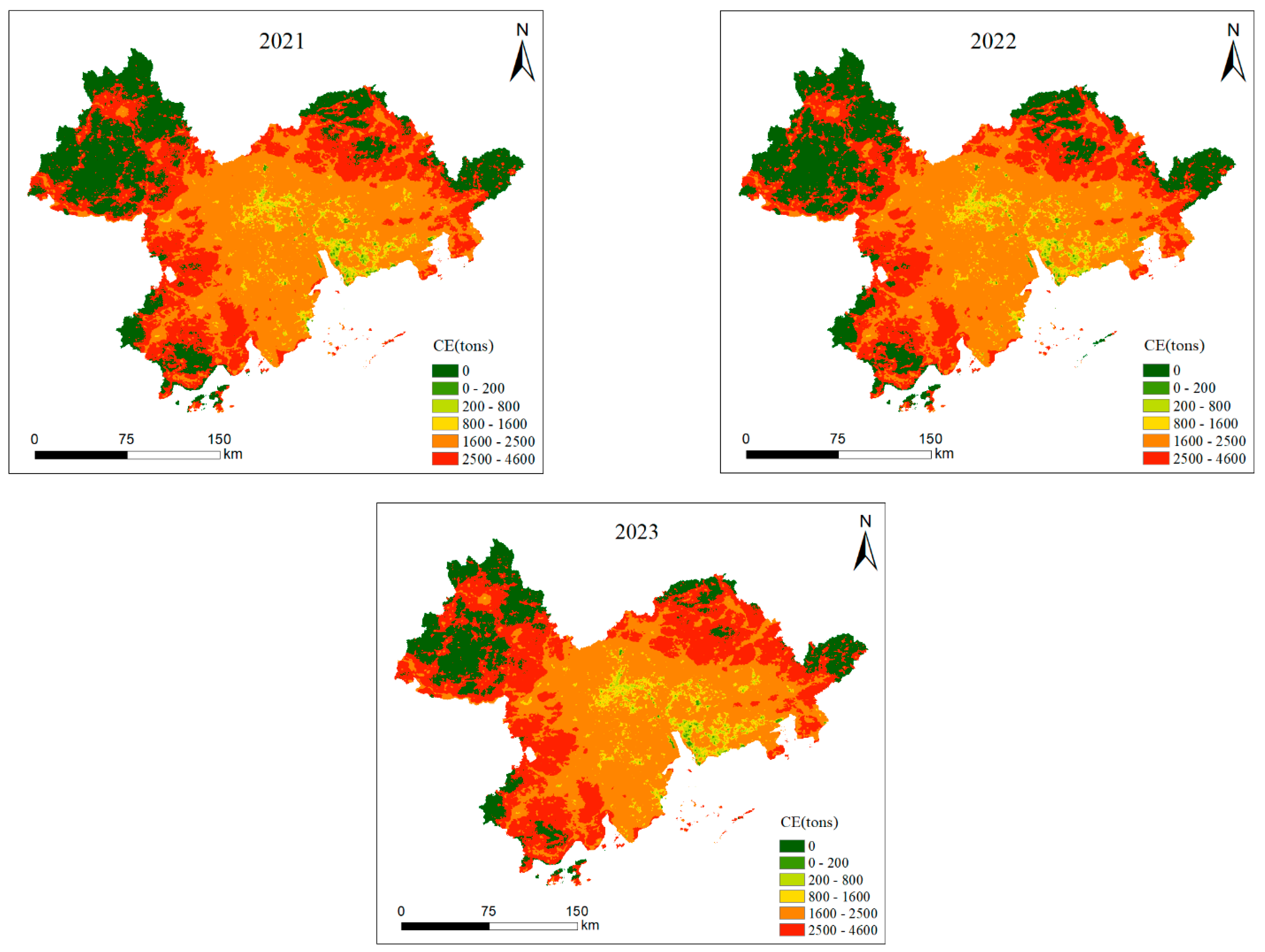
This study projected the carbon emissions in the PRD region at the 1 km raster scale from 2021 to 2023 using data on nighttime lighting (Figure 6). In 2021, central areas and those around the Pearl River Estuary showed high emissions, indicated by orange to red colors. Compared to 2020, high-emission areas increased, especially in the eastern PRD and central cities. By 2022, these areas expanded further, particularly in the northeastern and southwestern Pearl River Estuary, suggesting increased industrial activities or less efficient energy consumption. In 2023, high-emission areas remained in the center and east but contracted slightly in the north and west, with more green areas indicating progress in energy consumption or emission control. With a resurgence in heavy industry, manufacturing, and logistics following COVID-19, the economic recovery was probably the reason behind the rise in carbon emissions between 2021 and 2022. The slight decrease from 2022 to 2023 may be due to enhanced environmental protection measures, optimized energy structures (e.g., more renewable energy), and the restructuring of high-carbon industries.
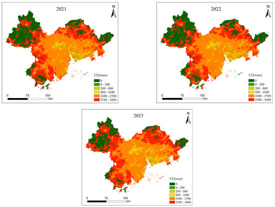
Figure 6.
Carbon emission forecast at 1 km grid scale in 2021–2023.
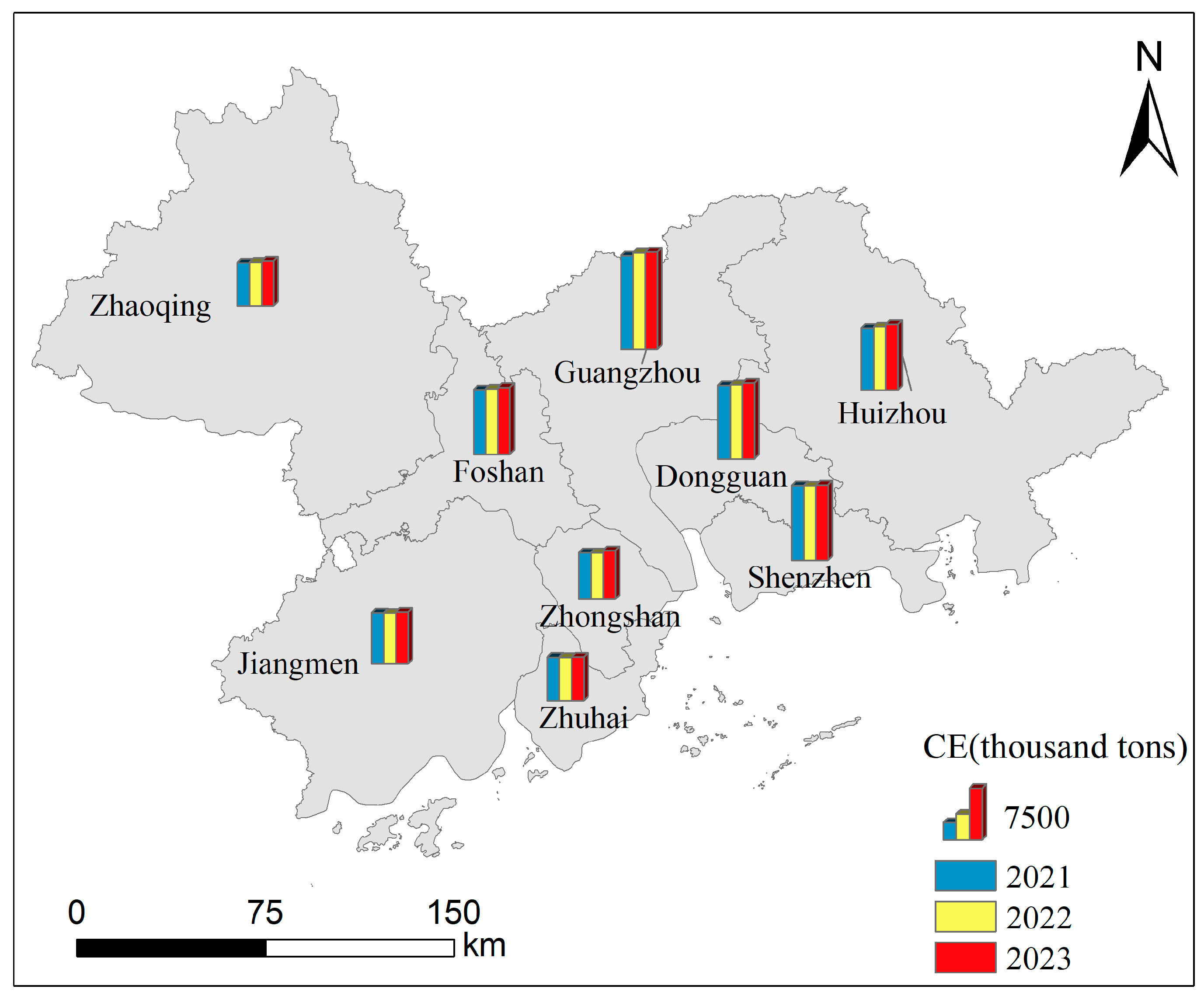
The predicted carbon emissions from energy consumption in the PRD for the years 2021–2023 are displayed in Figure 7 as a column distribution. The findings suggest that, during the years 2021–2023, the PRD city cluster’s carbon emissions generally exhibited a pattern of increasing year over year. Shenzhen, Dongguan, and Shenzhen had the most carbon emissions, followed in third place by Foshan and Huizhou. Wang et al. summarized that the growth rate of carbon emissions in the cities of Guangzhou, Zhuhai, Foshan, and Dongguan is significant relative to the growth rate of the economic expansion in 2015–2020 [52]. This conclusion is consistent with the results of this study. The cities Jiangmen, Zhaoqing, Zhuhai, and Zhongshan had the lowest carbon emissions. Guangzhou, Dongguan, and Shenzhen had the fastest rates of growth, whereas Zhaoqing, Zhuhai, and Zhongshan had slower rates of growth and were in a stable state.
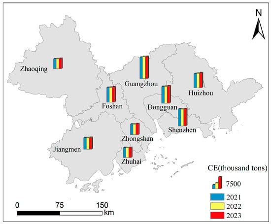
Figure 7.
Forecast of energy consumption in PRD city.
The Pearl River Delta (PRD), home to developed cities like Shenzhen, Dongguan, and Guangzhou, is a major source of carbon emissions from industrial activity, particularly heavy industry and manufacturing. Rising productivity is accompanied by rising carbon emissions. These heavily populated cities, which mostly rely on fossil fuels like coal and oil, consume enormous amounts of energy. Shenzhen is a major economic hub with considerable indirect carbon emissions, mostly from transportation and power. In the Pearl River Delta (PRD), urban development and rapid urbanization cause ecological changes that raise carbon emissions. Huizhou and Foshan are significant industrial hubs with substantial carbon emissions and energy consumption. These two cities are major centers for transportation, thus their logistics and transportation-related activities also contribute significantly to carbon emissions. Zhaoqing and Jiangmen have fewer industrial activities and lower carbon emissions, focusing mainly on light industry and services. Zhuhai and Zhongshan, despite their industrial development, have a larger share of high-tech and modern service industries and lower carbon emission intensity. These cities have implemented environmental protection policies, promoted clean energy and energy efficiency, and effectively controlled the growth of carbon emissions by optimizing the urban layout and strengthening environmental management [53,54].
4.3. Time Trend Analysis of Carbon Emissions from Energy Consumption in the PRD
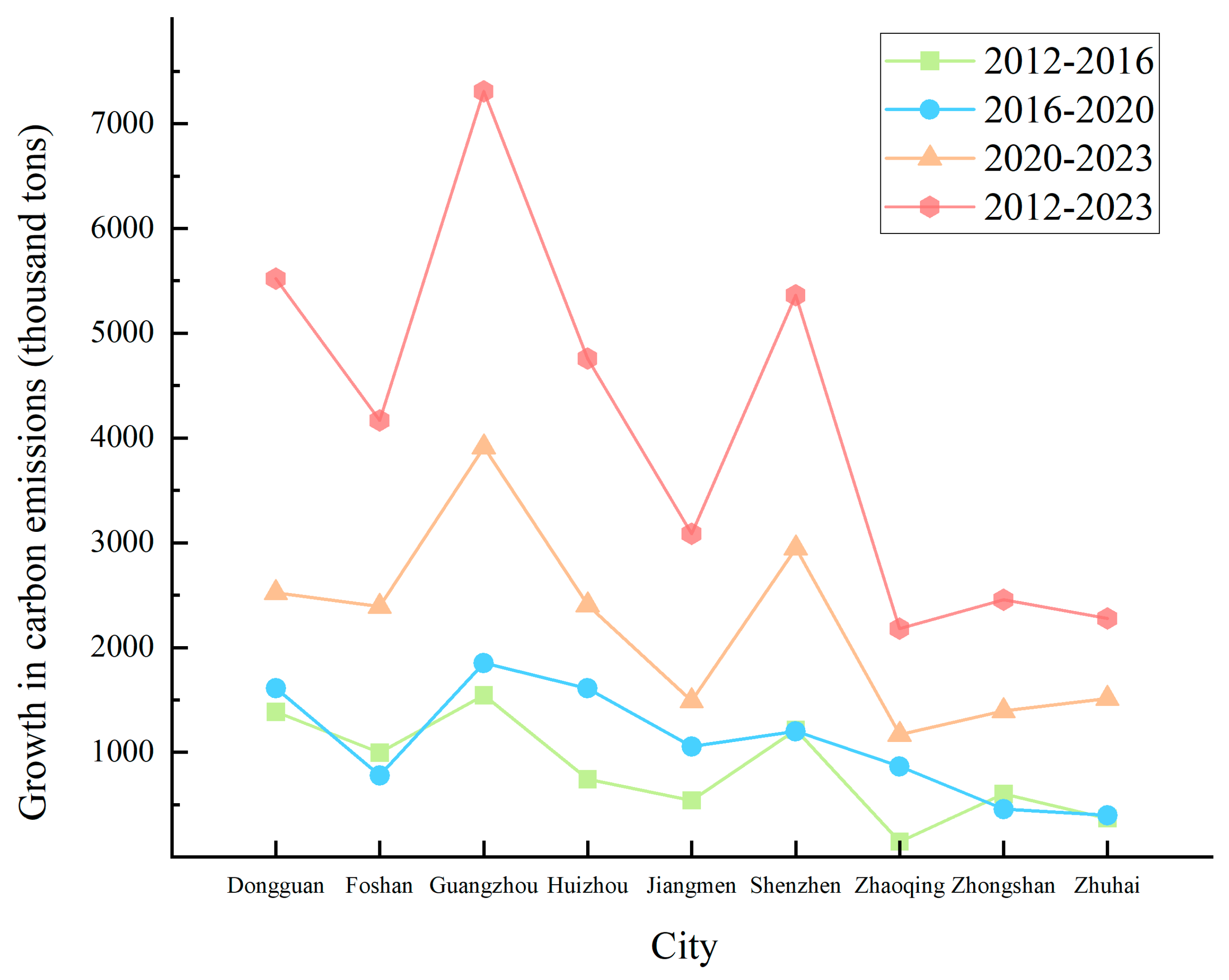
Using anticipated and estimated data, this study examined the temporal trend of carbon emissions in the PRD (Figure 8). In the first-time interval (2012–2016), the growth trend of carbon emissions was relatively flat and similar for all major cities, including Shenzhen and Guangzhou, suggesting a relatively consistent pattern of growth in construction and economic activities across the major cities during that time period. However, in the subsequent time periods (2016–2020 and 2020–2023), the growth of carbon emissions in Shenzhen and Guangzhou accelerated significantly, showing an outstanding growth trend. This may be due to the rapid urbanization, industrialization processes, and accelerated economic activities in Shenzhen and Guangzhou in that time period [55]. The charts do not show a significant difference between the growth of Shenzhen and Guangzhou in the first two time periods, possibly because the growth patterns in the first two time periods were more consistent, while the rapid growth in the latter two time periods reflects more drastic changes in economic and construction activities. In addition, the carbon emissions in Shenzhen and Guangzhou rose sharply in 2020–2023, during the post-epidemic economic recovery, peaking in 2023, suggesting that emission control policies and technological advances were not fully effective [56]. Dongguan and Zhongshan also saw increases, but to a lesser extent. Overall, from 2012 to 2023, Shenzhen and Guangzhou experienced significant growth in their carbon emissions due to their economic and industrial development, especially during the post-epidemic period. In contrast, Zhaoqing and Jiangmen had relatively stable emissions, likely due to their lower industrial activity and reliance on agriculture and services, which have lower carbon emissions.
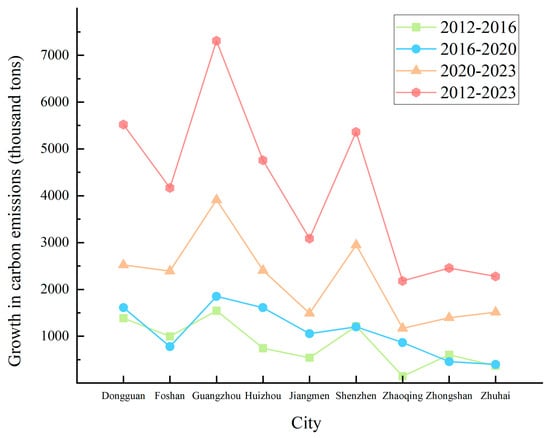
Figure 8.
Growth trend of energy consumption and carbon emission in the Pearl River Delta.
This study examined the spatial distribution of the carbon emission growth from energy consumption in the PRD over four periods. As shown in Figure 9, carbon emission growth was “high in the middle and low at both ends”. From 2012 to 2016, high growth was mainly in central PRD, especially Guangzhou, with medium growth in the central and eastern parts, and low growth in northern cities like Zhaoqing and southern cities like Jiangmen and Zhuhai. From 2016 to 2020, high growth expanded to Dongguan and Huizhou, indicating increased industrial and economic activities. From 2020 to 2023, high growth was observed mainly in central and eastern cities like Guangzhou, Dongguan, and Shenzhen, but densities slightly decreased due to stricter environmental policies and technological improvements. Xu et al. found that Guangzhou and Shenzhen are the cities with the largest carbon emissions in the PRD [57], which confirms the results of this study. Medium growth became more dispersed, located in the southern, central, and northern parts, while low growth occured mainly in Zhuhai. Overall, between 2012 and 2023, the center region continued to see high growth, the eastern region and the areas around high-growth zones experienced medium growth, and the southern, middle, and northern regions—including Zhaoqing, Foshan, and Jiangmen—saw low growth.
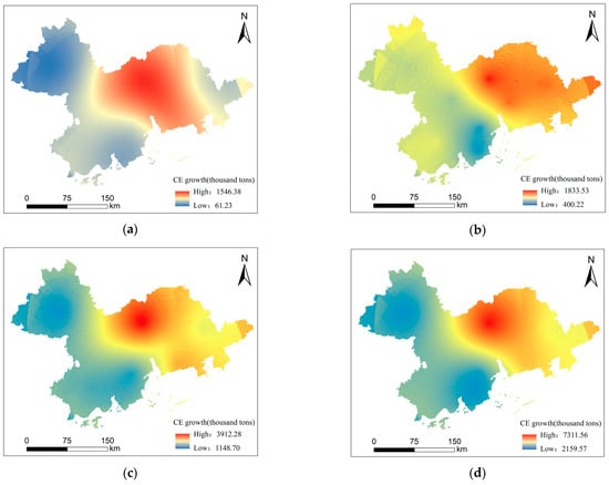
Figure 9.
(a–d) shows the spatial distribution plots of the growth trends of energy consumption in the Pearl River Delta in 2012–2016, 2016–2020, 2020–2023 and 2012–2023, respectively.
Guangzhou, Shenzhen, and Dongguan are major economic and industrial centers in the PRD, experiencing significant carbon emissions growth due to intensive industrial activities and rapid urbanization [58]. Large populations and busy transportation systems also contribute to high emissions. The post-SARS economic recovery (2020–2023) further increased industrial and economic activities, keeping carbon emissions growth high, despite environmental measures. To control and reduce carbon emissions, it is crucial to strengthen environmental policies, especially in high-emission regions. Investing in and using cleaner energy, reducing the reliance on fossil fuels, enhancing energy efficiency through technological improvements and management optimization, and reducing unnecessary energy wastage are essential steps. By taking these steps, the PRD region will be able to successfully regulate carbon emissions while preserving economic growth and pursuing sustainable development [59].
4.4. An Analysis of the Pearl River Delta’s (PRD) Hotspots for Carbon Emissions and Energy Consumption
The spatial clustering of carbon emissions in the Pearl River Delta (PRD) between 2012 and 2020 was determined in this study using a hotspot analysis (Figure 10). The primary hotspot location, as indicated by the results, is the central PRD, indicating extremely high carbon emissions there. From 2012 to 2014, Guangzhou transformed from a sub-hotspot to a hotspot area, with sub-hotspot areas expanding and coldspot areas reducing to just Zhuhai. During 2014–2016, Zhaoqing changed from a sub-hotspot to a coldspot area, while hotspot areas remained stable. From 2016 to 2018, Zhaoqing shifted from a coldspot to a sub-coldspot area, with sub-hotspots expanding to include Huizhou. By 2020, the spatial distribution of hotspots and coldspots was similar to 2018, but hotspots expanded to include Dongguan alongside Guangzhou.
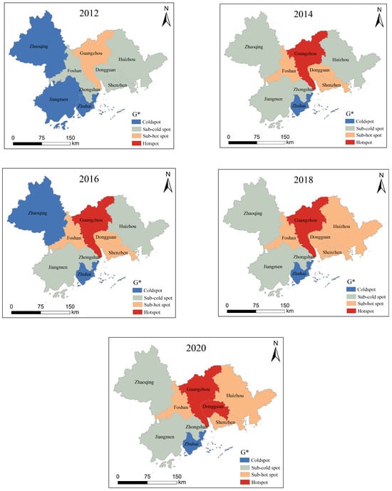
Figure 10.
The spatial aggregation and distribution diagram of coldspots and hotspots of energy consumption and carbon emission in the Pearl River Delta (G* is the local spatial autocorrelation index in spatial statistics used to analyze the region aggregation in geospatial data).
Overall, Guangzhou, Shenzhen, and Foshan have consistently been hotspot areas due to high industrialization, population density, and traffic flow, leading to higher carbon emissions. Zhaoqing and Jiangmen remained coldspot regions, likely due to their low industrial activity, low population density, and higher forest cover. From 2012 to 2020, carbon emission hotspots expanded from Guangzhou and Shenzhen to Foshan and Dongguan, reflecting the spread of economic activities and industrial production [60].
4.5. Analysis of Factors Affecting Carbon Emissions from Energy Consumption in the PRD
In this study, demographic factors, economic factors, technological factors, land area, environmental factors, and energy factors were selected to examine the variables affecting the carbon emissions from energy consumption in the PRD (Table 5). Six variables, namely population size, gross regional product, expenditure on research and development, built-up area, vegetation cover, and energy intensity were utilized to represent demographic, economic, scientific and technological, land area, environmental, and energy factors, respectively, and these six variables were used as explanatory variables; however, in the examination of influential elements, the predicted quantity of the carbon emissions resulting from energy consumption in the PRD served as the dependent variable.

Table 5.
Impact factor data based on statistics.
This research analyzed the elements influencing the emissions of carbon using the OLS, GWR, GTWR, and MGWR models, based on the components that had been identified, and we compared the outcomes to determine which model was the best. As shown in Table 6, the GWR, GTWR, and MGWR models, which include spatial features, outperformed the OLS model. Specifically, the MGWR model had the lowest residual sum of squares (RSS) and AICc, and the highest goodness of fit (R2), indicating it was the best model. This is likely because the MGWR model overcomes the limitations of the OLS model’s global parameters and the fixed spatial scales of the GWR and GTWR models, making it more suitable for data with spatial attributes. This suggests that the elements affecting carbon emissions in the PRD vary across different spatial scales. From Table 6, it can be seen that the population, economy, land area, and energy factors positively impacted carbon emissions, with the economy having the most significant positive effect. Conversely, science and technology, as well as environmental factors, negatively impacted carbon emissions, with science and technology having a more significant negative effect than environmental factors.

Table 6.
Model comparison results.
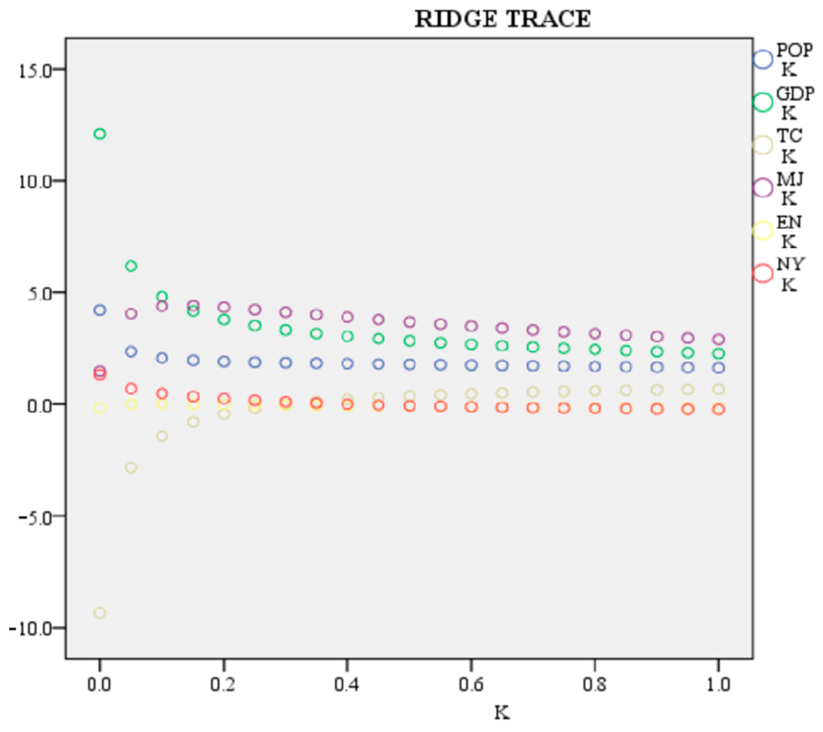
For the three effect factors of economy, science and technology, and energy, as indicated in Table 7, the values of the Variance Inflation Factor (VIF) exceeded the intended threshold of 10 [61], pointing to a significant issue with multicollinearity. Furthermore, statistics and unrealistically high R2 values frequently highlighted the overfitting issues related to multicollinearity [62]. This study extended the MGWR model using the ridge regression technique created by Hoerl and Kennard in 1970 to address the issue of multicollinearity. The procedure chooses a suitable ridge regression coefficient, k, which ought to be the lowest number that yields a reliable approximation. Plotted ridge trace curves served as the basis for determining the value of k in this investigation [63,64]. The ridge trace curve tended to stabilize at k = 0.4, as Figure 11 illustrates. Consequently, in this investigation, the ridge regression was estimated using this value.

Table 7.
The VIF values for each impact factor.
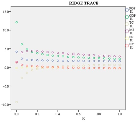
Figure 11.
The ridge trace curve. Note: POP, GDP, TC, MJ, EN and NY denote demographic, economic, scientific and technological, land area, environmental, and energy factors, respectively.
Overall, The MGWR model, extended using ridge regression, had an R2 of 0.903, indicating a good fit (Table 8). At the 1% level, each of the independent variables was significant. The four key factors—population, economy, land area, and energy—showed positive correlations with carbon emissions (CTCE), with regression coefficients of 0.421, 0.891, 0.148, and 0.133, respectively. In contrast, science and technology, and environmental factors were negatively correlated with CTCE, with coefficients of −0.930 and −0.117. Population growth significantly increased carbon emissions due to a higher energy demand from residential and industrial activities in the densely populated PRD region. Economic growth in this hub of manufacturing and services leads to increased industrial production, energy consumption, and transportation, all of which have a major beneficial impact on emissions. Technological advancements significantly reduce carbon emissions by improving energy efficiency, developing renewable energy, and enhancing production processes. Wang et al. similarly confirmed that demographic factors contribute to the growth of carbon emissions from energy consumption in the PRD and that technological factors could help to reduce carbon emissions [65]. Land expansion, however, increases emissions due to urban sprawl and development activities that raise the energy demand and reduce forests and green spaces, weakening natural carbon sinks. Good environmental management and conservation measures, such as afforestation and ecological restoration, reduce carbon emissions. Energy consumption remains a major contributor to emissions, as the PRD’s high energy demand is still largely met by traditional fossil fuels, despite some use of renewable energy. These findings suggest that policymakers in the PRD region should focus on improving energy efficiency, promoting technological innovation, planning land use rationally, optimizing the energy mix, and enhancing environmental protection measures to reduce carbon emissions.

Table 8.
Results of the MGWR model: ridge regression (K = 0.4).
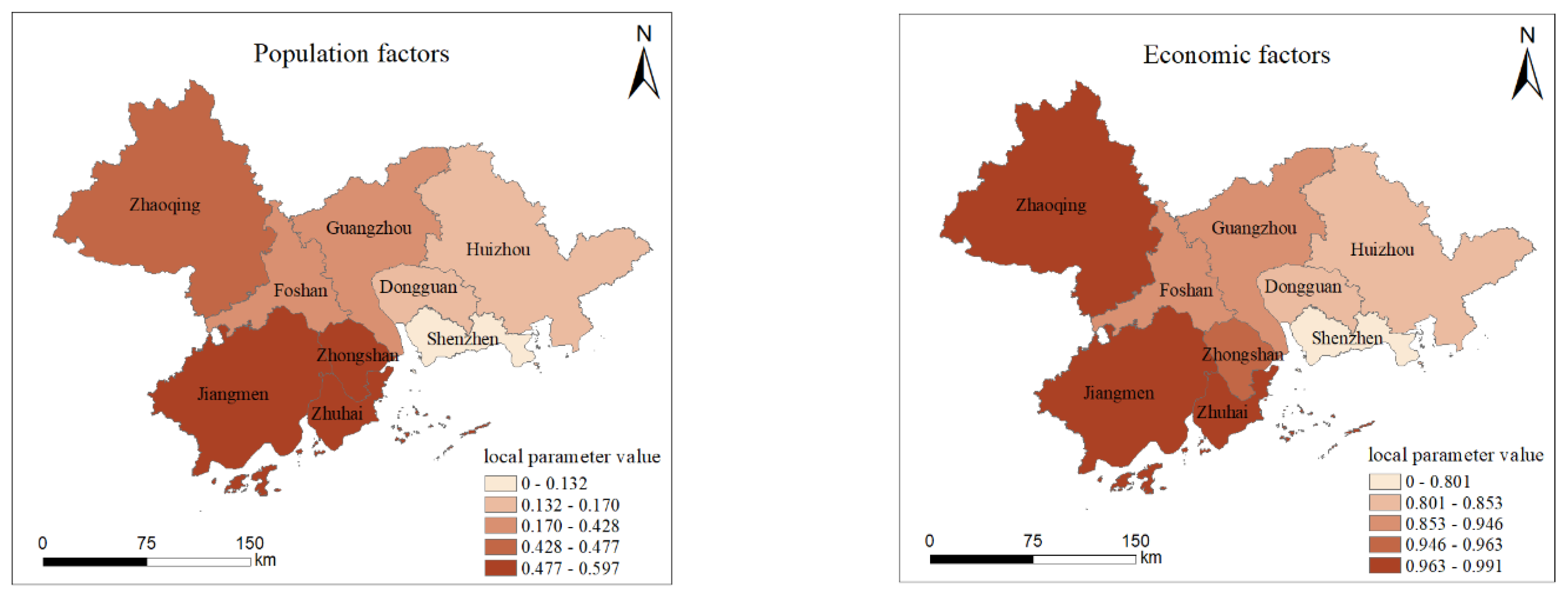
Figure 12 illustrates the spatial change patterns of the localized parameters of the population, economics, science and technology, land area, environment, and energy variables of the carbon emissions resulting from energy consumption in PRD prefectures. The following aspects were examined in more detail:
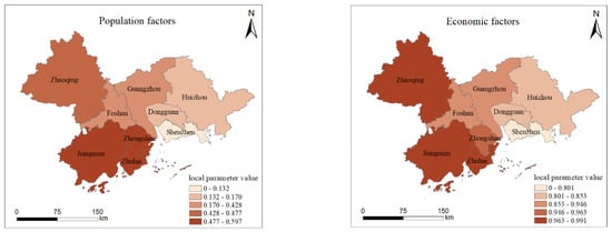
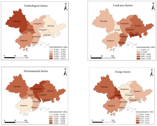
Figure 12.
Spatial distribution of factors influencing carbon emissions of energy consumption in the Pearl River Delta cities from 2012 to 2020.
- (1)
- In the southern PRD cities, the population factor positively affected carbon emissions more than other factors, mainly due to the fact that these cities are in the stage of rapid urbanization and industrialization, with relatively imperfect infrastructures and the insufficient application of environmental protection policies and technologies. The lesser impact on the eastern cities, especially Shenzhen, is due to the fact that these cities have already achieved a higher level of economic development, with well-developed infrastructures and advanced environmental protection technologies, as well as higher rates of public transport usage and energy-efficient buildings. These elements work together to explain why different cities experience different effects of population expansion on carbon emissions.
- (2)
- Economic considerations had a moderate impact in the east and a large one in the west on the carbon emissions in the PRD region, mainly due to differences in the economic structure, energy consumption efficiency, environmental protection policies and transport infrastructure. The economic growth of western cities such as Zhaoqing, Jiangmen, and Zhuhai relies mainly on traditional manufacturing industries and infrastructure development with high carbon emissions, while eastern cities such as Shenzhen and Dongguan rely on high-tech and service industries, more efficient energy consumption, stricter environmental protection policies, and better transportation systems, which significantly reduce the results of economic activity on carbon emissions. These factors work together to lead to notable regional variations in the relationship between economic expansion and carbon emissions.
- (3)
- Because of the considerable advancements in the application of science and technology as well as the notable decrease in emissions brought about by Zhaoqing’s extensive technological transformation, the science and technology element had the largest negative influence on carbon emissions. The impact on eastern PRD cities, such as Dongguan, Huizhou, and Shenzhen, was smaller because these cities already have higher levels of technology application, diversified industrial structures, and high-tech economic structures, making the marginal abatement effect of technological progress on carbon emissions relatively weak. These differences between different regions reflect the role and effect of science and technology in different stages of development and economic structures.
- (4)
- In the PRD region, the land area factor’s overall beneficial effect on carbon emissions was less pronounced, but it had a greater impact on the eastern region (especially Shenzhen), due to the fact that the high-density urbanization, highly efficient public transport system, intensive industrial structure and strict environmental protection policies in the eastern region make the expansion of land area directly affect the energy demand and carbon emissions. On the other hand, in the western region, land area expansion had less impact on carbon emissions, due to low-density urbanization, traditional industrial structure, relatively lax environmental policies, and less advanced infrastructure. These differences reflect the various ways that land use influences carbon emissions in different cities in the development process.
- (5)
- Environmental factors affecting carbon emissions vary based on the geographical location, industrial structure, and transportation conditions. All things considered, the PRD region’s carbon emissions were negatively impacted by these factors to a minor extent; however, the impact was greatest in the eastern region, namely Guangzhou City, and least in the western region, specifically Jiangmen City. Guangzhou, as an important economic center, has high urbanization, dense buildings, and limited green space. In this high-density urban environment, the limited vegetation cover can only absorb a small portion of the significant carbon emissions from industry and transportation. However, recent efforts to increase urban green space in Guangzhou have made environmental factors more significant in reducing emissions. In contrast, Jiangmen’s carbon emissions were relatively low and decentralized, mainly from agriculture and small-scale industry. The high vegetation cover in Jiangmen already absorbs a significant amount of carbon, so further increasing vegetation has a limited effect on reducing emissions.
- (6)
- The energy factor significantly impacted the carbon emissions in Zhaoqing and Foshan, due to their heavy industry and manufacturing sectors, high fossil fuel use, low energy efficiency, poor implementation of environmental policies and technologies, decentralized urban layout, and lagging infrastructure. These factors collectively make energy consumption’s positive impact on carbon emissions particularly pronounced in these cities. Conversely, in cities like Shenzhen and Guangzhou, the impact of energy factors on carbon emissions was relatively small because of their high-tech and service industries, high use of clean energy, efficient energy utilization, stringent environmental policies, and well-developed infrastructure.
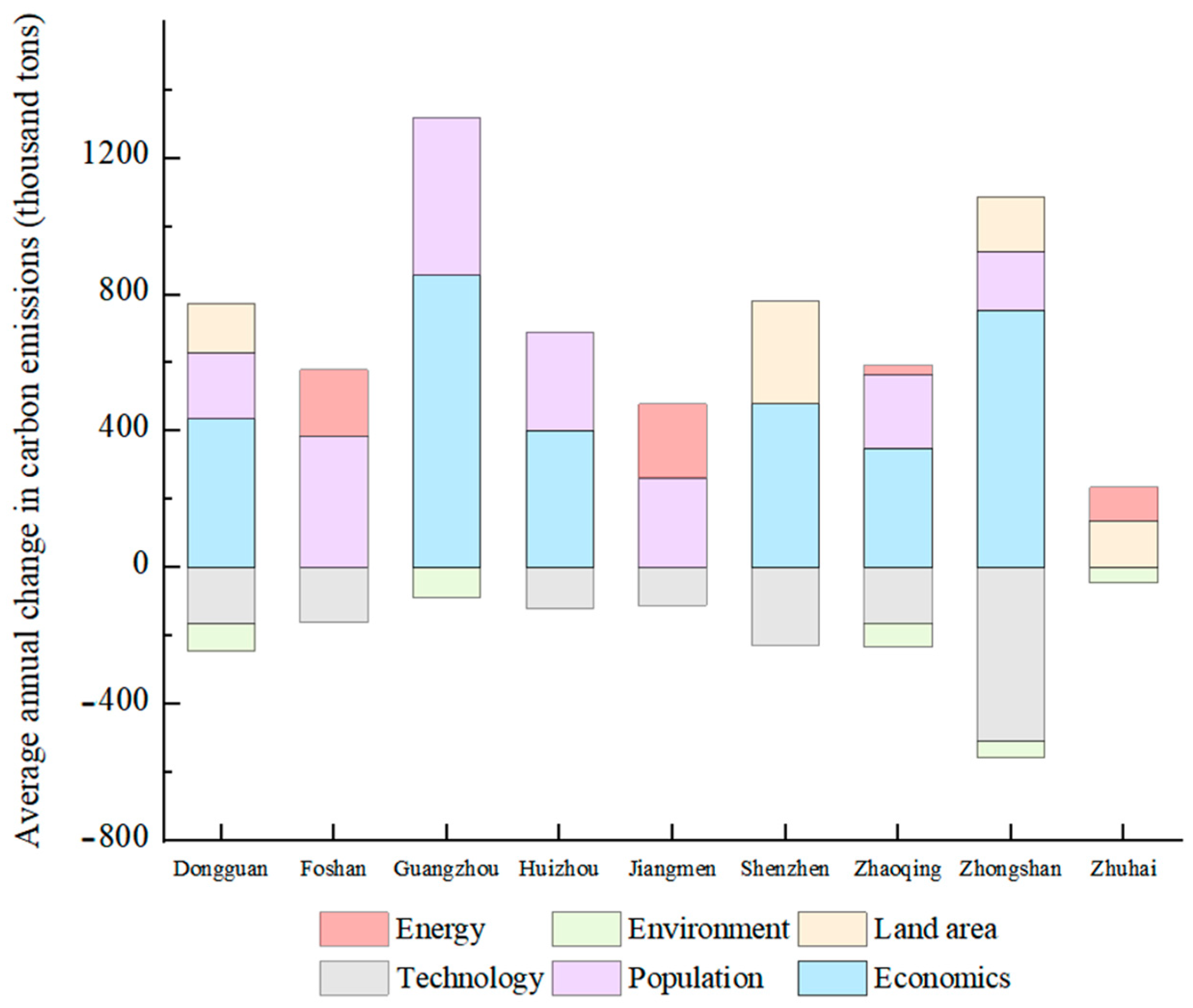
There are variations in the degree and patterns of various influencing elements because of the unequal spatial and temporal distribution of carbon emissions from energy consumption at the municipal level in the PRD. Consequently, from 2012 to 2020, this study examined the impact of a number of variables on the average yearly change in the carbon emissions from energy consumption at the municipal level in the PRD (Figure 13). The results show that demographic and economic factors were the main drivers of carbon emission growth in the PRD region, and that technological and scientific factors presented significant emission reduction advantages in the 2012–2020 period. For example, demographic and economic factors led to an average annual growth of 4,631,700 tons and 8,576,040 tons of carbon emissions in Guangzhou City, respectively, while technological factors led to an average annual reduction of 5,089,870 tons of carbon emissions in Zhongshan City.
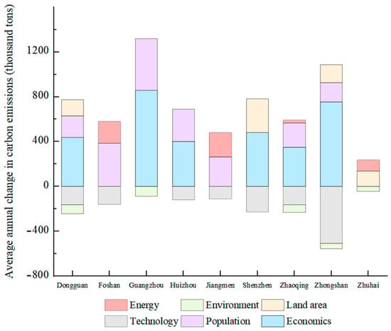
Figure 13.
Influence of each factor on the annual average change of energy consumption and carbon emissions in the PRD city.
Carbon emissions in different cities are influenced by various factors [66]. In Guangzhou and Zhongshan, economic growth, manufacturing and service industry expansion, and infrastructure development drove up the emissions. Zhaoqing, with low economic development and slow industrialization, saw minimal impact from economic activities. Population growth significantly increased the emissions in densely populated cities like Foshan and Guangzhou, where urban expansion and a higher energy demand play major roles [67]. Energy consumption impacted Foshan and Jiangmen due to their heavy industry and reliance on high carbon-emitting energy types. Scientific and technological progress reduced the emissions in Shenzhen and Zhongshan, where high-tech industries and environmental technologies improve energy efficiency. Environmental factors significantly reduced the emissions in Guangzhou, Dongguan, and Zhaoqing through investments in environmental protection and greening, which enhance carbon absorption. Land area expansion increased the emissions in Shenzhen and Zhuhai, where rapid urbanization and high-density buildings drive up carbon output. These differences highlight the need for cities to develop targeted carbon emission control strategies, optimize economic structures, promote energy-saving technologies, and strengthen environmental governance to effectively control emissions [68].
5. Discussion
5.1. Applicability of Panel Model-Based Carbon Emission Estimation for Energy Consumption
This study employed a panel unit root test, panel data integrality and covariance test methods, based on provincial energy carbon emissions and nighttime light brightness values, to investigate the feasibility of a long-term association between carbon emissions and DN values and to verify the smoothness of the first-order difference series of the variables connected to carbon emissions. To ascertain whether the panel data—multidimensional data spanning time and individuals—have a unit root, or whether the data are smooth, one can use the panel unit root test. The panel unit root test offers several benefits over the conventional time series unit root test, including increased test efficacy, the ability to handle heterogeneity, the ability to control for individual effect, the availability of a range of tests, and the ability to handle cross-individual dependence. To find out if there is a long-term stable link between several time series in panel data, cointegration tests are utilized. The panel data cointegration test offers several test techniques, improves test efficacy, and can handle individual heterogeneity when compared to the single time series cointegration test. At the same time, the panel data cointegration test allows the cointegration vectors of different individuals to be heterogeneous, which can more accurately reflect the complexity of the actual economic relationships, and the panel data cointegration analysis improves the estimation efficiency and parameter stability by estimating the cointegration relationships of multiple individuals together. The panel data cointegration analysis allows the introduction of an error correction mechanism (ECM) into the panel data model, which dynamically adjusts the short-term deviations and achieves the tracking of the long-run equilibrium relationship.
5.2. Uncertainty Analysis of Influencing Factors
In order to determine the optimal MGWR model for examining the variables influencing energy carbon emissions in the PRD, this study evaluated model outputs. Multi-scale geographically weighted regression (MGWR) allows each independent variable to vary at different spatial scales, capturing spatial data heterogeneity more accurately. Initially, the study considered demographic, economic, technological, land area, environmental, and energy factors, but did not include climatic factors. Climatic factors can directly or indirectly affect carbon emissions. For example, extreme high temperatures increase air conditioning use, raising the electricity demand and carbon emissions, while extreme low temperatures increase the heating demand. Changes in precipitation patterns can impact hydroelectric power generation, with droughts reducing hydropower and increasing reliance on fossil fuels, thus raising carbon emissions. Wind and solar radiation changes can affect the efficiency of wind and solar power generation, with climate change potentially causing instability in these renewable energy sources. Therefore, the study added climate factors, including annual precipitation, average annual temperature, and annual sunshine hours (Table 9).

Table 9.
Shows data on climate factors based on statistics.
Then, the MGWR model was employed to examine the variables affecting the PRD’s carbon emissions. The results in Table 10 show strong explanatory power (R2 = 0.931) and a small fitting error (RSS = 5.609), proving that the model can adequately account for the variations in carbon emissions caused by municipal energy consumption. Higher numbers indicated a greater fit in the log-likelihood value, which was used to evaluate the model fit. Model selection was based on AICc and AIC values, where lower values denoted a better fit. The average yearly temperature, annual sunshine hours, and annual precipitation all had regression coefficients on carbon emissions of 0.109, 0.168, and 0.013, respectively, indicating that these variables had no effect on carbon emissions in the PRD. The p-values for average annual temperature and annual sunshine hours were less than 0.01, indicating statistical significance at the 1% level. However, the p-value for annual precipitation was greater than 0.05, indicating it does not significantly affect carbon emissions.

Table 10.
Results of the analysis of the MGWR model.
This study summarizes the above issues; the reason for this phenomenon may be that carbon emissions mainly come from industry, transportation and energy, and these areas do not depend much on precipitation, which affects hydropower generation and agriculture, but these indirect impacts may be counteracted by other factors: for example, when precipitation varies, the power companies may adjust their energy mix to use more fossil fuel generation to make up for the shortfall in hydropower generation, thereby making the effect of precipitation less pronounced. Precipitation affects carbon emissions differently in different regions, which is difficult to reflect in the overall model. An insufficient data sample size or time span affects the accuracy of a statistical analysis. The impact of precipitation may be obscured by other dominant factors, such as energy consumption, economic activity, etc., which have a greater influence on carbon emissions. As a result, additional research might be conducted to extend the sample size and time period, enhance the data quality, guarantee data accuracy and completeness, and remove outliers and missing values. An examination of subregions may also be taken into consideration in order to account for regional heterogeneity.
5.3. Research Limitations
There are three issues with this study that need to be resolved in subsequent research. First, the results of this study may not be accurate because it only used data on nighttime light to estimate carbon emissions, and newer LED lighting technologies (such as those used in Shenzhen) emit light in a range of colors that cannot be fully detected by the NPP-VIIRS sensors, which may lead to the underestimation of nighttime light data and the associated carbon emissions [69]. The limitations of NPP-VIIRS in detecting LED lighting transitions in Shenzhen can be addressed by considering alternative data sources and technologies. Alternative datasets include Landsat and Sentinel-2 high-resolution optical imagery, International Space Station nighttime imagery (for a broader spectral range), and ground-based sensors or drones (for detailed local monitoring). Hyperspectral imaging tools, like Hyperion, capture a wider range of optical frequencies. Combining these data sources improves the accuracy of capturing the nighttime light changes brought about by new lighting technologies [34]. Future research can incorporate data from other remote sensing sources, such as digital elevation models, vegetation indices, land-use data, and carbon satellite data, which can also estimate carbon emissions resulting from energy consumption [70]. Second, this study only considered the environmental impact of CO2 and ignored other pollutants such as PM2.5, sulfur dioxide and carbon monoxide. Future research can examine the effectiveness of reducing pollution and greenhouse gas emissions to create synergistic indicators, evaluate the effects of co-control on the economy or public health, and run scenario assessments under various policy scenarios. Lastly, because changes in land use and urban land expansion frequently cross jurisdictional boundaries [71], this study may have subjectivity issues because it solely examined municipal administrative boundaries in the PRD. Consequently, a multi-modal and multi-scale characterization of the region ought to serve as the foundation for future research [72], and by merging the energy consumption of separated sectors, it may also investigate the temporal and spatial distribution patterns of carbon emissions and the effect mechanisms at the horizontal fine-grained industrial level.
6. Conclusions
In this study, we first used the panel unit root test based on provincial carbon emissions from energy consumption and nighttime illumination brightness values to confirm the smoothness of the first-order difference series of carbon emission-related variables. Next, we used the panel data cointegration test to examine the long-term link between carbon emissions and DN values. In the Pearl River Delta (PRD), municipal-level carbon emissions are estimated and anticipated using a fixed effects model that characterizes both temporal and spatial changes. Lastly, the method by which various factors influence carbon emissions was revealed using the MGWR model. The primary findings are: (1) Carbon emissions and SDN have a long-term link, and the variables associated with carbon emissions have smooth first-order difference series. (2) The fixed effects model (FE) estimates well without serious overestimation or underestimation. Geographically, from 2012 to 2020, the PRD’s carbon emissions were “high in the middle and low at the ends”, with the central and eastern regions of the PRD experiencing the majority of the high emission zones in 2021–2023. Over time, high carbon emission growth from 2012 to 2023 was concentrated in the eastern PRD, with middle values in the eastern part and edges of high value zones, and low values in southern, central, and northern PRD cities like Zhaoqing, Foshan, and Jiangmen. The carbon emission hotspot area gradually expanded from 2012 to 2020. (3) The MGWR model has the best fitting effect. Population, economy, land area, and energy factors positively affect carbon emissions, with economic factors being the most significant. Conversely, science and technology and environmental factors negatively affect carbon emissions, with science and technology having a more significant negative effect than environmental factors. This study provides carbon emission monitoring methods and data for China’s response to climate change, as well as a scientific reference for the optimization of China’s regional energy-saving and emission reduction paths and the realization of the dual-carbon strategy.
Author Contributions
Conceptualization, M.S. and Y.W.; methodology, M.S.; software, M.S.; validation, M.S., Y.W. and Y.H.; formal analysis, Y.J.; investigation, Y.J.; resources, Y.W.; data curation, M.S.; writing—original draft preparation, M.S.; writing—review and editing, Y.W.; visualization, Y.J.; supervision, Y.W.; project administration, Y.H.; funding acquisition, Y.W. All authors have read and agreed to the published version of the manuscript.
Funding
This research was funded by National Natural Science Foundation of China (No. 41971423) and the Foundation of the State Key Laboratory of Public Big Data, grant number No. PBD2022-02.
Data Availability Statement
The raw data supporting the conclusions of this article will be made available by the authors on request due to privacy concerns related to the nature of this study.
Acknowledgments
Thanks to the anonymous reviewers and editors for the comments and insights to improve this paper.
Conflicts of Interest
The authors declare no conflicts of interest.
References
- Ma, X.; Wang, C.; Dong, B.; Gu, G.; Chen, R.; Li, Y.; Zou, H.; Zhang, W.; Li, Q. Carbon emissions from energy consumption in China: Its measurement and driving factors. Sci. Total Environ. 2019, 648, 1411–1420. [Google Scholar] [CrossRef] [PubMed]
- Zhao, W. China’s goal of achieving carbon neutrality before 2060: Experts explain how. Natl. Sci. Rev. 2022, 9, nwac115. [Google Scholar] [CrossRef] [PubMed]
- Bai, Y.; Zhou, P.; Tian, L.; Meng, F. Desirable Strategic Petroleum Reserves policies in response to supply uncertainty: A stochastic analysis. Appl. Energy 2016, 162, 1523–1529. [Google Scholar] [CrossRef]
- Li, W.; Li, H.; Wang, S.; Feng, Z. Spatiotemporal Evolution of County-Level Land Use Structure in the Context of Urban Shrinkage: Evidence from Northeast China. Land 2022, 11, 1709. [Google Scholar] [CrossRef]
- Gan, L.; Liu, Y.; Shi, Q.; Cai, W.; Ren, H. Regional inequality in the carbon emission intensity of public buildings in China. Build. Environ. 2022, 225, 109657. [Google Scholar] [CrossRef]
- Gong, Y.; Cai, M.; Yao, L.; Cheng, L.; Hao, C.; Zhao, Z. Assessing Changes in the Ecosystem Services Value in Response to Land-Use/Land-Cover Dynamics in Shanghai from 2000 to 2020. Int. J. Environ. Res. Public Health 2022, 19, 12080. [Google Scholar] [CrossRef]
- Liu, L.-C.; Wu, G.; Wang, J.-N.; Wei, Y.-M. China’s carbon emissions from urban and rural households during 1992–2007. J. Clean. Prod. 2011, 19, 1754–1762. [Google Scholar] [CrossRef]
- Zhao, X.; Li, N.; Ma, C. Residential energy consumption in urban China: A decomposition analysis. Energy Policy 2012, 41, 644–653. [Google Scholar] [CrossRef]
- Zheng, X.; Wei, C.; Qin, P.; Guo, J.; Yu, Y.; Song, F.; Chen, Z. Characteristics of residential energy consumption in China: Findings from a household survey. Energy Policy 2014, 75, 126–135. [Google Scholar] [CrossRef]
- Chen, H.; Huang, Y.; Shen, H.; Chen, Y.; Ru, M.; Chen, Y.; Lin, N.; Su, S.; Zhuo, S.; Zhong, Q.; et al. Modeling temporal variations in global residential energy consumption and pollutant emissions. Appl. Energy 2016, 184, 820–829. [Google Scholar] [CrossRef]
- Li, Y.; Zhao, R.; Liu, T.; Zhao, J. Does urbanization lead to more direct and indirect household carbon dioxide emissions? Evidence from China during 1996–2012. J. Clean. Prod. 2015, 102, 103–114. [Google Scholar] [CrossRef]
- Zhu, E.; Yao, J.; Zhang, X.; Chen, L. Explore the spatial pattern of carbon emissions in urban functional zones: A case study of Pudong, Shanghai, China. Environ. Sci. Pollut. Res. 2023, 31, 2117–2128. [Google Scholar] [CrossRef] [PubMed]
- Guan, D.; Liu, Z.; Geng, Y.; Lindner, S.; Hubacek, K. The gigatonne gap in China’s carbon dioxide inventories. Nat. Clim. Chang. 2012, 2, 672–675. [Google Scholar] [CrossRef]
- Xie, Y.; Weng, Q. Detecting urban-scale dynamics of electricity consumption at Chinese cities using time-series DMSP-OLS (Defense Meteorological Satellite Program-Operational Linescan System) nighttime light imageries. Energy 2016, 100, 177–189. [Google Scholar] [CrossRef]
- Li, X.; Xu, H.; Chen, X.; Li, C. Potential of NPP-VIIRS Nighttime Light Imagery for Modeling the Regional Economy of China. Remote Sens. 2013, 5, 3057–3081. [Google Scholar] [CrossRef]
- Lu, H.; Liu, G. Spatial effects of carbon dioxide emissions from residential energy consumption: A county-level study using enhanced nocturnal lighting. Appl. Energy 2014, 131, 297–306. [Google Scholar] [CrossRef]
- Mellander, C.; Lobo, J.; Stolarick, K.; Matheson, Z. Night-Time Light Data: A Good Proxy Measure for Economic Activity? PLoS ONE 2015, 10, e0139779. [Google Scholar] [CrossRef]
- Su, Y.; Chen, X.; Li, Y.; Liao, J.; Ye, Y.; Zhang, H.; Huang, N.; Kuang, Y. China’s 19-year city-level carbon emissions of energy consumptions, driving forces and regionalized mitigation guidelines. Renew. Sustain. Energy Rev. 2014, 35, 231–243. [Google Scholar] [CrossRef]
- Wang, S.; Shi, C.; Fang, C.; Feng, K. Examining the spatial variations of determinants of energy-related CO2 emissions in China at the city level using Geographically Weighted Regression Model. Appl. Energy 2019, 235, 95–105. [Google Scholar] [CrossRef]
- Fang, G.; Gao, Z.; Tian, L.; Fu, M. What drives urban carbon emission efficiency?–Spatial analysis based on nighttime light data. Appl. Energy 2022, 312, 118772. [Google Scholar] [CrossRef]
- Shi, K.; Chen, Y.; Yu, B.; Xu, T.; Chen, Z.; Liu, R.; Li, L.; Wu, J. Modeling spatiotemporal CO2 (carbon dioxide) emission dynamics in China from DMSP-OLS nighttime stable light data using panel data analysis. Appl. Energy 2016, 168, 523–533. [Google Scholar] [CrossRef]
- Chen, Z.; Yu, B.; Hu, Y.; Huang, C.; Shi, K.; Wu, J. Estimating House Vacancy Rate in Metropolitan Areas Using NPP-VIIRS Nighttime Light Composite Data. IEEE J. Sel. Top. Appl. Earth Obs. Remote Sens. 2015, 8, 2188–2197. [Google Scholar] [CrossRef]
- Han, J.; Meng, X.; Liang, H.; Cao, Z.; Dong, L.; Huang, C. An improved nightlight-based method for modeling urban CO2 emissions. Environ. Model. Softw. 2018, 107, 307–320. [Google Scholar] [CrossRef]
- Yang, D.; Luan, W.; Qiao, L.; Pratama, M. Modeling and spatio-temporal analysis of city-level carbon emissions based on nighttime light satellite imagery. Appl. Energy 2020, 268, 114696. [Google Scholar] [CrossRef]
- Wang, M.; Wang, Y.; Teng, F.; Ji, Y. The spatiotemporal evolution and impact mechanism of energy consumption carbon emissions in China from 2010 to 2020 by integrating multisource remote sensing data. J. Environ. Manag. 2023, 346, 119054. [Google Scholar] [CrossRef] [PubMed]
- Meng, L.; Graus, W.; Worrell, E.; Huang, B. Estimating CO2 (carbon dioxide) emissions at urban scales by DMSP/OLS (Defense Meteorological Satellite Program’s Operational Linescan System) nighttime light imagery: Methodological challenges and a case study for China. Energy 2014, 71, 468–478. [Google Scholar] [CrossRef]
- Shi, K.; Yu, B.; Huang, Y.; Hu, Y.; Yin, B.; Chen, Z.; Chen, L.; Wu, J. Evaluating the Ability of NPP-VIIRS Nighttime Light Data to Estimate the Gross Domestic Product and the Electric Power Consumption of China at Multiple Scales: A Comparison with DMSP-OLS Data. Remote Sens. 2014, 6, 1705–1724. [Google Scholar] [CrossRef]
- Zhao, J.; Chen, Y.; Ji, G.; Wang, Z. Residential carbon dioxide emissions at the urban scale for county-level cities in China: A comparative study of nighttime light data. J. Clean. Prod. 2018, 180, 198–209. [Google Scholar] [CrossRef]
- Elvidge, C.D.; Baugh, K.E.; Zhizhin, M.; Hsu, F.-C. Why VIIRS data are superior to DMSP for mapping nighttime lights. Proc. Asia-Pac. Adv. Netw. 2013, 35, 62. [Google Scholar] [CrossRef]
- Jing, X.; Shao, X.; Cao, C.; Fu, X.; Yan, L. Comparison between the Suomi-NPP Day-Night Band and DMSP-OLS for Correlating Socio-Economic Variables at the Provincial Level in China. Remote Sens. 2015, 8, 17. [Google Scholar] [CrossRef]
- Shi, K.; Yu, B.; Hu, Y.; Huang, C.; Chen, Y.; Huang, Y.; Chen, Z.; Wu, J. Modeling and mapping total freight traffic in China using NPP-VIIRS nighttime light composite data. GISci. Remote Sens. 2015, 52, 274–289. [Google Scholar] [CrossRef]
- Shi, K.; Huang, C.; Yu, B.; Yin, B.; Huang, Y.; Wu, J. Evaluation of NPP-VIIRS night-time light composite data for extracting built-up urban areas. Remote Sens. Lett. 2014, 5, 358–366. [Google Scholar] [CrossRef]
- GB/T 2589-2020; General Rules for Calculation of the Comprehensive Energy Consumption. State Administration for Market Regulation of China: Beijing, China, 2020.
- Chen, Z.; Yu, B.; Yang, C.; Zhou, Y.; Yao, S.; Qian, X.; Wang, C.; Wu, B.; Wu, J. An extended time series (2000–2018) of global NPP-VIIRS-like nighttime light data from a cross-sensor calibration. Earth Syst. Sci. Data 2021, 13, 889–906. [Google Scholar] [CrossRef]
- Malinovsky, Y.; Albert, P.S.; Schisterman, E.F. Pooling Designs for Outcomes under a Gaussian Random Effects Model. Biometrics 2012, 68, 45–52. [Google Scholar] [CrossRef]
- Imai, K.; Kim, I.S. On the Use of Two-Way Fixed Effects Regression Models for Causal Inference with Panel Data. Political Anal. 2021, 29, 405–415. [Google Scholar] [CrossRef]
- Bell, A.; Fairbrother, M.; Jones, K. Fixed and random effects models: Making an informed choice. Qual. Quant. 2019, 53, 1051–1074. [Google Scholar] [CrossRef]
- Xia, S.; Shao, H.; Wang, H.; Xian, W.; Shao, Q.; Yin, Z.; Qi, J. Spatio-Temporal Dynamics and Driving Forces of Multi-Scale CO2 Emissions by Integrating DMSP-OLS and NPP-VIIRS Data: A Case Study in Beijing-Tianjin-Hebei, China. Remote Sens. 2022, 14, 4799. [Google Scholar] [CrossRef]
- Nazeer, M.; Bilal, M. Evaluation of Ordinary Least Square (OLS) and Geographically Weighted Regression (GWR) for Water Quality Monitoring: A Case Study for the Estimation of Salinity. J. Ocean Univ. China 2018, 17, 305–310. [Google Scholar] [CrossRef]
- Zhou, Q.; Wang, C.; Fang, S. Application of geographically weighted regression (GWR) in the analysis of the cause of haze pollution in China. Atmos. Pollut. Res. 2019, 10, 835–846. [Google Scholar] [CrossRef]
- Ma, X.; Zhang, J.; Ding, C.; Wang, Y. A geographically and temporally weighted regression model to explore the spatiotemporal influence of built environment on transit ridership. Comput. Environ. Urban Syst. 2018, 70, 113–124. [Google Scholar] [CrossRef]
- Huang, B.; Wu, B.; Barry, M. Geographically and temporally weighted regression for modeling spatio-temporal variation in house prices. Int. J. Geogr. Inf. Sci. 2010, 24, 383–401. [Google Scholar] [CrossRef]
- Li, Z.; Fotheringham, A.S. Computational improvements to multi-scale geographically weighted regression. Int. J. Geogr. Inf. Sci. 2020, 34, 1378–1397. [Google Scholar] [CrossRef]
- Geng, S.; Ma, M.; Hu, X.; Yu, H. Multi-Scale Geographically Weighted Regression Modeling of Urban and Rural Construction Land Fragmentation–A Case Study of the Yangtze River Delta Region. IEEE Access 2022, 10, 7639–7652. [Google Scholar] [CrossRef]
- Lohwasser, J.; Schaffer, A.; Brieden, A. The role of demographic and economic drivers on the environment in traditional and standardized STIRPAT analysis. Ecol. Econ. 2020, 178, 106811. [Google Scholar] [CrossRef]
- Hoerl, A.E.; Kennard, R.W. Ridge Regression: Biased Estimation for Nonorthogonal Problems. Technometrics 2000, 42, 80–86. [Google Scholar] [CrossRef]
- Ma, M.; Yan, R.; Cai, W. An extended STIRPAT model-based methodology for evaluating the driving forces affecting carbon emissions in existing public building sector: Evidence from China in 2000–2015. Nat. Hazards 2017, 89, 741–756. [Google Scholar] [CrossRef]
- Cao, H.; Han, L.; Liu, M.; Li, L. Spatial differentiation of carbon emissions from energy consumption based on machine learning algorithm: A case study during 2015–2020 in Shaanxi, China. J. Environ. Sci. 2025, 149, 358–373. [Google Scholar] [CrossRef]
- Yu, Y.; Dai, Y.; Xu, L.; Zheng, H.; Wu, W.; Chen, L. A multi-level characteristic analysis of urban agglomeration energy-related carbon emission: A case study of the Pearl River Delta. Energy 2023, 263, 125651. [Google Scholar] [CrossRef]
- Blohmke, J. Environmental Regulation and Low-Carbon Development: A Study into Regulatory Determinants, Innovation Systems and Economic Outcomes; Maastricht University: Maastricht, The Netherlands, 2016. [Google Scholar]
- Gan, V.J.L.; Lo, I.M.C.; Ma, J.; Tse, K.T.; Cheng, J.C.P.; Chan, C.M. Simulation optimisation towards energy efficient green buildings: Current status and future trends. J. Clean. Prod. 2020, 254, 120012. [Google Scholar] [CrossRef]
- Wang, Z.; Li, F.; Xie, Z.; Li, Q.; Zhang, Y.; Dai, M. Decoupling CO2 Emissions from Economic Growth in China’s Cities from 2000 to 2020: A Case Study of the Pearl River Delta Agglomeration. Land 2023, 12, 1804. [Google Scholar] [CrossRef]
- Liu, Y.; Zhou, S.; Zhang, G. Spatio Temporal Variation of Urban Multi-Scale Carbon Emissions and Its Influencing Factors Based on Night Light Data: A Case Study of Pearl River Delta URBAN Agglomeration; Research Square Platform LLC: Durham, NC, USA, 2023. [Google Scholar] [CrossRef]
- Zhao, Y.; Ma, S.; Fan, J.; Cai, Y. Examining the Effects of Land Use on Carbon Emissions: Evidence from Pearl River Delta. Int. J. Environ. Res. Public Health 2021, 18, 3623. [Google Scholar] [CrossRef] [PubMed]
- Cheng, H.; Liu, Y.; He, S.; Shaw, D. From development zones to edge urban areas in China: A case study of Nansha, Guangzhou City. Cities 2017, 71, 110–122. [Google Scholar] [CrossRef]
- Cui, X.; Li, S.; Wang, X.; Xue, X. Driving factors of urban land growth in Guangzhou and its implications for sustainable development. Front. Earth Sci. 2019, 13, 464–477. [Google Scholar] [CrossRef]
- Xu, Q.; Dong, Y.; Yang, R. Urbanization impact on carbon emissions in the Pearl River Delta region: Kuznets curve relationships. J. Clean. Prod. 2018, 180, 514–523. [Google Scholar] [CrossRef]
- Shao, M.; Huang, D.; Gu, D.; Lu, S.; Chang, C.; Wang, J. Estimate of anthropogenic halocarbon emission based on measured ratio relative to CO in the Pearl River Delta region, China. Atmos. Chem. Phys. 2011, 11, 5011–5025. [Google Scholar] [CrossRef]
- Afshan, S.; Yaqoob, T. The potency of eco-innovation, natural resource and financial development on ecological footprint: A quantile-ARDL-based evidence from China. Environ. Sci. Pollut. Res. 2022, 29, 50675–50685. [Google Scholar] [CrossRef]
- Chen, X.; Di, Q.; Jia, W.; Hou, Z. Spatial correlation network of pollution and carbon emission reductions coupled with high-quality economic development in three Chinese urban agglomerations. Sustain. Cities Soc. 2023, 94, 104552. [Google Scholar] [CrossRef]
- O’brien, R.M. A Caution Regarding Rules of Thumb for Variance Inflation Factors. Qual. Quant. 2007, 41, 673–690. [Google Scholar] [CrossRef]
- Ou, Y.; Bao, Z.; Ng, S.T.; Song, W.; Chen, K. Land-use carbon emissions and built environment characteristics: A city-level quantitative analysis in emerging economies. Land Use Policy 2024, 137, 107019. [Google Scholar] [CrossRef]
- Wen, L.; Shao, H. Analysis of influencing factors of the carbon dioxide emissions in China’s commercial department based on the STIRPAT model and ridge regression. Environ. Sci. Pollut. Res. 2019, 26, 27138–27147. [Google Scholar] [CrossRef]
- Zhao, C.; Chen, B.; Hayat, T.; Alsaedi, A.; Ahmad, B. Driving force analysis of water footprint change based on extended STIRPAT model: Evidence from the Chinese agricultural sector. Ecol. Indic. 2014, 47, 43–49. [Google Scholar] [CrossRef]
- Wang, S.; Zeng, J.; Huang, Y.; Shi, C.; Zhan, P. The effects of urbanization on CO2 emissions in the Pearl River Delta: A comprehensive assessment and panel data analysis. Appl. Energy 2018, 228, 1693–1706. [Google Scholar] [CrossRef]
- Su, W.; Liu, Y.; Wang, S.; Zhao, Y.; Su, Y.; Li, S. Regional inequality, spatial spillover effects, and the factors influencing city-level energy-related carbon emissions in China. J. Geogr. Sci. 2018, 28, 495–513. [Google Scholar] [CrossRef]
- Xu, Q.; Dong, Y.; Yang, R.; Zhang, H.; Wang, C.; Du, Z. Temporal and spatial differences in carbon emissions in the Pearl River Delta based on multi-resolution emission inventory modeling. J. Clean. Prod. 2019, 214, 615–622. [Google Scholar] [CrossRef]
- Song, P.; Mao, X.; Li, Z.; Tan, Z. Study on the optimal policy options for improving energy efficiency and Co-controlling carbon emission and local air pollutants in China. Renew. Sustain. Energy Rev. 2023, 175, 113167. [Google Scholar] [CrossRef]
- Yang, J.; Li, W.; Chen, J.; Sun, C. Refined Carbon Emission Measurement Based on NPP-VIIRS Nighttime Light Data: A Case Study of the Pearl River Delta Region, China. Sensors 2022, 23, 191. [Google Scholar] [CrossRef]
- Wang, Y.; Wang, M.; Teng, F.; Ji, Y. Remote Sensing Monitoring and Analysis of Spatiotemporal Changes in China’s Anthropogenic Carbon Emissions Based on XCO2 Data. Remote Sens. 2023, 15, 3207. [Google Scholar] [CrossRef]
- Ou, Y.; Kim, E.; Liu, X.; Nam, K.-M. Delineating functional regions from road networks: The case of South Korea. Environ. Plan. B Urban Anal. City Sci. 2023, 50, 1677–1694. [Google Scholar] [CrossRef]
- Jiang, F.; Chen, B.; Li, P.; Jiang, J.; Zhang, Q.; Wang, J.; Deng, J. Spatio-temporal evolution and influencing factors of synergizing the reduction of pollution and carbon emissions-Utilizing multi-source remote sensing data and GTWR model. Environ. Res. 2023, 229, 115775. [Google Scholar] [CrossRef]
Disclaimer/Publisher’s Note: The statements, opinions and data contained in all publications are solely those of the individual author(s) and contributor(s) and not of MDPI and/or the editor(s). MDPI and/or the editor(s) disclaim responsibility for any injury to people or property resulting from any ideas, methods, instructions or products referred to in the content. |
© 2024 by the authors. Licensee MDPI, Basel, Switzerland. This article is an open access article distributed under the terms and conditions of the Creative Commons Attribution (CC BY) license (https://creativecommons.org/licenses/by/4.0/).

