Article

Use of SLSTR Sea Surface Temperature Data in OSTIA as a Reference Sensor: Implementation and Validation

Met Office, FitzRoy Road, Exeter EX1 3PB, UK
*
Author to whom correspondence should be addressed.
Remote Sens. 2024, 16(18), 3396; https://doi.org/10.3390/rs16183396
Submission received: 17 June 2024 / Revised: 9 August 2024 / Accepted: 28 August 2024 / Published: 12 September 2024

Abstract

:
Sea surface temperature (SST) data from the Sea and Land Surface Temperature Radiometer (SLSTR) onboard the Sentinel-3 satellites have been used in the Met Office’s Operational Sea Surface Temperature and Sea Ice Analysis (OSTIA) since 2019 (Sentinel-3A SST data since March 2019 and Sentinel-3B data since December 2019). The impacts of using SLSTR SSTs and the SLSTR as the reference sensor for the bias correction of other satellite data have been assessed using independent Argo float data. Combining Sentinel-3A and -3B SLSTRs with two Visible Infrared Imaging Radiometer Suite (VIIRS) sensors (onboard the joint NASA/NOAA Suomi National Polar-orbiting Partnership and National Oceanic and Atmospheric Administration-20 satellites) in the reference dataset has also been investigated. The results indicate that when using the SLSTR as the only reference satellite sensor, the OSTIA system becomes warmer overall, although there are mixed impacts in different parts of the global ocean. Using both the VIIRS and the SLSTR in the reference dataset leads to moderate but more consistent improvements globally. Numerical weather prediction (NWP) results also indicate a better performance when using both the VIIRS and the SLSTR in the reference dataset compared to only using the SLSTR at night. Combining the VIIRS and the SLSTR with latitudinal weighting shows the best validation results against Argo, but further investigation is required to refine this method.

Graphical Abstract

1. Introduction

Sea surface temperature (SST) is one of the most important marine parameters that affect atmospheric and oceanic processes. SST is also a key input in ocean forecasting systems, climate models and numeric weather prediction (NWP) systems. Operational SST products, especially near real-time (NRT) products, provide timely monitoring of SST and are widely used in scientific and commercial research. Good operational analyses need to be timely, accurate and well validated. With more satellite missions launched in recent years, the effective blending of satellite data from various sensors with in-situ observations plays an important role in producing high-quality operational SST products. Implementing high-quality satellite data and the proper validation of operational SST analyses are some of the key steps to ensure the quality of operational analyses.
The Met Office originally developed the Operational Sea Surface Temperature and Sea Ice Analysis (OSTIA) for use as the boundary condition in its numerical weather prediction (NWP) system. Each day, the OSTIA system produces globally complete foundation sea surface temperature (SST) and sea ice concentration fields on a 0.05° grid, assimilating observations from satellite and in-situ platforms using the NEMOVAR data assimilation scheme [1,2]. A diurnal component of the OSTIA system has also been developed [3]. Foundation SST data are currently available to external users from the UK Marine and Climate Advisory Service (UKMCAS), available at https://www.metoffice.gov.uk/services/data/met-office-marine-data-service (accessed on 9 September 2024), the Physical Oceanography Distributed Active Archive Center (PO.DAAC), available at: https://podaac.jpl.nasa.gov (accessed on 9 September 2024) and the Copernicus Marine Environment Monitoring Service, available at https://marine.copernicus.eu (accessed on 9 September 2024).
The focus of this paper is the current use of NRT Sea and Land Surface Temperature Radiometer (SLSTR) L2P data (Level 2 Pre-processed SST data in satellite swath projection) in the foundation SST component of the system and their impact. The SLSTR is the evolution of the Advanced Along-Track Scanning Radiometer (AATSR). Two SLSTR sensors are currently operational onboard the Sentinel-3A and Sentinel-3B satellites, which are part of the EU Copernicus space component and are disseminated via EUMETCast (more information is available at https://vnavigator.eumetsat.int/product/EO:EUM:DAT:SENTINEL-3:SL_2_WST___NRT, accessed on 9 September 2024). The satellite data, including the SLSTR currently assimilated into the OSTIA foundation SST system, are listed in Table 1 and, in addition to the SLSTR SSTs, consist of data from the following sources: the Visible Infrared Imaging Radiometer Suite (VIIRS) onboard the joint NASA/NOAA Suomi National Polar-orbiting Partnership (Suomi NPP) and National Oceanic and Atmospheric Administration-20 (NOAA-20) satellites; Advanced Microwave Scanning Radiometer 2 (AMSR2) provided by the Remote Sensing System (RSS) onboard the Global Change Observation Mission-Water (GCOM-W) satellite; and geostationary data from the Spinning Enhanced Visible and Infrared Imager (SEVIRI) onboard the Meteorological Geostationary Satellite (MeteoSat). In situ observations from ships, moored buoys and drifting buoys available on the Global Telecommunication System (GTS) are also assimilated in the system. Various quality checks are performed prior to data assimilation in the OSTIA system; more details can be found in [1]. To produce foundation SST data, the OSTIA system assimilates night-time data after relevant quality checks and bias correction (see Section 2 for details). For daytime data, only observations with a wind speed over 6 m/s are assimilated in the OSTIA system.
In the OSTIA system, satellite data are bias-corrected against a reference dataset, which consists of a high-quality subset of satellite data and in situ observations from drifting and moored buoys. The Advanced Along Track Scanning Radiometer (AATSR) onboard the ENVISAT satellite, operated by the European Space Agency (ESA), was used as the reference satellite sensor until the mission failed on 8 April 2012 [4,5]. A high-quality subset of the Meteorological Operational Satellite Program of Europe (MetOp) Advanced Very High-Resolution Radiometer (AVHRR) data then replaced the AATSR as the satellite reference in the OSTIA system. Since November 2016, the night-time SST retrievals from the VIIRS onboard Suomi NPP have been used for the bias correction of other satellite data, following the change in the upstream data availability of MetOp-A (the first launched satellite of the MetOp Mission) AVHRR. In November 2019, the VIIRS data from NOAA-20 were included in the reference dataset. For both of the VIIRS products, only quality level (QL) 5 data are assimilated, and the reference dataset only includes the night-time data. Sentinel-3A SLSTR SSTs have been already successfully used as the reference in the Mediterranean and Black Sea products provided by the Consiglio Nazionale delle Ricerche (CNR) ([6]). With the additional Sentinel-3B SLSTR, the data coverage has further improved globally; hence, it is more suitable to be used as a reference sensor. Thus, the main purpose of this study was to investigate the use of the SLSTR in the OSTIA system for the reference dataset, being the first study to include satellite data with a dual-view capacity as a reference in the OSTIA system since the termination of AATSR in 2012.
There are multiple ways of using the SLSTR data in the OSTIA system as part of the reference data, including on their own or in combination with the VIIRS. The OSTIA system has not previously used two different types of satellite sensors for bias correction, and a combination requires a balance between the data quality and number of observations from the two satellite sensors to be effective. The aim would be to use the highest-quality subset of the two satellite datasets to produce an improved reference dataset.
The structure of this paper is as follows: Section 2 describes the SLSTR instrument and SST retrieval together with the method used to assess the impact of the SLSTR in the OSTIA system. Section 3 shows the impact of using the SLSTR either as the only satellite reference sensor or when combining the SLSTR and the VIIRS in the reference dataset. A discussion of the implications of our findings for users and future works is presented in Section 4, followed by the conclusions in Section 5.

2. Materials and Methods

2.1. Sentinel-3 SLSTR SST Data

As listed in Table 1, SLSTR SSTs used in OSTIA come from two Sentinel-3 missions: Sentinel-3A, launched on the 16 February 2016, and Sentinel-3B, launched on the 25 April 2018. A main feature of the SLSTR sensors is their dual-view capability to scan the nadir view below the satellite and the oblique view of the land and sea surface while pointing backwards. This technique is inherited from the AATSR, which provided accurate temperature measurements over land, sea and ice surfaces during its operational period between 23 July 2002 and 8 April 2012. The SLSTR instruments aimed to maintain high-quality SST measurements comparable to those achieved by AATSR and provide a reference SST dataset for other satellite missions. In addition to the spectral channels included by the AATSR and ATSR-2 missions, SLSTR also included two additional channels to improve its ability to detect thin cirrus cloud and monitor active wildfires [7].
Level 2 SST pre-processed, near-real time products (L2P NRT) from Sentinel-3A and -3B are used in OSTIA. The data were available to users in July 2017 and March 2019, respectively. The European Organisation for the Exploitation of Meteorological Satellite (EUMETSAT) is responsible for the production of marine data within the Sentinel-3 missions, and SLSTR SST products are disseminated by EUMETSAT via EUMETCast [8]. The SLSTR SST retrievals are based on the radiative measurements at 3 of the thermal infrared (TIR) channels: 3.7, 10.8 and 12 µm. The 3.7 µm channel is only used for night-time retrieval due to the impact of solar radiation at this wavelength. Its dual-view capability covers the central part of the swath in the oblique view and is about 740 km wide, whilst the nadir view has a wider span and covers about 1400 km. The retrieval coefficients were obtained from a clear-sky radiative transfer (RT) model to ensure the retrieved SST data are independent from in situ observations. Details of the retrieval algorithm can be found in [9], including theoretical description of the algorithm, discussion on cloud screening and validation results. The two Sentinel-3 satellites provide a general daily global coverage, and the aim for the SST accuracy is <0.3 K at spatial resolution of ~1 km [7].
Operational L2 SST data are available in the Group for High Resolution Sea Surface Temperature (GHRSST) data specification format ([10]; http://www.ghrsst.org, accessed on 9 September 2024), with QL data provided with the SSTs as defined by GHRSST. QL 5 data from the dual-view retrieval are currently recommended to be used as reference data. Sentinel-3A SLSTR SSTs have been assimilated into OSTIA operationally since March 2019, with Sentinel-3B SLSTR SSTs being assimilated operationally since December 2019. Only dual-view QL 5 data are used in OSTIA, and both daytime and night-time data are included. There are two more satellites within the Sentinel-3 mission to be launched later this decade, and the Sentinel-3 mission is expected to provide high-quality SST observations from SLSTR for at least the next 10 years.

2.2. Skin-to-Depth Adjustment

OSTIA aims to produce foundational SST measurements that are free from diurnal signals. Hence, the satellite SSTs that are likely to be affected by diurnal variations are removed from the data prior to assimilation. For SST products that provide subskin SSTs, this is achieved by removing daytime SSTs when the windspeed is under 6 m/s. The remaining daytime and all night-time SSTs are used in the data assimilation. SLSTR L2P products provide skin SSTs so a method to convert skin SST to SST at depth is crucial to assure the best use of these data. The skin SSTs are typically cooler than the subskin SSTs below by a few tenths of a Kelvin due to the net heat flux loss from the ocean to the atmosphere [11], hence the name “cool skin values” for the differences between the two. These values can be used to perform skin-to-depth conversions. Two empirical methods to convert skin SST to depth SST are encoded in the OSTIA system, both of which were defined in [10]: (1) convert skin SSTs to depth SSTs by adding 0.17 K; and (2) calculate the adjustment based on wind speed, following the equation below:
T d e p t h = 0.14 0.30   e x p u 3.7 ,
where T d e p t h (K) is the difference between skin SST and the reference depth SST at approximately 5 m, and u is the wind speed (m/s). The equation is most suitable for night-time skin SSTs when the wind speeds are greater than 2 m/s, and adding 0.17 K was found most suitable for night-time SSTs when the wind speed was over 6 m/s [12]. The constants were derived from night-time ship observations from scientific cruises. Both skin-to-depth adjustments are already included in the OSTIA system, although the majority of the satellite products used in the system do not require skin-to-depth conversion. It was expected that use of the Donlon wind speed equation (hereafter DonlonWS, [12]) to adjust skin SSTs instead of the Fix017 adjustment would be advantageous because it provides some variation in the skin-to-depth conversion for each data point instead of applying an overall adjustment that might ignore any regional differences. Wind speeds are provided with the SLSTR files (originally sourced from the European Centre for Medium-Range Weather Forecasts, ECMWF, forecast), so this skin-to-depth correction is straightforward to calculate. Therefore, in the current operational OSTIA (operational since December 2020), skin-to-depth conversion is completed using Equation (1). Prior to December 2019, the operational OSTIA used the fixed 0.17 K adjustment to convert skin SST to subskin SST (hereafter Fix017, [12]), for which skin-to-depth SST conversion was required. In OSTIA, the adjustment is applied to observations of all wind speeds, both in the daytime and night-time, which is not ideal, and further work is required in the future to improve the use of the conversion methods.
A third option for skin-to-depth adjustment is to use a diurnal cycle model. This would be a more optimal way of performing the adjustment since the model takes more factors affecting the skin-to-depth temperature difference into account than the empirical corrections. To explore this option, the outputs from the OSTIA diurnal SST system were used. This uses the thermal skin layer model to calculate cool skin values [13], which are the differences between the skin SST (top 10–20 µm of the ocean surface, measurable by IR sensors at 3.7–12 µm wavelengths) and subskin SST (at ~1 mm of the ocean surface and measurable by MW sensors).
Figure 1 shows the skin-to-depth corrections against the wind speed using the three methods on an example day (1 July 2019). In OSTIA, the default setting is to apply skin-to-depth conversions to both daytime and night-time skin SSTs at all wind speeds, although all daytime SSTs with wind speed below 6 m/s would have been removed (marked by the violet vertical line in Figure 1). The diurnal cool skin values (boxes and whiskers) and the corrections using the DonlonWS method (blue lines) are in general agreement for SST data with wind speed below 9 m/s. Above this wind speed, DonlonWS corrections agree better with the Fix017 method and are larger than the diurnal cool skin values. Below 9 m/s, Fix017 gives smaller corrections than the other two methods.
The Fix017 correction was calculated from observations in which wind speed was over 6 m/s [12]. Figure 1 shows that below that wind speed, this method underestimates the correction that is required and therefore should preferably not be used. The DonlonWS method was derived from night-time observations with wind speed over 2 m/s. However, from Figure 1, the distribution of the diurnal model corrections is very similar during day and night and the number of night-time SSTs with wind speeds less than 2 m/s is small, and only at wind speed of 0 m/s do the DonlonWS corrections diverge strongly from the diurnal model. Most of the SST data are associated with wind speed between 2 m/s and 12 m/s, with the peak at around 6 m/s for both daytime and night-time. Given the better agreement between the diurnal model and the DonlonWS adjustment—both for daytime and night-time data—compared to between the model and Fix017, the OSTIA runs presented later that use SLSTR data in the reference dataset mainly used DonlonWS for skin-to-depth corrections, although the other two methods were also tested for comparison (see Section 3.2).

2.3. Assessment Method

Since 2000, the deployment of Argo floats has increased annually and can provide close to global coverage in recent years. Argo observations are intentionally excluded in the production of OSTIA, so Argo profiles are the ideal independent observations for validating OSTIA. Pre-operational OSTIA runs were carried out to assess the impact of adding Sentinel-3 SLSTR SST data. The analyses produced from the pre-operational systems are statistically validated against independent Argo floats. The Argo data were sourced from the Met Office SST CCI Independent Reference Data Set (SIRDS), which were originally created for the European Space Agency SST CCI project, available at https://climate.esa.int/en/projects/sea-surface-temperature (accessed on 9 September 2024) and later extended for the European Union Copernicus Climate Change Service, available at https://climate.copernicus.eu (accessed on 9 September 2024). The SIRDS was extracted from HadIOD version 1.2.0.0 [14], please see https://www.metoffice.gov.uk/hadobs/hadiod/sirds.html (accessed on 9 September 2024). In this dataset, in which subsurface profiles were available, the shallowest observations that passed all QC procedures within the depth range of 4–6 m were included [15].
To produce the Argo statistics, the gridded OSTIA field is first matched up with Argo observations by interpolating OSTIA data to the location of the Argo profiles. The mean difference and standard deviation are calculated for the OSTIA-minus-Argo matchups. Argo statistics calculated using experimental OSTIA configurations are then compared to those produced using the operational OSTIA configuration (referred to as the control data). The OSTIA-minus-Argo (hereafter O-A) statistics are more robust when calculated from matchups over a large region and over at least a one-month period [16]. The regions of interest used in this study were adapted from the Copernicus Marine Environment Monitoring Service definition of oceanic regions and two 3-month periods are considered: July–September 2019, hereafter JAS, and November 2019–January 2020, hereafter NDJ, to address potential seasonal variations. Basin scale regions with fewer than 1000 matchups during the 3-month period were excluded in the results. All results shown here are statistics for OSTIA minus the Argo observations. Any changes in magnitude equal or larger than 0.02 K are considered significant. The choice of the significance threshold is based on the recommendations from the E-AIMS project on the design of a future Argo float network [17]. The study calculated the Bootstrap standard error of the matchups between OSTIA and Argo and determined that the current numbers of Argo profiles in major ocean regions can reach a sampling uncertainty of 0.02 K using at least one-month worth of observations. This number is hence chosen to be used as the significance threshold for routine assessment of OSTIA using Argo profiles.
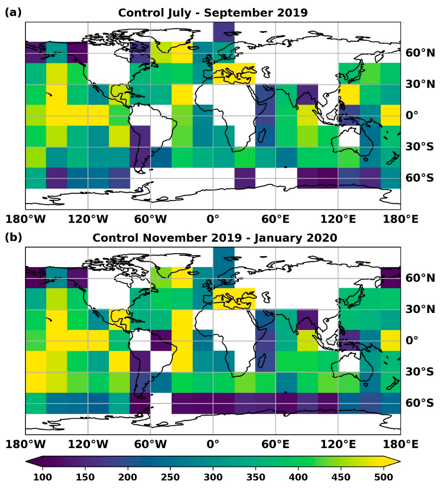
The changes to the O-A statistics for an experimental configuration relative to the control were also calculated and are presented in 20° × 20° boxes. The aim was to visualise the impact of an experimental configuration and to highlight the regions with the most/least impact. To achieve this, the absolute change in the O-A mean differences (Dabs, Equation (1)) and the change ratio of O-A standard deviation (CRS.T.D., Equation (2)) between an experimental configuration and the control OSTIA were calculated using Equations (2) and (3). The mean differences and standard deviation between Argo and OSTIA were also calculated. The numbers of O-A matchups available in each of the 20° × 20° boxes during JAS and JFM are shown in Figure 2. In most boxes, the number of matchups within each 3-month period is over 100. In coastal regions and the Southern Ocean, however, the numbers of matchups are much lower. Negative values indicate improvements in the experimental configurations compared to the control, whilst positive values indicate degradations.
D a b s = M e a n   D i f f e r e n c e E x p e r i m e n t A r g o M e a n   D i f f e r e n c e C o n t r o l A r g o ,
C R S . D . = 100 × S . D . E x p e r i m e n t A r g o S . D . C o n t r o l A r g o / S . D . C o n t r o l A r g o ,

2.4. OSTIA Configurations

Based on the recommendation from the EUMETSAT (see Section 2.1), only QL 5 dual-view SLSTR SSTs were considered in the study, as this subset of SLSTR SSTs is of highest quality and is most suitable to be used in the reference dataset. The options of using all dual-view data and only night-time dual-view data were examined, as for the night-time observations, the connection to foundation SSTs is more straightforward due to the absence of diurnal warming, and the SSTs are expected to be more accurate due to the availability of an extra channel for the retrieval. In addition, the possibility of using SLSTR SST products in combination with VIIRS L3U SSTs as reference sensors was tested in this study. To test the potential advantage of using dual-view SLSTR in the reference dataset in regions affected by aerosol, the quality control (QC) flags of VIIRS and SLSTR SSTs were adjusted in two experiments at the bias correction stage. The resulting reference at each latitudinal range are as the following: between 25°S and 25°N, only SLSTR SSTs were used in the reference; between 50°S and 25°S or between 25°N and 50°N, both SLSTR and VIIRS SSTs were used in the reference; and north of 50°N or south of 50°S, only VIIRS SSTs were used in the reference. For the other experiments combining SLSTR and VIIRS in the reference dataset, all observations within the matchup radius were used for bias correction, regardless of their source.
The operational OSTIA system prior to December 2020 is used as the control, which assimilates both Sentinel-3A and Sentinel-3B SLSTR SSTs and uses VIIRS as the satellite reference sensor, and a total of eight experimental configurations were tested. The details of these configurations are listed in Table 2. Note, the reference datasets in all runs contain in situ observations from drifting and moored buoys; hence, only the satellite sensors are listed here. The control run assimilates both Sentinel-3A and -3B data but they are not used in the reference dataset.

3. Results

Initially, Section 3.1 examines the bias correction of the SLSTR SSTs in the control OSTIA system suite, in which the SLSTR is not used as a reference. Then, the study focuses on the use of Sentinel-3A and -3B SLSTR SSTs in the OSTIA system as part of the reference dataset. First, the impact of using different skin-to-depth adjustments when the SLSTR is the satellite reference sensor is examined (Section 3.2). Then, two main scenarios are considered: one uses the SLSTR as the only satellite sensor in the reference dataset; and the other investigates various ways to combine the SLSTR with the VIIRS as satellite sensors in the reference sensor (Section 3.3).

3.1. SLSTR Bias Correction in Control OSTIA

Before examining the use of the SLSTR as a reference in the OSTIA system, it is useful to present the SLSTR bias correction in the control configuration. In the OSTIA system, all satellite observations are bias-corrected against a reference dataset, which includes the VIIRS SSTs and in-situ observations in the case of the control configuration. Bias fields are generated for each non-reference sensor by analysing differences between sensor data and the reference dataset [1]. The biases are updated daily and use the bias fields from the previous day (after a relaxation towards zero) as the first guess. The resulting bias estimates are removed from the satellite data prior to the data assimilation step which generates the SST analysis. Note that there is no land–sea mask applied to the bias fields in order to allow for the representation of large-scale biases. The bias fields for the merged Sentinel-3A and -3B SLSTR SSTs against the reference dataset are presented here.
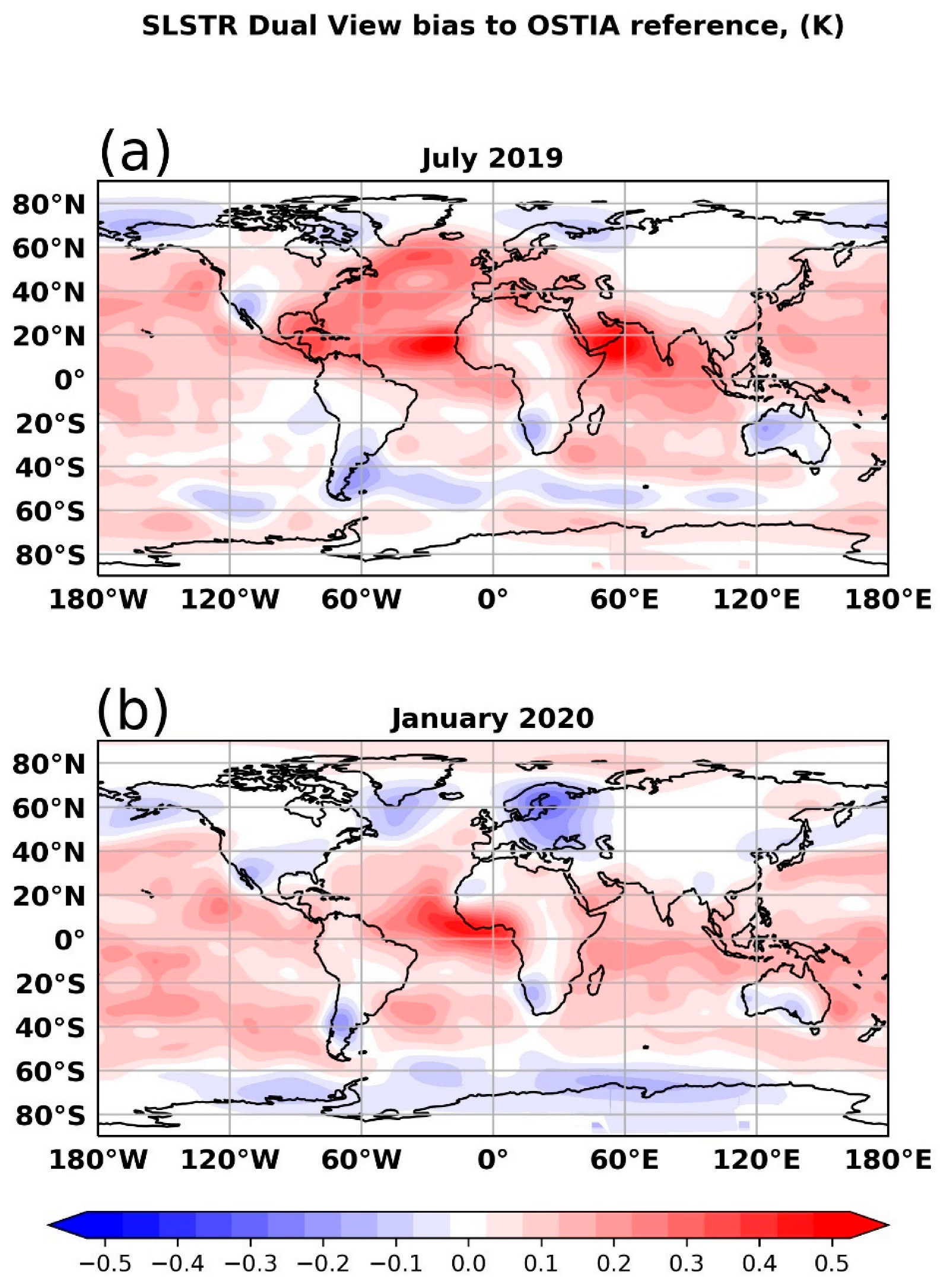
Figure 3 shows the average bias field for the Sentinel-3A and -3B SLSTR dual-view observations against the reference dataset in July 2019 (Figure 3a) and January 2020 (Figure 3b). In both months, the SLSTR dual-view SSTs are warmer than the reference dataset between 40°S and 40°N. The warm biases expand to 60°N in July and to 60°S in January. The largest warm biases can reach 0.6 K in the tropical Atlantic and the Northwest Indian Ocean in July. Small negative biases around 0.1 K are seen in the polar regions north of 60°N and along the Antarctic Circumpolar Current (ACC) region south of 40°S. The reference dataset is largely dominated by the night-time VIIRS SSTs, suggesting the SLSTR dual-view SSTs are warmer than the night-time VIIRS data in most regions. The region for which the most noticeable warm biases occur is the tropical Atlantic, where effects due to the Saharan dust aerosol are observed, especially in JAS, similar to the findings in [18,19]. Stronger plumes of Saharan dust are linked to cooler SSTs in the region of 10–25°N, 20–60°W [20]. With its dual-view capability, the SLSTR could potentially report more accurate SSTs in regions affected by dust aerosols than the VIIRS, although there has not been a dedicated comparison study between the SLSTR and the VIIRS on this matter. Further investigations would be needed to draw a more definite conclusion. The bias field also shows patterns that indicate influence from water vapour, such as the latitudinal distribution in the Atlantic in July and the higher warm bias in the Indian Ocean around the ITCZ (The Intertropical Convergence Zone) in November. There have been studies that found that the OSTIA system has biases with magnitudes that depend on water vapour, and the SLSTR should be less influenced by the water vapour due to its dual-view capability [21,22].

3.2. Skin-to-Depth Conversion for SLSTR SSTs

The skin-to-depth conversion method used in the OSTIA system configuration could have some impact on the results when using the SLSTR in the reference dataset. Only the SLSTR products are available as skin SSTs; all the other satellite products used in the OSTIA system are subskin SSTs, so skin-to-depth conversions are not applied to those products. In previous preliminary tests, skin SLSTR SSTs were converted to depth SSTs by adding a fixed amount of 0.17 K and by calculating a wind-speed-dependent correction and compared when assimilating Sentinel-3A and -3B SLSTR as non-reference sensors. This comparison indicated that it is irrelevant which skin-to-depth conversion is used when the SLSTR data are being bias-corrected to the VIIRS data. However, when the SLSTR data are not bias-corrected, the skin-to-depth conversion is potentially significant. As discussed in Section 2.2, for the majority of tests in this study, the wind-speed-dependent correction was used as it is more scientifically meaningful and provides a better approximation of the skin-to-depth conversion derived from a diurnal cycle model (Figure 1).
In addition to the tests that use the wind-dependent skin-to-depth conversion, an experiment (S3ntRefCS) was performed that was based on the S3ntRef configuration (which uses 3A and 3B night-time SLSTR as reference data) but using the diurnal cool skin model from the OSTIA system diurnal system for the skin-to-depth conversion. The purpose of the experiment was to investigate the potential benefits of using a diurnal model to conduct skin-to-depth conversions. To better assess the impact introduced only by changing the skin-to-depth conversion, another run based on the S3ntRef configuration but using the Fix017 method for the skin-to-depth conversion (S3ntRefFix) was also performed to provide a benchmark for the comparison.
The skin-to-depth conversion using cool skin values from the diurnal OSTIA system was performed using the following steps:
  • An hourly diurnal dataset was assembled to cover the period of the SLSTR data file plus an overlap of +1 h or −1 h from the satellite data time period;
  • For each point of the SLSTR observations, the cool skin value was interpolated to the location and time of the observation, using the SciPy tri-linear interpolation module [23];
  • However, this module is unable to return valid interpolation values (which are within the −1.0–0.0 K range) if filled values are present in the calculation, e.g., close to the coasts. For these observation points, the SciPy nearest neighbour method was used;
  • In the rare cases (approximately 35 out of 2.7 million points) in which the linear interpolation and nearest neighbour methods both failed to return a sensible value (typically at points near a small island), 0.0 was used for the cool skin value. This only occurs when a single island pixel is surrounded by ocean pixels;
  • These interpolated diurnal cool skin values were then applied to the observation dataset to produce the corrected SSTs.
Table 3 and Table 4 show the O-A statistics for three S3ntRef-based configurations that use different skin-to-depth conversion methods during JAS and NDJ. The simple Fix017 method produces lower mean differences from the Argo data than the other two models. However, theoretically, the cool skin values from a diurnal model should be the best method for converting skin-to-depth SSTs, which could suggest that either the Argo data are a biased estimator of foundation SST or that the SLSTR data are too warm.
The DonlonWS mean differences values are very similar to those from the run that used the diurnal OSTIA skin-to-depth conversions, suggesting that it is a good approximation to the diurnal model outputs. The standard deviations of O-A for Fix017 and DonlonWS are comparable, and both perform better than the diurnal cool skin method. The consistency in the mean O-A between the DonlonWS and diurnal OSTIA methods in combination with the standard deviation of O-A being comparable with the Fix017 method supports the use of the DonlonWS method in the other experiments described in this paper.

3.3. The Impact of Assimilating SLSTR in OSTIA and Using It as a Reference Sensor

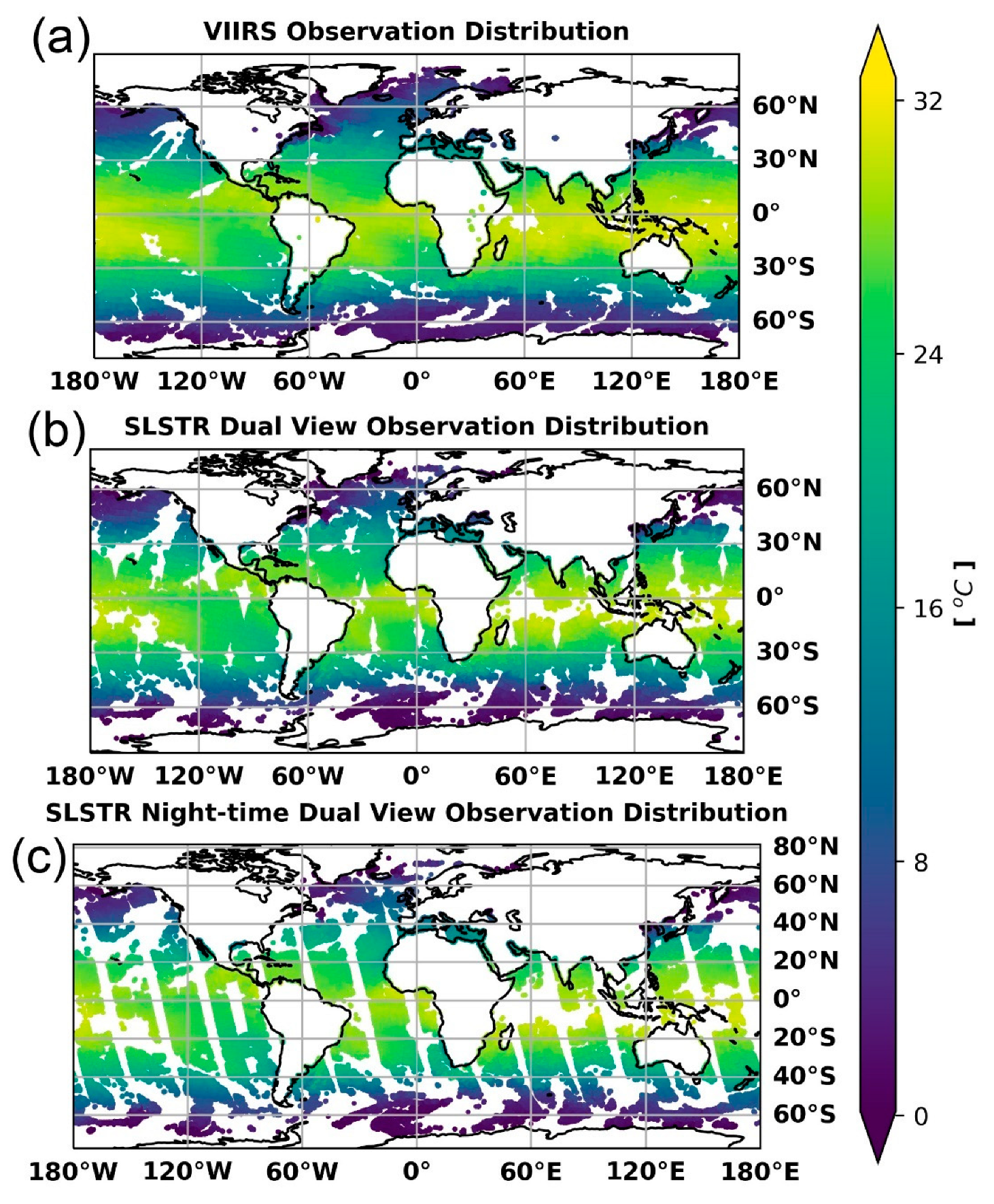
With much improved global data coverage since the launch of the Sentinel-3B satellite, the use of the SLSTR as the satellite reference sensor in the OSTIA system has become more viable. In this section, the impact of using the SLSTR (Sentinel-3A and -3B) in this way is examined. Figure 4 shows the data coverage of the reference dataset in the control, S3Ref and S3ntRef runs on 31 January 2020 as an example. All three datasets provide global coverage, with the VIIRS being the most globally complete and the night-time SLSTR dual-view data having the biggest gaps. The number and coverage of data available as the reference for bias correction influence the analysis quality, and a careful balance needs to be reached to assure the highest-quality subset of SSTs from the reference sensor(s) and enough data to maintain sufficient global coverage.

3.3.1. Replacing VIIRS with SLSTR in the OSTIA Reference Dataset

The impact of replacing the VIIRS SSTs in the reference sensor with the SLSTR SSTs is presented in this section. Two experiments were considered: using all dual-view SLSTR SSTs (S3Ref) and using only night-time dual-view SLSTR SSTs (S3ntRef) in the reference dataset. The results were validated against Argo observations, and O-A statistics were compared to those from the control OSTIA system.
Table 5 and Table 6 show the JAS and NDJ O-A statistics for the experiment and control runs, in which the numbers in bold indicate an improvement in the experimental configurations and the numbers in italics indicate a degradation. For both seasons, the control outputs are colder than Argo observations across all oceanic regions. When using the SLSTR as the reference sensor, the resulting the OSTIA system becomes warmer than the Argo observations for most regions. The S3ntRef analyses are slightly warmer than the S3Ref analysis on average. No significant changes to the O-A standard deviation are observed for S3ntRef or S3Ref in either season in most regions. In the Tropical Atlantic, statistically significant changes are observed in both experiments (0.02 K) in JAS and for the S3ntRef experiment (0.02 K) in NDJ. Improvements of about 0.03 K are also observed in the Indian Ocean for both experiments in JAS. During JAS, a noticeable reduction in the absolute values of the mean differences in the two experiment runs can be seen in some regions including the Tropical Atlantic, Indian Ocean and the Southern Ocean, where the largest reduction reaches 0.11 K. However, a slight degradation in comparison to the control is observed in the North Atlantic and North Pacific and, for S3ntRef, also in the Tropical Pacific. During NDJ, the mean differences are still improved in most regions, except in the Indian Ocean where degradation (an absolute change of 0.02 K in S3Ref and 0.04 in S3ntRef) is observed for both experimental configurations. A degradation of a similar magnitude (0.03 K) is also seen in the Tropical Pacific in the S3ntRef configuration.
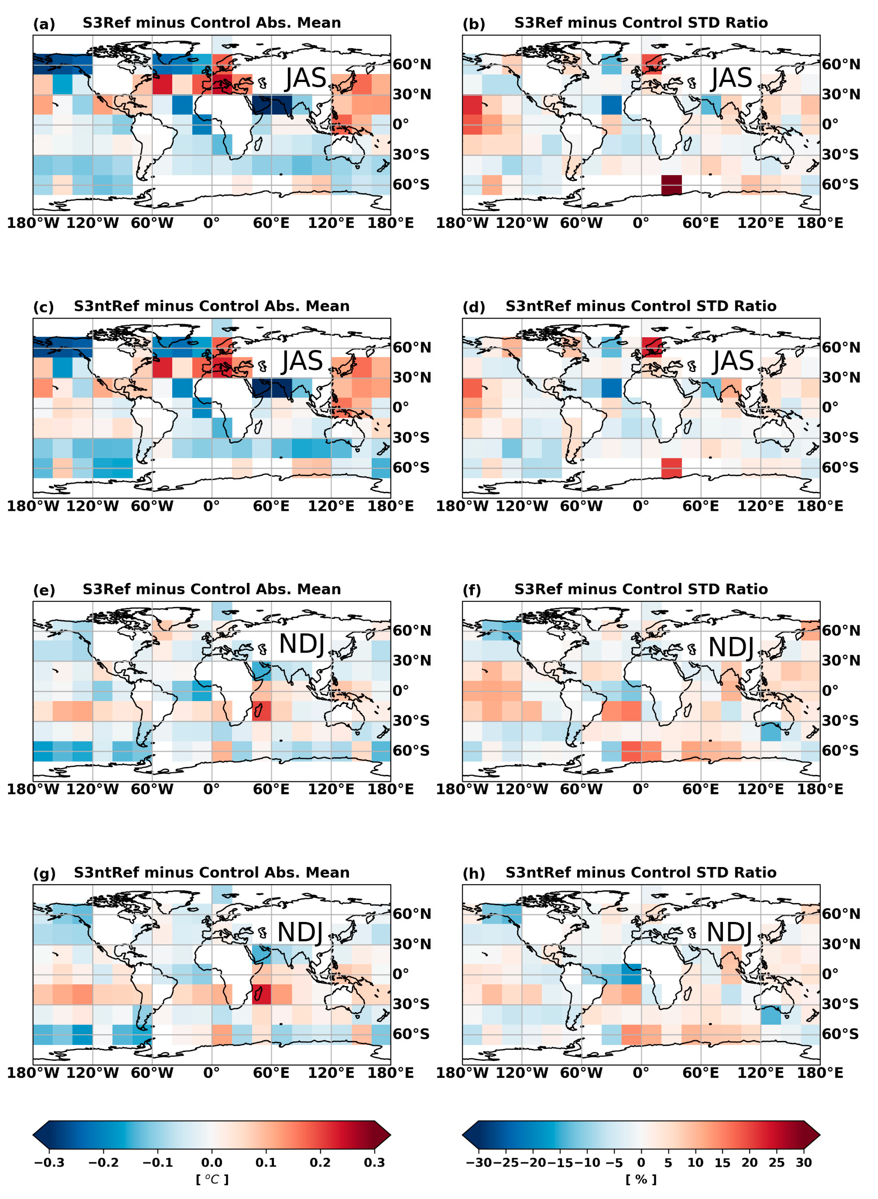
Figure 5 shows the spatial distributions of the absolute changes in the O-A mean difference and the ratio O-A standard deviation changes between the experiments and the control OSTIA system. The spatial patterns of the changes against the control OSTIA system for S3Ref and S3ntRef are similar: improvements in the mean differences and RMS are mainly observed in the Tropical Atlantic, Northeast Pacific, Northwest Indian Ocean and the Southern Ocean in JAS (Figure 5a–d); and improvements are observed in similar regions in NDJ, although the magnitudes are smaller (Figure 5e–h). The O-A statistics in Table 5 for the North Pacific are likely to have been dominated by the degradation in the Western Pacific. There are also differences in the spatial patterns between the S3Ref and S3ntRef configurations: S3Ref performs better in the tropics whilst S3ntRef shows stronger improvements in the Southern Ocean in JAS (see Figure 5a,c). These features are consistent with the averaged statistics in Table 5 and Table 6. The magnitude of improvements or degradations appear to be larger in JAS, and there are greater improvements in JAS than in NDJ, especially in the Indian Ocean.
Overall, replacing the VIIRS with the SLSTR as the reference sensor in the OSTIA system leads to mixed results. Noticeable improvements and degradations are observed. The largest RMS improvement was approximately 30%, and it was about 0.2 K for the mean differences. Considering both seasons, S3Ref presents slightly better results than S3ntRef, especially in the tropical Pacific and Indian Ocean. One consistent feature is that when using the SLSTR in the reference dataset, the OSTIA system becomes warmer than the Argo observations. The increases in the mean difference against Argo for S3Ref or S3ntRef runs reach 0.1 K in some regions compared to those for the control OSTIA system (see Table 5 and Table 6).
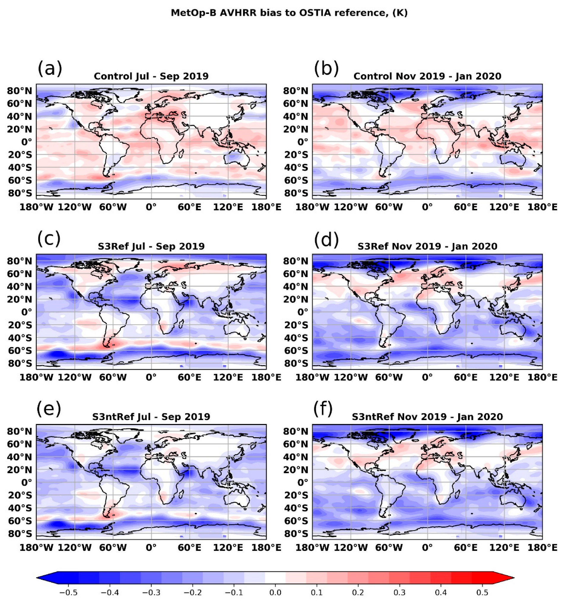
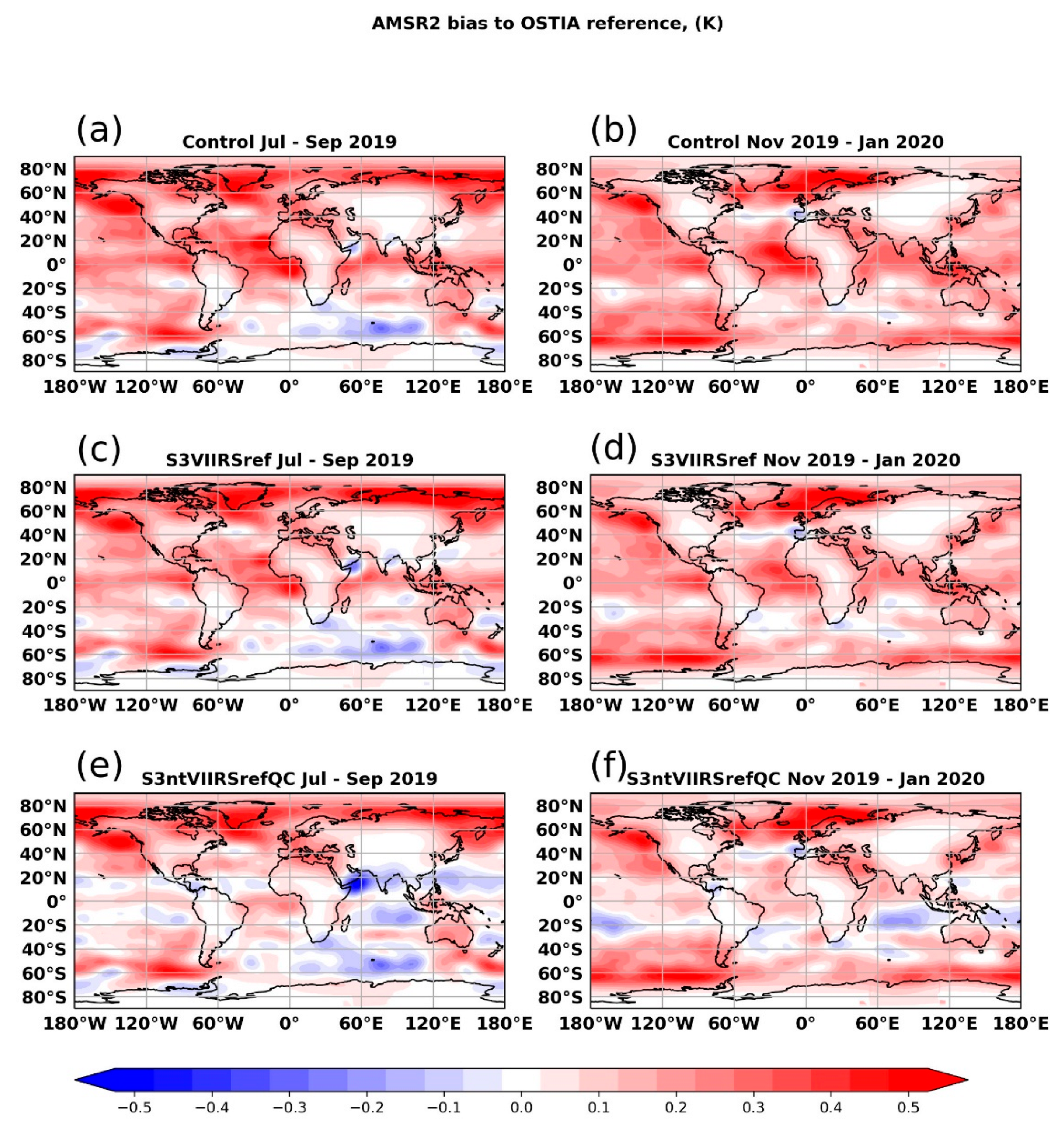
Another way to assess the impact of changing the reference sensor is to examine the bias field for satellite data that are being corrected by the reference dataset. Figure 6 shows the average bias fields for MetOp-B AVHRR in the control run (Figure 6a,b), S3Ref (Figure 6c,d) and S3ntRef (Figure 6e,f) configurations during JAS and NDJ. As the bias fields illustrate the bias to be removed, a warm bias indicates the satellite data are warm compared to the reference, and vice versa.
MetOp-B AVHRR SSTs are generally warmer than the reference dataset in the control run (Figure 6a,b), except in the polar regions, where negative biases are observed. When using the SLSTR as the reference sensor in S3Ref and S3ntRef runs, the bias fields for MetOp-B AVHRR become more negative, suggesting MetOp-B AVHRR observations are colder than the reference datasets in these two configurations. The features are consistent in JAS and NDJ. The bias fields are comparable between the S3Ref and S3ntRef runs. The only regions that show noticeable differences are in the Southern Ocean and the polar area in the northern hemisphere in JAS. In both regions, the slight warm bias in S3Ref either becomes less consistent or disappears in S3ntRef. This indicates that the full set of dual-view SSTs is colder than the night-time-only dual-view SSTs in parts of the high-latitude areas. Similar features are also seen in the Arabian Sea, and these are consistent with the findings of a previous study [24]. The tropical Atlantic region affected by Saharan dust also shows differences between JAS and NDJ, suggesting there is seasonality in the biases [18].
Figure 7 shows the same bias fields but for AMSR2 against the reference datasets. In the control run, AMSR2 is much warmer than the reference during both JAS and NDJ over almost the whole global ocean. When using the SLSTR as the only satellite reference sensor, the AMSR2 bias fields become negative in JAS in the Indian Ocean, Western Pacific and the Southern Ocean. Cold biases also occur during NDJ but mainly in the southern hemisphere, and the magnitude is smaller compared to that during JAS. The S3Ref and S3ntRef runs show very similar spatial patterns (Figure 7c–f).
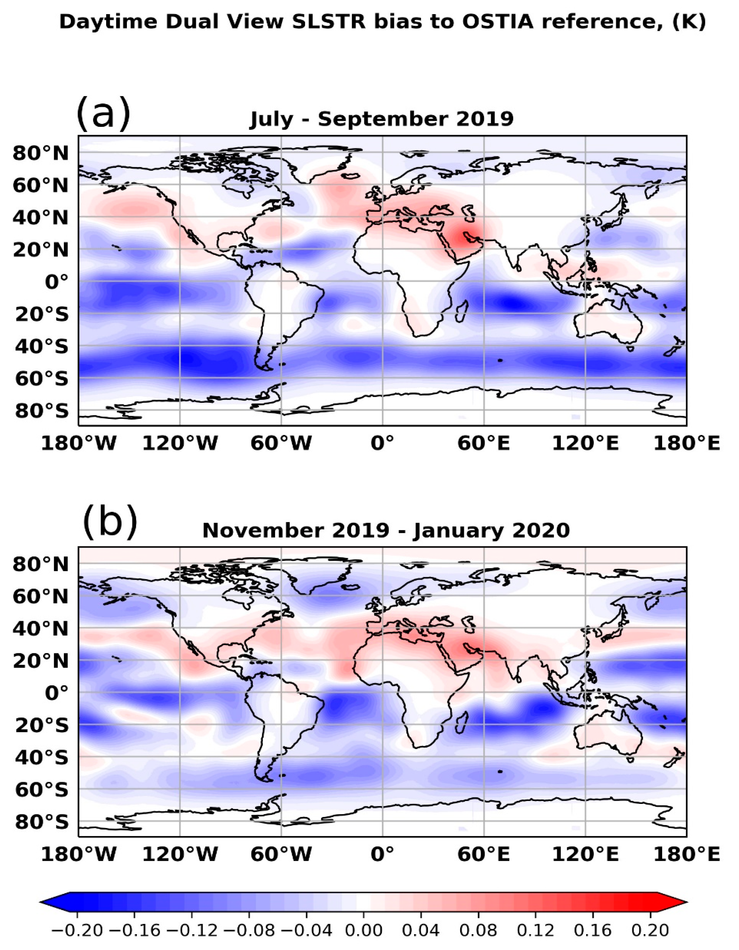
One surprising note regarding S3Ref and S3ntRef is that the analyses become warmer when using the night-time SLSTR as the only satellite reference sensor (see Table 5 and Table 6 for details). Figure 8 shows the average bias field of daytime SLSTR dual-view SSTs against the reference dataset in the S3ntRef run during JAS and NDJ. Although it is not a direct comparison of daytime versus night-time dual-view SLSTRs, the number of in situ observations in the reference dataset is much smaller than the satellite reference, so Figure 8 gives an approximate estimate of how the daytime and night-time SLSTR SSTs compare to one another. The daytime SLSTR SSTs are warmer than the reference north of approximately 20°N in JAS and are slightly cooler in the northern high latitudes and the rest of the global ocean. In NDJ, the daytime SLSTR SSTs are warmer than the references between ~20°N and 40°N across the global ocean and between 20°S and 40°S mainly in the South Pacific. The daytime SSTs appear to be cooler than the reference in other regions. One possible influence on these bias fields is that for the daytime SSTs, any observations with a wind speed below 6 m/s would have been removed prior to the bias correction, which account for slightly less than half of all of the daytime observations, whilst the night-time SSTs from all wind speeds are used, provided they pass the other quality check procedures. Based on Figure 1, it is possible that for SSTs with a wind speed over 6 m/s, Fix0.17 and DonlonWS methods overcorrect these SSTs. DonlonWS also under-correct SSTs with a wind speed under 6 m/s. These could be contributing factors for the slightly warmer night-time SLSTR SSTs than the daytime SSTs, as the night-time SSTs contain SSTs at all wind speeds. However, further investigations would be required to conclusively determine the reasons for these bias fields.

3.3.2. Combining VIIRS and SLSTR in the OSTIA Reference Dataset

A second option for using the SLSTR SSTs in the reference dataset is to combine the data with the VIIRS. As before, the impact of using all dual-view and only night-time dual-view SLSTR SSTs is considered in this section. One advantage of the SLSTR dual-view sensor is its robustness to dust or volcanic aerosols; hence, the SLSTR SSTs are expected to be more accurate in regions impacted by dust or volcanic aerosol. Therefore, the possibility of adjusting the composition of the satellite SSTs in the reference dataset based on where they are expected to be most accurate is also investigated in this section. A straightforward method of implementing this combination was used, in which the reference dataset was split into latitude bands. The procedure to adjust the composition of the reference dataset based on latitude was as follows:
  • Produce reference and satellite (to be bias-corrected) matchups individually for each part of the reference dataset, i.e., so that there are sets of matchups for each of the in situ VIIRS and SLSTR reference components;
  • Adjust the QC values in the matchup files, so that the matchup values against the VIIRS between 25°S and 25°N and the matchup values against the SLSTR south of 50°S and north of 50°N were rejected; no adjustment was made for the matchup values against the in-situ observations;
  • The three matchup files were merged into one to be input into the next bias analysis.
For all four configurations, there are improvements in the O-A mean differences in both periods compared to the control (see Table 7 for JAS statistics and Table 8 for NDJ statistics). The magnitude of the improvements is larger for the two runs with latitudinal adjustments. The S3ntVIIRSrefQC run has the best O-A mean differences in all regions in JAS, except in the Tropical Pacific where the best result is observed for the S3VIIRSrefQC run. The largest improvement (largest reduction in magnitude) in the S3ntVIIRSrefQC run is seen in the Tropical Atlantic, with an improvement of 0.17 K. Improvements of around 0.1 K are also seen in the Indian Ocean (0.13 K), where the impact of dust is expected, and the North Atlantic (0.07 K). In NDJ, the results for S3VIIRSrefQC are also good, with similar reductions in the magnitude of the O-A mean differences as in S3ntVIIRSrefQC, including outperforming it in the Tropical Atlantic and the Tropical Pacific. The magnitude of improvements for the S3VIIRSref and S3ntVIIRSref runs are moderate, with the S3VIIRSref having slightly better overall results. This is possibly because without the latitudinal adjustments, the reference dataset is dominated by the VIIRS, which has more data. The typical ratio of the number of observations for the VIIRS/the SLSTR is 1.6–2.5 for the night-time-only dual-view SLSTR and 1.2–1.8 for the daytime and night-time dual-view SLSTR. Hence, when using both the day and night dual-view SLSTRs in the reference dataset, the number of data from the SLSTRs and the VIIRS reference components are more balanced than in the run that only uses night-time dual-view SLSTR SSTs in the reference dataset without the latitudinal division. Globally, no significant changes occurred for the O-A standard deviation for all four configurations in either season, but there were slight improvements in the Tropical Atlantic in JAS for the S3VIIRSrefQC and S3ntVIIRSrefQC runs.
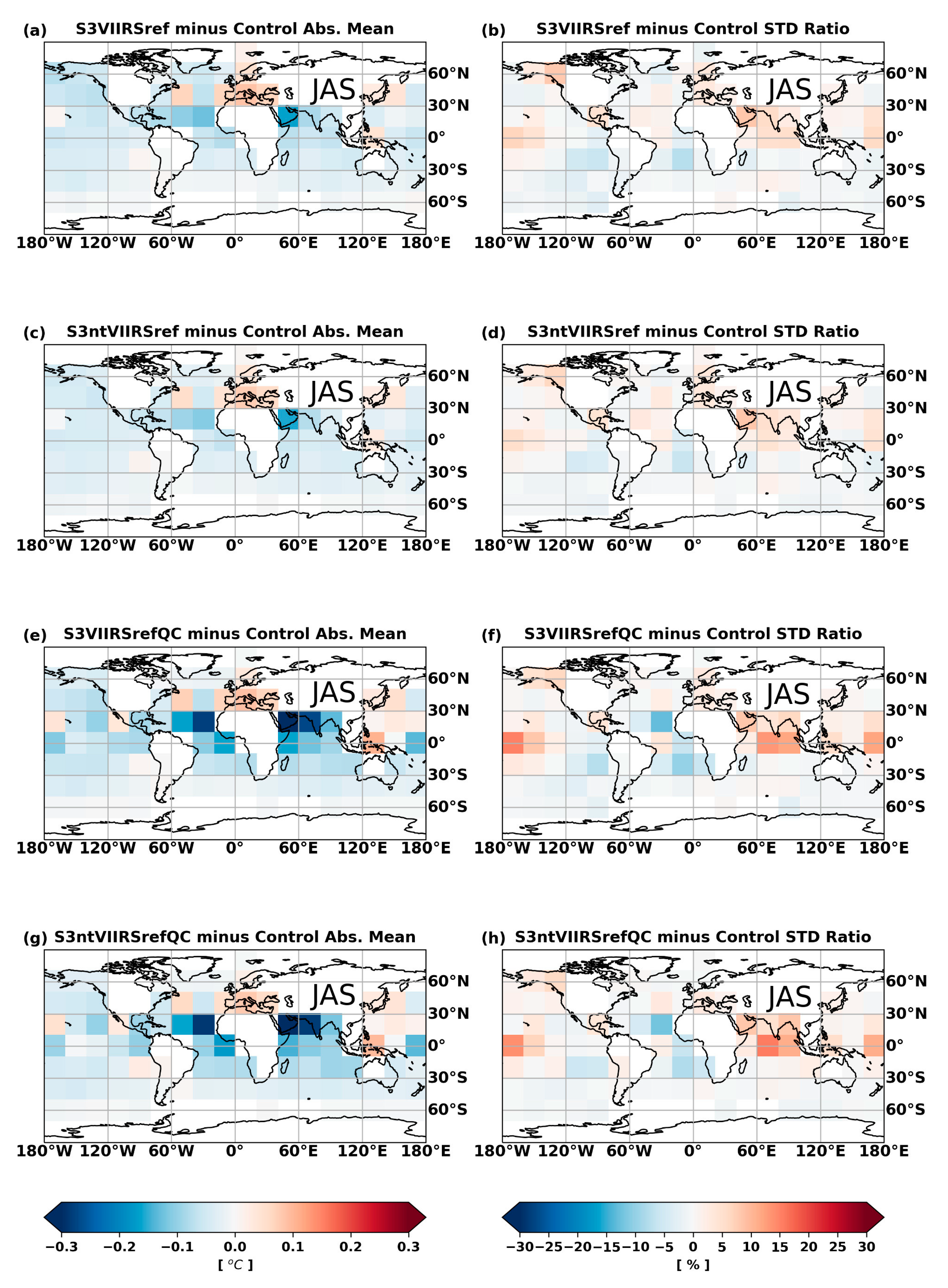
Figure 9 shows the absolute change in the O-A mean difference and the O-A standard deviation change ratio for the four experimental configurations in JAS. S3VIIRSref and S3ntVIIRSref show similar results for both the O-A mean difference and standard deviation change ratio. The largest standard deviation change ratio reaches about 10% in S3VIIRSref and S3ntVIIRSref in the Indian Ocean (Figure 9b,d). In all four runs shown in Figure 9, the O-A mean difference shows degradation in the Mediterranean and the Black Sea. At these latitudes, the reference data contain both VIIRS and SLSTR data, suggesting that by adding the SLSTR data, the resulting analyses were slightly worse than the Argo observations. When using the SLSTR in the reference dataset, the averaged SST in this region increased from 25.67 °C for the control to 25.75 °C for S3VIIRSref (25.74 °C for S3ntVIIRSref), whilst the average of the Argo observations in this region is 25.56 °C. The averaged SSTs for the two runs with latitudinal adjustments are very similar to their corresponding runs without the adjustments. In winter, using the SLSTR in the reference dataset also increased the average SST in this region, but the change is manifested as an improvement due to the analyses being colder than those of the Argo. It is worth noting that although in the Mediterranean, there are 1121 Argo profiles in the summer period, the region is more challenging for Argo floats than open ocean.
With the latitudinal adjustments, the O-A mean differences and standard deviations are further improved in regions where improvements are seen in S3VIIRSref or S3ntVIIRSref. The change patterns are very similar for S3VIIRSrefQC and S3ntVIIRSrefQC (Figure 9e–h). For both runs, the largest improvements in the mean differences are around 0.3 K in the Tropical Atlantic and Northwest Indian Ocean. The largest improvements in standard deviation are seen in the Tropical Atlantic and are between 10% and 15% in both runs. In regions where degradations are observed in S3VIIRSref and S3ntVIIRSref, S3VIIRSrefQC and S3ntVIIRSrefQC show increased degradations. A degradation in the standard deviation up to 15% is observed in the tropical Pacific and Indian Ocean during JAS. This suggests relying on the SLSTR to perform bias correction in the tropical regions improved the mean differences in comparison to the Argo profiles but degraded the standard deviation. One potential explanation is that the averaged conditions in these regions agree better with the Argo when using the SLSTR as the main reference sensor. However, discrepancies between the VIIRS and the SLSTR SSTs and the gaps between swathes could at the same time increase the standard deviation in comparison to that of the Argo.
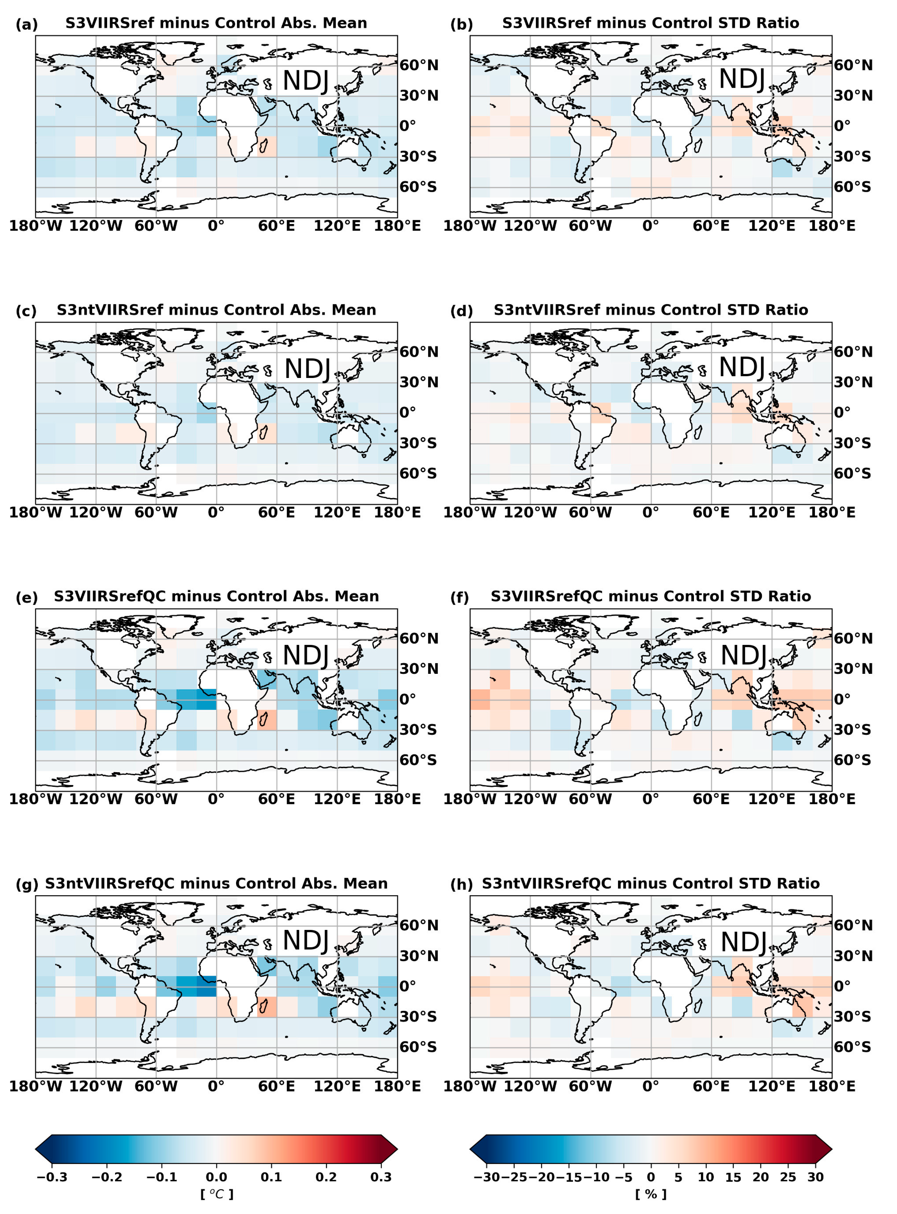
Figure 10 shows the same O-A statistic changes for the four configurations as in Figure 9 but for the NDJ results. The spatial patterns for the runs without latitudinal adjustments are similar to the JAS results, with moderate improvements observed for most of the globe and more noticeable changes in the tropics (Figure 10a–d). The differences between the S3VIIRSref and S3ntVIIRSref runs are smaller than those in JAS. The largest improvement in the mean difference is around 0.1 K and around 5–10% for the standard deviation. With latitudinal adjustments, the configurations show better results, especially in the Tropical Atlantic, where the largest improvements can reach 0.2 K and ~10% for the mean differences and standard deviation, respectively. Regions with over 15% standard deviation changes are smaller in NDJ than in JAS, and a slight degradation is seen in the Tropical Pacific.
Figure 11 presents examples of bias fields from the experimental runs together with the control OSTIA system. The O-A statistics indicate that when combining the SLSTR with the VIIRS SSTs in the reference dataset, there were no significant differences between the runs using both the day and night-time dual-view SLSTR SSTs and the night-time dual-view SLSTR. Therefore, only the bias fields of the S3VIIRSref and S3ntVIIRSrefQC runs are shown. For the S3VIIRSref run, the warm biases in the control OSTIA system for the MetOp-B AVHRR (Figure 11a) are reduced globally but maintain a similar pattern during JAS (Figure 11c), and the cold biases in the southern hemisphere in the control (Figure 11b) propagate further north during NDJ (Figure 11d). For the S3ntVIIRSrefQC run, the most noticeable change is the band of cold bias in the tropics in JAS and the dominance of cold biases in the regions south of 20°N during NDJ. This is consistent with the findings in the previous section that using the SLSTR SSTs in the reference dataset leads to a warmer reference dataset and hence analysis. It is hard to conclude solely from the bias fields whether these changes indicate improvements or degradations for the four experimental configurations compared to the control. However, given that the O-A statistics improve when the experimental configurations are used, it is likely that their bias fields are better representations of the bias in the MetOp-B AVHRR data than those obtained from the control run. This is perhaps expected as the SLSTR dual-view SSTs used within the reference dataset in the experimental configurations are expected to be more robust to the presence of dust aerosol than those from the VIIRS.
Figure 12 shows the bias fields for AMSR2 in S3VIIRSref, S3ntVIIRSrefQC and the control runs. The bias fields for S3VIIRSref are very similar to the fields in the control, suggesting a dominance of the VIIRS SSTs when the observations are bias-corrected. S3ntVIIRSrefQC presents a more different set of bias fields, especially in the tropical region where the bias correction is against the SLSTR SSTs and available in situ observations. Larger areas show cold biases, and the change is more obvious in JAS than in NDJ.

4. Discussion

In this study, the impact of using the SLSTR in the OSTIA system—in particular when using the SLSTR in the reference dataset—has been presented. Multiple ways of using the SLSTR as the reference sensor were investigated, including an experimental method to adjust the composition of the reference dataset based on latitude. Argo reference data were used as the primary way to evaluate the performance of each. These showed that combining the SLSTR with the VIIRS data as the satellite reference sensors is promising, while the runs using the SLSTR as the only satellite sensor in the reference dataset point to areas for further investigation. Three methods for converting the SLSTR skin SSTs to depth SSTs were briefly examined here using the S3ntRef run and two additional runs based on the same configuration (S3ntRefFix, S3ntRef and S3ntRefCS). All three runs that use only the night-time dual-view SLSTR as the reference sensor perform better than the control (see Table 3, Table 4, Table 5 and Table 6 for details) in most regions. Overall, the simple Fix017 (S3ntRefFix run) method produces good results, although the 0.17 K adjustment is too small for SST data when the wind speed is below 6 m/s. Note that the wind speed check in the OSTIA system is only applied to daytime observations, so for night-time SSTs under a low wind speed, the adjusted depth SSTs are potentially cooler than the depth SSTs converted using the other two methods. This discrepancy could be amplified in S3ntRef-based configurations when night-time SLSTR SSTs are the only satellite observations in the reference dataset. Using cool skin values from a diurnal model to convert skin SSTs to depth SSTs is the most sophisticated method of the three. However, it is difficult to estimate the cool skin accurately, and it relies on the accuracy of other parameters in the calculation, such as the NWP wind speed and surface fluxes, which contribute to the results having larger O-A standard deviations than the other two methods. Its implementation in the operational system is also the most complicated and requires the reconfiguration of the OSTIA system. Therefore, while the diurnal cycle model approach is promising, the DonlonWS method currently suits the OSTIA system best, as it approximates the diurnal model and is more practical for operational use.
The results were positive for the use of the SLSTR data in the reference dataset. When combining the two data types without the latitudinal SST QC adjustments, the effective reference dataset is closer to the control run than the two runs with the adjustments, which explains the more moderate changes from the control O-A statistics for the S3VIIRSref and S3ntVIIRSref runs. This is because there are a larger number of the VIIRS SSTs than SLSTRs; therefore, without QC adjustments, the combined VIIRS and SLSTR reference dataset is closer to the VIIRS-only reference dataset than the SLSTR-only reference dataset. It is worth noting that the current latitude scheme for combining the VIIRS and the SLSTR data is a simple method, with only three bands separating the regions potentially influenced by aerosol and clouds. This could be made more sophisticated in a number of ways, such as by using a cloud mask or aerosol products to locate the areas where the SLSTR data could be more accurate. For example, the influence of dust aerosol is significant in the tropical Atlantic, but less so in the tropical Pacific, so the combination of the SLSTR and the VIIRS in the current setup might not be the most suitable for the tropical Pacific. Using the SLSTR data in the reference dataset tends to make the OSTIA system warmer. In many regions, this brings the OSTIA system closer to the Argo system, since the OSTIA system is typically colder than the Argo system. In the Mediterranean, on average, the OSTIA system is warmer than the Argo system in summer when using the SLSTR in the reference dataset and the OSTIA system’s performance against the Argo system is degraded. This is the case whether it is used as the sole sensor or combined with the VIIRS. This indicates that the use of the SLSTR in the OSTIA system reference can be improved further, especially for regional usage. Here, the primary aim was to do an initial test to examine if combining two satellite data in the reference dataset with regional variations is an approach worth pursuing. Therefore, while the latitudinal adjustments are promising, it is currently a very simple scheme, and more investigation would be required before its operational use. There is additionally scope for improving the combination of the reference datasets beyond latitude variations through using statistical methods to homogenise the two datasets.
A further and important consideration when deciding on configuration changes for an operational system is the impact of the change on users. In some cases, the best results from the O-A statistics might not be from the configuration that works best for a particular use case. For example, the OSTIA system was developed to be used as the boundary condition for numerical weather prediction (NWP), and for significant operational OSTIA system changes, NWP trials have traditionally been performed to test the impact. As part of this study, two configurations were tested in Met Office NWP trials and considered for operational implementation: S3ntRef and S3VIIRSref. The results from the NWP trials for the period 15 November 2019–15 January 2020 are shown here. The choice of test period is limited to the NWP setup available at the time of the runs. The NWP results are evaluated by validating the predictions against the Met Office atmospheric analysis and selected observations. The global average and regional standard deviation differences of an NWP trial against each of the analyses or observations are produced. The NWP index is a single value which aims to represent the skill achieved by the model based on the selected statistics [25]. The differences between the NWP index when using an experimental OSTIA system and the NWP index when using the control OSTIA system indicate the impact of the experimental configuration in the NWP system. A positive NWP index change indicates improvements from using the experimental OSTIA compared to the control, and a negative NWP index change indicates degradations from using the experimental OSTIA system. The NWP trials generally need to be a least 6 weeks long to generate robust validation results. It usually takes two weeks for a new OSTIA configuration to spin up in the NWP system; hence, only the period after the spin up is used.
The global NWP index changes for the trials are summarised in Table 9. Normally NWP index changes of around ±0.3 or greater, when combining both oceanic and atmospheric experiments, are considered a significant impact of the experimental configuration. The NWP trial using S3ntRef as the boundary condition performs badly against the analyses compared to the control. However, the S3ntRef trial shows a slight improvement when validated against the observations. The NWP index changes of the S3VIIRSref trial against Met Office analyses and observations are around 0.1, indicating a modest improvement in the S3VIIRSref trial compared to the control.
Degradations in the NWP trials using S3ntRef and S3VIIRSref are mainly seen in the tropical air temperatures at 500 hPa, 800 hPa and 2 m. The exact causes for these degradations need further investigation but it is worth noting that the tropics are the regions where the two OSTIA configurations are more noticeably different to the control OSTIA system, especially for the S3ntRef run. Based on the NWP trial outputs and the results from the O-A statistics, S3VIIRSref was selected for operational implementation in the OSTIA system. The change was implemented in December 2020.
Another feature worth further discussion is the reduction in the O-A mean differences in the tropical Atlantic, Indian Ocean and the Southern Ocean when using the SLSTR dual-view SST as the only satellite reference sensor. Both the S3Ref and S3ntRef runs show sizeable improvements against the Argo data during JAS, with the largest improvement being about 0.11 K. Argo floats are not used in the retrieval of either the VIIRS or the SLSTR SSTs, so they are an independent reference set. This indicates that by referencing the SLSTR, the OSTIA system becomes warmer. As mentioned in previous sections, dual-view sensors are expected to cope with the presence of dust aerosol better than single-view sensors, such as the VIIRS. The biggest reduction in the mean difference for S3Ref and S3ntRef during JAS corresponds to aerosol climatology, which shows a more prominent presence of aerosol in the tropical Atlantic and Indian Ocean during JAS than during NDJ [26]. The presence of aerosol, however, cannot fully explain the mean difference reduction in the Southern Ocean when using the SLSTR as the satellite reference sensor, as the reduction is seen in both JAS and NDJ. Further studies are required to fully understand the impact of changing the satellite reference sensor in the Southern Ocean.

5. Conclusions

This study investigated various ways to use Sentinel-3A and -3B SLSTR SSTs as the reference sensors in the OSTIA system for the bias correction of other satellite data. Only QL 5 dual-view SLSTR SSTs were considered here on advice from EUMETSAT, and the impact of either using the day and night-time dual-view or only the night-time dual-view SLSTR SSTs in the reference dataset was considered. The scenarios investigated were replacing the current reference sensor, the VIIRS, with the SLSTR and combining the VIIRS and the SLSTR as the satellite sensors in the reference dataset.
When using the SLSTR as the only satellite reference sensor, OSTIA-minus-Argo (O-A) statistics indicate a mixed impact when compared to the control O-A statistics, which used the VIIRS as the reference. Sizeable improvements were found in the Tropical Atlantic and Northwest Indian Ocean during JAS for the mean differences. Milder improvements were observed in the global ocean during NDJ without any regions standing out. However, sizeable degradations in the standard deviation were observed in the Pacific in both seasons, with changes in JAS slightly larger than in NDJ. The change in the satellite reference sensor overall leads to a warmer OSTIA system compared to the control. The largest increase in 20° × 20° grid boxes reached 0.3 K based on the O-A statistics. Using the night-time SLSTR SSTs only or combining the daytime and night-time SLSTR SSTs in the reference dataset leads to a 0.02 K difference in the Argo statistics for the global ocean. Note that the O-A mean differences are still negative for the two runs using the SLSTR SSTs in the reference, but the magnitudes are smaller than the control, indicating an improvement against the Argo system.
Combining the VIIRS and SLSTR SSTs in the reference dataset leads to moderate but more consistent improvements in the O-A statistics. The configurations with latitudinal adjustments show the best results, and the differences between using all the SLSTRs or only the night-time dual-view SLSTRs are not significant. The OSTIA system outputs from the four configurations remain largely colder than those of the Argo system, except in a few regions where the O-A mean differences become positive. The S3VIIRSref run was tested in an NWP trial and led to neutral to moderate improvements in the NWP predictions as assessed against analyses and observations. The S3VIIRSref configuration was implemented in December 2020, given its moderate and consistent improvements against the control in the Argo validation statistics and good performance in the NWP trial. In addition, configurations with latitudinal adjustments to balance the SLSTR and VIIRS data suggest that such an approach is promising, although further investigations are required to assure the method is scientifically robust.
The use of the cool skin values from the OSTIA diurnal system to perform the skin-to-depth SST adjustment was also investigated but found to cause an increased O-A standard deviation compared to the control. This requires further investigation.
This study highlights many features that are promising and worth investigations in the future, such as the method used to adjust the composition of the reference dataset based on latitudes. It also highlights areas where the current work could not draw exclusive conclusions but would be useful to fully understand. In particular, a better understanding of the warming impact of the SLSTR in the OSTIA system and its implications would benefit future analyses of SLSTR observations in the OSTIA system and other ocean analyses. The advantage of the dual-view capability of the SLSTR over the VIIRS in regions influenced by dust aerosols should also be investigated further and could lead to the better use of both the SLSTR and VIIRS SSTs. In summary, this study confirms the positive impact the SLSTR has in the OSTIA system but also highlights the need to fully understand the data further to use them effectively in ocean analyses.

Author Contributions

Conceptualization, C.M. and S.G.; methodology, C.M. and S.G.; software, C.M. and M.W.; formal analysis, C.M.; writing—original draft preparation, C.M. and M.W.; writing—review and editing, C.M., S.G. and M.W.; visualisation, C.M. All authors have read and agreed to the published version of the manuscript.

Funding

This work was funded by the UK’s Public Weather Service and the Copernicus Marine Environment Monitoring Service (CMEMS; 78-CMEMS-TAC-SST).

Data Availability Statement

The raw data supporting the conclusions of this article will be made available by the authors on request. HadIOD SIRDS data are available from the Met Office and are © British Crown Copyright, Met Office, 2022, provided under an Open Government License, http://www.nationalarchives.gov.uk/doc/open-government-licence/version/3/ (accessed on 10 September 2024).

Acknowledgments

The authors would like to thank J. Roberts-Jones for providing software that was adapted to visualise the changes in the OSTIA-minus-Argo statistics and for participating in discussions that helped the formation of the methodology of this study. The authors would like to thank C. Tsamalis for discussing the use of the SLSTR in the OSTIA system, presenting the OSTIA system results at the SLSTR Quality Working Group and reviewing early versions of the manuscript.

Conflicts of Interest

The authors declare no conflicts of interest.

References

  1. Good, S.; Fiedler, E.; Mao, C.; Martin, M.J.; Maycock, A.; Reid, R.; Roberts-Jones, J.; Searle, T.; Waters, J.; While, J.; et al. The current configuration of the OSTIA system for operational production of foundation sea surface temperature and ice concentration analyses. Remote Sens. 2020, 12, 720. [Google Scholar] [CrossRef]
  2. Fiedler, E.K.; Mao, C.; Good, S.A.; Waters, J.; Martin, M.J. Improvements to feature resolution in the OSTIA sea surface temperature analysis using the NEMOVAR assimilation scheme. Q. J. R. Meteorol. Soc. 2019, 145, 3609–3625. [Google Scholar] [CrossRef]
  3. While, J.; Mao, C.; Martin, M.J.; Roberts-Jones, J.; Sykes, P.A.; Good, S.A.; McLaren, A.J. An operational analysis system for the global diurnal cycle of sea surface temperature: Implementation and validation. Q. J. R. Meteorol. Soc. 2017, 143, 1787–1803. [Google Scholar] [CrossRef]
  4. Donlon, C.J.; Martin, M.; Stark, J.; Roberts-Jones, J.; Fiedler, E.; Wimmer, W. The Operational Sea Surface Temperature and Sea Ice Analysis (OSTIA) system. Remote Sens. Environ. 2012, 116, 140–158. [Google Scholar] [CrossRef]
  5. Stark, J.D.; Donlon, C.; O’carroll, A.; Corlett, G. Determination of AATSR biases using the OSTIA SST analysis system and a matchup database. J. Atmos. Ocean. Technol. 2008, 25, 1208–1217. [Google Scholar] [CrossRef]
  6. Nardelli, B.B.; Pisano, A.; Tronconi, C. Mediterranean Sea and Black Sea Surface Temperature NRT Data; Copernicus Marine Environment Monitoring Service: Luxembourg, 2019. [Google Scholar]
  7. Donlon, C.; Berruti, B.; Buongiorno, A.; Ferreira, M.-H.; Féménias, P.; Frerick, J.; Goryl, P.; Klein, U.; Laur, H.; Mavrocordatos, C.; et al. The Global Monitoring for Environment and Security (GMES) Sentinel-3 mission. Remote Sens. Environ. 2012, 120, 37–57. [Google Scholar] [CrossRef]
  8. Bonekamp, H.; Montagner, F.; Santacesaria, V.; Loddo, C.N.; Wannop, S.; Tomazic, I.; O’Carroll, A.; Kwiatkowska, E.; Scharroo, R.; Wilson, H. Core operational Sentinel-3 marine data product services as part of the Copernicus Space Component. Ocean Sci. 2016, 12, 787–795. [Google Scholar] [CrossRef]
  9. Merchant, C.J. (SLSTR) Algorithm Theoretical Basis Document. SLSTR-ATBD-L2SST-v2.5, October 2012; pp. 1–54. Available online: https://sentiwiki.copernicus.eu/__attachments/1672112/SLSTR-ATBD-L2SST%20-%20Sentinel%203%20SLSTR%20Level%202%20Sea%20Surface%20Temperature%20ATBD%202012%20-%202.5.pdf?inst-v=c33646ba-3abf-49fb-a1eb-ee14eb9351c0 (accessed on 9 September 2024).
  10. GHRSST Science Team. The Recommended GHRSST Data Specification (GDS) 2.1, Version 0. 2022. Available online: https://zenodo.org/records/6984989 (accessed on 9 September 2024).
  11. Zhang, H.; Beggs, H.; Ignatov, A.; Babanin, A.V. Nighttime cool skin effect observed from infrared SST autonomous radiometer (ISAR) and depth temperatures. J. Atmos. Ocean. Technol. 2020, 37, 33–46. [Google Scholar] [CrossRef]
  12. Donlon, C.J.; Minnett, P.J.; Gentemann, C.; Nightingale, T.J.; Barton, I.J.; Ward, B.; Murray, M.J. Toward improved validation of satellite sea surface skin temperature measurements for climate research. J. Clim. 2002, 15, 353–369. [Google Scholar] [CrossRef]
  13. Artale, V.; Iudicone, D.; Santoleri, R.; Rupolo, V.; Marullo, S.; D’Ortenzio, F. Role of surface fluxes in ocean general circulation models using satellite sea surface temperature: Validation of and sensitivity to the forcing frequency of the Mediterranean thermohaline circulation. J. Geophys. Res. Oceans 2002, 107, 29-1–29-24. [Google Scholar] [CrossRef]
  14. Atkinson, C.; Rayner, N.; Kennedy, J.; Good, S. An integrated database of ocean temperature and salinity observations. J. Geophys. Res. Ocean. Obs. 2014, 119, 7139–7163. [Google Scholar] [CrossRef]
  15. Atkinson, C.; Corlett, G.; Merchant, C. Project: SST-CCI-Phase-II Title: SIRDS Reference Data. 2017. Available online: https://climate.esa.int/media/documents/SST_CCI-SIRDS-UoL-001-Issue1-signed.pdf (accessed on 9 September 2024).
  16. Fiedler, E.K.; McLaren, A.; Banzon, V.; Brasnett, B.; Ishizaki, S.; Kennedy, J.; Rayner, N.; Roberts-Jones, J.; Corlett, G.; Merchant, C.J.; et al. Intercomparison of long-term sea surface temperature analyses using the GHRSST Multi-Product Ensemble (GMPE) system. Remote Sens. Environ. 2019, 222, 18–33. [Google Scholar] [CrossRef]
  17. Fiedler, E.K.; Mao, C.; McLaren, A. SST: Results and Recommendations. Euro-Argo Improvements for the GMES Marine Service (E-AIMS); Report number: D4.3.3; European Commission: Luxembourg, 2015. [Google Scholar]
  18. Tsamalis, C.; Chédin, A.; Pelon, J.; Capelle, V. The seasonal vertical distribution of the Saharan Air Layer and its modulation by the wind. Atmos. Meas. Tech. 2013, 13, 11235–11257. [Google Scholar] [CrossRef]
  19. Capelle, V.; Chédin, A.; Siméon, M.; Tsamalis, C.; Pierangelo, C.; Pondrom, M.; Crevoisier, C.; Crepeau, L.; Scott, N.A. Evaluation of IASI-derived dust aerosol characteristics over the tropical belt. Atmos. Meas. Tech. 2014, 14, 9343–9362. [Google Scholar] [CrossRef]
  20. Foltz, G.R.; McPhaden, M.J. Impact of Saharan Dust on Tropical North Atlantic SST*. J. Clim. 2008, 21, 5048–5060. [Google Scholar] [CrossRef]
  21. Tsamalis, C.; Saunders, R. Quality Assessment of Sea Surface Temperature from ATSRs of the Climate Change Initiative (Phase 1). Remote Sens. 2018, 10, 497. [Google Scholar] [CrossRef]
  22. Merchant, C.J.; Embury, O.; Roberts-Jones, J.; Fiedler, E.; Bulgin, C.E.; Corlett, G.K.; Good, S.; McLaren, A.; Rayner, N.; Morak-Bozzo, S.; et al. Sea surface temperature datasets for climate applications from Phase 1 of the European Space Agency Climate Change Initiative (SST CCI). Geosci. Data J. 2014, 1, 179–191. [Google Scholar] [CrossRef]
  23. SciPy. scipy.interpolate.RegularGridInterpolator. Available online: https://docs.scipy.org/doc/scipy/reference/generated/scipy.interpolate.RegularGridInterpolator.html (accessed on 9 September 2024).
  24. Peyridieu, S.; Chédin, A.; Capelle, V.; Tsamalis, C.; Pierangelo, C.; Armante, R.; Crevoisier, C.; Crépeau, L.; Siméon, M.; Ducos, F.; et al. Characterisation of dust aerosols in the infrared from IASI and comparison with PARASOL, MODIS, MISR, CALIOP, and AERONET observations. Atmos. Meas. Tech. 2013, 13, 6065–6082. [Google Scholar] [CrossRef]
  25. Carroll, E.B.; Hewson, T.D. NWP Grid Editing at the Met Office. Weather. Forecast. 2005, 20, 1021–1033. [Google Scholar] [CrossRef]
  26. Bozzo, A.; Benedetti, A.; Flemming, J.; Kipling, Z.; Rémy, S. An aerosol climatology for global models based on the tropospheric aerosol scheme in the Integrated Forecasting System of ECMWF. Geosci. Model Dev. 2020, 13, 1007–1034. [Google Scholar] [CrossRef]
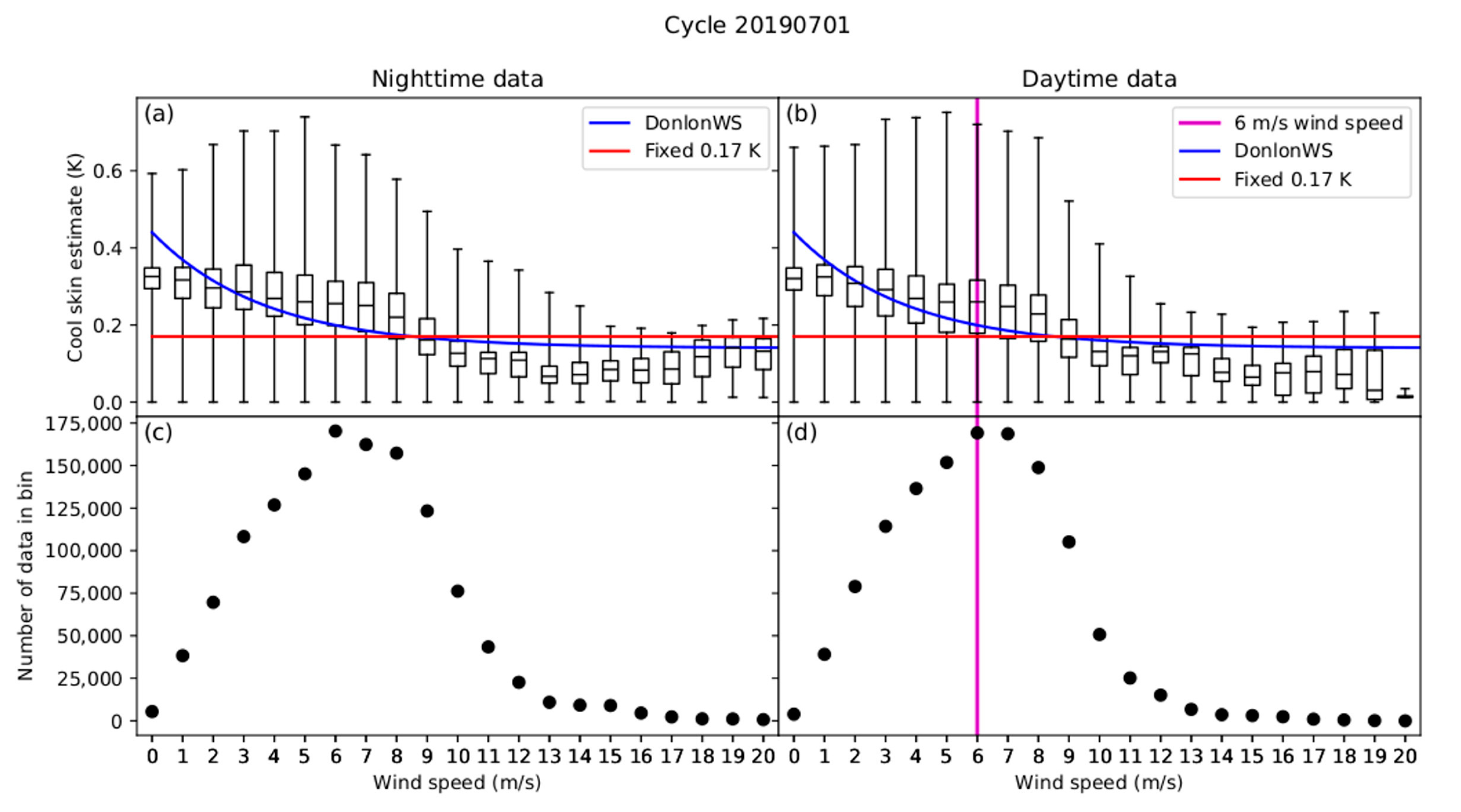
Figure 1. An example of the relationship between wind speed, skin-to-depth conversion values and the number of SST data: (a) skin-to-depth conversions using constant Fix0.17 (red line), DonlonWS (blue line) and diurnal model (boxes with whiskers, with the central line showing the median, the boxes representing the higher and lower quartiles, and the whiskers indicating the maximum and minimum values) against wind speed during night-time; (b) same as (a) but for daytime data; (c) the number of SST data against wind speed during night-time; and (d) same as (c) but for daytime. The vertical cyan line in panel (d) indicates the 6 m/s threshold, below which daytime SST data are rejected.
Remotesensing 16 03396 g001
Figure 2. The number of Argo profiles in each of the 20° × 20° boxes during (a) July–September 2019 and (b) November 2019–January 2020.
Remotesensing 16 03396 g002
Figure 3. Average bias field for merged Sentinel-3A and -3B SLSTR dual-view observations against the reference dataset in: (a) July 2019 and (b) January 2020. Note, there is no land–sea mask applied to the bias fields in order to allow for the representation of large-scale biases.
Remotesensing 16 03396 g003
Figure 4. The coverage of the satellite reference data in the OSTIA configurations on an example day (31 January 2021): (a) Control, (b) S3Ref and (c) S3ntRef. The corresponding satellite SSTs in the three configurations are QL 5 night-time VIIRS SSTs, daytime and night-time dual-view SLSTR SSTs, and night-time dual-view SLSTR SSTs.
Remotesensing 16 03396 g004
Figure 5. The absolute change in OSTIA-minus-Argo mean differences and standard deviation change ratio of OSTIA-minus-Argo for experimental configurations against the control: (a) the change in absolute O-A mean difference for S3Ref during July–September 2019; (b) the standard deviation change ratio of O-A for S3Ref during July–September 2019; (c) the change in absolute O-A mean differences for S3ntRef during July–September 2019; (d) the standard deviation change ratio of O-A for S3ntRef during July–September2019; (e) the change in absolute O-A mean difference for S3Ref during November 2019–January 2020; (f) the standard deviation change ratio of O-A for S3Ref during November 2019–January 2020; (g) the change in absolute O-A mean difference for S3ntRef during November 2019–January 2020; and (h) the standard deviation change ratio of O-A for S3ntRef in during November 2019–January 2020. Blue indicates improvement in the experimental configurations against the control and red indicates degradation against the control.
Remotesensing 16 03396 g005
Figure 6. The averaged bias fields for MetOp-B AVHRR observations in (a) control run over July–September; (b) control run over November–January; (c) S3Ref run over July–September; (d) S3Ref run over November–January; (e) S3ntRef run over July–September; and (f) S3ntRef run over November–January.
Remotesensing 16 03396 g006
Figure 7. The averaged bias fields for AMSR2 observations in (a) control run over July–September; (b) control run over November 2019–January 2020; (c) S3Ref run over July–September 2019; (d) S3Ref run over November 2019–January 2020; (e) S3ntRef run over July–September 2019; and (f) S3ntRef run over November 2019–January 2020.
Remotesensing 16 03396 g007
Figure 8. The bias field of daytime SLSTR dual-view data against the reference field for S3ntRef run for the periods of (a) July–September 2019 and (b) November 2019–January 2020.
Remotesensing 16 03396 g008
Figure 9. The absolute change in OSTIA-minus-Argo mean differences and change ratio of OSTIA-minus-Argo standard deviation for experimental configurations against the control in July–September 2019: (a) the change in absolute O-A mean difference for S3VIIRSref; (b) the change ratio of O-A standard deviation for S3VIIRSref; (c) the change of absolute O-A mean differences for S3ntVIIRSref; (d) the change ratio of O-A standard deviation for S3ntVIIRSref; (e) the change in absolute O-A mean difference for S3VIIRSrefQC; (f) the change ratio of O-A standard deviation for S3VIIRSrefQC; (g) the change in absolute O-A mean difference for S3ntVIIRSrefQC; and (h) the change ratio of O-A standard deviation for S3ntVIIRSrefQC. Blue indicates improvement in the experimental configurations against the control and red indicates degradation against the control.
Remotesensing 16 03396 g009
Figure 10. The change in absolute OSTIA-minus-Argo mean differences and change ratio of OSTIA-minus-Argo standard deviation for experimental configurations against the control in November 2019–January 2020: (a) the change in absolute O-A mean difference for S3VIIRSref; (b) the change ratio of O-A standard deviation for S3VIIRSref; (c) the change in absolute O-A mean differences for S3ntVIIRSref; (d) the change ratio of O-A standard deviation for S3ntVIIRSref; (e) the change in absolute O-A mean difference for S3VIIRSrefQC; (f) the change ratio of O-A standard deviation for S3VIIRSrefQC; (g) the change in absolute O-A mean difference for S3ntVIIRSrefQC; and (h) the change ratio of O-A standard deviation for S3ntVIIRSrefQC. Blue indicates improvement in the experimental configurations against the control and red indicates degradation against the control.
Remotesensing 16 03396 g010
Figure 11. The averaged bias fields for MetOp-B AVHRR observations in (a) control run over July–September 2019; (b) control run over November 2019–January 2020; (c) S3VIIRSref run over July–September 2019; (d) S3VIIRSrun run over November 2019–January 2020; (e) S3ntVIIRSrefQCrun over July–September 2019; and (f) S3ntVIIRSrefQC run over November 2019–January 2020.
Remotesensing 16 03396 g011
Figure 12. The averaged bias fields for AMSR2 observations in: (a) control run over July–September 2019; (b) control run over November 2019–January 2020; (c) S3VIIRSref run over July–September 2019; (d) S3VIIRSrun run over November 2019–January 2020; (e) S3ntVIIRSrefQCrun over July–September 2019; and (f) S3ntVIIRSrefQC run over November 2019–January 2020.
Remotesensing 16 03396 g012
Table 1. Satellite data assimilated in the OSTIA system in December 2019.
InstrumentSatellite MissionOrbit TypeObserving Waveband
AVHRRMetOp-BPolarInfrared
VIIRSS-NPPPolarInfrared
VIIRSNOAA-20PolarInfrared
SLSTRSentinel-3APolarInfrared
SLSTRSentinel-3BPolarInfrared
AMRS2 RSSGCOM-WPolarMicrowave
SEVIRIMeteoSat-11GeostationaryInfrared
Table 2. Details of the control and experimental OSTIA configurations.
OSTIA ConfigurationShort NameSatellite Reference Sensor(s)Skin-to-Depth Conversion
Control OSTIA configuration (representing the operational configuration prior to December 2020)ControlNight-time S-NPP and NOAA-20 VIIRSFixed 0.17 K
Combination of SLSTR and VIIRS in the reference datasetS3VIIRSrefNight-time S-NPP and NOAA-20 VIIRS
plus
Day and night-time dual-view Sentinel-3A and -3B SLSTR
DonlonWS
S3ntVIIRSrefNight-time QL5 S-NPP and NOAA-20 VIIRS
plus
Night-time dual-view Sentinel-3A and -3B SLSTR
Combination of SLSTR and VIIRS in the reference dataset, with latitudinal adjustmentS3VIIRSrefQCNight-time QL5 S-NPP and NOAA-20 VIIRS
plus
Day and night-time dual-view Sentinel-3A and -3B SLSTR
S3ntVIIRSrefQCNight-time QL5 S-NPP and NOAA-20 VIIRS
plus
Night-time dual-view Sentinel-3A and -3B SLSTR
SLSTR replaces VIIRS in the reference datasetS3RefDay and night-time dual-view Sentinel-3A and -3B SLSTR
S3ntRefNight-time dual-view Sentinel-3A and -3B SLSTR
S3ntRefCSApply cool skin from the diurnal OSTIA system
S3ntRef017Fixed 0.17 K
Table 3. OSTIA-minus-Argo statistics for OSTIA S3ntRef-based configurations that use different skin-to-depth conversion methods during 1 July–30 September 2019. Italic font indicates degradation.
RegionMean DifferenceStandard DeviationNum. of Obs.
S3ntRefFixS3ntRefS3ntRefCSS3ntRefFixS3ntRefS3ntRefCS
Global Ocean0.060.090.080.370.380.3933,227
North Atlantic0.120.160.150.500.510.516853
Tropical Atlantic0.060.090.100.240.250.252397
South Atlantic0.000.010.010.420.420.433329
North Pacific0.080.120.110.350.350.378503
Tropical Pacific0.080.110.140.200.200.207307
South Pacific0.030.040.040.250.250.289785
Indian Ocean0.070.090.100.260.260.274199
Southern Ocean0.000.01−0.050.400.400.417030
Table 4. OSTIA-minus-Argo statistics for OSTIA S3ntRef-based configurations that use different skin-to-depth conversion methods during 1 November 2019–31 January 2020. Bold font indicates improvements in the experimental configuration and italic font indicates degradation.
RegionMean DifferenceStandard DeviationNum. of Obs.
S3ntRefFixS3ntRefS3ntRefCSS3ntRefFixS3ntRefS3ntRefCS
Global Ocean0.030.060.070.320.320.3335,251
North Atlantic−0.030.000.030.400.400.417151
Tropical Atlantic0.070.100.140.200.200.212665
South Atlantic0.060.090.080.350.360.373873
North Pacific0.000.020.050.290.290.308266
Tropical Pacific0.080.110.150.180.180.197212
South Pacific0.070.100.090.250.260.2810,788
Indian Ocean0.080.120.160.270.270.274147
Southern Ocean0.030.05−0.020.360.360.378372
Table 5. OSTIA-minus-Argo statistics for OSTIA configurations using SLSTR as the reference sensor and control during 1 July–30 September 2019. Bold font indicates improvements in the experimental configuration and italic indicates degradation.
RegionMean DifferenceStandard DeviationNumber of Obs.
ControlS3RefS3ntRefControlS3RefS3ntRef
Global Ocean−0.100.070.090.380.380.3833,227
North Atlantic−0.080.160.160.500.500.516853
Tropical Atlantic−0.170.060.090.270.250.252397
South Atlantic−0.10−0.020.010.420.420.423329
North Pacific−0.080.110.120.350.350.358503
Tropical Pacific−0.080.080.110.200.200.207307
South Pacific−0.100.000.040.260.260.259785
Indian Ocean−0.160.070.090.290.260.264199
Southern Ocean−0.12−0.040.010.410.410.407030
Table 6. OSTIA-minus-Argo statistics for OSTIA configurations using SLSTR as the reference sensor and control during 1 November 2019–31 January 2020. Bold font indicates improvements in the experimental configuration and italic indicates degradation.
RegionMean DifferenceStandard DeviationNumber of Obs.
ControlS3RefS3ntRefControlS3RefS3ntRef
Global Ocean−0.080.040.060.320.320.3235,251
North Atlantic−0.07−0.010.000.400.400.407151
Tropical Atlantic−0.110.070.100.220.210.202665
South Atlantic−0.080.050.090.350.360.363873
North Pacific−0.090.010.020.290.300.298266
Tropical Pacific−0.080.070.110.180.190.187212
South Pacific−0.090.070.100.260.260.2610,788
Indian Ocean−0.080.100.120.270.270.274147
Southern Ocean−0.110.030.050.360.360.368372
Table 7. OSTIA-minus-Argo statistics for the OSTIA system configurations that combine the SLSTR with the VIIRS as reference sensors and the control during 1 July–30 September 2019. Bold font indicates improvements in the experiments, with the best results shown in bold numbers with an underline.
RegionMean DifferenceStandard DeviationNumber of Obs.
ControlS3VIIRSrefS3ntVIIRSrefS3VIIRSrefQCS3ntVIIRSrefQCControlS3VIIRSrefS3ntVIIRSrefS3VIIRSrefQCS3ntVIIRSrefQC
Global Ocean−0.10−0.06−0.06−0.03−0.020.380.380.380.380.3833,227
North Atlantic−0.08−0.02−0.030.010.010.500.500.500.500.506853
Tropical Atlantic−0.17−0.10−0.11−0.020.000.270.260.270.250.252397
South Atlantic−0.10−0.08−0.08−0.06−0.050.420.420.420.420.423329
North Pacific−0.08−0.03−0.040.000.000.350.350.350.360.368503
Tropical Pacific−0.08−0.04−0.040.020.040.200.200.200.200.207307
South Pacific−0.10−0.08−0.08−0.06−0.050.260.260.260.260.269785
Indian Ocean−0.16−0.10−0.11−0.04−0.030.290.280.280.280.284199
Southern Ocean−0.12−0.11−0.10−0.10−0.100.410.400.410.400.417030
Table 8. OSTIA-minus-Argo statistics for the OSTIA system configurations that combine the SLSTR with the VIIRS as reference sensors and the control during 1 November 2019–31 January 2020. Bold font indicates improvements in the experiments, with the best results shown in bold numbers with an underline.
RegionMean DifferenceStandard DeviationNumber of Obs.
ControlS3VIIRSrefS3ntVIIRSrefS3VIIRSrefQCS3ntVIIRSrefQCControlS3VIIRSrefS3ntVIIRSrefS3VIIRSrefQCS3ntVIIRSrefQC
Global Ocean−0.08−0.05−0.06−0.03−0.020.320.320.320.320.3235,251
North Atlantic−0.07−0.05−0.05−0.03−0.030.400.400.400.400.407151
Tropical Atlantic−0.11−0.05−0.060.010.030.220.210.210.210.212665
South Atlantic−0.08−0.04−0.04−0.02−0.010.350.350.350.350.353873
North Pacific−0.09−0.06−0.07−0.04−0.030.290.290.290.290.298266
Tropical Pacific−0.08−0.03−0.040.020.040.180.180.180.190.187212
South Pacific−0.09−0.04−0.05−0.02−0.020.260.260.260.260.2710,788
Indian Ocean−0.08−0.02−0.030.020.020.270.270.270.270.274147
Southern Ocean−0.11−0.08−0.09−0.08−0.080.360.360.360.360.368372
Table 9. Global NWP index change for the NWP trials using S3ntRef and S3VIIRSref OSTIA compared to the control for the period of 13 November 2019–15 January 2020.
OSTIA Config. 1MO 2 AnalysisObs. 3
S3ntRef−0.150.09
S3VIIRSref0.110.12
1 Configuration; 2 Met Office; 3 Observations.
Disclaimer/Publisher’s Note: The statements, opinions and data contained in all publications are solely those of the individual author(s) and contributor(s) and not of MDPI and/or the editor(s). MDPI and/or the editor(s) disclaim responsibility for any injury to people or property resulting from any ideas, methods, instructions or products referred to in the content.