Four-Dimensional Parameter Estimation for Mixed Far-Field and Near-Field Target Localization Using Bistatic MIMO Arrays and Higher-Order Singular Value Decomposition

Abstract

In this paper, we present a novel four-dimensional (4D) parameter estimation method to localize the mixed far-field (FF) and near-field (NF) targets using bistatic MIMO arrays and higher-order singular value decomposition (HOSVD). The estimated four parameters include the angle-of-departure (AOD), angle-of-arrival (AOA), range-of-departure (ROD), and range-of-arrival (ROA). In the method, we store array data in a tensor form to preserve the inherent multidimensional properties of the array data. First, the observation data are arranged into a third-order tensor and its covariance tensor is calculated. Then, the HOSVD of the covariance tensor is performed. From the left singular vector matrices of the corresponding module expansion of the covariance tensor, the subspaces with respect to transmit and receive arrays are obtained, respectively. The AOD and AOA of the mixed FF and NF targets are estimated with signal-subspace, and the ROD and ROA of the NF targets are achieved using noise-subspace. Finally, the estimated four parameters are matched via a pairing method. The Cramér–Rao lower bound (CRLB) of the mixed target parameters is also derived. The numerical simulations demonstrate the superiority of the tensor-based method.

1. Introduction

Target localization with multiple-input and multiple-output (MIMO) arrays is widely applied to radar, sonar and wireless networks [1,2]. The problem of target localization via direction-of-arrival (DOA) estimation has been extensively investigated focusing on the subspace-based algorithms [3,4] and sparsity-based algorithms [5,6,7]. In the fifth-generation (5G) millimeter-wave communications, the DOA estimation has also been studied in recent years [8,9]. However, these methods are mostly aimed at far-field (FF) target localization. In some scenes such as terahertz (THz) communications in the sixth-generation (6G) networks, the wavefront signal is spherical, and the conventional FF signal model and approach with planar wavefront assumption may suffer from severe performance degradation. Thus, the near-field (NF) signal model is considered [10,11]. Unlike the FF signal model, when a target is localized at the Fresnel region of the array aperture, the wavefront is characterized by both angle and range. For NF source localization, many two-dimensional (2D) parameter estimation approaches of angle and range have been widely investigated [12,13,14]. In addition, a four-dimensional (4D) parameter estimation method including transmit angle, receive angle, transmit range and receive range of NF targets in bistatic MIMO radar has also been presented based on cross-covariance matrices in [15], and a 5D parameter estimation algorithm of frequency, angle, range and polarization parameters of near-field sources has been proposed using parallel factor analysis in [16].

In many actual situations, both the NF and FF targets may usually coexist. Therefore, the mixed localization of NF and FF targets/sources has recently drawn much attention, and several algorithms have been proposed for 2D parameter estimation, including the angle of FF/NF sources and the range of NF source. In [17], an efficient second-order statistic (SOS)-based algorithm called OP-MUSIC has been proposed by constructing the FF and NF estimators and separating the FF sources from the NF ones with the oblique projection technique. To increase parameter estimation accuracy, the higher-order cumulant (HOC), combined with subspace algorithms, has been applied to mixed NF and FF source localization [18,19,20,21,22]. However, the HOC-based algorithms require enough samples to calculate the HOC matrix. With fewer snapshots or single-snapshot, some sparsity-based methods [23,24,25] and Discrete Fractional Fourier Transform (DFrFT)-based methods [26,27] have also been presented for mixed-source localization. These methods have improved the effect of parameter estimation to a certain extent. In addition to methodological improvements, researchers have also focused on the innovation in some special arrays to increase array aperture and optimize resources. In [28,29,30,31,32,33], several new arrays have been used for mixed NF and FF source localization, such as symmetric nested array, symmetric sparse arrays and so on. Despite the fact that the above mixed NF and FF source localization methods have improved accuracy, they are only applicable for 2D parameter estimation. In addition, a 3D mixed FF and NF source localization method with cross-array has also been presented to estimate the 2D angle and range by constructing a range-free cumulant-based vector and a sparse model, respectively [34].

However, in the existing FF and NF source localization algorithms mentioned above, the multidimensional data are stored in a matrix or vector form by means of stacking operation. Although multiple parameters can be estimated, they actually ignore the multidimensional inherent structure of data. The utilization of tensors offers a more intuitive approach for storing and manipulating data with multiple dimensions. Ref. [35] offers a comprehensive examination of tensor analysis in the context of wireless communications and MIMO arrays, and includes a discussion on fundamental tensor operations and common tensor decompositions. For FF localization via angle estimation with MIMO array, several tensor-based methods have been proposed [36,37,38,39], which mainly utilize the parallel factor (PARAFAC) decomposition or the Tucker decomposition. For NF localization by angle and range estimation, a PARAFAC decomposition-based method for a bistatic MIMO system has been proposed on a slightly simple signal model whereby the distance from the centers of the transmitter and receiver arrays to the reference point is assumed to be known [40]. Nevertheless, in the above methods, only the 2D parameters (angle and range) are considered.

In this paper, we present a novel four-dimensional (4D) parameter estimation method to localize the mixed FF and NF targets using bistatic MIMO arrays and higher-order singular value decomposition (HOSVD). The estimated four parameters include the angle-of-departure (AOD), angle-of-arrival (AOA), range-of-departure (ROD) and range-of-arrival (ROA). In the proposed method, we store array data in a tensor form to preserve the inherent multidimensional properties of the array data. First, we arrange the observation data into a third-order tensor and calculate their covariance tensor. Then, we perform the higher-order singular value decomposition (HOSVD) of the covariance tensor. From the left singular vector matrices of the corresponding module expansion of the covariance tensor, we can obtain the subspaces with respect to transmit and receive arrays, respectively. Utilizing the two signal-subspaces associated with transmit and receive arrays, we construct two spectrum functions to estimate the AOD and AOA of the mixed FF and NF targets by 1D spectral searches. Then, using the two noise-subspaces concerning the transmit and receive arrays, we build the other two spectrum functions to obtain the ROD and ROA of the NF targets based on the estimates of AOD and AOA and via 1D spectral searches. Finally, all the estimated parameters are matched via a matching algorithm. The Cramér–Rao lower bound (CRLB) of the mixed target parameters is also derived.

Notations: Scalars are represented by italicized letters, column vectors by lowercase bold letters, matrices by uppercase bold letters, and tensors by bold calligraphic letters. The superscripts ${\left(·\right)}^T$, ${\left(·\right)}^{*}$ and ${\left(·\right)}^H$ are referred to as the transpose, conjugate operators and Hermitian transpose, respectively; ⊙, ⊗ and ⋄, respectively, denote the Hadamard–Schur, Kronecker and the Khatri–Rao product (columnwise Kronecker product). The operation diag(·) is used to represent diagonalization, while the functions rank (·) and det(·) refer to the rank operator and the determinant of a matrix, respectively. vec(·) denotes the vectorization operator, tr(·) denotes the trace operator, and Re(·) denotes the real-part operator of a complex number. For the calculation of tensors, ${•}_n$ denotes the n-mode inner product of a tensor, and ${\times }_n$ denotes the n-mode product of a tensor.

2. Preliminaries

In contrast to a matrix, a tensor is regarded as a mathematics tool for depicting a multidimensional array [41]. An N-order tensor can be denoted as $\mathcal{X}\in {\mathbb{C}}^{I_1\times I_2\times \cdots \times I_N}$, where the elements correspond to the higher-dimensional equivalent of rows and columns in matrices. The tensor operations outlined in our study align with those presented in [42] and include the following procedures.

The matricization or unfolding of tensors can be defined as follows. The n expansion of a tensor $\mathcal{X}\in {\mathbb{C}}^{I_1\times I_2\times \cdots \times I_N}$ of order N is represented as ${\left[\mathcal{X}\right]}_{\left(n\right)}$. The $(i_1,i_2,\cdots ,i_N)$-th element of $\mathcal{X}$ corresponds to the $(i_n,j)$-th element of ${\left[\mathcal{X}\right]}_{\left(n\right)}$, where $j=1+{\sum }_{k=1,k\ne n}^N(i_k-1)J_k$ with $J_k={\prod }_{m=1,m\ne n}^{k-1}{I}_m$.

Additionally, the matrix unfolding of tensor $\mathcal{X}$ along its n-th mode is represented as ${\left[\mathcal{X}\right]}_{\left(n\right)}$ and can be interpreted as a matrix that encompasses all the n-mode vectors of tensor $\mathcal{X}$. The arrangement of the columns is determined based on a specified criterion as referenced in [42].

The n-mode inner product between a tensor $\mathcal{X}\in {\mathbb{C}}^{I_1\times I_2\times \cdots \times I_N}$ and a tensor $\mathcal{Y}\in {\mathbb{C}}^{J_1\times J_2\times \cdots \times J_M}$ is formally specified; when $I_n=J_n$, $n\le min\{M,N\}$, it is presented as $\mathcal{Z}=\mathcal{X}{•}_n\mathcal{Y}\in {\mathbb{C}}^{I_1\times I_2\times \cdots \times I_{n-1}\times I_{n+1}\times \dots \times I_N\times J_1\times J_2\times \cdots \times J_{n-1}\times J_{n+1}\times \cdots \times J_M}$, where

$$\begin{array}{c}{z}_{i_1,i_2,\dots ,i_{n-1},i_{n+1},\dots ,i_N,j_1,j_2,\dots ,j_{n-1},j_{n+1},\dots ,j_M}\hfill \\ ={\displaystyle \sum _{i_n=1}^{I_n}}{x}_{i_1,i_2,\dots ,i_N}·y_{j_1,j_2,\dots ,j_{n-1},i_n,j_{n+1},\dots ,j_M}\hfill \end{array}$$

(1)

The n-mode product of a tensor $\mathcal{X}\in {\mathbb{C}}^{I_1\times I_2\times \cdots \times I_N}$ and a matrix $\mathbf{A}\in {\mathbb{C}}^{J_n\times I_n}$ along the n-th mode is represented as $\mathcal{Y}=\mathcal{X}{\times }_n\mathbf{A}\in {\mathbb{C}}^{I_1\times I_2\times \cdots \times I_{n-1}\times J_n\times I_{n+1}\times \cdots \times I_N}$. This operation is computed by

$$y_{i_1,i_2,\cdots ,i_{n-1},j_n,i_{n+1},\cdots ,i_N}=\sum _{i_n=1}^{I_n}{x}_{i_1,i_2,\cdots ,i_N}·a_{j_n,i_n}$$

(2)

This operation can be conceptualized by applying the matrix $\mathbf{A}$ to all n-mode vectors of $\mathcal{X}$ on the left-hand side. The n-mode product demonstrates the following characteristics:

$$\mathcal{Y}=\mathcal{X}{\times }_n\mathbf{A}\iff {\left[\mathcal{Y}\right]}_{\left(n\right)}{=\mathbf{A}[\mathcal{X}]}_{\left(n\right)}$$

(3)

$$\left\{\begin{array}{c}\mathcal{X}{\times }_n\mathbf{A}{\times }_m\mathbf{B}=\mathcal{X}{\times }_m\mathbf{B}{\times }_n\mathbf{A},m\ne n\\ \mathcal{X}{\times }_n\mathbf{A}{\times }_n\mathbf{B}=\mathcal{X}{\times }_n(\mathbf{BA})\end{array}\right.$$

(4)

The Tucker decomposition or higher-order SVD (HOSVD) of a tensor $\mathcal{X}\in {\mathbb{C}}^{I_1\times I_2\times \cdots \times I_N}$ is defined as

$$\mathcal{X}=\mathbf{\varsigma }{\times }_1{\mathbf{A}}_1{\times }_2{\mathbf{A}}_2\times \dots {\mathbf{A}}_N$$

(5)

where $\mathbf{\varsigma }\in {\mathbb{C}}^{J_1\times J_2\times \cdots \times J_N}$ indicates a core tensor that satisfies the all-orthogonality conditions [42] and ${\mathbf{A}}_n\in {\mathbb{C}}^{I_n\times J_n},n=1,2,\cdots N$ are the unitary matrices consisting of singular vectors in the n-mode.

3. Tensor-Based 4D Parameter Estimation for Mixed FF and NF Target Localization

3.1. Signal Model

Consider a bistatic MIMO array with symmetrical uniform linear arrays of $2M+1$ transmit and $2N+1$ receive omnidirectional antennas, where $d_t$ and $d_r$ denote the inter-element spacings at the transmitter and receiver, respectively. Assume that there are $K=K_1+K_2$ noncoherent mixed FF and NF narrowband targets, including $K_1$ targets in the FF and other $K_2$ targets in the NF. For the k-th target, $k=1,\cdots ,K$, its AOD, AOA, ROD and ROA are denoted by ${\theta }_{tk}$, ${\theta }_{rk}$, $r_{tk}$ and $r_{rk}$, respectively. Let the center of array be the phase reference point whose index is zero, as shown in Figure 1.

In a noisy environment, following the process of sampling, recombination and matched filtering using the orthogonal transmit waveform, the observation from the m-th transmit sensor to the n-th sensor in the l-th independent snapshot can be expressed as

$$\begin{array}{cc}\hfill y_{m,n,l}& =\sum _{k=1}^{K_2}{b}_k^{\left(l\right)}{e}^{j(m{\alpha }_{tk}+m^2{\beta }_{tk})}\times e^{j(n{\alpha }_{rk}+n^2{\beta }_{rk})}\hfill \\ \hfill & +\sum _{k=1}^{K_1}{b}_k^{\left(l\right)}{e}^{j\left(m{\alpha }_{tk}\right)}\times e^{j\left(n{\alpha }_{rk}\right)}+z_{m,n,l}\hfill \end{array}$$

(6)

for $m=1,\cdots ,2M+1$; $n=1,\cdots ,2N+1$, and $l=1,2,\cdots ,L$. Here, $b_k^{\left(l\right)}$ denotes the scattering coefficient of the k-th target during the l-th snapshot. $z_{m,n,l}$ represents Gaussian white noise, with mean value zero and variance ${\sigma }_z^2$. When the k-th target is in the NF, the range belongs to the Fresnel region [43], i.e., $r\in \left[0.62{\left(D^3/\lambda \right)}^{1/2}2D^2/\lambda \right]$, where $\lambda$ is the wavelength and D represents the array aperture. As for the FF target, we can observe that it is a special case of the NF target when $r\to \infty$. Therefore, ${\alpha }_{tk}$ and ${\beta }_{tk}$ for the transmit array can be written as

$${\alpha }_{tk}=-2\pi d_{t}sin{\theta }_{tk}/\lambda$$

(7)

$${\beta }_{tk}=\pi d_t^2{cos}^2{\theta }_{tk}/\left(\lambda r_{tk}\right)$$

(8)

and ${\alpha }_{rk}$ and ${\beta }_{rk}$ for the receive array can be given by

$${\alpha }_{rk}=-2\pi d_{r}sin{\theta }_{rk}/\lambda$$

(9)

$${\beta }_{rk}=\pi d_r^2{cos}^2{\theta }_{rk}/\left(\lambda r_{rk}\right)$$

(10)

Traditionally, the observed data $y_{m,n,l}$ are arranged into a vector ${\mathbf{y}}^{\left(l\right)}\in {\mathbb{C}}^{(2M+1)(2N+1)\times 1}$, given by

$${\mathbf{y}}^{\left(l\right)}=\mathbf{A}({\theta }_t,{\theta }_r,r_t,r_r){\mathbf{b}}^{\left(l\right)}+{\mathbf{z}}^{\left(l\right)}$$

(11)

for $l=1,2,\cdots ,L$, where ${\mathbf{b}}^{\left(l\right)}$ denotes the target complex amplitude vector. ${\mathbf{z}}^{\left(l\right)}$ is the noise vector. $\mathbf{A}({\theta }_t,{\theta }_r,r_t,r_r)={\mathbf{A}}_r({\theta }_r,r_r))\diamond {\mathbf{A}}_t({\theta }_t,r_t)$ denotes the joint steering matrix, with ${\mathbf{A}}_t({\theta }_t,r_t)$ and ${\mathbf{A}}_r({\theta }_r,r_r)$ being the transmit and receive steering matrices, respectively, which contain the components of FF and NF targets, i.e.,

$$\mathbf{A}({\theta }_t,{\theta }_r,r_t,r_r)=\left[{\mathbf{A}}_F({\theta }_t,{\theta }_r){\mathbf{A}}_N({\theta }_t,{\theta }_r,r_t,r_r)\right]$$

(12)

where

$$\begin{array}{cc}\hfill {\mathbf{A}}_F({\theta }_t,{\theta }_r)=& {\mathbf{A}}_{Fr}\left({\theta }_r\right)\diamond {\mathbf{A}}_{Ft}\left({\theta }_t\right)\hfill \\ \hfill =& [{\mathbf{a}}_{Fr}\left({\theta }_{r1}\right)\otimes {\mathbf{a}}_{Ft}\left({\theta }_{t1}\right),\cdots ,{\mathbf{a}}_{Fr}\left({\theta }_{r{K}_1}\right)\otimes {\mathbf{a}}_{Ft}\left({\theta }_{t{K}_1}\right)]\hfill \end{array}$$

(13)

$$\begin{array}{cc}\hfill {\mathbf{A}}_N({\theta }_t,{\theta }_r,r_t,r_r)=& {\mathbf{A}}_{Nr}({\theta }_r,r_r)\diamond {\mathbf{A}}_{Nt}({\theta }_t,r_t)\hfill \\ \hfill =& [{\mathbf{a}}_{Nr}\left({\theta }_{r1},r_{r1}\right)\otimes {\mathbf{a}}_{Nt}\left({\theta }_{t1},r_{t1}\right),\cdots ,\hfill \\ \hfill & {\mathbf{a}}_{Nr}\left({\theta }_{r{K}_2},r_{r{K}_2}\right)\otimes {\mathbf{a}}_{Nt}\left({\theta }_{t{K}_2},r_{t{K}_2}\right)]\hfill \end{array}$$

(14)

where

$${\mathbf{a}}_{Ft}\left({\theta }_{tk}\right)={[exp(-jM{\alpha }_{tk}),\cdots ,1,\cdots ,exp\left(jM{\alpha }_{tk}\right)]}^T$$

(15)

$${\mathbf{a}}_{Fr}\left({\theta }_{rk}\right)={[exp(-jN{\alpha }_{rk}),\cdots ,1,\cdots ,exp\left(jN{\alpha }_{rk}\right)]}^T$$

(16)

$$\begin{array}{cc}\hfill {\mathbf{a}}_{Nt}\left({\theta }_{tk},r_{tk}\right)=& [exp(-jM{\alpha }_{tk}+j{(-M)}^2{\beta }_{tk}),\cdots ,\hfill \\ \hfill & 1,\cdots ,exp(jM{\alpha }_{tk}+j{M}^2{\beta }_{tk}){]}^T\hfill \end{array}$$

(17)

$$\begin{array}{cc}\hfill {\mathbf{a}}_{Nr}\left({\theta }_{rk},r_{rk}\right)=& [exp(-jN{\alpha }_{rk}+j{(-N)}^2{\beta }_{rk}),\cdots ,\hfill \\ \hfill & 1,\cdots ,exp(jN{\alpha }_{rk}+j{N}^2{\beta }_{rk}){]}^T\hfill \end{array}$$

(18)

The observed vector ${\mathbf{y}}^{\left(l\right)}$ for $l=1,\cdots ,L$ can be collected to form a matrix $\mathbf{Y}\in {\mathbb{C}}^{(2M+1)(2N+1)\times L}$ as

$$\mathbf{Y}={\mathbf{A}}_r({\theta }_r,r_r)\diamond {\mathbf{A}}_t({\theta }_t,r_t)\mathbf{B}+\mathbf{Z}$$

(19)

where $\mathbf{Y}={\left[{\mathbf{y}}^{\left(1\right)},\cdots ,{\mathbf{y}}^{\left(L\right)}\right]}^T$, $\mathbf{B}={\left[{\mathbf{b}}^{\left(1\right)},\cdots ,{\mathbf{b}}^{\left(L\right)}\right]}^T$ and $\mathbf{Z}={\left[{\mathbf{z}}^{\left(1\right)},\cdots ,{\mathbf{z}}^{\left(L\right)}\right]}^T$ represent the observation matrix, target scattering coefficient matrix and noise matrix, respectively.

From (11) and (19), we see that the observation $y_{m,n,l}$ is traditionally expressed as the form of a vector or a matrix via stacking operation. In this paper, $y_{m,n,l}$ can be directly arranged into a third-order tensor $\mathcal{Y}\in {\mathbb{C}}^{(2M+1)\times (2N+1)\times L}$, i.e.,

$$\mathcal{Y}=\mathbf{\iota }{\times }_1{\mathbf{A}}_t{\times }_2{\mathbf{A}}_r{\times }_3\mathbf{B}+\mathcal{Z}$$

(20)

where $\mathbf{\iota }\in {\mathbb{C}}^{K\times K\times K}$ is an identity tensor and ${\mathbf{A}}_t$ and ${\mathbf{A}}_r$ are the simplified expressions of ${\mathbf{A}}_t({\theta }_t,r_t)$ and ${\mathbf{A}}_r({\theta }_r,r_r)$. Clearly, we have $\mathbf{Y}={\left[\mathcal{Y}\right]}_{\left(3\right)}^T$ and $\mathbf{Z}={\left[\mathcal{Z}\right]}_{\left(3\right)}^T$.

Based on this tensor-based observation model in (20), we aim at estimating the 4D parameters ${\theta }_t,{\theta }_r$, $r_t$ and $r_r$.

3.2. Algorithm

At first, the sample covariance tensor of $\mathcal{Y}$ is calculated. As per the definition pertaining to the multiplication of two tensors, a fourth-order tensor denoted as $\mathcal{R}\in {\mathbb{C}}^{(2M+1)\times (2N+1)\times (2M+1)\times (2N+1)}$ can be obtained as follows:

$$\mathcal{R}={\displaystyle \frac{1}{L}}\mathcal{Y}{•}_3{\mathcal{Y}}^{*}$$

(21)

Then, the HOSVD is introduced as

$$\mathcal{R}=\mathbf{\varsigma }{\times }_1{\mathbf{U}}_1{\times }_2{\mathbf{U}}_2{\times }_3{\mathbf{U}}_3{\times }_4{\mathbf{U}}_4$$

(22)

In the given expression, the symbol $\mathbf{\varsigma }\in {\mathbb{C}}^{(2M+1)\times (2N+1)\times (2M+1)\times (2N+1)}$ represents the core tensor, while the matrices ${\mathbf{U}}_i$ for $i=1,2,3,4$ represent the left singular vectors corresponding to the i-module decomposition of $\mathcal{R}$, which is written as

$${\left[\mathcal{R}\right]}_{\left(i\right)}={\mathbf{U}}_i{\Sigma }_i{\mathbf{V}}_i^H(i=1,2,3,4)$$

(23)

where ${\mathbf{U}}_1={\mathbf{U}}_3^{*}$ and ${\mathbf{U}}_2={\mathbf{U}}_4^{*}$.

Then, to reduce the noise component, we utilize the truncated HOSVD of the tensor $\mathcal{R}$, written as

$${\mathcal{R}}_s={\mathbf{\varsigma }}_s{\times }_1{\mathbf{U}}_{1s}{\times }_2{\mathbf{U}}_{2s}{\times }_3{\mathbf{U}}_{1s}^{*}{\times }_4{\mathbf{U}}_{2s}^{*}$$

(24)

where ${\mathbf{\varsigma }}_s\in {\mathbb{C}}^{K\times K\times K\times K}$ is the core tensor. ${\mathbf{U}}_{1s}\in {\mathbb{C}}^{(2M+1)\times K}$ and ${\mathbf{U}}_{2s}\in {\mathbb{C}}^{(2N+1)\times K}$ refer to the inclusion of the column vectors of ${\mathbf{U}}_1$ and ${\mathbf{U}}_2$ that correspond to the K dominant singular values, respectively. On the basis of the structure of covariance tensor, it is noted that the matrices obtained by the HOSVD can be regarded as the signal-subspaces of the transmit and receive matrices. From ${\mathbf{U}}_{1s}$ and ${\mathbf{U}}_{2s}$, the subspaces with respect to transmit and receive arrays can be obtained, respectively. Then, the AOD and AOA of the mixed FF and NF targets are estimated via signal-subspace, and the ROD and ROA of the NF targets are achieved via noise-subspace.

According to the symmetry in the transmit ULA, we can write the following relation:

$${\mathbf{J}}_M{\mathbf{A}}_t={\mathbf{C}}_t\odot {\mathbf{A}}_t$$

(25)

where ${\mathbf{J}}_M\in {\mathbb{C}}^{(2M+1)\times (2M+1)}$ is an exchange matrix with anti-diagonal elements that are all ones or otherwise, zero. ${\mathbf{C}}_t=\left[{\mathbf{c}}_t\left({\theta }_{t1}\right),{\mathbf{c}}_t\left({\theta }_{t2}\right),\cdots ,{\mathbf{c}}_t\left({\theta }_{tK}\right)\right]$, where ${\mathbf{c}}_t\left({\theta }_{tk}\right)=[exp\left(jM{\alpha }_{tk}\right),\cdots ,$ $1,\cdots ,exp\left(-jM{\alpha }_{tk}\right){]}^T$.

Clearly, ${\mathbf{U}}_{1s}$ and ${\mathbf{A}}_t$ span the same signal-subspace. Therefore, a distinct non-singular matrix ${\mathbf{T}}_1$ with full rank exists, such that ${\mathbf{U}}_{1s}={\mathbf{A}}_t{\mathbf{T}}_1$.

For an arbitrary angle $\theta$, we can write

$$\begin{array}{cc}\hfill {\mathbf{F}}_t\left(\theta \right)& ={\mathbf{J}}_M{\mathbf{U}}_{1s}-\left({\mathbf{c}}_t\left(\theta \right)\otimes {\mathbf{1}}_{1\times K}\right)\odot {\mathbf{U}}_{1s}\hfill \\ \hfill & ={\mathbf{J}}_M{\mathbf{A}}_t{\mathbf{T}}_1-\left({\mathbf{c}}_t\left(\theta \right)\otimes {\mathbf{1}}_{1\times K}\right)\odot {\mathbf{A}}_t{\mathbf{T}}_1\hfill \\ \hfill & ={\mathbf{C}}_t\odot {\mathbf{A}}_t{\mathbf{T}}_1-\left({\mathbf{c}}_t\left(\theta \right)\otimes {\mathbf{1}}_{1\times K}\right)\odot {\mathbf{A}}_t{\mathbf{T}}_1\hfill \\ \hfill & =\left(\right[{\mathbf{c}}_t\left({\theta }_{t1}\right)-{\mathbf{c}}_t\left(\theta \right),{\mathbf{c}}_t\left({\theta }_{t2}\right)-{\mathbf{c}}_t\left(\theta \right),\cdots ,\hfill \\ \hfill & {\mathbf{c}}_t\left({\theta }_{tK}\right)-{\mathbf{c}}_t\left(\theta \right)]\diamond {\mathbf{1}}_{1\times K})\odot {\mathbf{U}}_{1s}\hfill \end{array}$$

(26)

where ${\mathbf{1}}_{1\times K}$ denotes a $1\times K$ vector with elements all ones. At $\theta ={\theta }_{tk}$, all the components of the k-th column of ${\mathbf{F}}_t\left(\theta \right)$ become zero and it becomes rank-deficient. Thus, we can use the following spectrum function to estimate AOD:

$$S_t\left(\theta \right)={\displaystyle \frac{1}{det\left({\mathbf{F}}_t^H\left(\theta \right){\mathbf{F}}_t\left(\theta \right)\right)}}$$

(27)

The estimated AOD, i.e., ${\widehat{\theta }}_{tk}$, corresponds to the k-th highest peak of $S_t\left(\theta \right)$ when $\theta$ varies from $-{90}^{\circ }$ to ${90}^{\circ }$.

It is known that the signal-subspace is orthogonal to the noise-subspace. The noise-subspace of the transmit matrix is ${\mathbf{U}}_{1n}\in {\mathbb{C}}^{(2M+1)\times (2M+1-K)}$, which can be obtained by the last $2M+1-K$ columns of the matrix ${\mathbf{U}}_1$. As the estimate of the AOD has been obtained previously, the estimate of ROD, i.e., ${\widehat{\theta }}_{tk}$, can be given by

$${\widehat{r}}_{tk}=\underset{r}{argmax}{\displaystyle \frac{1}{det\left({\mathbf{G}}_t^H\left(r\right){\mathbf{G}}_t\left(r\right)\right)}}$$

(28)

where ${\mathbf{G}}_t\left(r\right)={\mathbf{U}}_{1n}^H{\mathbf{a}}_t\left({\widehat{\theta }}_{tk},r\right)$. When $r=r_{tk}$, we see that $det\left\{{\mathbf{G}}_t^H\left(r\right){\mathbf{G}}_t\left(r\right)\right\}$ tends towards zero due to the orthogonality between the noise-subspace and signal-subspace corresponding to the k-th target. According to the previous definition of an NF target, the search range of r is the Fresnel region. From the range, we can separate the NF and FF targets and obtain the ROD of $K_2$ NF targets.

The receive array is also a symmetric ULA as the transmit array, so we have

$${\mathbf{J}}_N{\mathbf{A}}_r={\mathbf{C}}_r\odot {\mathbf{A}}_r$$

(29)

where ${\mathbf{J}}_N\in {\mathbb{C}}^{(2N+1)\times (2N+1)}$ and ${\mathbf{C}}_r=\left[{\mathbf{c}}_r\left({\theta }_{r1}\right),{\mathbf{c}}_r\left({\theta }_{r2}\right),\cdots ,{\mathbf{c}}_r\left({\theta }_{rK}\right)\right]$, where ${\mathbf{c}}_r\left({\theta }_{rk}\right)=\left[exp\left(jN{\alpha }_{rk}\right),\right.{\left.\cdots ,1,\cdots ,exp\left(-jN{\alpha }_{rk}\right)\right]}^T$.

Similarly, there is a square matrix ${\mathbf{T}}_2$ that satisfies ${\mathbf{U}}_{2s}={\mathbf{A}}_r{\mathbf{T}}_2$. By a similar derivation, we have

$$\begin{array}{cc}\hfill {\mathbf{F}}_r\left(\theta \right)& =\left(\right[{\mathbf{c}}_r\left({\theta }_{r1}\right)-{\mathbf{c}}_r\left(\theta \right),{\mathbf{c}}_r\left({\theta }_{r2}\right)-{\mathbf{c}}_r\left(\theta \right),\cdots ,\hfill \\ \hfill & {\mathbf{c}}_r\left({\theta }_{rK}\right)-{\mathbf{c}}_r\left(\theta \right)]\diamond {\mathbf{1}}_{1\times K})\odot {\mathbf{U}}_{2s}\hfill \end{array}$$

(30)

Then, the estimated AOA, i.e., ${\widehat{\theta }}_{rk}$ can be given by

$${\widehat{\theta }}_{rk}=\underset{\theta }{argmax}{\displaystyle \frac{1}{det\left({\mathbf{F}}_r^H\left(\theta \right){\mathbf{F}}_r\left(\theta \right)\right)}}$$

(31)

Next, we estimate the ROA, i.e., ${\widehat{r}}_{rk}$. The, noise-subspace of the receive matrix is ${\mathbf{U}}_{2n}\in {\mathbb{C}}^{(2N+1)\times (2N+1-K)}$, which is achieved by the last $2N+1-K$ columns of the matrix ${\mathbf{U}}_2$. Then, we have

$${\widehat{r}}_{rk}=\underset{r}{argmax}{\displaystyle \frac{1}{det\left({\mathbf{G}}_r^H\left(r\right){\mathbf{G}}_r\left(r\right)\right)}}$$

(32)

where ${\mathbf{G}}_r\left(r\right)={\mathbf{U}}_{2n}^H{\mathbf{a}}_r\left({\widehat{\theta }}_{rk},r\right)$. Similarly, considering that $det\left\{{\mathbf{G}}_r^H\left(r\right){\mathbf{G}}_r\left(r\right)\right\}$ tends towards zero when $r=r_{rk}$, we can obtain the estimate of ROA ${\widehat{r}}_{rk}$. The searching range of r is the Fresnel region. Thus, we can obtain the ROA of the $K_2$ NF targets.

Finally, in the case of multiple targets, we need to determine the matched parameters. The pairing procedure of AOD, AOA, ROD and ROA parameters is given as

$$\begin{array}{c}\hfill f\left({\widehat{r}}_{rk},{\widehat{r}}_{tk},{\widehat{\theta }}_{rk}\right)=\underset{{\widehat{\theta }}_{tk}}{argmax}{∥{\left({\mathbf{a}}_t\left({\widehat{\theta }}_{tk},{\widehat{r}}_{tk}\right)\otimes {\mathbf{a}}_r\left({\widehat{\theta }}_{rk},{\widehat{r}}_{rk}\right)\right)}^H{\left[\mathcal{Y}\right]}_{\left(3\right)}^T∥}_2^2\end{array}$$

(33)

for $k=1,2,\cdots ,K$.

The steps of the 4D parameter estimation algorithm for mixed FF and NF target localization is given in Algorithm 1.

Algorithm 1 Four-dimensional parameter estimation algorithm for mixed FF and NF target localization

1: Calculate the sample covariance tensor $\mathcal{R}$ using (21) based on $\mathcal{Y}$.

2: Perform the truncated HOSVD of $\mathcal{R}$ to obtain ${\mathcal{R}}_s$ according to (24), and obtain its left singular vector matrices ${\mathbf{U}}_{1s}$ and ${\mathbf{U}}_{2s}$.

3: Construct a selection matrix ${\mathbf{C}}_t$, and calculate the function ${\mathbf{F}}_t\left(\theta \right)$ based on (26).

4: Construct spectral function $S_t\left(\theta \right)$ using ${\mathbf{F}}_t\left(\theta \right)$, then perform one-dimensional search for AOD estimation according to (27).

5: Perform a one-dimensional spectral peak search using ${\mathbf{G}}_t\left(r\right)$ according to (28) to obtain the estimate of ROD.

6: Construct a selection matrix ${\mathbf{C}}_r$, calculate the function ${\mathbf{F}}_r\left(\theta \right)$ using (30), and estimate AOA according to (31).

7: Perform a one-dimensional spectral peak search using ${\mathbf{G}}_r\left(r\right)$ to estimate ROA based on (32).

8: Match ${\widehat{\theta }}_{tk},{\widehat{\theta }}_{rk},{\widehat{r}}_{rk},{\widehat{r}}_{tk}$ according to the parameter pairing criterion in (33).

4. Performance Analysis

4.1. The Cramér–Rao Lower Bound

With the bistatic MIMO arrays, according to the basic expression of CRLB in array signal processing [44,45,46], the CRLB of 4D parameter estimation for mixed FF and NF target localization can be expressed as

$$\mathbf{CRLB}={\displaystyle \frac{{\sigma }_z^2}{2L}}{\left\{\mathrm{Re}\left[\left({\mathbf{D}}^H{\mathsf{\Pi }}_A^{\perp }\mathbf{D}\right)\odot \left[{\mathbf{1}}_{4\times 4}\otimes {\left({\mathbf{PA}}^H{\mathbf{R}}^{-1}\mathbf{AP}\right)}^T\right]\right]\right\}}^{-1}$$

(34)

where ${\mathbf{1}}_{4\times 4}$ denotes a $4\times 4$ matrix with the entities all ones. $\mathbf{A}$ is the simplified expression of $\mathbf{A}({\theta }_t,{\theta }_r,r_t,r_r)$ and ${\sigma }_z^2$ is the variance of the noise ${\mathbf{z}}^{\left(l\right)}$. ${\mathsf{\Pi }}_{\mathbf{A}}^{\perp }={\mathbf{I}}_{(2M+1)\times (2N+1)}-\mathbf{A}{\left({\mathbf{A}}^H\mathbf{A}\right)}^{-1}{\mathbf{A}}^H$. The covariance matrix $\mathbf{R}={\mathbf{APA}}^H+{\sigma }_z^2\mathbf{I}$, with $\mathbf{P}=E\left[\mathbf{B}{\mathbf{B}}^H\right]$ being the covariance matrix of target signals, and

$$\begin{array}{cc}\hfill \mathbf{D}& =\left[{\mathbf{D}}_{{\theta }_t},{\mathbf{D}}_{r_t},{\mathbf{D}}_{{\theta }_r},{\mathbf{D}}_{r_r}\right]\hfill \\ \hfill & =\left[{\displaystyle \frac{\partial {\mathbf{a}}_1}{\partial {\theta }_{t1}}},\cdots ,{\displaystyle \frac{\partial {\mathbf{a}}_K}{\partial {\theta }_{tK}}},{\displaystyle \frac{\partial {\mathbf{a}}_1}{\partial r_{t1}}},\cdots ,{\displaystyle \frac{\partial {\mathbf{a}}_K}{\partial r_{tK}}},\right.\hfill \\ \hfill & \left.{\displaystyle \frac{\partial {\mathbf{a}}_1}{\partial {\theta }_{r1}}},\cdots ,{\displaystyle \frac{\partial {\mathbf{a}}_K}{\partial {\theta }_{rK}}},{\displaystyle \frac{\partial {\mathbf{a}}_1}{\partial r_{r1}}},\cdots ,{\displaystyle \frac{\partial {\mathbf{a}}_K}{\partial r_{rK}}}\right]\hfill \end{array}$$

(35)

where

$$\begin{array}{c}\hfill {\displaystyle \frac{\partial {\mathbf{a}}_k}{\partial {\theta }_{rk}}}=\left[{\displaystyle \frac{\partial {\mathbf{a}}_r\left({\theta }_{rk},r_{rk}\right)}{\partial {\theta }_{rk}}}\otimes {\mathbf{a}}_t\left({\theta }_{tk},r_{tk}\right)\right]\end{array}$$

(36a)

$$\begin{array}{c}\hfill {\displaystyle \frac{\partial {\mathbf{a}}_k}{\partial r_{rk}}}=\left[{\displaystyle \frac{\partial {\mathbf{a}}_r\left({\theta }_{rk},r_{rk}\right)}{\partial r_{rk}}}\otimes {\mathbf{a}}_t\left({\theta }_{tk},r_{tk}\right)\right]\end{array}$$

(36b)

$$\begin{array}{c}\hfill {\displaystyle \frac{\partial {\mathbf{a}}_k}{\partial {\theta }_{tk}}}=\left[{\mathbf{a}}_r\left({\theta }_{rk},r_{rk}\right)\otimes {\displaystyle \frac{\partial {\mathbf{a}}_t\left({\theta }_{tk},r_{tk}\right)}{\partial {\theta }_{tk}}}\right]\end{array}$$

(36c)

$$\begin{array}{c}\hfill {\displaystyle \frac{\partial {\mathbf{a}}_k}{\partial r_{tk}}}=\left[{\mathbf{a}}_r\left({\theta }_{rk},r_{rk}\right)\otimes {\displaystyle \frac{\partial {\mathbf{a}}_t\left({\theta }_{tk},r_{tk}\right)}{\partial r_{tk}}}\right]\end{array}$$

(36d)

The diagonal elements of CRLB matrix are the CRLBs of ${\theta }_t$, ${\theta }_r$, $r_t$ and $r_r$ estimation, respectively.

4.2. The Number of Detectable Targets

The maximum number of detectable targets for the proposed algorithm is contingent upon the dimensionality of the covariance tensor $\mathcal{R}$, a fourth-order tensor with a dimension of $(2M+1)\times (2N+1)\times (2M+1)\times (2N+1)$. By performing the truncated HOSVD of $\mathcal{R}$ to obtain the left singular vector matrices ${\mathbf{U}}_{1s}$ and ${\mathbf{U}}_{2s}$, the rows of the subspaces with respect to transmit and receive arrays are $2M+1$ and $2N+1$, respectively. Then, the estimation of transmit and receive parameters are individually performed. Consequently, the proposed algorithm is capable of detecting the maximum number of targets $K=min\{2M,2N\}$.

4.3. Computational Complexity

According to the algorithm steps described in the previous section, the computational complexity of the proposed algorithm is primarily determined by the calculation of the covariance tensor, HOSVD, 1D spectral searches for each parameter, and the parameter pairing process. In the following description, the numbers of the transmitting and receiving elements are represented as $\tilde{M}$ and $\tilde{N}$, respectively, with $\tilde{M}=2M+1$ and $\tilde{N}=2N+1$. $S_{\theta }$ and $S_r$ represent the ratio of the angle search range to the search step size, and the ratio of the range search range to the search step size. The process of obtaining the signal-subspace includes calculating tensor covariance and HOSVD, whose computational complexity is $\mathcal{O}\{{\tilde{M}}^2{\tilde{N}}^{2}L+4{\tilde{M}}^2{\tilde{N}}^{2}K\}$. The computational complexities of searching for angle parameters and range parameters is $\mathcal{O}\left\{S_{\theta }[\tilde{M}K(\tilde{M}+K)+\tilde{N}K(\tilde{N}+K)+2]\right\}$ and $\mathcal{O}\left\{K{S}_r[(\tilde{M}-K)(\tilde{M}+1)+(\tilde{N}-K)(\tilde{N}+1)+2]\right\}$, respectively. The computational complexity of the parameter pairing process is $\mathcal{O}\left\{K^3\right\}$. Thus, we can deduce that the overall computational complexity of the proposed algorithm is $\mathcal{O}\{{\tilde{M}}^2{\tilde{N}}^{2}L+4{\tilde{M}}^2{\tilde{N}}^{2}K+K^3+S_{\theta }[\tilde{M}K(\tilde{M}+K)+\tilde{N}K(\tilde{N}+K)+2]+K{S}_r[(\tilde{M}-K)(\tilde{M}+1)+$  $(\tilde{N}-K)(\tilde{N}+1)+2]\}$. We also summarize the computational complexities of the existing Cross-Covariance algorithm [15] and the OPMUSIC algorithm in [17], which we extend to 4D for a comparison in the simulation. The computational complexity of the Cross-Covariance algorithm primarily stems from the calculation of cross-covariance matrices and singular value decomposition, whereas the computational complexity of the OPMUSIC algorithm primarily arises from the multiple times that spectral searches take to process. For clarity, we have summarized the computational complexities of the three algorithms in

Table 1. Comparison of the computational complexities of three algorithms.

Method	Computational Complexity
Cross-Covariance algorithm	$\mathcal{O}\{7{\tilde{N}}^3+4{\tilde{N}}^{2}L+2\tilde{N}\}$
OPMUSIC algorithm	$\mathcal{O}\{{\tilde{M}}^2{\tilde{N}}^{2}L+{\tilde{M}}^3{\tilde{N}}^3+\tilde{M}{\tilde{N}}^2+\tilde{N}{\tilde{M}}^2+{\tilde{M}}^3+{\tilde{N}}^3$
	$K\tilde{M}{\tilde{N}}^2[\tilde{M}(\tilde{M}\tilde{N}-K)+\tilde{M}\tilde{N}+\tilde{N}]+$
	$S_{\theta }(\tilde{M}\tilde{N}-K)[{\tilde{N}}^2(\tilde{M}+1)+{\tilde{M}}^2(\tilde{N}+1)]+$
	$S_{\theta }[(\tilde{N}-K)(\tilde{N}+1)+(\tilde{M}-K)(\tilde{M}+1)+4]+$
	$K{S}_r[(\tilde{M}\tilde{N}-K)(\tilde{M}+1){\tilde{N}}^2+(\tilde{M}+1)\tilde{M}+1]\}$
Proposed algorithm	$\mathcal{O}\{{\tilde{M}}^2{\tilde{N}}^{2}L+4{\tilde{M}}^2{\tilde{N}}^{2}K+K^3+$
	$S_{\theta }[\tilde{M}K(\tilde{M}+K)+\tilde{N}K(\tilde{N}+K)+2]+$
	$K{S}_r[(\tilde{M}-K)(\tilde{M}+1)+(\tilde{N}-K)(\tilde{N}+1)+2]\}$

.

From Table 1, it can be seen that the Cross-Covariance algorithm has the lowest computational complexity, while the OPMUSIC algorithm and the proposed algorithm have higher computational complexity because of the spectrum search requirement. Furthermore, the computational complexity of the OPMUSIC algorithm is much higher than those of the other two algorithms.

5. Simulation Results

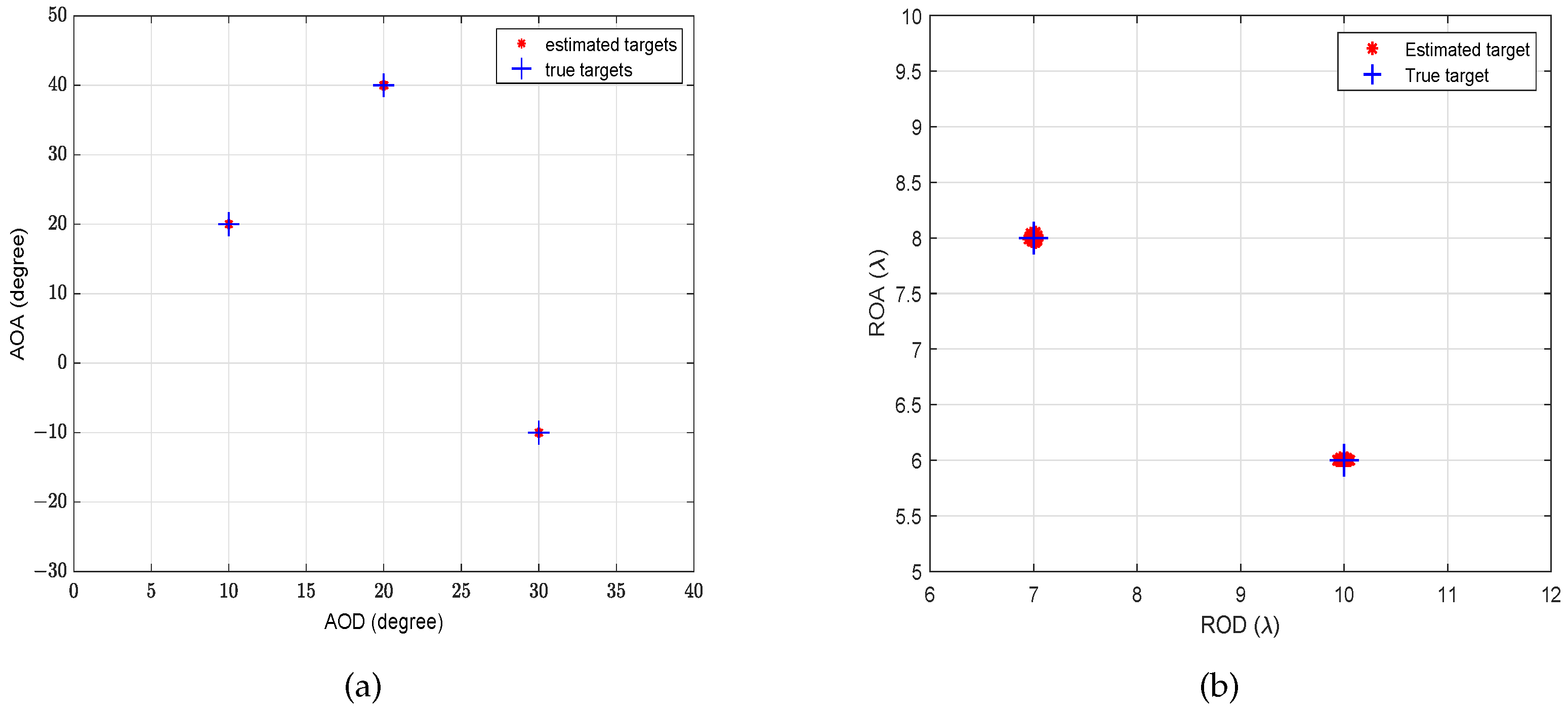
In this section, we perform numerical simulations to illustrate the performance of the proposed 4D parameter estimation algorithm. Consider bistatic MIMO arrays with $2M+1=21$$(M=10)$ transmit antennas and $2N+1=21$$(N=10)$ receive antennas, and each array is a symmetric ULA with spacing $d_t=d_r=\lambda /4$. Assume that there are $K=3$ targets, composed of an FF target and two NF targets. The three targets are located at $\left({\theta }_t,{\theta }_r,r_t,r_r\right)=\left({30}^{\circ },-{10}^{\circ },+\infty ,+\infty \right),\left({10}^{\circ },{20}^{\circ },10\lambda ,6\lambda \right),\left({20}^{\circ },{40}^{\circ },7\lambda ,8\lambda \right).$

First, we present the simulation results of the AOD and AOA for the mixed FF and NF targets and the ROD and ROA for the NF targets using the proposed algorithm. SNR is 15 dB and the number of snapshots is $L=100$. The result of 100 independent trials is shown in Figure 2. It is observed that the estimates of AOD and AOA for the three mixed FF and NF targets and the estimates of ROD and ROA for the two NF targets have high estimation accuracy and are close to their true values. In addition, the 4D parameters of AOD, AOA, ROD and ROA for multiple mixed targets can be well paired. The effectiveness of the proposed algorithm can be verified from the simulation.

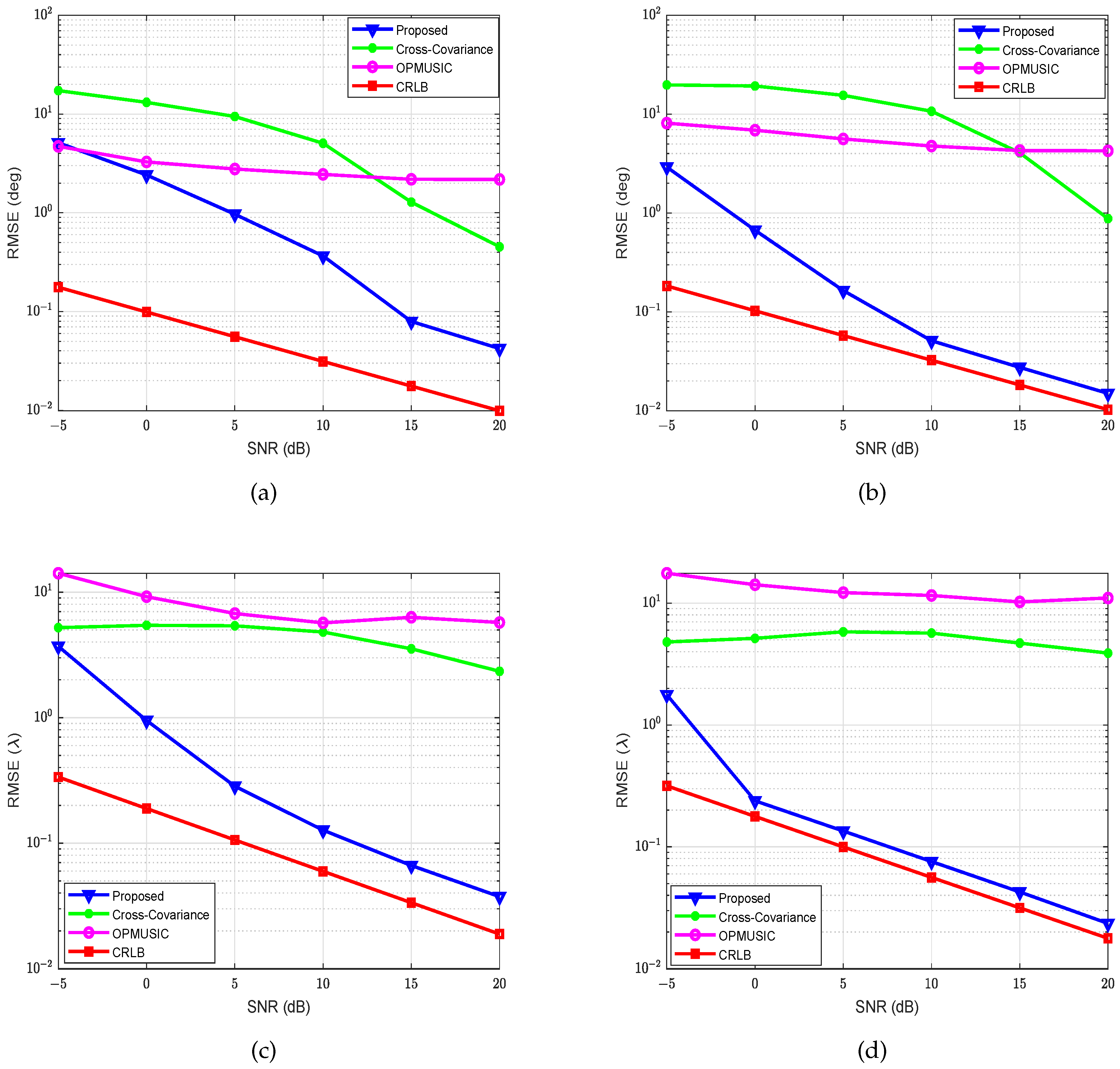
Next, we investigate the performance of RMSE versus SNR for 4D parameter estimation of AOD, AOA, ROD and ROA. The proposed tensor-based algorithm is compared with the Cross-Covariance algorithm in [15] and the OPMUSIC algorithm in [17], which we extend to 4D. Monte Carlo trials are used to compute the RMSE of ${\theta }_t$, $r_t$, ${\theta }_r$ and $r_r$. For example, the RMSE of ${\theta }_t$ can be calculated by

$${\mathrm{RMSE}}_{{\theta }_t}={\displaystyle \frac{1}{K}}\sum _{k=1}^K\sqrt{{\displaystyle \frac{1}{T}}\sum _{i=1}^T\left\{{({\widehat{\theta }}_{tk,i}-{\theta }_{tk})}^2\right\}}$$

(37)

where T represents the number of Monte Carlo trials. ${\widehat{\theta }}_{tk,i}$ denotes the estimated ${\theta }_{tk}$ in the ith Monte Carlo trial.

To show the superiority of our algorithm in a small number of snapshots, we set the number of snapshots as $L=5$. The SNR is varied from $-5$ dB to 20 dB. A total of 500 Monte Carlo trials are performed. The RMSE of AOD, AOA, ROD and ROA estimation versus SNR is plotted in Figure 3. As seen from Figure 3, with the increase in SNR, the proposed tensor-based algorithm can achieve much smaller RMSE and is close to CRLB. Also, it has smaller RMSE than the other two matrix-based algorithms. It implies that with the proposed algorithm, by using the covariance tensor and performing the HOSVD, the inherent multidimensional structure of the array data is well reserved. Therefore, the proposed tensor-based algorithm can achieve higher accuracy than the existing matrix-based algorithms for mixed FF and NF target localization, especially in a small number of snapshots.

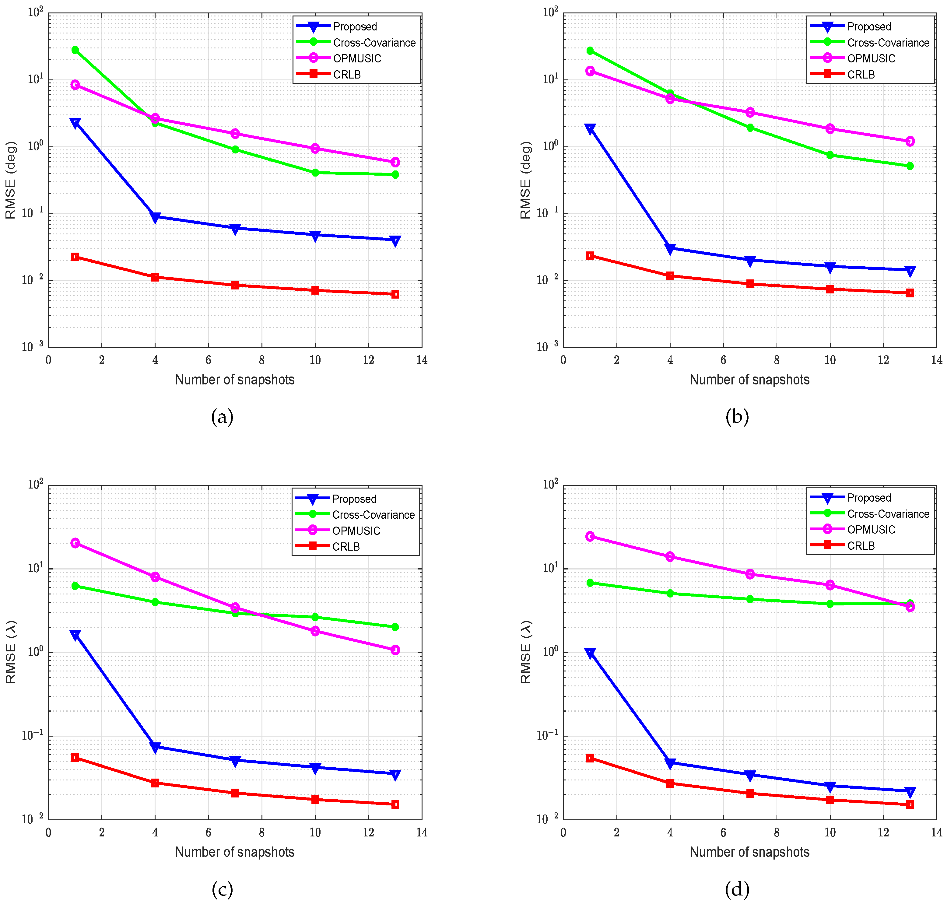
Next, we investigate the performance of RMSE versus the number of snapshots. The SNR is set as 15 dB. Also, a small number of snapshots is considered, which is varied from 1 to 13. The Monte Carlo trials is 500. The RMSE of AOD, AOA, ROD and ROA estimation versus the number of snapshots is shown in Figure 4. It reveals the similar results to the RMSE varying with SNR. The estimation accuracy of the proposed tensor-based algorithm is higher than that of the two other algorithms for all parameters, which implies that the multidimensional inherent structure of the tensor data is helpful for achieving a more accurate subspace estimation.

The simulation findings indicate that consolidating multidimensional data into structured matrices can lead to error accumulation and diminish the accuracy of multi-parameter estimation in mixed FF and NF target localization, particularly in scenarios with a limited number of snapshots. The proposed algorithm based on HOSVD can utilize the inherent multidimensional structure characteristics for the bistatic MIMO arrays, and have little damage to the original data structure.

Finally, as a supplementary experiment, we compare the running times of three algorithms and list the results in

Table 2. Comparison of the running time of three algorithms.

Method	Running Time (s)
Cross-Covariance algorithm	0.152716
OPMUSIC algorithm	30.318917
Proposed algorithm	0.965869

. The simulation conditions of the experiment are the same as those in Experiment 1. According to the experimental results, we can observe that the Cross-Covariance algorithm has the shortest running time, while the proposed algorithm takes slightly longer running time but still quickly provides estimation results. The OPMUSIC algorithm, on the other hand, has a very long running time, indicating poor real-time performance of the algorithm.

6. Conclusions

In this paper, we investigated the 4D parameter estimation of FF and NF targets using bistatic MIMO arrays and HOSVD. The proposed tensor-based algorithm shows an accuracy improvement from the fact that it can reserve the inherent multidimensional structure, especially in a small number of snapshots. The FF and NF targets can be well separated via range domain. Compared with the previous methods, the proposed solution provides a more robust performance of multiple-parameter estimation for mixed FF and NF target localization.

References

1. Xiao, M.; Mumtaz, S.; Huang, Y. Millimeter wave communications for future mobile networks. IEEE J. Sel. Areas Commun. 2017, 35, 1909–1935. [Google Scholar] [CrossRef]
2. Bjrnson, E.; Sanguinetti, L.; Wymeersch, H. Massive MIMO is a reality—What is next? Five promising research directions for antenna arrays. Digi. Signal Process 2019, 94, 3–20. [Google Scholar] [CrossRef]
3. Fang, Y.; Zhu, S.; Liao, B.; Li, X.; Liao, G. Target localization with bistatic MIMO and FDA-MIMO dual-mode radar. IEEE Trans. Aerosp. Electron. Syst. 2024, 60, 952–964. [Google Scholar] [CrossRef]
4. Ahmad, M.; Zhang, X.; Lai, X.; Ali, F.; Shi, X. Low-complexity 2D-DOD and 2D-DOA estimation in bistatic MIMO radar systems: A reduced-dimension MUSIC algorithm approach. Sensors 2024, 24, 2801. [Google Scholar] [CrossRef]
5. Shi, J.; Hu, G.; Zhang, X. Sparsity-based DOA estimation of coherent and uncorrelated targets with flexible MIMO radar. IEEE Trans. Veh. Technol. 2019, 68, 5835–5848. [Google Scholar] [CrossRef]
6. Xie, Q.; Pan, X.; Huang, M. Sparsity-based direction-of-departure and direction-of-arrival estimation for bistatic multiple-input multiple-output radar. IEEE Access 2019, 7, 118826–118838. [Google Scholar] [CrossRef]
7. Liu, D.; Zhao, Y.; Zhang, T. Sparsity-based two-dimensional DOA estimation for co-prime planar array via enhanced matrix completion. Remote Sens. 2022, 14, 4690. [Google Scholar] [CrossRef]
8. Zhang, R.; Shim, B.; Wu, W. Direction-of-arrival estimation for large antenna arrays with hybrid analog and digital architectures. IEEE Trans. Signal Process. 2021, 70, 72–88. [Google Scholar] [CrossRef]
9. Wei, X.; Jiang, Y.; Liu, Q. Calibration of phase shifter network for hybrid beamforming in mmWave massive MIMO systems. IEEE Trans. Signal Process. 2020, 68, 2302–2315. [Google Scholar] [CrossRef]
10. Elbir, A.M.; Mishra, K.V.; Chatzinotas, S. Spherical wavefront near-field DoA estimation in THz automotive radar. In Proceedings of the 18th European Conference on Antennas and Propagation (EuCAP), Glasgow, UK, 17–22 March 2024; pp. 1–5. [Google Scholar]
11. Wu, J.; Kim, S.; Shim, B. Near-field channel estimation for RIS-assisted wideband Terahertz systems. In Proceedings of the 2022 IEEE Global Communications Conference (GLOBECOM 2022), Rio de Janeiro, Brazil, 4 December 2022; pp. 3893–3898. [Google Scholar]
12. Singh, P.R.; Wang, Y.; Charge, P. Near field targets localization using bistatic MIMO system with symmetric arrays. In Proceedings of the 2017 25th European Signal Processing Conference (EUSIPCO), Kos, Greece, 28 August–2 September 2017; pp. 2403–2407. [Google Scholar]
13. Singh, P.R.; Wang, Y. Near field targets localization using bistatic MIMO system with spherical wavefront based model. In Proceedings of the 2017 25th European Signal Processing Conference (EUSIPCO), Kos, Greece, 28 August–2 September 2017; pp. 2408–2412. [Google Scholar]
14. Chen, C.; Zhong, W.D.; Yang, H. On the performance of MIMO-NOMA-based visible light communication systems. IEEE Photonics Technol. Lett. 2017, 30, 307–310. [Google Scholar] [CrossRef]
15. Hong, J.; Erning, H.Z.; Han, Q. 4-D Parameter Estimation in Bistatic MIMO Radar for Near-Field Target Localization. In Proceedings of the IEEE International Wireless Symposium (IWS), Shenzhen, China, 30 March–1 April 2015; pp. 1–4. [Google Scholar]
16. Zhao, T.; Chen, H.; Tian, Y. An algorithm for 5-D parameters estimation of near-field sources using parallel factor analysis. Multidimens. Syst. Signal Process. 2022, 33, 1139–1150. [Google Scholar] [CrossRef]
17. He, J.; Swamy, M.N.S.; Ahmad, M.O. Efficient application of MUSIC algorithm under the coexistence of far-field and near-field sources. IEEE Trans. Signal Process. 2012, 60, 2066–2070. [Google Scholar] [CrossRef]
18. Zheng, Z.; Fu, M.; Wang, W.Q. Mixed far-field and near-field source localization based on subarray cross-cumulant. Signal Process. 2018, 150, 51–56. [Google Scholar] [CrossRef]
19. Wang, K.; Wang, L.; Shang, J.R. Mixed near-field and far-field source localization based on uniform linear array partition. IEEE Sensors J. 2016, 16, 8083–8090. [Google Scholar] [CrossRef]
20. Ma, H.; Tao, H.; Xie, J. Mixed far-field and near-field source localization using a linear tripole array. IEEE Wirel. Commun. Lett. 2020, 9, 889–892. [Google Scholar] [CrossRef]
21. He, Q.; Cheng, Z.; Wang, Z. Mixed far-field and near-field source separation and localization based on FOC matrix differencing. Digit. Signal Process. 2022, 131, 103753. [Google Scholar] [CrossRef]
22. Zuo, W.; Xin, J.; Zheng, N. Subspace-based localization of far-field and near-field signals without eigendecomposition. IEEE Trans. Signal Process. 2018, 66, 4461–4476. [Google Scholar] [CrossRef]
23. Yang, J.; Hao, C.; Zheng, Z. Localization of mixed near-field and far-field multi-band sources based on sparse representation. Multidimens. Syst. Signal Process. 2020, 31, 173–190. [Google Scholar] [CrossRef]
24. Wang, B.; Liu, J.; Sun, X. Mixed sources localization based on sparse signal reconstruction. IEEE Signal Process. Lett. 2012, 19, 487–490. [Google Scholar] [CrossRef]
25. Wu, X.; Yan, J. Gridless mixed sources localization based on low-rank matrix reconstruction. IEEE Wirel. Commun. Lett. 2020, 9, 1748–1752. [Google Scholar] [CrossRef]
26. Huang, Z.; Wang, W.; Dong, F. A One-snapshot localization algorithm for mixed far-field and near-field sources. IEEE Commun. Lett. 2020, 24, 1010–1014. [Google Scholar] [CrossRef]
27. Huang, Z.; Xue, B.; Wang, W.; Dong, F.; Wang, D. A low complexity localization algorithm for mixed far-field and near-field sources. IEEE Commun. Lett. 2021, 12, 3838–3842. [Google Scholar] [CrossRef]
28. Tian, Y.; Lian, Q.; Xu, H. Mixed near-field and far-field source localization utilizing symmetric nested array. Digit. Signal Process. 2017, 73, 16–23. [Google Scholar] [CrossRef]
29. Wu, X. Localization of far-field and near-field signals with mixed sparse approach: A generalized symmetric arrays perspective. Signal Process. 2020, 175, 107665. [Google Scholar] [CrossRef]
30. Wu, X.; Zhu, W.-P. Single far-field or near-field source localization with sparse or uniform cross array. IEEE Trans. Veh. Technol. 2020, 69, 9135–9139. [Google Scholar] [CrossRef]
31. Su, X.; Hu, P.; Liu, Z.; Liu, T.; Peng, B.; Li, X. Mixed near-field and far-field source localization based on convolution neural networks via symmetric nested array. IEEE Trans. Veh. Technol. 2021, 70, 7908–7920. [Google Scholar] [CrossRef]
32. Zheng, Z.; Fu, M.; Wang, W.-Q.; So, H.C. Symmetric displaced coprime array configurations for mixed near- and far-Field source localization. IEEE Trans. Antennas Propag. 2021, 69, 465–477. [Google Scholar] [CrossRef]
33. Zhang, J.; Li, Y.; Qi, J.; Li, Y. Symmetric extended nested array for passive localization of mixture near-and far-field sources. IEEE Trans. Circuits Syst. II Express Briefs 2022, 70, 1244–1248. [Google Scholar] [CrossRef]
34. Wu, X.; Yan, J. 3-D Mixed far-field and near-field sources localization with cross array. IEEE Trans. Veh. Technol. 2020, 69, 6833–6837. [Google Scholar] [CrossRef]
35. Chen, H.; Ahmad, F.; Vorobyov, S.V.; Porikli, F. Tensor decompositions in wireless communications and MIMO radar. IEEE J. Sel. Top. Signal Process. 2021, 15, 438–453. [Google Scholar] [CrossRef]
36. Mao, C.; Shi, J.; Wen, F. Target localization in bistatic EMVS-MIMO radar using tensor subspace method. IEEE Access 2019, 7, 163119–163127. [Google Scholar] [CrossRef]
37. Xu, F.; Yang, X.; Lan, T. Search-free direction-of-arrival estimation for transmit beamspace multiple-input multiple-output radar via tensor modeling and polynomial rooting. IET Radar Sonar Navig. 2021, 15, 574–580. [Google Scholar] [CrossRef]
38. Xu, F.; Morency, M.W.; Vorobyov, S.A. DOA estimation for transmit beamspace MIMO radar via tensor decomposition with vandermonde factor matrix. IEEE Trans. Signal Process. 2021, 70, 2901–2917. [Google Scholar] [CrossRef]
39. Shi, J.; Wen, F.; Liu, T. Nested MIMO radar: Coarrays, tensor modeling, and angle estimation. IEEE Trans. Aerosp. Electron. Syst. 2021, 57, 573–585. [Google Scholar] [CrossRef]
40. Singh, P.R.; Wang, Y.; Charge, P. Bistatic MIMO radar for near field source localization using PARAFAC. Electron. Lett. 2016, 52, 1060–1061. [Google Scholar] [CrossRef]
41. Kolda, T.G.; Bader, B.W. Tensor decompositions and applications. SIAM Rev. 2009, 51, 455–500. [Google Scholar] [CrossRef]
42. Lathauwer, L.D.; Moor, B.D.; Vandewalle, J. A multilinear singular value decomposition. SIAM J. Matrix Anal. Appl. 2000, 21, 1253–1278. [Google Scholar] [CrossRef]
43. Barrar, R.B.; Wilcox, C.H. On the fresnel approximation. IRE Trans. Antennas Propag. 1958, 6, 43–48. [Google Scholar] [CrossRef]
44. Stoica, P.; Nehorai, A. Performance study of conditional and unconditional direction-of-arrival estimation. IEEE Trans. Acoust. Speech Signal Process. 1990, 38, 1783–1795. [Google Scholar] [CrossRef]
45. Pesavento, M.; Gershman, A.B. Maximum-likelihood direction-of-arrival estimation in the presence of unknown nonuniform noise. IEEE Trans. Signal Process. 2001, 49, 1310–1324. [Google Scholar]
46. Stoica, P.; Larsson, E.G.; Gershman, A.B. The stochastic CRB for array processing: A textbook derivation. IEEE Signal Process. Lett. 2001, 8, 148–150. [Google Scholar] [CrossRef]
Figure 1. Bistatic MIMO array configuration.
Remotesensing 16 03366 g001
Figure 2. Simulation results with the proposed algorithm for (a) AOD and AOA estimation and (b) ROD and ROA estimation. S N R = 15 dB, M = 10 , N = 10 , K = 3 , L = 100 , and 100 independent trials. θ t , θ r , r t , r r = 30 , 10 , + , + , 10 , 20 , 10 λ , 6 λ , 20 , 40 , 7 λ , 8 λ . .
Remotesensing 16 03366 g002
Figure 3. Performance of RMSE versus SNR for different algorithms. (a) AOD estimation, (b) AOA estimation, (c) ROD estimation, (d) ROA estimation. L = 5 , M = 10 , N = 10 , K = 3 , and 500 Monte Carlo trials. θ t , θ r , r t , r r = 30 , 10 , + , + , 10 , 20 , 10 λ , 6 λ , 20 , 40 , 7 λ , 8 λ .
Remotesensing 16 03366 g003
Figure 4. Performance of RMSE versus the number of snapshots for different algorithms. (a) AOD estimation, (b) AOA estimation, (c) ROD estimation and (d) ROA estimation. M = 10 , N = 10 , K = 3 , S N R = 15 dB and 500 Monte Carlo trials. ( θ t , θ r , r t , r r ) = ( 30 , 10 , + , + ) , ( 10 , 20 , 10 λ , 6 λ ) , ( 20 , 40 , 7 λ , 8 λ ) .
Remotesensing 16 03366 g004