Article

Development and Comparison of InSAR-Based Land Subsidence Prediction Models

by
Lianjing Zheng
1,
Qing Wang
1,
Chen Cao
1,*,
Bo Shan
2,
Tie Jin
1,
Kuanxing Zhu
1 and
Zongzheng Li
1
1
College of Construction Engineering, Jilin University, Changchun 130022, China
2
China Power Engineering Consulting Group, Northeast Electric Power Design Institute Co., Ltd., Changchun 130021, China
*
Author to whom correspondence should be addressed.
Remote Sens. 2024, 16(17), 3345; https://doi.org/10.3390/rs16173345
Submission received: 1 August 2024 / Revised: 30 August 2024 / Accepted: 3 September 2024 / Published: 9 September 2024
(This article belongs to the Topic Environmental Geology and Engineering)

Abstract

:
Land subsidence caused by human engineering activities is a serious problem worldwide. We selected Qian’an County as the study area to explore the evolution of land subsidence and predict its deformation trend. This study utilized synthetic aperture radar interferometry (InSAR) technology to process 64 Sentinel-1 data covering the area, and high-precision and high-resolution surface deformation data from January 2017 to December 2021 were obtained to analyze the deformation characteristics and evolution of land subsidence. Then, land subsidence was predicted using the intelligence neural network theory, machine learning methods, time-series prediction models, dynamic data processing techniques, and engineering geology of ground subsidence. This study developed three time-series prediction models: a support vector regression (SVR), a Holt Exponential Smoothing (Holt) model, and multi-layer perceptron (MLP) models. A time-series prediction analysis was conducted using the surface deformation data of the subsidence funnel area of Zhouzi Village, Qian’an County. In addition, the advantages and disadvantages of the three models were compared and analyzed. The results show that the three developed time-series data prediction models can effectively capture the time-series-related characteristics of surface deformation in the study area. The SVR and Holt models are suitable for analyzing fewer external interference factors and shorter periods, while the MLP model has high accuracy and universality, making it suitable for predicting both short-term and long-term surface deformation. Ultimately, our results are valuable for further research on land subsidence prediction.

1. Introduction

Land subsidence caused by human activities is a serious problem worldwide [1,2,3], and it is crucial to slow down severe cases (subsidence rate > 3 cm/year) [4]. Land subsidence is primarily caused by the excessive extraction of groundwater from aquifers, leading to water depletion [5,6]. The over-exploitation of groundwater beyond natural recharge limits can result in various disasters, including lowered groundwater levels, seawater intrusion, deteriorated groundwater quality, land subsidence, poor drainage, and flooding [7,8].
To address the key issues of evaluating and predicting land subsidence, numerous studies have been conducted and can be categorized into two main types [1]: (1) those focused on the physical mechanism of land subsidence, primarily surface subsidence caused by resource exploitation; (2) those that establish fitting mathematical models to predict subsidence trends using extensive measured data. Studies of the first category estimate subsidence by simulating physical evolution processes using methods such as the finite element [9,10], difference [11], and numerical analysis methods based on Biot’s consolidation theory [12,13]. Models of the second category include the logistic curve equation [14] and the Weibull [15] and hyperbolic [16] models. However, these models have limitations in practical application since they cannot accurately reflect the entire land subsidence process.
Theoretical analysis and model tests are important for studying land subsidence mechanisms [17]. Physical prediction models, which incorporate factors influencing land subsidence, simulate the subsidence process and effectively explain its mechanisms [18]. However, these models require extensive hydrological data, which limits their applicability [19]. In contrast, mathematical prediction models use mathematical functions to represent the statistical characteristics of historical land subsidence [20]. These models have a broader range of applications than physical prediction models [21,22]. However, when land subsidence values vary widely, the prediction performance of mathematical models is low [23]. This is because mathematical models cannot explain the underlying mechanisms of land subsidence.
With the development of artificial intelligence, machine learning-based models for predicting land subsidence can combine the strengths of both physical and mathematical models while overcoming their limitations [24,25,26] and provide more reliable prediction results [27,28,29,30]. Chen et al. [31] used a random forest (RF) algorithm and geographical detector (GD) technology to quantitatively analyze the impact of different aquifers on land subsidence in 2020. This method combines the advantages of machine learning and the characteristics of geospatial data, providing a new perspective on the complex relationship between groundwater levels and land subsidence. Rajabi et al. [32] established a numerical model in 2018 to assess the impact of aquifer changes on land subsidence in the Aliabad plain, Iran. Ali et al. [33] used two regression estimation methods with weighted land subsidence characteristics to predict land subsidence in Taiwan in 2020. Ding et al. [34] analyzed and predicted land subsidence by establishing a linear engineering settlement numerical model in 2020. Although numerical models may have some uncertainties when simulating the settlement process in real-world engineering environments, they still provide a valuable tool for understanding and predicting land subsidence. Among machine learning methods, the BP neural network (BPNN) is effective for quantitatively predicting the nonlinear relationship between land subsidence and groundwater levels [35,36]. Wang et al. [37] studied the thermal conductivity characteristics of different soil types and discovered that the thermal conductivity and resistivity of soil are nonlinear when saturated. They utilized the MLP neural network’s ability to effectively handle nonlinear data to predict the soil’s thermal resistance coefficient. Huang et al. [38] proposed that the factors influencing agricultural droughts are both large in volume and nonlinear via agricultural drought monitoring, prediction, and risk assessment. They also used deep learning combined with information fusion to predict nonlinear data, further improving the accuracy of regional agricultural drought monitoring and prediction. However, adjusting the algorithm’s parameters is cumbersome, and the calculations are large and time-consuming. The random forest (RF) algorithm [39,40], as an integrated algorithm, performs well with its default parameters. This makes it more efficient and practical for analyzing the relationship between land subsidence and groundwater level.
However, existing prediction models and methods ignore the impact of the non-stationary spatiotemporal relationship between influencing factors and cumulative ground subsidence, leading to poor accuracy in predicting ground subsidence deformation. Masoud M. et al. [41] used PMWIN5.3 (MODFLOW for Windows) to develop a numerical simulation for characterizing ground subsidence in the southwest plain of Tehran and predicted its trend until 2018. Yonghao Yuan et al. [30] proposed a geographical and time-weighted regression method combining long short-term memory (LSTM) with a multivariate approach and an attention mechanism (GTWR-LSTMm-AM) to accurately predict ground subsidence over time. Although time-series data prediction is widely applicable, its accuracy can be limited by the amount of available data [42,43].
This study used SBAS-InSAR to extract surface deformation characteristics from Sentinel-1 images covering the study area. This approach relies on synthetic aperture radar to provide high-precision temporal and spatial resolution measurements of regional deformation. With a sufficient volume of Sentinel-1 data, subsidence information from overlapping areas was processed and then interpolated for use in training and learning prediction models. We innovatively combined theories from artificial intelligence neural networks, machine learning methods, common time-series prediction models, measurement adjustment and dynamic data processing, and engineering geological subsidence to predict ground subsidence using InSAR with three different time-series models. After analyzing the predicted deformation, we further evaluated the errors and practical effectiveness of these three models in predicting surface deformation.

2. Study Area

Qian’an County is located northwest of Jilin Province (Figure 1a,b) and west of Songyuan City, with a north latitude of 44°37′47″–45°18′08″ and east longitude of 123°21′16″–124°22′50″. It is also in the middle of the Yuechi fault depression basin, which is a subsidence area from the Mesozoic Era, with an altitude of 120 m–187.5 m; the terrain gradually rises from the northeast to southwest, with prominent alluvial and lacustrine plains from sediment accumulation. The area is also in the center of the Songliao depression and is characterized by a graben formed during the Hercynian movement, on which a thick layer of Cretaceous strata is deposited. Subsequently, the basal differential movement of the Yanshan movement formed a west-dipping monocline structure and two anticlines, namely Dalai-Heidi Miao Changyuan and Chaganor Changyuan. The entire area is extensively covered by quaternary strata, with tertiary and Cretaceous strata underlain.
The main lithologies in the study area are silty sub-clay, sandy loam, sub-clay, gravel-bearing clay, mudstone, thin sandstone, and clastic rock. The surface water in this area is scarce, and the groundwater types mainly include quaternary loose rock pore water and Neogene clastic rock fissure-pore water. The quaternary pore-confined water aquifer is shallow in the south and southwest of the study area, about 20~50 m, and the rest is mostly greater than 50 m; the aquifer mainly comprises sand and gravel of the Baitushan Formation. The confined water of the tertiary clastic rocks is widely distributed throughout the whole county, and the sandstone and conglomerate aquifer groups are overlapped by two layers of the Da’an and Taikang Formations, which are stable in layer, large in thickness, and sufficient in water richness. The pore fissures of the Taikang Formation are confined to water, and this layer is generally developed in this area and buried 25~108 m below the ground. The fissure-pore confined water of the Da’an Formation is widely distributed throughout the whole area, the aquifer thickness is 18~53 m, and the confined water level is generally 6.56~7.08 m from the ground. The water richness of aquifers varies greatly. Qian’an County mainly takes the confined water of the quaternary and Neogene Taikang Formation.
Qian’an County has a mid-temperate arid and semi-arid continental monsoon climate, with an average annual temperature of 4.6 °C. The highest and lowest recorded temperatures are 37.8 °C and −34.8 °C, respectively. The average annual precipitation is 417 mm, with over 80% between June and September. The annual maximum and minimum precipitations are 686 mm and 213.9 mm, respectively. The area is also subject to peak accelerations within the range of 190l (equivalent to an intensity of VIII), making it one of the few high-intensity seismic zones in northeastern China.

3. Data and Methods

3.1. Data

This study used data from two SLC Level 1 product images in the interferometric wide-swath (IW) mode of the Sentinel-1 satellite to conduct model-related prediction analysis. The image coverage is shown in Figure 1c, ranging from January 2017 to December 2021, with a total of 64 periods. Detailed information on the used SAR images is presented in Table 1. The average incident angles of the radar for the two images are 36.02° and 36.94°. Sentinel-1 is a C-band satellite with a wavelength of 5.6 cm, an orbital altitude of approximately 700 km, and a revisit period of 12 days. It has a large-scale spatial coverage of approximately 250 km and a resolution of 5 m × 20 m. It can provide high-resolution monitoring of global land and sea surfaces in a multi-polarized manner. These SAR data are processed using SBAS-InSAR to obtain millimeter-level surface deformation data on the study area.

3.2. Methodology

The townships under the jurisdiction of Qian’an County, Daya Livestock Farm, Scale Characteristic Agricultural Park, and Tengzi Plantation Farm are densely distributed areas of personnel and property, and many major production engineering facilities are distributed here. Disasters such as surface structure destructions caused by land subsidence have affected the safety of people’s lives and property, and land subsidence is a slow-changing geological disaster that makes repair difficult and will continue to deform and damage in the future, so it is necessary to predict land subsidence deformation in typical areas to reduce safety risks. The subsidence funnel of Zhouzi Village in Yuzi Township was selected as the research object, and the SAR data were processed via SBAS-InSAR technology to obtain the surface deformation information of the study area. Then, the deformation data were preprocessed, with abnormal data eliminated after deviation calculation, and Gaussian interpolation was applied to the data to ensure their applicability in the three prediction models.

3.2.1. Data Preprocessing

(1)
Abnormal Data Elimination
We used sliding windows to analyze distribution characteristics and detect and eliminate gross errors. A gross error is defined as an observation value where the difference between the sliding window and the local median exceeds three times the scaled median absolute deviation (SMAD), which is calculated as follows [44]:
S M A D = C m e d i a n ( S i m e d i a n ( S ) ) ,   C = 1 / ( s q r t ( 2 ) e r f c i n v ( 3 / 2 ) )
(2)
Gaussian interpolation processing of the time series data
The Gaussian interpolation algorithm uses prior information to approximate time-series deformation data with a Gaussian distribution. It interpolates the second-largest value in the neighboring cells using the maximum amplitude and value of the shape variable in the distance cell. Let the probability density function of the Gaussian distribution [45] be
f ( t ) = 1 2 π σ 2 exp ( ( t t 0 ) 2 2 σ 2 )
where t0 and σ2 are the mean and variance of the Gaussian distribution, respectively.

3.2.2. Prediction Model

This study used support vector regression (SVR), Holt’s exponential smoothing (HOLT) model (proposed by Holt in 1957), and multi-layer perceptrons (MLPs) to create land subsidence prediction models. The principles of these methods are elucidated below.
(1)
Support Vector Regression (SVR)
Support vector regression (SVR) is an algorithm designed for regression problems using support vector methods [46]. Its basic principle involves training the model to position data samples between two parallel lines, minimizing the total deviation of all points from these lines. The goal is to find the maximum distance between these two lines, which represents the optimal hyperplane for the SVR model.
For a given dataset {x1, x2, …, xn} and its corresponding actual values {y1, y2, …, yn}, the goal is to obtain a regression formula such that f(x) is as close to the actual y value as possible. The weight vector w and offset B must be determined to achieve this, with φ(x) representing a nonlinear mapping. By introducing relaxation variables, the ε - SVR problem is transformed into a quadratic programming problem as follows:
min 1 2 w 2 + C i = 1 m ( ξ i + ξ i * )
s . t .   f ( x i ) y i ε + ξ i
y i f ( x i ) ε + ξ i *
ξ i 0 ,   ξ i * 0 , i = 1 , 2 , , m ,
where C is the control penalty parameter; min 1 2 w 2 is the control item of a complex function; ξ i and ξ i * are the relaxation variables; and ε is the insensitive loss factor. The dual problem of SVM can be obtained by introducing a Lagrange multiplier as follows [47]:
max α , α * i = 1 m ( α i * α i ) y i i = 1 m ( α j * + α j ) ε 1 2 i = 1 m j = 1 m ( α i * α i ) ( α j * α j ) K ( x i , x j )
where α i , α i * , α j , and α j * are Lagrange multipliers, and K ( x i , x j ) is the kernel function. The regression function can be obtained by solving the above equation as follows:
f ( x ) = i = 1 m ( α i * α i ) K ( x i , x j ) + b
(2)
Holt’s Exponential Smoothing Model
Holt’s exponential smoothing model was proposed by Holt in 1957 [48]. It differs from the general exponential smoothing model in that it directly smooths the trend data and predicts the original time series. The model assumes that all known data impact the predicted value. The short-term data have a greater impact on the predicted value, while the long-term data have a smaller impact on the predicted value, and the impact decreases in geometric progression, as demonstrated below [49]:
S t = α X t + ( 1 α ) ( S t 1 + T t 1 )  
T t = γ ( S t S t 1 ) + ( 1 γ ) T t 1
X t + m = S t + m T t
where St and St−1 represent the estimation of the trend; Tt and Tt1 represent the estimation of the trend increment of t and t − 1, respectively; a and γ are the smoothing parameters, with 0 ≤ α ≤ 1 and 0 ≤ γ ≤ 1; Xt is the observation value of the t period; Xt + m is the prediction value of the t + m period; and m is the prediction extrapolation period.
(3)
Multi-layer perceptron (MLP) model
The multi-layer perceptron (MLP) model is a classic feedforward neural network model [50]. The first layer of the MLP is the input layer, and the number of input layers is the number of factors affecting the output parameters. The last layer is the output layer, and the rest are hidden. The specific process is shown in Figure 2. The network uses neurons as the smallest unit, and the output of the previous layer is the input of the next layer. The input information of multiple nodes is finally nonlinearly mapped to a single output on the output layer.
Assuming the weight matrix Wk and intercept matrix Bk are given, consider an MLP model with one hidden layer, which consists of an input layer, a hidden layer, and an output layer. If the number of input parameters is n, and x represents the output node value, the output sj value of the hidden layer can be calculated using Equation (12).
The value of j is taken from 1 to m, which represents the number of hidden layer nodes. The final output o is determined using Equation (13).
s j = f ( i = 1 n ( ω i j x i ) b j )
o = f ( i = 1 m ( ω i s t ) b )
In Equation (13), there are m hidden nodes and one output node; the elements in the weight matrix are represented as ωl. The bias matrix only contains one intercept term b. The values of the weight matrix Wk and the intercept matrix Bk are large. The weight matrix Wk and the intercept matrix Bk are crucial as they directly determine the final output o. As the MLP structure becomes more complex, it involves more input parameters, hidden nodes, and layers.

4. Results and Discussion

4.1. Deformation of Typical Subsidence

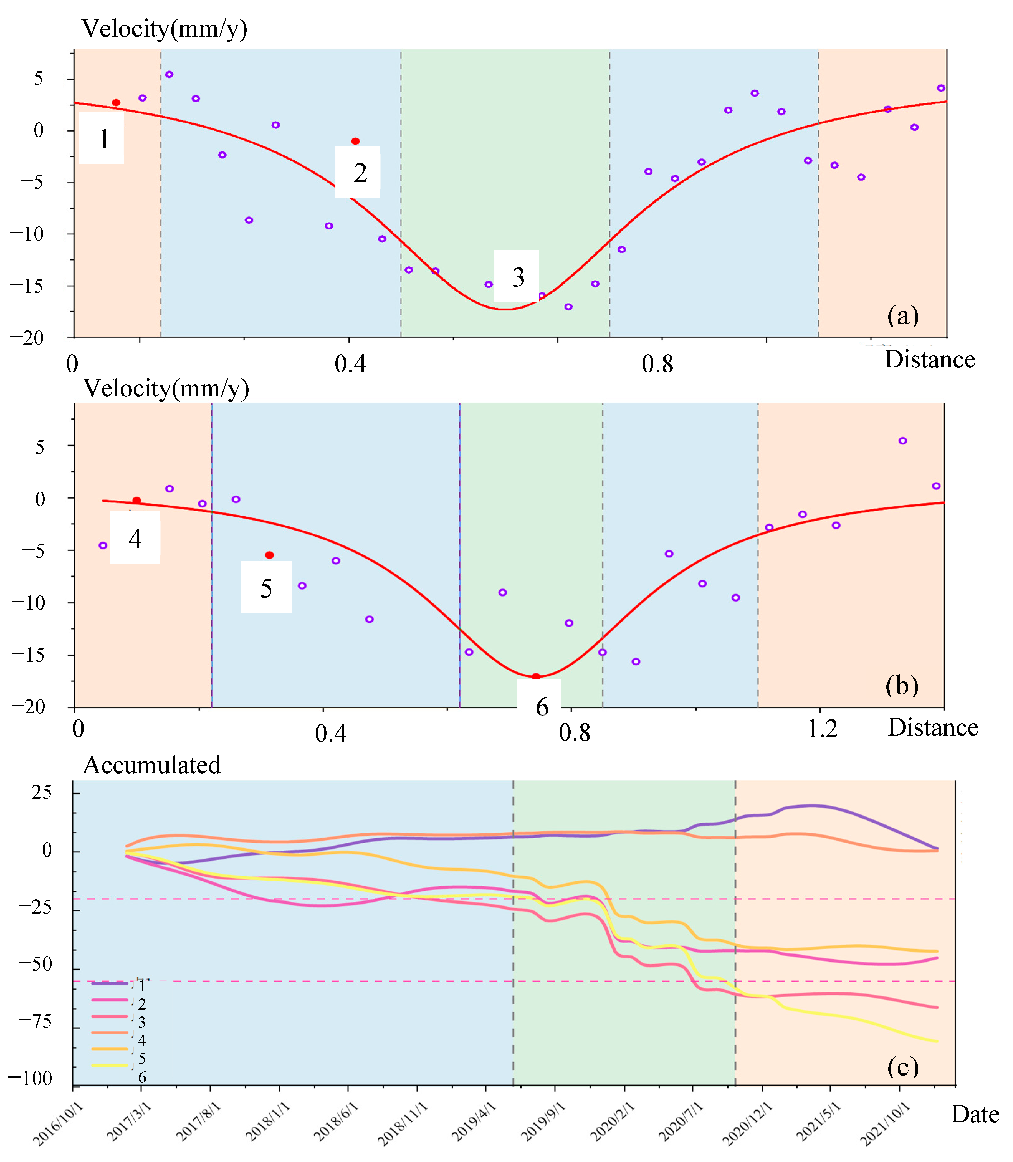
In this study, we focused on the settlement funnel of Zhouzi Village, which exhibited typical settlement characteristics, for predictive research using surface deformation data from Sentinel-1. The data span from January 2017 to December 2021. The time-series cumulative settlement data for this location, based on Sentinel-1 observations, are shown in Figure 3, with deformation rates ranging from −20 mm/y to 20 mm/y. Among them, over 80% of the points show a downward trend at locations far from the settlement center due to the influence of vegetation growth and errors, but a few points showed upward trends. Based on the monitoring results of InSAR, we conducted a detailed on-site investigation in Zhouzi Village. The funnel showed typical subsidence characteristics, with obvious ground fissures and surface subsidence phenomena, which were highly consistent with the InSAR results, confirming the accuracy of the monitoring results, which can be used for subsequent model prediction.
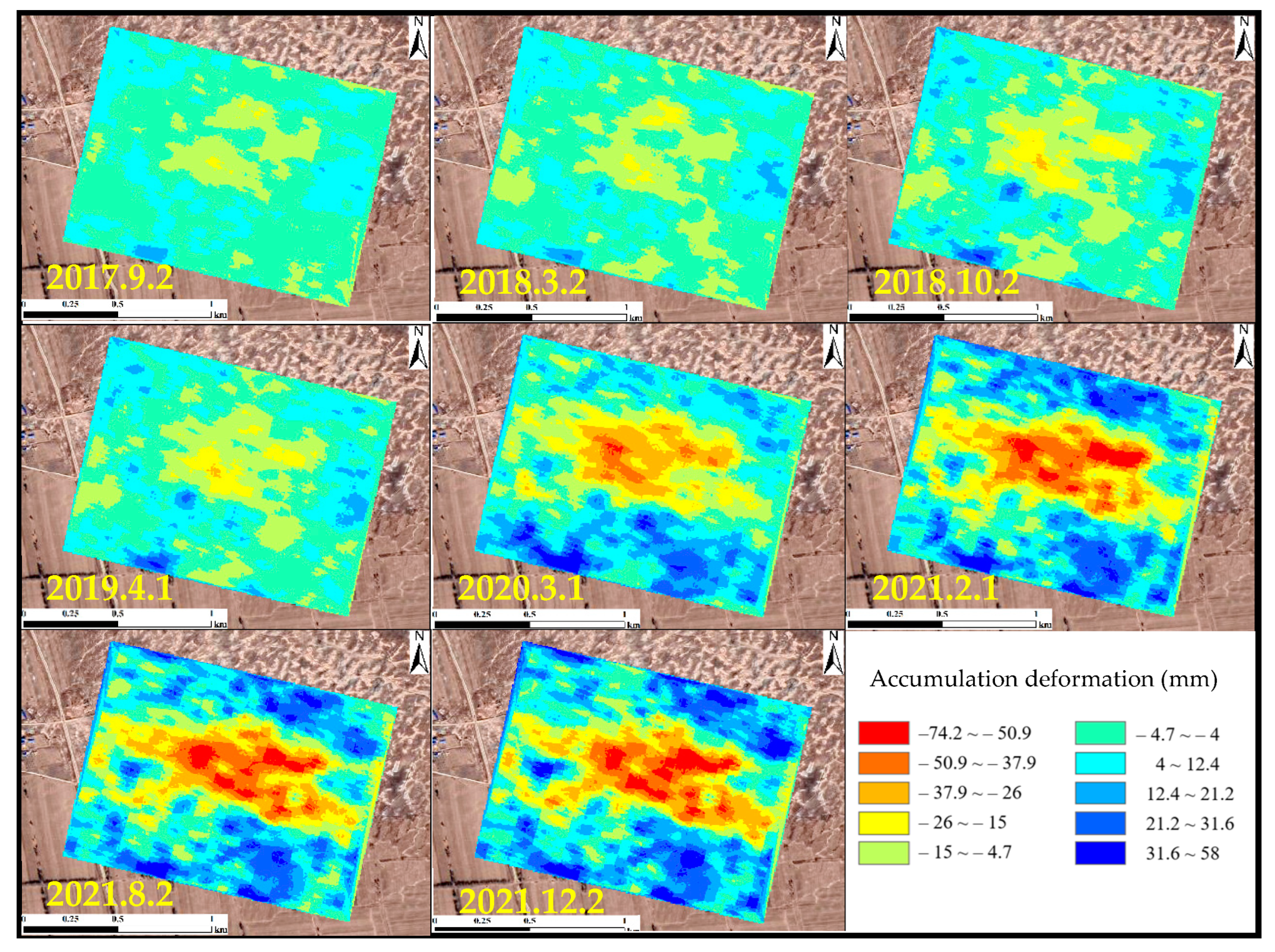
The maximum settlement deformation rate of the settlement funnel in Zhouzi Village ranges from −15 mm to −20 mm per year. The cumulative deformation results of Zhouzi Village were interpolated, and the representative settlement results were selected as shown in Figure 4.
Over the past four years, from the perspective of value and range, the deformation of the settlement funnel has gradually increased, and the maximum deformation has reached −74.2 mm. We used time-series data from 1078 subsidence points within the subsidence funnel to ensure the availability and universality of the ground subsidence prediction model. These data were processed by removing anomalies and applying Gaussian interpolation before making predictions. We selected six representative coherent points at the intersection of two profiles in the following areas for detailed research: the edge of the mobile basin, dangerous movement, and fault. Figure 3 presents two cross-sectional lines of the settlement funnel and the locations of six typical coherent points. Figure 5a–c presents the time-series deformation trend in six selected coherence points. The horizontal axes in Figure 5a,b represent the distances from A to A ‘and B to B’ in the settling funnel, while the vertical axes represent the deformation rate at each point on the profile line. The results indicate significant differences in deformation at each point, with uneven deformation at each point. The maximum deformation rate can reach about −17 mm/y, and the deformation degree gradually increases from both sides of the basin to the middle, forming a funnel shape. Figure 5c reflects the temporal deformation of six coherent points. From January 2017 to May 2019, most of the coherent points are in the stage of uniform deformation, showing small deformation. From May 2019 to December 2020, except for points 1 and 4, there is a trend in accelerated deformation. Afterwards, the coherent points gradually became uniformly deformed.

4.2. Time Series Deformation Prediction of the Overall Settlement Funnel Area

A total of 1078 settlement points were obtained in the settlement funnel of Zhouzi Village via SBAS-InSAR processing, and each point covered 64 periods of surface subsidence information. However, the 64-period data are not evenly distributed at the same time interval, which hinders the operation of the prediction model. Therefore, Gaussian interpolation is used to interpolate the deformation data into 256 periods with equal time intervals. A total of 256 samples were obtained using the deformation information and latitude and longitude coordinates of each point in each period as input values to form an experimental sample. The top 80% were selected for the training set, and the bottom 20% were used for validation analysis.
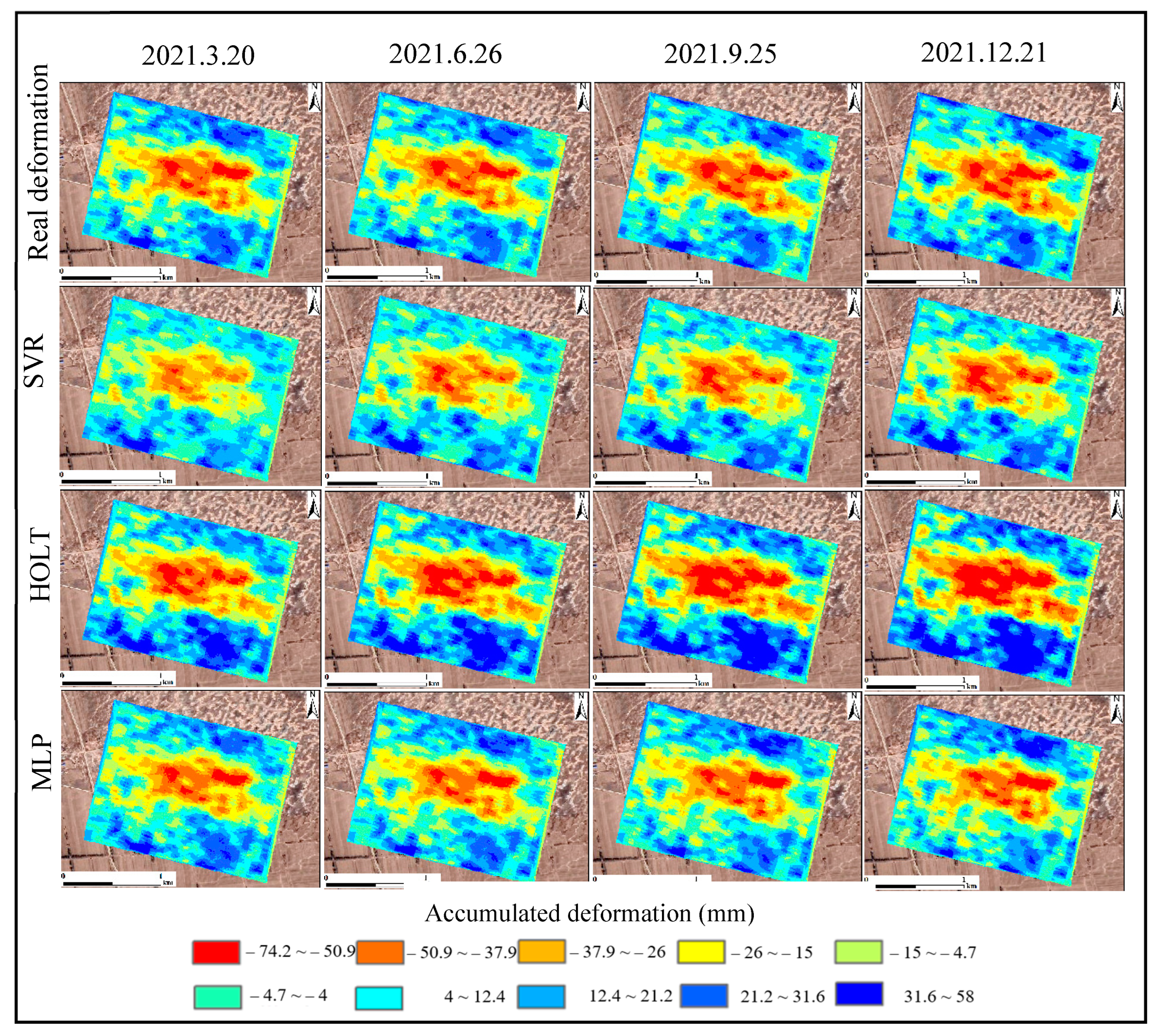
Both the predicted and measured deformation ranges from −74.2 mm to 58 mm formed significant subsidence funnels in the central area. Groundwater extraction in Qian’an County, mainly irrigated farmland and land subsidence characteristics, regularly changed due to seasonal changes. During the rainy season, farmland is irrigated from rainfall, which reduces groundwater withdrawal and replenishes the groundwater table, resulting in a significant slowdown in the surface decline rate. During the rainfall period, the surface rises significantly and sinks during the dry season. According to Figure 6, on 21 December 2021, the measured data show that the severely subsiding region (deformation ranging from −74.2 mm to −37.9 mm) accounted for about 9.8% of the total study area, and the deformation degree predicted from the SVR model was relatively small. The severely subsiding region accounted for about 9.8% of the total study area, and a considerable number of deformation points underwent significant subsidence, but this is not reflected in Figure 6.
The results of the HOLT model were opposite to those of the SVR model, predicting a larger deformation degree over the entire area, with the severely subsiding region accounting for about 15% of the total study area. Consequently, the HOLT model tends to overestimate deformation, predicting severe subsidence even for many points that have not actually undergone significant subsidence. As a result, areas that have not experienced severe subsidence are also classified as such. Overall, the predicted severely subsiding regions account for about 10% of the total study area. Compared with the previous two models, the MLP model is closer to the measured results for both deformation degree and range.
Figure 7 shows the Mean Absolute Error (MAE) values of the overall subsidence leakage area as outputs via the decoding modules in the three prediction models. It also displays the MAE distribution between the predicted deformation of the subsidence funnel area in Zhouzi Village and the actual deformation data based on SBAS-InSAR.
On 20 March 2021, the MAE values of the three models were all less than 10. When comparing the MAE values obtained from the three different models horizontally, the MLP model had the smallest prediction error, followed by the HOLT model, and the SVR model had the largest prediction error.
On 26 June 2021, the error values of the SVR and HOLT models increased significantly compared to the previous period, with error values ranging from 10 to 20, accounting for about half of the area. The error values of the MLP model showed almost no increase compared to the previous period. The areas where the error values of the three models increased rapidly were also mainly located in the areas with higher error values in the previous period. Among the three models, MLP had the smallest prediction error.
On 25 September 2021, the prediction errors of the SVR and HOLT models increased further over time, with most regions reaching MAE values in the range of 10–20 and some in the range of 20–30. The prediction errors of the MLP model increased slightly over time, with a few regions reaching the range of 10–20. Regions that had higher errors continued to show the fastest error growth rates for all three models. Overall, the MLP model still had the lowest prediction errors compared to the other two models.
On 21 December 2021, the errors of the SVR and HOLT models increased further, while the prediction error of the MLP model increased slightly; however, the error in most areas was still less than 10.
The prediction error values of the three models present different distribution patterns over time. With time, the prediction error values of the overall regional time-series surface deformation data in Zhouzi Village gradually increased. The areas with faster error growth rates were primarily those with higher initial prediction errors. The error growth rates of the SVR and HOLT models were faster than the MLP model. As of 26 June 2021, the predicted deformation values of the SVR and HOLT models still possessed a certain degree of accuracy, but as the prediction time increased, the error gradually increased, and the predicted deformation values of these two models presented a significant deviation from the measured results. The short- and long-term prediction results of the MLP model are more accurate. The predicted deformation values provided by the MLP model are more accurate and suitable for predicting surface deformation in the study area.

4.3. Temporal Deformation Prediction of the Coherent Points

This section provides a detailed discussion of the predicted deformation and error values for six representative coherent points selected from Section 4.1; the specific locations of the six points are shown in Figure 3. It also covers the time-series data, showing variations in the predicted deformation values and errors throughout the prediction process, as shown in Figure 8.
The measured cumulative deformation from 26 December 2020, to 21 December 2021, obtained via InSAR for six coherent points (points 1–6) ranges from 2 to 20 mm, −52 to −42 mm, −60 to −65 mm, 1 to −8 mm, −42 to −40 mm, and −80 to −62 mm. The subsidence rate and deformation range of the coherent points at different locations selected on different sections of the moving basin vary significantly.
The measured deformation values at points 1, 3, and 4 and the deformation values predicted using the three prediction methods showed a trend in first increasing slightly and then decreasing. The error values of the SVR and HOLT models gradually increased, while the error values of the MLP model changed slightly. The MLP model’s predictions for deformation values at points 1, 3, and 4 closely matched the measured results. For points 2 and 6, both the measured deformation values and those predicted using all three models showed a downward linear trend. The deformation values predicted using the three methods for point 2 were relatively close to the measured data, and the MLP model provided predictions for point 6 that were the closest to the measured results.
At point 5, the measured deformation was much smaller than that predicted using the HOLT and MLP models, with almost no actual deformation observed. The deformation predicted using the SVR model shows a downward linear trend. The error values of the three models gradually increase, with the SVR model showing a faster growth rate, while the HOLT and MLP models show a smaller change in error values. The HOLT and MLP models predict deformation at point 5 in a time series that fits the measured results.
After comparing the measured results of these six typical coherent points with the predicted time-series surface deformation values and analyzing the time-series variation in error values, we found significant differences in the subsidence rates and deformation ranges among the coherent points selected from different locations on various sections of the moving basin. The performance of the three models in predicting the time-series deformation at these six typical coherent points also varied. The deformation values at the six typical coherent points predicted using the SVR and HOLT models generally presented linear or simple function curve changes. For individual points with uneven subsidence rates or irregular changes such as first rising and then subsiding, accurate predictions cannot be made. The MLP model has higher accuracy in predicting nonlinear time-series data based on the ability of multi-layer neural layers to extract complex features through layer-by-layer connections.

4.4. Discussion

The error distribution obtained from the prediction models was analyzed. Over time, the error values of the three prediction models for predicting surface deformation gradually increased. However, the MLP model performed better than the other two models. For longer time-series prediction, errors tend to accumulate as the prediction interval increases. This phenomenon is because the error of each prediction step may affect subsequent predictions, especially when using models like the SVR and HOLT models that rely on past data for predictions. If the initial prediction is inaccurate, the error will be transmitted and amplified in the time series. The MLP model extracts typical features of data not only by relying solely on past data but also using a multi-layer neural network structure, in which each neuron is connected to all neurons in the previous layer. This approach helps to better capture the changing characteristics of time-series data and reduces error accumulation to a certain extent.
The deformation predicted using the SVR and HOLT models generally shows a linear or simple function curve change and has low accuracy for predicting nonlinear changes in data. However, the MLP deep neural network has strong adaptability and mapping capabilities for processing nonlinear data [51]. It can accurately predict time-series data with uneven or irregular changes in the settlement rate.
The MLP neural network prediction model has better accuracy in the prediction process of time-series data than traditional machine learning and exponential smoothing prediction methods, mainly due to its nonlinear fitting ability, adaptability, flexibility, and distributed computing advantages. The nonlinear fitting ability of neural networks is reflected in their ability to learn complex nonlinear relationships and adapt to various data patterns and rules. Traditional machine learning methods, such as SVR, may not be able to capture nonlinear relationships in data, resulting in decreased prediction accuracy [52]. The adaptability and flexibility of neural networks lie in their ability to automatically adjust network structures and parameters based on data characteristics without manual feature extraction, simplifying the prediction process and reducing human error, thus making them better suited for various prediction tasks and data patterns. The advantage of distributed computing is reflected in the fact that neural networks often use large amounts of data to train and tune models. In the era of big data, neural networks can make full use of large-scale data for training, improving prediction accuracy [53,54].
The MLP model is well-suited for predicting time-series surface deformation in the subsidence funnel of Zhouzi Village. It also shows reasonable accuracy in predicting time-series surface deformation data for ground subsidence areas with similar mechanisms in the region.

4.5. Limitations and Future Work—Variations in External Factors

The current literature predominantly addresses static conditions and lacks a comprehensive assessment of how dynamic changes in external factors (climatic changes, geological conditions, and human activities) affect model performance. The influence of external factors on phenomena such as collapse is well-documented, as demonstrated in our rainfall analyses in Section 4.2.
Based on the discussion in Section 4.4, we acknowledge that MLP has distinct advantages in handling complex nonlinear relationships. The nonlinear characteristics of the data become more pronounced with the inclusion of external factors. Although SVR excels in managing high-dimensional data, its sensitivity to external factor variations is relatively low and entails significant computational complexity. The Holt model, while effective for linear trends, lacks the capacity to accommodate nonlinear and seasonal variations, which limits its applicability in dynamic environments. Given MLP’s proficiency in addressing complex nonlinear relationships, MLP is anticipated to maintain a performance edge over the other models when external conditions vary, which is expected to have substantial impacts. However, further research is required to empirically validate this expectation. Addressing these limitations, future research should focus on the following areas:
Comprehensive Evaluation of External Factors: Future studies should incorporate datasets that include a range of climatic conditions, geological variations, and human activities. This will provide a more comprehensive evaluation of how different external factors impact model performance. Introducing time-series and dynamic data to assess the impact of changing external factors on model predictions will help to understand the models’ adaptability to evolving conditions.
Comparative Evaluation: Future studies should conduct a thorough comparative analysis of the SVR, MLP, and Holt models using new datasets and dynamic scenarios. This will provide insights into model performance under different external conditions and inform their practical application.
Integration Approaches: Future studies should explore the potential of integrating multiple models, such as combining MLP with SVR, to leverage the strengths of different approaches and enhance predictive accuracy. New predictive methodologies designed to address complex external factor variations and meet the demands of long-term forecasting should also be developed and tested. This will contribute to advancing the field and improving predictive capabilities in the face of dynamic external conditions.

5. Conclusions

In this study, we developed three time-series prediction models: SVR, Holt, and MLP. We conducted research on time-series surface deformation predictions for the settlement funnel area in Zhouzi Village, Qian’an County, using surface deformation data from SBAS-InSAR. The following conclusions are drawn:
(1)
This paper introduces three time-series surface deformation prediction models—SVR, Holt, and MLP—offering an alternative to traditional physical and mathematical models. These models can directly predict without the need for complex physical modeling or manual feature extraction. By comparing these models, we addressed the limitations of each, improving their accuracy in predicting time-series deformation data. This approach provides a new method for handling such prediction challenges.
(2)
The proposed time-series data prediction models can also provide high-precision predicted shape variables based on historical surface deformation monitoring data without considering external factors, which is more practical and convenient than other prediction models that need to consider external factors.
(3)
The three time-series data prediction models developed in this study can effectively capture the time-series correlation characteristics of surface deformation in the study area. The SVR and Holt models are suitable for analyzing fewer external interference factors and shorter periods, while the MLP model has higher accuracy and universality, making it more suitable for predicting short- and long-term time-series surface deformation.
(4)
This study verifies the feasibility of three time-series data prediction models for the surface deformation prediction of the settlement funnel in Zhouzi Village, Qian’an County. The results show that the MLP model achieved the best prediction results for the entire region and individual coherent points among the three models, making it better suited for studying land subsidence in this region.

Author Contributions

Conceptualization, L.Z. and Q.W.; methodology, T.J. and Z.L.; validation, B.S., C.C. and L.Z.; formal analysis, C.C.; investigation, C.C.; resources, C.C.; data curation, K.Z.; writing—original draft preparation, L.Z.; writing—review and editing, C.C., K.Z. and Z.L.; visualization, T.J.; supervision, Q.W.; project administration, Q.W.; funding acquisition, Q.W. All authors have read and agreed to the published version of the manuscript.

Funding

This research is financially supported by the State Key Program of the National Natural Science Foundation of China (Grant No. 42330708, 42302329), the Jilin Province Natural Science Foundation (Grant 20220101158JC).

Data Availability Statement

The original contributions presented in the study are included in the article, further inquiries can be directed to the corresponding author.

Acknowledgments

Sentinel-1 satellite data were provided by European Space Agency (ESA) through the Copernicus Open Access Hub. We also thank the editor and anonymous reviewers for improving the original manuscript.

Conflicts of Interest

Author Bo Shan was employed by the company Northeast Electric Power Design Institute Co., Ltd. The remaining authors declare that the research was conducted in the absence of any commercial or financial relationships that could be construed as a potential conflict of interest.

References

  1. Bagheri-Gavkosh, M.; Hosseini, S.M.; Ataie-Ashtiani, B.; Sohani, Y.; Ebrahimian, H.; Morovat, F.; Ashrafi, S. Land Subsidence: A Global Challenge. Sci. Total Environ. 2021, 778, 146193. [Google Scholar] [CrossRef] [PubMed]
  2. Yan, X.; Yang, T.; Xu, Y.; Tosi, L.; Stouthamer, E.; Andreas, H.; Minderhoud, P.; Ladawadee, A.; Hanssen, R.; Erkens, G. Advances and Practices on the Research, Prevention and Control of Land Subsidence in Coastal Cities. Acta Geol. Sin. Engl. Ed. 2020, 94, 162–175. [Google Scholar] [CrossRef]
  3. Aljammaz, A.; Sultan, M.; Izadi, M.; Abotalib, A.Z.; Elhebiry, M.S.; Emil, M.K.; Abdelmohsen, K.; Saleh, M.; Becker, R. Land Subsidence Induced by Rapid Urbanization in Arid Environments: A Remote Sensing-Based Investigation. Remote Sens. 2021, 13, 1109. [Google Scholar] [CrossRef]
  4. Wang, K.; Wang, G.; Bao, Y.; Su, G.; Wang, Y.; Shen, Q.; Zhang, Y.; Wang, H. Preventing Subsidence Reoccurrence in Tianjin: New Preconsolidation Head and Safe Pumping Buffer. Groundwater 2024, 5, 778–794. [Google Scholar] [CrossRef]
  5. Orhan, O. Monitoring of Land Subsidence Due to Excessive Groundwater Extraction Using Small Baseline Subset Technique in Konya, Turkey. Environ. Monit. Assess. 2021, 193, 174. [Google Scholar] [CrossRef] [PubMed]
  6. Zhao, Y.; Wang, C.; Yang, J.; Bi, J. Coupling Model of Groundwater and Land Subsidence and Simulation of Emergency Water Supply in Ningbo Urban Area, China. J. Hydrol. 2021, 594, 125956. [Google Scholar] [CrossRef]
  7. El Shinawi, A.; Kuriqi, A.; Zelenakova, M.; Vranayova, Z.; Abd-Elaty, I. Land Subsidence and Environmental Threats in Coastal Aquifers under Sea Level Rise and Over-Pumping Stress. J. Hydrol. 2022, 608, 127607. [Google Scholar] [CrossRef]
  8. Park, E.; Loc, H.H.; Van Binh, D.; Kantoush, S. The Worst 2020 Saline Water Intrusion Disaster of the Past Century in the Mekong Delta: Impacts, Causes, and Management Implications. Ambio 2022, 51, 691–699. [Google Scholar] [CrossRef]
  9. Pham, H.T. Extended Fully Coupled Analysis of Consolidation Using the Finite Element Method. Ph.D. Thesis, Technische Universität Darmstadt, Darmstadt, Germany, 2020. [Google Scholar]
  10. Zhao, Y.-W.; Wang, X.-Y.; Liu, C.-L.; Li, B.-Y. Finite-Diference Model of Land Subsidence Caused by Cluster Loads in Zhengzhou, China. J. Groundw. Sci. Eng. Vol 2020, 8, 43–56. [Google Scholar]
  11. Janbaz Fotamy, M.; Kholghi, M.; Abdeh Kolahchi, A.; Roostaei, M. Land Subsidence Assessment Due to Groundwater Exploration by Using Differential Radar Interferometry Technique, Case Study: Qazvin Province. Iran-Water Resour. Res. 2020, 16, 133–147. [Google Scholar]
  12. Deng, S.; Yang, H.; Chen, X.; Wei, X. Probabilistic Analysis of Land Subsidence Due to Pumping by Biot Poroelasticity and Random Field Theory. J. Eng. Appl. Sci. 2022, 69, 18. [Google Scholar] [CrossRef]
  13. Wang, S.; Xu, J.; Xu, J. Parallel Finite Layer Method for Land Subsidence and Its Homotopy Parameter Inversion. Environ. Model. Softw. 2024, 176, 105997. [Google Scholar] [CrossRef]
  14. Li, C.; Ding, L.; Cui, X.; Zhao, Y.; He, Y.; Zhang, W.; Bai, Z. Calculation Model for Progressive Residual Surface Subsidence above Mined-out Areas Based on Logistic Time Function. Energies 2022, 15, 5024. [Google Scholar] [CrossRef]
  15. Yang, Z.; Xu, B.; Li, Z.; Wu, L.; Zhu, J. Prediction of Mining-Induced Kinematic 3-D Displacements from Insar Using a Weibull Model and a Kalman Filter. IEEE Trans. Geosci. Remote Sens. 2021, 60, 4500912. [Google Scholar] [CrossRef]
  16. Park, S.W.; Hong, S.H. Nonlinear Modeling of Subsidence from a Decade of Insar Time Series. Geophys. Res. Lett. 2021, 48, e2020GL090970. [Google Scholar] [CrossRef]
  17. Jin, W.-Z.; Luo, Z.-J.; Wu, X.-H. Sensitivity Analysis of Related Parameters in Simulation of Land Subsidence and Ground Fissures Caused by Groundwater Exploitation. Bull. Eng. Geol. Environ. 2016, 75, 1143–1156. [Google Scholar] [CrossRef]
  18. Li, F.; Liu, G.; Tao, Q.; Zhai, M. Land Subsidence Prediction Model Based on Its Influencing Factors and Machine Learning Methods. Nat. Hazards 2023, 116, 3015–3041. [Google Scholar] [CrossRef]
  19. Liu, J.; Liu, W.; Allechy, F.B.; Zheng, Z.; Liu, R.; Kouadio, K.L. Machine Learning-Based Techniques for Land Subsidence Simulation in an Urban Area. J. Environ. Manag. 2024, 352, 120078. [Google Scholar] [CrossRef]
  20. Jahanmiri, S.; Noorian-Bidgoli, M. Land Subsidence Prediction in Coal Mining Using Machine Learning Models and Optimization Techniques. Environ. Sci. Pollut. Res. 2024, 31, 31942–31966. [Google Scholar] [CrossRef]
  21. Malozyomov, B.V.; Martyushev, N.V.; Sorokova, S.N.; Efremenkov, E.A.; Valuev, D.V.; Qi, M. Analysis of a Predictive Mathematical Model of Weather Changes Based on Neural Networks. Mathematics 2024, 12, 480. [Google Scholar] [CrossRef]
  22. Murphy, R.J.; Maclaren, O.J.; Simpson, M.J. Implementing Measurement Error Models with Mechanistic Mathematical Models in a Likelihood-Based Framework for Estimation, Identifiability Analysis and Prediction in the Life Sciences. J. R. Soc. Interface 2024, 21, 20230402. [Google Scholar] [CrossRef] [PubMed]
  23. Yang, X.; Jia, C.; Sun, H.; Yang, T.; Yao, Y. Integrating Multi-Source Data to Assess Land Subsidence Sensitivity and Management Policies. Environ. Impact Assess. Rev. 2024, 104, 107315. [Google Scholar] [CrossRef]
  24. Rahmati, O.; Falah, F.; Naghibi, S.A.; Biggs, T.; Soltani, M.; Deo, R.C.; Cerdà, A.; Mohammadi, F.; Bui, D.T. Land Subsidence Modelling Using Tree-Based Machine Learning Algorithms. Sci. Total Environ. 2019, 672, 239–252. [Google Scholar] [CrossRef] [PubMed]
  25. Rahmati, O.; Golkarian, A.; Biggs, T.; Keesstra, S.; Mohammadi, F.; Daliakopoulos, I.N. Land Subsidence Hazard Modeling: Machine Learning to Identify Predictors and the Role of Human Activities. J. Environ. Manag. 2019, 236, 466–480. [Google Scholar] [CrossRef] [PubMed]
  26. Zhou, D.; Zuo, X.; Zhao, Z. Constructing A Large-Scale Urban Land Subsidence Prediction Method Based on Neural Network Algorithm from the Perspective of Multiple Factors. Remote Sens. 2022, 14, 1803. [Google Scholar] [CrossRef]
  27. Tien Bui, D.; Shahabi, H.; Shirzadi, A.; Chapi, K.; Pradhan, B.; Chen, W.; Khosravi, K.; Panahi, M.; Bin Ahmad, B.; Saro, L. Land Subsidence Susceptibility Mapping in South Korea Using Machine Learning Algorithms. Sensors 2018, 18, 2464. [Google Scholar] [CrossRef]
  28. Azarakhsh, Z.; Azadbakht, M.; Matkan, A. Estimation, Modeling, and Prediction of Land Subsidence Using Sentinel-1 Time Series in Tehran-Shahriar Plain: A Machine Learning-Based Investigation. Remote Sens. Appl. Soc. Environ. 2022, 25, 100691. [Google Scholar] [CrossRef]
  29. Karimai, K.; Liu, W.; Maruyama, Y. Prediction and Factor Analysis of Liquefaction Ground Subsidence Based on Machine-Learning Techniques. Appl. Sci. 2024, 14, 2713. [Google Scholar] [CrossRef]
  30. Yuan, Y.; Zhang, D.; Cui, J.; Zeng, T.; Zhang, G.; Zhou, W.; Wang, J.; Chen, F.; Guo, J.; Chen, Z. Land Subsidence Prediction in Zhengzhou’s Main Urban Area Using the Gtwr and Lstm Models Combined with the Attention Mechanism. Sci. Total Environ. 2024, 907, 167482. [Google Scholar] [CrossRef]
  31. Chen, B.; Gong, H.; Chen, Y.; Li, X.; Zhou, C.; Lei, K.; Zhu, L.; Duan, L.; Zhao, X. Land Subsidence and Its Relation with Groundwater Aquifers in Beijing Plain of China. Sci. Total Environ. 2020, 735, 139111. [Google Scholar] [CrossRef]
  32. Rajabi, A.M. A Numerical Study on Land Subsidence Due to Extensive Overexploitation of Groundwater in Aliabad Plain, Qom-Iran. Nat. Hazards 2018, 93, 1085–1103. [Google Scholar] [CrossRef]
  33. Ali, M.Z.; Chu, H.-J.; Burbey, T.J. Mapping and Predicting Subsidence from Spatio-Temporal Regression Models of Groundwater-Drawdown and Subsidence Observations. Hydrogeol. J. 2020, 28, 2865–2876. [Google Scholar] [CrossRef]
  34. Ding, P.; Jia, C.; Di, S.; Wang, L.; Bian, C.; Yang, X. Analysis and Prediction of Land Subsidence along Significant Linear Engineering. Bull. Eng. Geol. Environ. 2020, 79, 5125–5139. [Google Scholar] [CrossRef]
  35. Xiong, S.-H.; Wang, Z.-P.; Li, G.; Skibniewski, M.J.; Chen, Z.-S. Prediction of Airport Runway Settlement Using an Integrated Sbas-Insar and Bp-Enkf Approach. Inf. Sci. 2024, 665, 120376. [Google Scholar] [CrossRef]
  36. Akbari Majd, A.; Rasoulzadeh, A.; Hasanpour Kashani, M.; Kisi, O. Enhancing the Accuracy of Metaheuristic Neural Networks in Predicting Underground Water Levels Using Meteorological Data and Remote Sensing: A Case Study of Ardabil Plain, Iran.
  37. Wang, C.J.; Zhang, T.; Luo, J.H.; Ma, C.; Duan, L.C. Utilization of Neural Network Feedback Method to Prediction of Thermal Resistivity of Soils. Chin. J. Geotech. Eng. 2019, 41, 109–112. [Google Scholar]
  38. Huang, R.X.; Zhao, J.F.; Huo, Z.G.; Peng, H.W.; Xie, H.-F. Application of Deep Learning Technology In Monitoring, Forecasting and Risk Assessment of Agricultural Drought. Chin. J. Agrometeorol. 2023, 44, 943. [Google Scholar]
  39. Sun, D. Land Subsidence Susceptibility Mapping in Urban Settlements Using Time-Series Ps-Insar and Random Forest Model. Gondwana Res. 2024, 125, 406–424. [Google Scholar]
  40. Hosseinzadeh, E.; Anamaghi, S.; Behboudian, M.; Kalantari, Z. Evaluating Machine Learning-Based Approaches in Land Subsidence Susceptibility Mapping. Land 2024, 13, 322. [Google Scholar] [CrossRef]
  41. Mahmoudpour, M.; Khamehchiyan, M.; Nikudel, M.R.; Ghassemi, M.R. Numerical Simulation and Prediction of Regional Land Subsidence Caused by Groundwater Exploitation in the Southwest Plain of Tehran, Iran. Eng. Geol. 2016, 201, 6–28. [Google Scholar] [CrossRef]
  42. Han, Z.; Zhao, J.; Leung, H.; Ma, K.F.; Wang, W. A Review of Deep Learning Models for Time Series Prediction. IEEE Sens. J. 2019, 21, 7833–7848. [Google Scholar] [CrossRef]
  43. Shmueli, G.; Polak, J. Practical Time Series Forecasting with R: A Hands-on Guide; Axelrod Schnall Publishers: Green Cove Springs, FL, USA, 2024. [Google Scholar]
  44. Rousseeuw, P.J.; Croux, C. Alternatives to the Median Absolute Deviation. J. Am. Stat. Assoc. 1993, 88, 1273–1283. [Google Scholar] [CrossRef]
  45. Esseen, C.-G. Fourier Analysis of Distribution Functions. A Mathematical Study of the Laplace-Gaussian Law. Acta Math. 1945, 77, 1–125. [Google Scholar] [CrossRef]
  46. Awad, M.; Khanna, R. Efficient Learning Machines: Theories, Concepts, and Applications for Engineers and System Designers; Springer Nature: Berlin/Heidelberg, Germany, 2015. [Google Scholar]
  47. Lewins, J. Introducing the Lagrange Multiplier to Engineering Mathematics. Int. J. Mech. Eng. Educ. 1994, 22, 191–207. [Google Scholar] [CrossRef]
  48. Kalekar, P.S. Time Series Forecasting Using Holt-Winters Exponential Smoothing. Kanwal Rekhi Sch. Inf. Technol. 2004, 4329008, 1–13. [Google Scholar]
  49. Holt, C.C. Forecasting Seasonals and Trends by Exponentially Weighted Moving Averages. J. Econ. Soc. Meas. 2004, 29, 123–125. [Google Scholar] [CrossRef]
  50. Rozos, E.; Dimitriadis, P.; Mazi, K.; Koussis, A.D. A Multilayer Perceptron Model for Stochastic Synthesis. Hydrology 2021, 8, 67. [Google Scholar] [CrossRef]
  51. Naskath, J.; Sivakamasundari, G.; Begum, A.A.S. A Study on Different Deep Learning Algorithms Used in Deep Neural Nets: Mlp Som and Dbn. Wirel. Pers. Commun. 2023, 128, 2913–2936. [Google Scholar] [CrossRef]
  52. Shi, J.; Zou, J.; Zhang, J.; Wang, C.; Wei, Z. Research of Stock Price Prediction Based on Dmd-Lstm Model. Appl. Res. Comput. 2020, 37, 662. [Google Scholar]
  53. Hwang, H.; Jeon, H.; Yeo, N.; Baek, D. Big Data and Deep Learning for Rna Biology. Exp. Mol. Med. 2024, 56, 1293–1321. [Google Scholar] [CrossRef]
  54. He, Q.; Li, N.; Luo, W.; Shi, Z. A Survey of Machine Learning Algorithms for Big Data. PR&AI 2014, 27, 327–336. [Google Scholar]
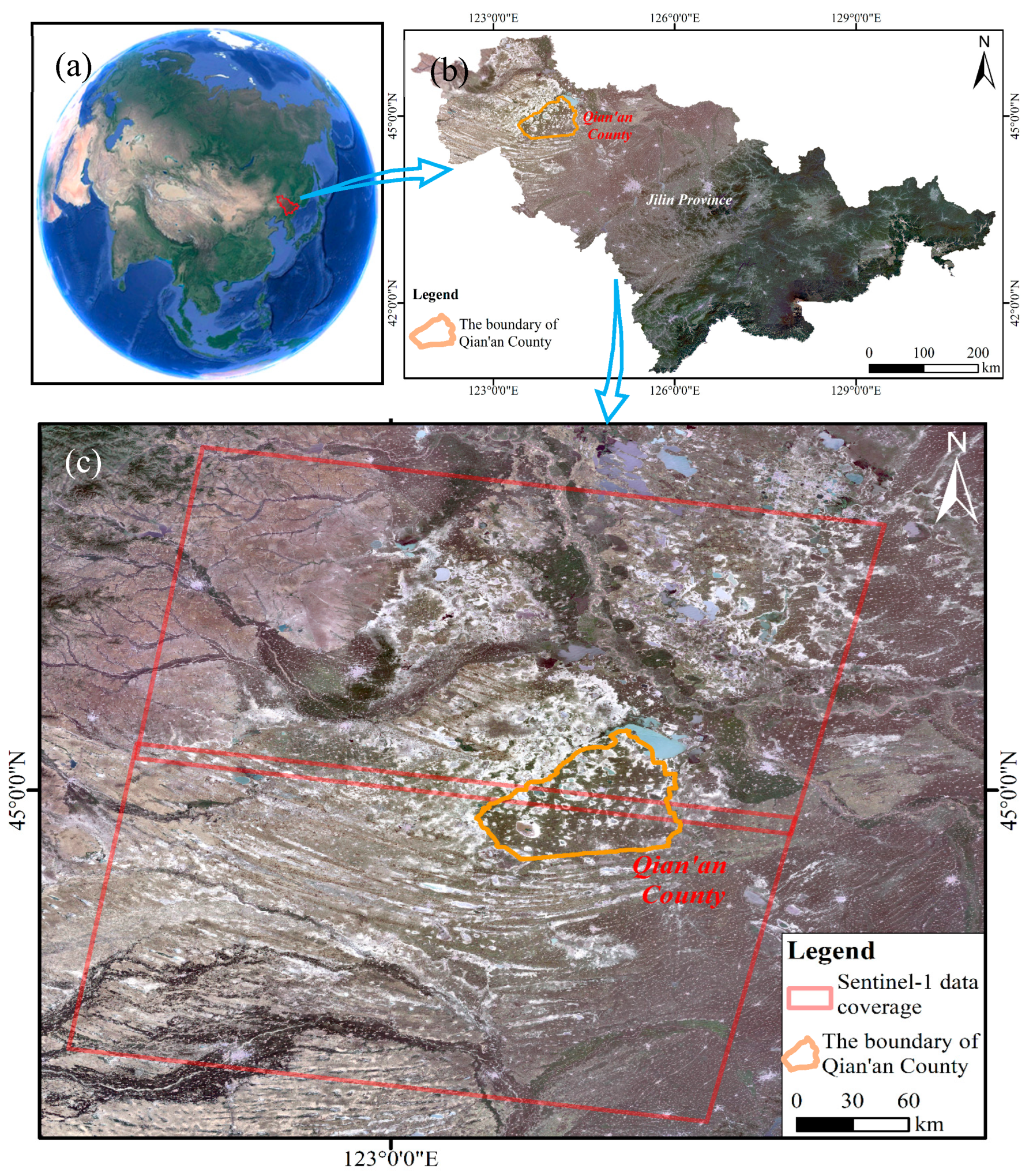
Figure 1. Location and data: (a,b) location of the study area; (c) coverage of Sentinel-1 data.
Remotesensing 16 03345 g001
Figure 2. Structure of multilayer perceptron.
Remotesensing 16 03345 g002
Figure 3. The deformation rate and profile position of the land subsidence in Zhouzi Village.
Remotesensing 16 03345 g003
Figure 4. Time series cumulative deformation of Zhouzi Village land subsidence.
Remotesensing 16 03345 g004
Figure 5. Temporal deformation characteristics of typical profiles (a) A-A′ coherent points deformation velocity; (b) B-B′ coherent points deformation velocity; (c) accumulated deformation of selected coherent points.
Remotesensing 16 03345 g005
Figure 6. Time series deformation prediction results based on three models.
Remotesensing 16 03345 g006
Figure 7. Distribution of land subsidence prediction errors. The blue points represent the minimum error, and the red points represent the maximum error.
Remotesensing 16 03345 g007
Figure 8. Deformation error of typical coherent point prediction.
Remotesensing 16 03345 g008
Table 1. Basic information of Sentinel-1 images.
SatelliteSentinel-1
Orbital directionDescending
Product typeSLC
Temporal coverage28 January 2017–18 December 2021
BandC band
Wavelength5.6 cm
Resolution5 × 20 m
Average incident angle36.02°, 36.94°
Polarization modeVV
Disclaimer/Publisher’s Note: The statements, opinions and data contained in all publications are solely those of the individual author(s) and contributor(s) and not of MDPI and/or the editor(s). MDPI and/or the editor(s) disclaim responsibility for any injury to people or property resulting from any ideas, methods, instructions or products referred to in the content.