Abstract
The technology for object detection in remote sensing images finds extensive applications in production and people’s lives, and improving the accuracy of image detection is a pressing need. With that goal, this paper proposes a range of improvements, rooted in the widely used YOLOv7 algorithm, after analyzing the requirements and difficulties in the detection of remote sensing images. Specifically, we strategically remove some standard convolution and pooling modules from the bottom of the network, adopting stride-free convolution to minimize the loss of information for small objects in the transmission. Simultaneously, we introduce a new, more efficient attention mechanism module for feature extraction, significantly enhancing the network’s semantic extraction capabilities. Furthermore, by adding multiple cross-layer connections in the network, we more effectively utilize the feature information of each layer in the backbone network, thereby enhancing the network’s overall feature extraction capability. During the training phase, we introduce an auxiliary network to intensify the training of the underlying network and adopt a new activation function and a more efficient loss function to ensure more effective gradient feedback, thereby elevating the network performance. In the experimental results, our improved network achieves impressive mAP scores of 91.2% and 80.8% on the DIOR and DOTA version 1.0 remote sensing datasets, respectively. These represent notable improvements of 4.5% and 7.0% over the original YOLOv7 network, significantly enhancing the efficiency of detecting small objects in particular.
1. Introduction
The technology for object detection in remote sensing images allows for precise and efficient identification of a specific object, determining the target’s specific category and pinpointing its location within the image. This technology finds important applications across diverse fields, including agricultural production, emergency rescue, geological exploration, and environmental monitoring. However, as they are obtained from high altitudes, remote sensing images often contain objects smaller than 32 × 32 pixels [1] and are set against complex backgrounds, and detecting objects from these images is challenging compared to other object detection tasks. Hence, exploring more accurate and efficient object detection algorithms is a hot research area and a goal of which we are in continuous pursuit [2,3,4,5,6,7,8,9,10].
Among the numerous object detection algorithms, the most popular today are based on neural networks [11]. These can be broadly divided into two categories: two- [12] and one-stage detection algorithms [13]. Compared to the former, one-stage detection algorithms excel due to their structural design, which eliminates the candidate box screening process, saving a lot of computational resources and resulting in higher efficiency. Within one-stage detection algorithms, the YOLO series of detection algorithms has continuously improved with version updates [14,15,16,17,18,19,20,21,22], achieving real-time output in inference speed and becoming the predominant algorithm in object detection [23]. Considering its accuracy and efficiency, we chose the popular new YOLOv7 algorithm for investigation [20,24,25,26,27].
When conducting thorough research on this algorithm [20], we discovered it has several shortcomings specific to remote sensing images. Firstly, the backbone network employs standard convolution or pooling operations to reduce the size of feature maps, which can lead to information loss during the layered transmission of remote sensing images containing numerous small objects. Secondly, the underlying feature layers of the network’s backbone are not fully utilized, and there is a lack of cross-layer connections within the network. Thirdly, the network lacks the introduction of attention mechanism modules. In order to attain greater accuracy and efficiency in object detection, inspired by the ELAN module structure in YOLOv7 and combining the ResNet [28] structure, we improved the network connections and attempted to introduce new convolution and attention mechanism modules to enhance the overall network performance. Through reasonable improvements to the original network, we achieved better object detection results on the DIOR [3] and DOTA version 1.0 [29] remote sensing datasets in comparison to the initial network.
We compared our improved network with other current mainstream algorithms on DIOR and DOTA version 1.0. The results showed that the improved network has a significant advantage in accuracy. The key contributions presented in this paper are as follows.
- Improved focus on small objects. Given that there may be numerous small objects in remote sensing imagery, we adopted a data augmentation strategy to increase the number of small objects. Simultaneously, we removed the standard convolution and pooling operations from the underlying YOLOv7 network, opting for stride-free convolution to minimize information loss concerning small objects, which often occurs during feature extraction. This enhancement significantly boosts the network’s attention to and detection accuracy of small objects.
- Deep utilization of feature layers. To elevate the network’s overall semantic expression capability, we integrated multiple attention mechanism modules and introduced cross-layer connections between different levels of the network. These advancements not only refine the network architecture but also enable more efficient utilization and fusion of information from various feature layers, thereby enhancing the abilities of the network to extract features and express semantic information.
- Facilitating comprehensive network weight updates. We employed more efficient activation and loss functions to ensure more effective gradient information backpropagation and network weight updates during training. Additionally, we introduced an auxiliary network at the network’s base for intensified training, further propelling the entire network toward an ideal target model. These measures collectively promote comprehensive and in-depth network weight updates, elevating the network performance.
The remainder of this paper is organized into seven key parts. Section 2 presents work related to the article’s content. Section 3 details the specific improvement, relevant details, and principles of the improved algorithm. Section 4 outlines the experimental configuration, utilized datasets, and training processes. Section 5 presents and analyzes the outcomes of the experiments. Section 6 delves into some of the outcomes and phenomena observed in the experiments. Finally, in the last chapter, we summarize the article and propose future research prospects. For ease of reading, we have compiled some important abbreviations of terms in Table 1.

Table 1.
Nomenclature.
2. Relevant Research
This section presents the evolution of object detection, elaborates on the methodologies employed in network improvement, and compares our work with closely related studies.
The evolution of algorithms for object detection comprises two separate eras. Initially, there was a period of manually designing feature extraction algorithms. During this time, researchers analyzed features specific to different targets and devised tailored feature extractors. These algorithms were characterized by their simplicity but lacked adaptability, often requiring a fresh analysis of features and the creation of new algorithms for distinct targets [30,31]. However, with the advent of neural networks, particularly deep neural networks, object detection shifted towards complex algorithms with stronger adaptability [32,33,34,35]. These networks automatically learn and update their feature extraction parameters for various targets, eliminating the need for laborious manual feature extractor design.
The application of neural network algorithms in object recognition evolved from image classification tasks. Subsequently, two-stage algorithms emerged, such as RCNN [32] and SSD [36]. However, since these lacked computational speed, faster one-stage algorithms like YOLO appeared [14]. Initially, the one-stage methods lagged in detection accuracy compared to two-stage methods, but both have since evolved and improved. The advent of transformer [37] further propelled object detection algorithms towards attention mechanisms, exemplified by models like deformable DETR [38]. However, while these networks offer decent detection results, they are bulky and challenging to train, in contrast to the one- and two-stage methods.
In remote sensing image analysis, object detection algorithms face heightened demands due to complex backgrounds, varied target sizes, and uneven distributions of targets. Two-stage detection algorithms excel in handling complex backgrounds and multi-scale targets with high accuracy, but may be limited in their capacity to achieve a real-time processing speed for remote sensing images. Conversely, one-stage detection algorithms offer faster detection while maintaining acceptable accuracy, making them more suitable for real-time remote sensing tasks. Considering both accuracy and speed, YOLOv7, a one-stage detection algorithm, was selected for this study. YOLOv7 builds upon the rapid detection capabilities of the YOLO series and demonstrates enhanced accuracy and robustness through optimizations, enabling it to perform well in remote sensing image analysis.
We chose the commonly applied YOLOv7 as our foundation. We found that the accuracy of detecting small targets and complex backgrounds in this network needs to be improved. The performance of modules in the network needs to be improved, and the fusion of information in the network framework is not sufficient. After analyzing the features and attributes of remote sensing imagery and identifying shortcomings in the original network, inspired by various research outcomes, we improved the original YOLOv7 network. We replaced some of the bottom layers’ standard convolutions and pooling operations with the stride-free convolution (SFC) module [39]. This module enables feature maps to scale with minimal information loss and increases the number of feature layer channels. Additionally, we incorporated two attention mechanisms—the convolutional triplet attention (CTA module) [40] and contextual transformer (CoT) module [41]—within the initial network framework to improve its capability in extracting target feature information. Both attention mechanisms fuse information within feature maps in novel ways, enriching the network’s semantic representation of the image content.
Regarding network connectivity, we adopted the skip connection approach from ResNet to directly integrate low-layer feature maps into the network’s feature fusion network, enhancing the utilization of small object information. To facilitate gradient information propagation during backpropagation and accelerate network convergence, we employed the more efficient Mish [42] activation function and introduced an auxiliary network to reinforce gradient conduction in YOLOv7’s lower layers during training. For a more precise measurement of the network’s approximation of the model, we opted for MPDIoU loss [43], which has demonstrated impressive performance in various experiments, ensuring that the network’s training results more closely align with the ideal model.
Considerable exploration has occurred in the field of object detection using remote sensing images, among which the improvement of using YOLO network mainly includes the transformation of network structure, optimization of loss function, etc. We integrate multiple advantages, so our approach stands out by building upon the efficient YOLOv7 network structure [3,44,45,46]. We carefully analyzed the characteristics of both the network and detection objects, combining the strengths of various methods to enhance the overall model. While there are many modifications targeting skip connections in YOLO series models [47,48], our distinction lies in connecting low-layer feature information to the feature fusion network, so the network’s proficiency in extracting and semantically representing small objects is improved. By combining more efficient activation functions, loss functions, and auxiliary networks, we facilitate gradient information backpropagation in multiple ways, allowing our improved network’s training results to more closely approximate the ideal ones. This sets us apart from other YOLO-based enhancement studies [49,50,51,52,53].
3. Methodology
Herein, we first introduce the detailed network structural modifications and the modules employed in these adjustments. Subsequently, we elaborate on the loss functions used in this model and the methods employed for model evaluation.
3.1. Network Modifications
Considering the characteristics of object detection assignments in remote sensing imagery, where small objects predominate and the backgrounds are often complex, we conducted a comprehensive examination of the YOLOv7 network. Targeting its shortcomings, we made several improvements. Figure 1 depicts the initial framework of YOLOv7, and Figure 2 shows our modifications to YOLOv7.
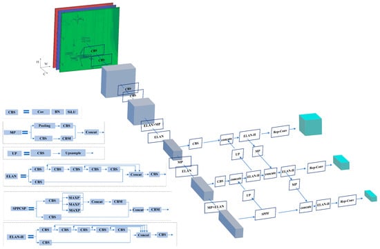
Figure 1.
Original network.
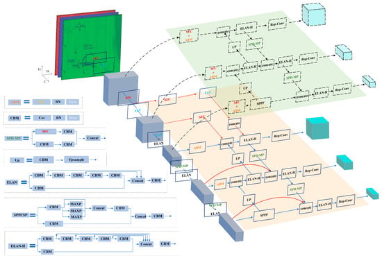
Figure 2.
Modified network structure.
Figure 1 illustrates the YOLOv7 network architecture. In Figure 1, the cubes represent the input or output feature maps. The feature map dimensions are denoted by the coordinates, with W referring to the width, H the height, and C the channel count. The abbreviations in dark-blue rectangles depict the corresponding network modules, while the blue lines or arrows show the flow of information. A detailed explanation of the internal structure of each network module can be found in the diagram’s bottom-left section.
The refined network structure is exhibited in Figure 2, with the modified parts highlighted in different colors. In terms of network connectivity, the red curves indicate newly added skip connections in contrast to the initial structure. In the diagram’s upper-right corner, the dashed line represents an auxiliary network used during training. Modules that have been modified compared to the original network are highlighted in different colors. Parts that retain the same color as in Figure 1 indicate that the network structure and content remain unchanged.
When comparing Figure 1 and Figure 2, it can be seen that our network modifications mainly concern three aspects. Firstly, more connections have been added, so more feature maps can be input for feature fusion. Specifically, feature maps produced at lower layers are connected to the feature fusion part, enhancing the capacity of the network to extract feature information from smaller items. Secondly, different network modules are employed. In the improved network, we have replaced standard convolution or pooling modules with stride-free convolutions and various attention mechanism modules, enhancing the ability of the network to extract features. Thirdly, an auxiliary network has been introduced, and the activation function has also been changed. This aims to strengthen the backpropagation of gradient information to the lower layers during training, addressing the issue of slow and weaker weight updates in the lower layers caused by the deep network structure. Our upgrade helps the model learn target features better during training, especially improving its recognition ability in complex scenes.
3.2. Modules Used in This Network
3.2.1. Stride-Free Convolution Module
In Figure 3, W is the width, H the height, and C the channel count of the feature map. The blue arrows indicate the flow of information, and the left- and rightmost sides of the figure depict the input and output feature maps, respectively. “Decom” in the figure represents the pixel-wise segmentation of the feature map, resulting in maps with half the original height and width. “Concate” signifies the joining of these sub-feature maps in the channel dimension, followed by a convolution operation using a 1 × 1 kernel to generate the output from the concatenated feature map.
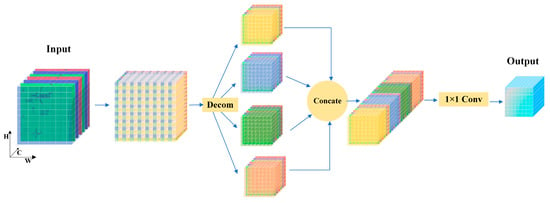
Figure 3.
Stride-free convolution module.
Equation (1) provides the mathematical formula corresponding to Figure 3:
In Equation (1), represents a 1 × 1 convolution operation; and denote the input and output feature maps, respectively, and , , , and represent the decomposed sub-feature maps. and denote the feature map’s width and length, respectively. The meaning of the formula is shown in Figure 3, where [0: L-1:2, 0: W-1:2] is expressed as a pixel-wise decomposition of each channel in the length and width directions, corresponding to the “Decom” operation in Figure 3. The notation indicates sampling every other pixel value from 0 to along the length direction and similarly for the width direction.
In Figure 3 and Equation (1), we can observe that the stride-free convolution module segments the feature map by pixels and then concatenates the segmented feature maps along the channel direction. This module is mainly applied to the bottom layer of the backbone network of the network. This operation avoids any loss of detailed information from the image during the pooling process while expanding the number of channels in the input network. Therefore, compared with ordinary convolution or pooling operations, this method preserves more detailed information when scaling down the image and avoids losing information about small objects due to their smaller scale in this operation. At the same time, the length of the generated feature map increases in the channel direction, which enriches the small object information contained in the feature map and has a positive effect on the network, especially for the extraction of small object features.
3.2.2. Convolutional Triplet Attention Module
In Figure 4, the cubes represent the network’s input or output feature maps. The letters C, H, and W marked alongside the arrows denote the directions of the feature maps’ channels, height, and width, respectively. The rotating arrows on the H or W axis represent a 90-degree rotation. “Conv” denotes a convolution operation, and “Mish” represents activation. The blue lines with arrows in the figure indicate the information’s flow within the network. Equation (2) illustrates the contents of Figure 4:
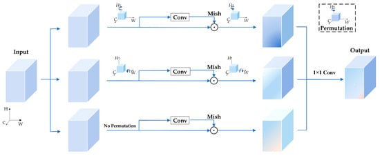
Figure 4.
Convolutional triplet attention module.
In Equation (2), denotes the input feature map, while signifies the corresponding output feature map. , , and denote the intermediate feature maps generated within the network. or represents a 90-degree rotation of the feature map along the H or W axis. denotes a standard 3 × 3 convolution, represents an activation function, and indicates a 1 × 1 convolution.
When combining Equation (2) and Figure 4, we can observe that the convolutional triplet attention module combines convolutions from multiple angles. Compared with standard convolutions, the feature maps generated by it contain more feature information, which enables the network to fully utilize the existing information and enhance its ability to obtain feature information.
3.2.3. Contextual Transformer Module
In Figure 5, “key” is obtained through a 3 × 3 convolution and “weight” is derived by applying a 1 × 1 convolution to the combination of “key” and “query.” “Value” and “weight” are multiplied element-wise to produce a dynamic result, which is then added to “key” to generate the final output. The network module depicted in Figure 5 can be mathematically represented using Equation (3):
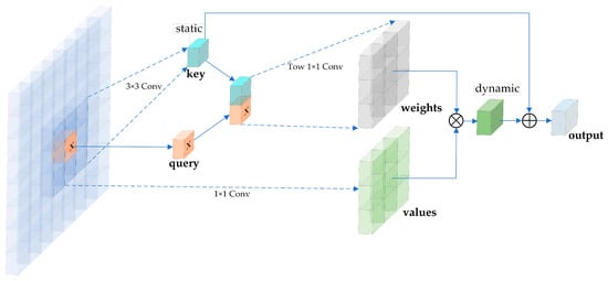
Figure 5.
Schematic diagram of the contextual transformer module.
In Figure 5, “query,” “key,” and “values,” respectively, represent vectors that correspond to , , and in Equation (3). Additionally, and in Equation (3) correspond to the 1 × 1 and 3 × 3 convolutions in Figure 5, respectively. In Equation (3), represents the “query” vector, is the feature map surrounding the “query” vector, and is the input feature map. and represent the “values” and “key” vectors generated corresponding to the “query” vector, respectively. and indicate 1 × 1 and 3 × 3 convolutions, respectively. represents the attention heads’ number, denotes the linear transformation weights, and represents the value space of .
When combining Figure 5 and Equation (3), it becomes apparent that the generation of the key relies on the values surrounding the query, and the key is once again integrated into the final result. We introduce an attention mechanism to enhance the model’s perception of complex backgrounds and multiple small targets. This mechanism helps the model concentrate on important areas and allows the attention mechanism to incorporate local contextual information, supporting the network to capture object features. The addition of this attention mechanism changes the deficiency in ordinary convolution that only extracts features without being able to determine the importance of the features based on them. When facing scenes with complex background information, the network can more effectively filter out useless background information and focus on extracting target features.
3.3. Loss Functions and Performance Measures
3.3.1. Loss Functions Used in the Model
IoU’s interpretation is visually demonstrated in Figure 6. On the left, the red rectangle means the predicted bounding box, while the green rectangle denotes the labeled bounding box. The mathematical expression for IoU is shown in the right half of the figure.
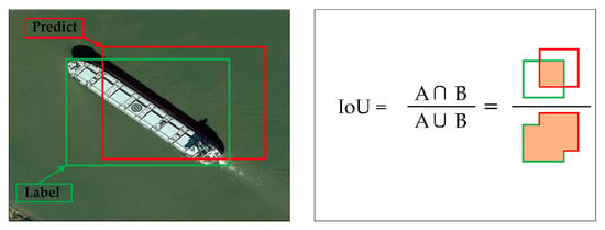
Figure 6.
Visual representation of IoU.
MPDIoU’s notion is visually explained through Figure 7. The letters on the left are explained on the right. The mathematical representation can be found in Equation (4):
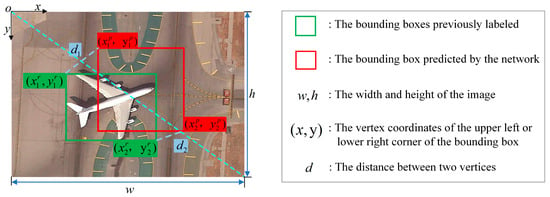
Figure 7.
A visual representation of MPDIoU.
In Equation (4), L_M represents the MPDIoU loss, and the meanings of the other letters are consistent with those in Figure 7.
3.3.2. Overall Loss Function
The numerical values’ meaning at every position in the network’s overall output results is explained in Figure 8. The number 5 represents the five values in the output results, which are x, y, w, h, and c. The number 20 represents the probability figures associated with 20 mixed object classifications. This result is consistent with the network’s labels, facilitating the calculation of the network’s overall loss.
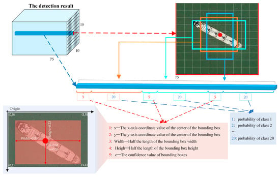
Figure 8.
Network’s output results.
The total loss function is presented in Equation (5):
In Equation (5), the network’s overall loss is represented by , which primarily comprises three elements: the loss of a category is represented by , the loss of confidence is labeled , and the loss of a bounding box is denoted . is the cross-entropy loss between the true probabilities and predicted probabilities for each category. represents the true confidence value, while represents the predicted confidence value. is the overall count of grids into which the image is divided. denotes the -th grid in , and denotes the -th anchor box within the -th grid, where can take a value of 1, 2, or 3. indicates that there is a real target object within the -th predicted anchor box corresponding to the -th grid, while indicates the opposite. , , , and are the weight coefficients for various losses, with values of 0.2, 0.1, 0.05, and 0.15, respectively.
3.3.3. Evaluation
Here we introduce some concepts and calculation methods.
In Equations (6) and (7), the meanings of and are consistent with those expressed in Figure 9, along with their calculation methods. represents the integral value of the region between the P–R curve and the coordinate axes, and its specific calculation method is given by Equation (6). represents the mean of AP values across categories, and its specific calculation method is provided by Equation (7).

Figure 9.
Schematic diagram of precision and recall calculation formulas.
4. Datasets and Experimental Setup
Herein, firstly, the remote sensing datasets used in our experiments and data preprocessing steps are introduced. Then, we detail the experimental setup. Finally, we outline the overall training process.
4.1. Datasets Used for Training
DIOR Dataset [3] is an optical remote sensing imagery dataset. The dataset comprises 23,463 images, encompassing 190,288 instances distributed across 20 distinct object categories: train station, dam, golf field, stadium, ground track field, basketball court, airport, chimney, overpass, bridge, windmill, expressway service area, harbor, baseball field, airplane, tennis court, storage tank, expressway toll station, vehicle, and ship. This dataset is characterized by significant variations in object scales, diverse background environments, high inter-class similarity, and intra-class diversity. All images in this dataset are consistently sized at 800 × 800 pixels. We split this dataset into three sets, training, validation, and test, containing 14,077, 4694, and 4692 images, respectively.
DOTA version 1.0 Dataset [29] is another optical remote sensing imagery dataset comprising 2806 images with 188,282 instances across 15 categories: ground track field, basketball court, swimming pool, roundabout, soccer ball field, baseball diamond, storage tank, helicopter, bridge, tennis court, harbor, plane, large vehicle, small vehicle, and ship. This dataset features images from diverse sources and scenes. The image sizes vary, with the largest dimensions reaching 4000 × 4000 pixels. Therefore, during experiments, we cropped the images to a uniform size of 1024 × 1024 pixels with a 20% overlap, filling any empty spaces with a black background. The dataset is divided into a training set with 15,749 images, a validation set with 5297 images, and a test set containing 5296 images.
4.2. Data Processing
To enhance the training effectiveness and optimize the model’s performance during training, we applied image augmentation techniques to the training dataset. Data augmentation is one of the key factors in the final performance of a model. We integrate multiple data augmentation techniques to simulate more complex background environments and smaller targets, and integrate them into the existing dataset. The ordinary image transformation is used to simulate the complexity of the background and target state, while the Mosaic operation is used to transform the size of the target to generate more small targets. Figure 10 illustrates the augmentation methods.
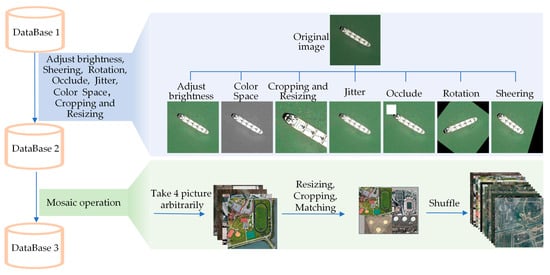
Figure 10.
Data augmentation methods.
In Figure 10, “database 1” on the right side represents the original dataset, while “dataset 3” denotes the dataset used for training. The texts alongside the blue lines indicate the corresponding operations performed on the data. When transitioning from database 1 to database 2, we primarily applied seven operations to the images, namely, adjust brightness, shearing, rotation, occlusion, jitter, color space, and cropping and resizing manipulation. The effects of these operations on the images are illustrated in the upper part of Figure 10. When moving from database 2 to database 3, we primarily employed the Mosaic operation [54], which involves randomly selecting four images from the dataset, randomly resizing and cropping them, and then stitching together a new one. The processed images are then mixed back with the original images, as depicted in the lower part of Figure 10.
4.3. Environment and Settings
Our model was implemented using the Python language within the PyTorch (torch 2.2.2+cu121) framework on an Ubuntu 22.04 operating system. Our hardware environment consisted of a Xeon(R) W-3495X CPU (Santa Clara, CA, USA), an NVIDIA RTX 6000 Ada GPU (Santa Clara, CA, USA), and 64 GB of RAM. Table 2 lists some of the parameter settings.

Table 2.
Model training parameters.
The input images were uniformly resized to 640 × 640 pixels. Due to hardware limitations, the duration of the training epochs was arranged to be 180, and the training batch size was established as 32. As for the optimizer, an Adam optimizer [55] was chosen, and we employed a momentum of 0.937, a learning rate set at 0.01, and a weight decay factor of 0.0005 in our approach.
4.4. Model Training
In Figure 11, we illustrate the modified network training process. The text within the blue boxes provides descriptions of the main training operations, and the blue arrows indicate the sequential order of these operations. Throughout the entire training process, we adopted the concept of transfer learning. The model was initially trained on the MS COCO dataset [56] as a preparatory step. Subsequently, the network leveraged the pre-trained weights from the target dataset to acquire the ultimate model weights.
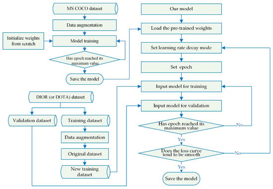
Figure 11.
Flowchart of model training.
5. Results and Analysis
5.1. Label Statistics for Training Sets
We conducted statistical analyses on the labeled data from the augmented DIOR and DOTA version 1.0 training sets, considering different categories and the proportion of bounding box sizes. Figure 12 shows the results.
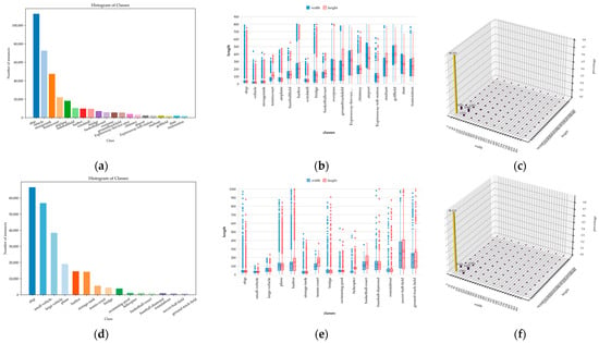
Figure 12.
Label statistics for the training sets. (a,d) Instance count for each category in the augmented DIOR and DOTA version 1.0 training sets, respectively. Different colors represent different categories, and the height of each bar signifies the total count of instances. (b,e) Box plots representing the length and width distributions of instances for every category. The blue box plots represent the width distribution, while the red box plots represent the length distribution. Outliers are indicated by circles outside the box plots, and the category order is consistent with (a) or (d). (c,f) Histograms of the length and width distributions for all instances in the DIOR and DOTA version 1.0 training sets, respectively. The height of each bar represents the proportion of instances within a specific size range relative to the overall instance count in the dataset.
In the DIOR and DOTA version 1.0 datasets, all images have three channels, and some distribution information is shown in Figure 12. In Figure 12a,d, it is evident that the instance count differs among various categories within the training datasets. Figure 12b,e reveal that the distribution of the bounding box sizes differs among categories, with the three most frequent categories having bounding box sizes below 100 × 100. Upon closer examination of Figure 12b,e, we can observe that over 80% of the targets in both datasets have sizes below 64 × 64. Based on Figure 12, we can conclude that the targets are generally small in both datasets, which is a distinctive feature of remote sensing images.
5.2. Presentation of Detection Results from the Improved Model
To provide an intuitive account of detection effectiveness, in Figure 13 and Figure 14, we exhibit the detection outcomes achieved by the improved model.
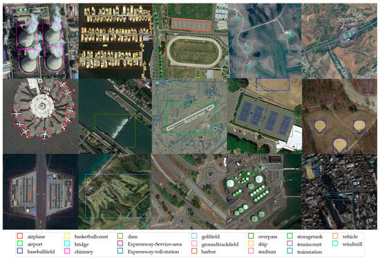
Figure 13.
Detection results on the DIOR dataset.
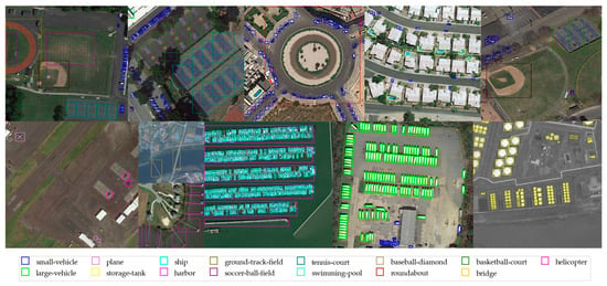
Figure 14.
Detection results on the DOTA version 1.0 dataset.
In Figure 13 and Figure 14, the rectangular boxes represent objects detected in the images. Different-colored rectangular boxes indicate different categories detected by the model. The correspondence between the colors of the rectangular boxes and the detected categories is explained in the legend below each figure.
5.3. Comparison before and after Model Improvement
To assess the efficacy of model enhancements, we performed a comparative analysis. In Figure 15, we offer a comparison between mAP50 and mAP50:95 throughout the training process. Additionally, Figure 16 illustrates precision–recall (PR) curves for different categories of targets in each dataset, comparing the models before and after improvement.
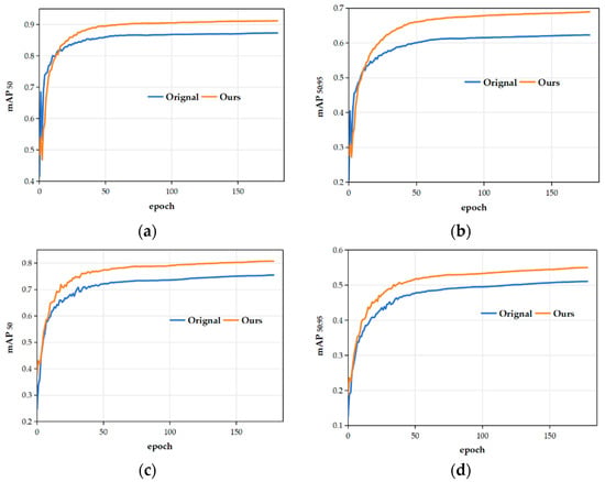
Figure 15.
Comparison of mAP during the training process of the improved model on various datasets. In each sub-figure, the training epochs’ sequence is displayed along the horizontal axis, while the vertical axis displays the corresponding mAP50 or mAP50:95 metrics. The yellow curve represents the improved model, while the unimproved model’s performance is depicted by the blue curve. (a,b) mAP50 and mAP50:95 curves of the models before and after improvement on the DIOR dataset. (c,d) mAP50 and mAP50:95 curves of the models before and after improvement on the DOTA version 1.0 dataset.
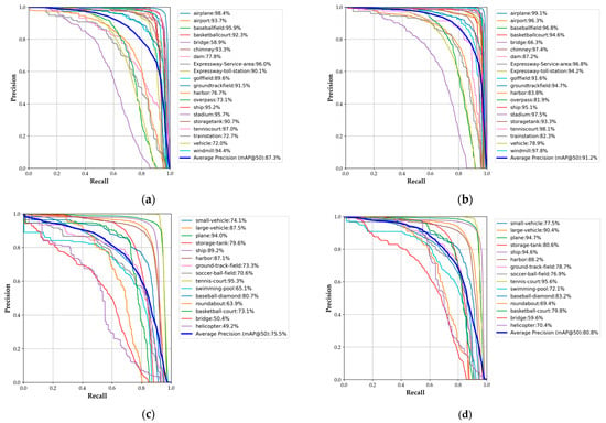
Figure 16.
Precision–recall (PR) curves for different categories of objects in various datasets using the improved model. In each sub-figure, the recall value is plotted on the x-axis, whereas the precision value is shown on the y-axis. Different-colored curves correspond to different categories of objects, where the blue curve indicates the average AP across all categories. The numerical value following each category name in the legend represents the AP50 for that particular category. (a,b) PR curves for the models before and after improvement on the DIOR dataset, respectively. (c,d) PR curves for the models before and after improvement on the DOTA version 1.0 dataset, respectively.
In Figure 15, one can note that for the DIOR dataset, the differences begin to emerge at around the 20th epoch, and the gap gradually widens thereafter. For the DOTA version 1.0 dataset, the differences start to appear at around the 15th epoch, with a progressively increasing disparity. At the 50th epoch, the mAP50 and mAP50:95 curves for both models tend to flatten, indicating a slowing growth. When comparing the blue and yellow curves, it can be surmised that the improved model exhibits better performance than the original model.
Figure 16 makes it apparent that the refined model boosts the detection outcomes for various object categories on both datasets. However, there are significant variations in the detection outcomes for different categories. For more detail, we compiled Table 3, Table 4, Table 5 and Table 6, which summarize the AP50 values for each category and the corresponding numbers for the object category names in the DIOR and DOTA version 1.0 datasets. The letter R or A before each number represents the last letter of the dataset name, and below each number in Table 3 and Table 4, the specific name of the corresponding object category is provided.

Table 3.
Correspondence table for object category names and their numbers in the DIOR dataset.

Table 4.
Correspondence table for object category names and their numbers in the DOTA version 1.0 dataset.

Table 5.
AP50 (%) of each category for DIOR.

Table 6.
AP50 (%) of each category for DOTA version 1.0.
Table 5 and Table 6 present the specific values of AP50 (%) for every category in the DIOR and DOTA version 1.0 datasets, respectively, for the models before and after improvement. For an intuitive comparison, we have visualized the values in Table 5 and Table 6 using radar charts in Figure 17.
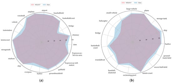
Figure 17.
Comparison of AP50 for various categories. (a) Comparison of AP50 for various categories on DIOR; (b) comparison of AP50 for various categories on DOTA version 1.0.
Table 7 presents the results of our significance analysis of the data in Table 5 and Table 6. In Table 7, we can observe significant differences in the average performance between YOLOv7 and our improved model on the DIOR dataset (t-statistic = −5.629211, p-value = 0.000020). This indicates that the null hypothesis—that there is no difference in performance—can be rejected, with us accepting the alternative hypothesis that there is a significant difference in performance between the two models. Similar trends were observed on the DOTA version 1.0 dataset (t-statistic = −3.929775, p-value = 0.001511), where the p-value was slightly higher than the conventional significance level, but still signified significant differences, especially given the large dataset. Taken together, these findings consistently demonstrate that our model exhibits superior performance to that of YOLOv7 in object detection tasks. The difference is attributed not to random error, but to genuine disparities in model performance.

From Figure 17a, we can observe that for the DIOR dataset, the improved model shows increase in AP50 for the categories of train station, bridge, dam, overpass, vehicle, and harbor, with improvements of 13.2%, 12.5%, 12.1%, 12.0%, 9.6%, and 9.3%, respectively. In Figure 17b, on DOTA version 1.0, the improved model demonstrates notable gains in AP50 for the categories of helicopter, bridge, swimming pool, and basketball court, with increases of 43.0%, 18.2%, 10.8%, and 9.2%, respectively. These improvements indicate that the ability to extract object features and detection capabilities across different categories have been bolstered. Figure 12e then makes it apparent that the objects in the categories of helicopter, bridge, and swimming pool are predominantly sized 100 × 100 pixels or less, suggesting that the improved model boosts small object detection. For further analyses, we present confusion matrices in Figure 18.
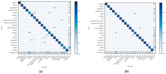
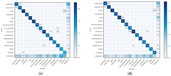
Figure 18.
(a,b) Confusion matrices for the models before and after improvement on DIOR. (c,d) Confusion matrices for the models before and after improvement on DOTA version 1.0.
In this figure, the values within the grids indicate the probability of a particular category (on the vertical axis) being identified as another category (on the horizontal axis), and the color intensity of the grids increases with higher numerical values. Evidently, the refined model has boosted detection precision in all categories, as can be seen when comparing (a) with (b) or (c) with (d) in Figure 18. There is a reduction in misidentification among different categories, and the proportion of missed detections for objects in the background has decreased for various categories.
For an intuitive demonstration, we present a comparison of the detection results in Figure 19 and Figure 20. In Figure 19, the solid-line boxes of various colors represent different detected objects, and the corresponding target names are explained in the legend. The dashed box outlines the selected area for comparison. The first column shows the pre-improvement model’s detection results. In the third column, we can see the detection results obtained by the refined model, and the second column provides enlarged views of the selected comparison areas.
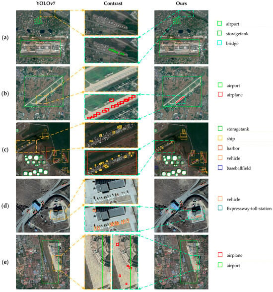
Figure 19.
Comparison of the detection results on DIOR. (a–e) Local area comparisons of the model detection results in five different scenarios.
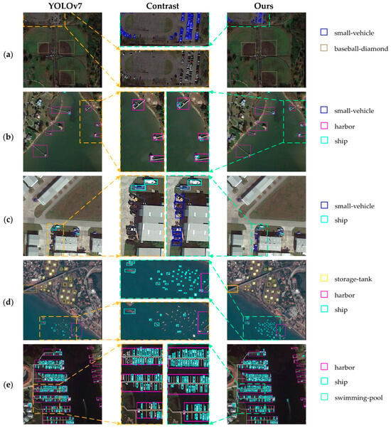
Figure 20.
Comparison of the detection results on DOTA version 1.0. (a–e) Local area comparisons of the model detection results in five different scenarios.
Upon comparing the selected and enlarged comparison areas in Figure 19, we can observe the following. Compared to the pre-improvement model, more storage tanks are detected in Figure 19a, the airplane is correctly detected in Figure 19b, a higher number of ships are detected in Figure 19c, more small vehicles are detected in Figure 19d, and a small airplane is also detected in Figure 19e. Clearly, the improved model demonstrates stronger detection capabilities for small objects.
Similarly, comparing the selected and enlarged comparison areas in Figure 20 reveals the following. Compared to the pre-improvement model, a missed small vehicle is successfully detected in Figure 20a, some concealed ships are detected in Figure 20b, a larger number of small vehicles are detected in Figure 20c, more small ships are detected in Figure 20d, and ship detection is more precise in Figure 20e. Thus, we may conclude that the improved model represents a significant advancement in small object detection.
5.4. Ablation Experiments
To delve deeper into the functions of diverse modules within the improved model, ablation experiments were performed on each individual module incorporated into the improved model, and the results are given in Table 8. For convenience, the module names are abbreviated, where “baseline” represents the original network, “SFC” stands for the stride-free convolution module, “CTA” denotes the convolutional triplet attention module, “CoT” signifies the contextual transformer module, “MPD” refers to the MPDIoU loss, “SKC” represents the added skip connection in the network, and “AUN” indicates the auxiliary network.

Table 8.
Ablation experiments on two datasets.
In Table 8, when reviewing the values in the second-last column of the table, we can find that the use of skip connections, the SFC module, and the auxiliary network significantly enhances the network’s performance. Specifically, skip connections integrate more feature layers into the network, the SFC module reduces the loss of information pertaining to small targets during the initial stages, and the addition of an auxiliary network facilitates the updating of bottom weights during training. These findings align with the overall improvement in the network’s performance, particularly its enhanced ability to detect small objects. Furthermore, the incorporation of attention mechanisms introduces contextual information and a broader receptive field into the feature maps, positively impacting the detection results for objects of other sizes.
Table 9 shows the ablation experimental data of a single module added to the network. When comparing each row of data in Table 9 with the previous one, it can be observed that the added modules all contribute positively to the network’s performance. Among them, SFC, SKC, and AUN modules have the most outstanding contributions to the network, consistent with the results in Table 8.

Table 9.
Ablation experiments on two datasets.
5.5. Comparative Experiments
We compared our model to the widely used models on both the DIOR and DOTA version 1.0 datasets, and Table 10, Table 11, Table 12 and Table 13 showcase the outcomes.

Table 10.
Comparative experiments on DIOR.

Table 11.
AP50 (%) comparative experiments for each category on DIOR with various modules.

Table 12.
Comparison experiments on DOTA version 1.0.

Table 13.
AP50 (%) comparison experiments for each category on DOTA version 1.0 with various modules.
Table 10 shows the training results on DIOR. When comparing the results of different models, in terms of computational complexity, due to the addition of some modules in the improved model, the number of parameters has increased slightly compared to before, resulting in a slight increase in computational complexity. This has caused the reference speed of the modified network to be slightly lower than that of the original network, but due to the small increase, it is still within the acceptable range for real-time detection. Comparing the mAP values, it can be seen that the improved model has superior detection performance compared to the latest YOLOv8 and YOLOv9 models. To provide more detailed data, we present the AP50 values for every category in Table 11 and the corresponding PR curves in Figure 21.
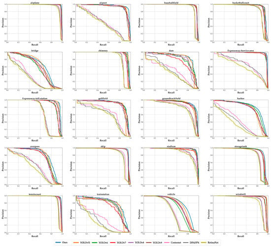
Figure 21.
Precision–recall curves for each category on DIOR.
To simplify data presentation, the first line in Table 11 lists the object numbers for each category in the DIOR dataset, and Table 3 contains the exhaustive category names.
Figure 21 presents PR curves corresponding to the data in Table 11, where different colors of curves depict the detection results from various models, and the specific model name corresponding to each colored curve is indicated in the legend at the bottom of the figure. The PR curve for each category of objects from left to right in the figure corresponds to the data in each column of Table 11.
When combining Table 11 and Figure 21, evidently, our improved model has advantages over other models in detecting objects in the three categories of airplane, harbor, and vehicle. Referring to Figure 12b, we can characterize airplane and vehicle objects as being smaller than 100 × 100 and relatively concentrated, while harbor targets have a wide range of sizes and many outliers. From these results, it can be surmised that our network demonstrates superiority in detecting small objects and extracting features from objects at different scales.
Table 12 showcases the training outcomes of various models on DOTA version 1.0. When comparing the detection outcomes across various models, our model demonstrates advantages over the latest YOLOv8 and YOLOv9 models while maintaining a comparable inference speed to the original network. Similarly, for more details, we showcase the AP50 values for every category in Table 13 and the corresponding PR curves in Figure 22.
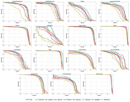
Figure 22.
Precision–recall curve for each category on DOTA version 1.0.
The first line of Table 13 lists the target numbers, aligning with the numbering in Table 4, where the specific category names are detailed. The PR curves corresponding to the data in Table 13 are exhibited in Figure 22. In this figure, curves of different colors depict the detection outcomes of diverse models, and at the bottom of Figure 22, the legend specifies the model names corresponding to each colored curve. The PR curves for each object category, from left to right, correspond to the data presented in each column of Table 13.
When combining Table 13 with Figure 22, it becomes evident that our improved model has an edge over other models in detecting objects within seven categories: ground track field, helicopter, bridge, ship, small vehicle, soccer ball field, and swimming pool. When referring to Figure 12e, it is noteworthy that targets such as the bridge, ship, small vehicle, swimming pool, and helicopter are typically smaller than 100 × 100 and that the distributions of their length and width are relatively concentrated, whereas the ground track field and soccer ball field objects exhibit a wide range of sizes and there are numerous outliers in their distributions. This further illustrates the strengths of our network in detecting small objects and extracting features from different-sized objects.
The detection results of different models across various datasets are visualized in Figure 23 and Figure 24. In both figures, the title above each image denotes the model used for detection, and the corresponding detection outcomes are displayed beneath the title. The first image represents the original image to be detected. Detected objects are indicated by colored rectangular boxes, and the key below each image clarifies the object names corresponding to each color.
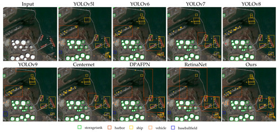
Figure 23.
Comparison of detection outcomes among various models on DIOR.
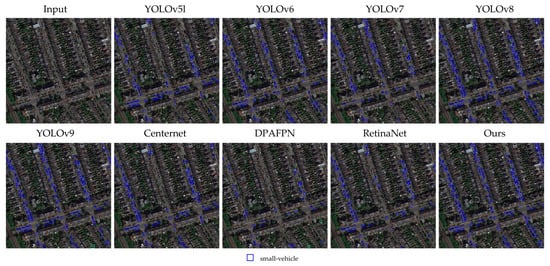
Figure 24.
Comparison of detection outcomes among various models on DOTA version 1.0.
Based on the results presented in Figure 23, when specifically focusing on the ship and vehicle categories, our model detects the highest number of these objects. Meanwhile, the other models exhibit varying degrees of missed detections for these two categories.
When examining the detection outcomes in Figure 24, particularly for the small vehicle category, it can be surmised that our model detects the highest number of these targets, while the other models show different degrees of missed detections. Combining the insights from Figure 23 and Figure 24 reveals that our model has higher precision in detecting small objects.
5.6. Heatmaps
To further explore the differences between the original and improved models, we employed GradCAM [60] technology to generate the heatmaps shown in Figure 25 and Figure 26. In both Figure 25 and Figure 26, the leftmost column displays the original input images, while the middle and right columns exhibit the heatmaps generated using GradCAM during the inference process for the models before and after improvement, respectively. In the heatmaps, the red highlighted areas indicate the regions where the model focuses. As the red color of a region intensifies, the model’s attention to that specific area increases.
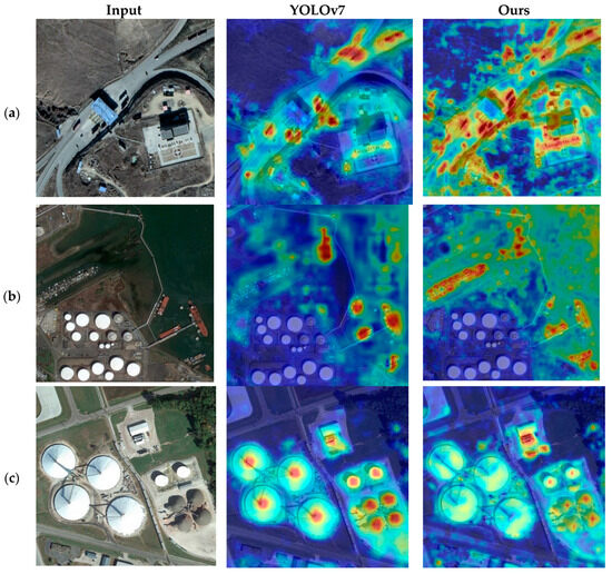
Figure 25.
Heatmaps generated by GradCAM on DIOR. Images (a–c) correspond to three different scenes from the DIOR validation set.
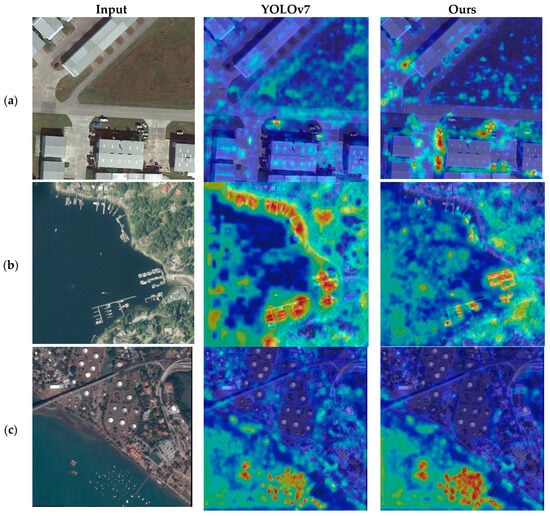
Figure 26.
Heatmaps generated by GradCAM on DOTA version 1.0. Images (a–c) correspond to three distinct scenes from the DOTA version 1.0 validation set.
Comparing the last two columns in Figure 25 reveals that our model focuses more on smaller objects. Specifically, in Figure 25a, it can be seen that the model produces more highlighted areas, covering a broader range of small objects. Similarly, in Figure 25b, on the left side, more ships are covered by the red highlighted areas. On the right side of Figure 25c, more small storage tanks are encompassed by the red highlighted zones. These three scenarios consistently demonstrate that the enhanced model has greater awareness of small objects.
When comparing the last two columns in Figure 26, it is apparent that the refined model pays increased attention to previously overlooked areas, as is the case in Figure 26a. In Figure 26b, the red highlighted regions are more meticulous, indicating awareness of smaller objects. Additionally, in the lower half of Figure 26c, the red highlighted areas are more prominent. Once again, Figure 26 underscores that the refined model focuses more keenly on smaller objects.
6. Discussion
When analyzing the data collected in this study, it can be seen that our model improvements have effectively enhanced the network performance in some regards, while in others, it is still not ideal. Those issues are covered from our viewpoint herein in a discussion based on data analysis and our understanding of object detection networks, along with promising routes to advancing their performance in object detection tasks.
Firstly, when observing Figure 21 and Figure 22, significant differences in the PR curves can be noted for different types of objects, regardless of the model used. When exploring the reasons for this, it can be seen in Figure 12a,d that the number of instances varies across object categories in the dataset. The neural network’s ability to learn the distribution of detected objects depends not only on the network architecture, loss function, and optimization method but also on the volume of data. A larger dataset allows the network to more easily learn the distribution of objects within a category. For instance, in Figure 21, the AP values for ship detection are higher than those for the overpass in most models. This aligns with there being significantly more ship instances than overpass instances in Figure 12a. Similarly, in Figure 22, there is a significantly greater number of large vehicle instances compared to helicopter instances, as reflected in Figure 12d.
Secondly, combining Figure 12a,d with Figure 21 and Figure 22 reveals that some object categories, despite having a higher number of instances, yield less satisfactory detection results compared to categories with fewer instances. This can be attributed to the varying degrees of difficulty in learning the object distribution, even when using the same model. In this regard, factors like the distribution of object sizes and the intricacy of their backgrounds influence the simplicity of learning. For example, in Figure 22, the small vehicle category has a lesser size distribution than the plane category, making the small vehicles more challenging to identify. Here, the larger objects (planes) have more features for the detection network to extract, facilitating easier object identification. Conversely, the smaller objects (small vehicles) offer fewer features, making them more difficult to identify under limited conditions. A similar observation can be made for the vehicle and chimney categories in Figure 21.
Thirdly, Figure 21 and Figure 22 raise the question of why state-of-the-art algorithms like YOLOv8 and YOLOv9 do not perform as well as our model. The reason lies in the fact that our network is based on improvements to YOLOv7, specifically designed to accommodate the traits of remote sensing datasets, which typically feature numerous small objects and intricate backgrounds. Our modifications, including enhancements of the network structure, internal modules, and loss functions, are designed to improve the detection accuracy for an object dataset. These changes make our network more sensitive to smaller data and augment the diversity of its object feature extraction by utilizing attention mechanisms. As a result, our model is more effective for remote sensing datasets.
7. Conclusions
This paper has focused on improving the YOLOv7 network to boost its effectiveness at detecting objects in remote sensing imagery. When analyzing the images in remote sensing datasets, we found that they often contain many small targets and intricate scenery backgrounds, and after identifying the shortcomings of the YOLOv7 network in detecting these objects, we formulated targeted improvements to the YOLOv7 network. In our approach, to reduce the loss of fine details related to small objects during the network’s information transmission, we eliminate stride convolution modules. Furthermore, we bolster the network’s capacity to capture key features from objects amidst intricate backgrounds by leveraging attention mechanisms. Additionally, we add multiple skip connections to fully use the extracted feature information, improving the overall performance in object detection. During training, we employ an auxiliary network along with a more efficient activation function and loss function to facilitate gradient information backpropagation throughout the network. This strengthens weight updates in the underlying network, further enhancing the network performance. The improved network achieved mAP50 values of 91.2% and 80.8% on the DIOR and DOTA version 1.0 datasets, respectively. These outcomes represented enhancements of 4.5% and 7.0% when compared with the initial method, and the improved network surpassed other comparative frameworks. Our research ultimately constituted a fruitful and impactful investigation into object detection duties within the realm of remote sensing imagery.
Nonetheless, there are still certain limitations in our model’s detection results. At present, the model is only applicable to white light remote sensing images, and the required conditions are generally images captured in a good clear field of view. At the same time, the adaptability varies for different types of objects, and the detection accuracy of certain types of objects still needs to be improved. Moreover, research on the model’s adaptability to complex situations, such as adverse weather conditions, rain, snow, and other environmental changes, should be conducted in the future. In our further studies, we will mainly focus on two areas: constructing a remote sensing image dataset under complex conditions, and further optimizing the network structure to reduce scale and improve efficiency. We will actively explore enhanced solutions that can be deployed under more complex conditions to further elevate the proficiency of the algorithm in detecting objects in remote sensing images.
Author Contributions
Supervision and project administration, Q.L.; validation, F.S., H.Z. and D.Z.; resources, Z.Z.; conceptualization and methodology, F.S. and D.Z.; data curation, H.Z.; software, F.S.; writing, D.Z.; formal analysis, H.Z.; visualization, Z.Z.; investigation, L.Y. All authors have read and agreed to the published version of the manuscript.
Funding
The funding for this research was provided by the National Natural Science Foundation of China through grant 61671470.
Data Availability Statement
Relevant data can be obtained by contacting the corresponding author.
Conflicts of Interest
The authors declare no conflicts of interest.
References
- Zhu, P.F.; Wen, L.; Du, D.; Bian, X.; Ling, H.; Hu, Q.; Nie, Q.; Cheng, H.; Liu, C.; Liu, X.; et al. VisDrone-DET2019: The Vision Meets Drone Object Detection in Image Challenge Results. In Proceedings of the 2019 IEEE/CVF International Conference on Computer Vision Workshop (ICCVW), Seoul, Republic of Korea, 27–28 October 2019; pp. 213–226. [Google Scholar]
- Cheng, G.; Han, J. A Survey on Object Detection in Optical Remote Sensing Images. ISPRS J. Photogramm. Remote Sens. 2016, 117, 11–28. [Google Scholar] [CrossRef]
- Li, K.; Wan, G.; Cheng, G.; Meng, L.; Han, J. Object Detection in Optical Remote Sensing Images: A Survey and a New Benchmark. ISPRS J. Photogramm. Remote Sens. 2020, 159, 296–307. [Google Scholar] [CrossRef]
- Zheng, Z.; Lei, L.; Sun, H.; Kuang, G. A Review of Remote Sensing Image Object Detection Algorithms Based on Deep Learning. In Proceedings of the 2020 IEEE 5th International Conference on Image, Vision and Computing (ICIVC), Beijing, China, 10–12 July 2020; pp. 34–43. [Google Scholar]
- Nie, G.-T.; Huang, H. A Survey of Object Detection in Optical Remote Sensing Images. Zidonghua Xuebao/Acta Autom. Sin. 2021, 47, 1749–1768. [Google Scholar] [CrossRef]
- Zhang, X.; Zhang, T.; Wang, G.; Zhu, P.; Tang, X.; Jia, X.; Jiao, L. Remote Sensing Object Detection Meets Deep Learning: A Metareview of Challenges and Advances. IEEE Geosci. Remote Sens. Mag. 2023, 11, 8–44. [Google Scholar] [CrossRef]
- Yuan, Y.; Li, L.; Yao, X.; Li, L.; Feng, X.; Cheng, G.; Han, J. A Comprehensive Review of Optical Remote-Sensing Image Object Detection Datasets. Natl. Remote Sens. Bull. 2023, 27, 2671–2687. [Google Scholar] [CrossRef]
- Yang, X.; Yang, J.; Yan, J.; Zhang, Y.; Zhang, T.; Guo, Z.; Sun, X.; Fu, K. SCRDet: Towards More Robust Detection for Small, Cluttered and Rotated Objects. In Proceedings of the 2019 IEEE/CVF International Conference on Computer Vision (ICCV), Seoul, Republic of Korea, 27 October–2 November 2019; pp. 8231–8240. [Google Scholar]
- Han, J.; Ding, J.; Li, J.; Xia, G.-S. Align Deep Features for Oriented Object Detection. IEEE Trans. Geosci. Remote Sens. 2022, 60, 5602511. [Google Scholar] [CrossRef]
- Yao, Y.; Cheng, G.; Wang, G.; Li, S.; Zhou, P.; Xie, X.; Han, J. On Improving Bounding Box Representations for Oriented Object Detection. IEEE Trans. Geosci. Remote Sens. 2023, 61, 5602511. [Google Scholar] [CrossRef]
- Amjoud, A.B.; Amrouch, M. Object Detection Using Deep Learning, CNNs and Vision Transformers: A Review. IEEE Access 2023, 11, 35479–35516. [Google Scholar] [CrossRef]
- Varghese, R.; Sambath, M. A Comprehensive Review On Two-Stage Object Detection Algorithms. In Proceedings of the 2023 International Conference on Quantum Technologies, Communications, Computing, Hardware and Embedded Systems Security (iQ-CCHESS), Valavoor, India, 15–16 September 2023; pp. 1–7. [Google Scholar]
- Zhang, Y.; Li, X.; Wang, F.; Wei, B.; Li, L. A Comprehensive Review of One-Stage Networks for Object Detection. In Proceedings of the 2021 IEEE International Conference on Signal Processing, Communications and Computing (ICSPCC), Xi’an, China, 17–20 August 2021; pp. 1–6. [Google Scholar]
- Redmon, J.; Divvala, S.; Girshick, R.; Farhadi, A. You Only Look Once: Unified, Real-Time Object Detection. In Proceedings of the Computer Vision & Pattern Recognition, Seattle, WA, USA, 1–26 June 2016. [Google Scholar]
- Redmon, J.; Farhadi, A. YOLO9000: Better, Faster, Stronger. In Proceedings of the IEEE Conference on Computer Vision & Pattern Recognition, Vancouver, BC, USA, 17–21 June 2017; pp. 6517–6525. [Google Scholar]
- Redmon, J.; Farhadi, A. YOLOv3: An Incremental Improvement. arXiv 2018, arXiv:1804.02767. [Google Scholar]
- Bochkovskiy, A.; Wang, C.Y.; Liao, H.Y.M. YOLOv4: Optimal Speed and Accuracy of Object Detection. arXiv 2020, arXiv:2004.10934. [Google Scholar]
- Jocher, G.R.; Stoken, A.; Borovec, J.; Chaurasia, A.; Changyu, L.; Hogan, A.; Hajek, J.; Diaconu, L.; Kwon, Y.; Defretin, Y.; et al. Ultralytics/Yolov5: V5.0-YOLOv5-P6 1280 Models, AWS, Supervise.Ly and YouTube Integrations; Zenodo: Geneva, Switzerland, 2021. [Google Scholar]
- Li, C.; Li, L.; Jiang, H.; Weng, K.; Geng, Y.; Li, L.; Ke, Z.; Li, Q.; Cheng, M.; Nie, W.; et al. YOLOv6: A Single-Stage Object Detection Framework for Industrial Applications. arXiv 2022, arXiv:2209.02976. [Google Scholar]
- Wang, C.-Y.; Bochkovskiy, A.; Liao, H.-Y.M. YOLOv7: Trainable Bag-of-Freebies Sets New State-of-the-Art for Real-Time Object Detectors. In Proceedings of the 2023 IEEE/CVF Conference on Computer Vision and Pattern Recognition (CVPR), Vancouver, BC, Canada, 17–24 June 2023; pp. 7464–7475. [Google Scholar]
- Jocher, G.; Chaurasia, A.; Qiu, J. Ultralytics YOLO. Online Resource. Available online: https://docs.ultralytics.com/ (accessed on 3 March 2024).
- Wang, C.-Y.; Yeh, I.-H.; Liao, H. YOLOv9: Learning What You Want to Learn Using Programmable Gradient Information. arXiv 2024, arXiv:2402.13616. [Google Scholar]
- Terven, J.R.; Esparza, D.M.C.; Romero-González, J.-A. A Comprehensive Review of YOLO Architectures in Computer Vision: From YOLOv1 to YOLOv8 and YOLO-NAS. Mach. Learn. Knowl. Extr. 2023, 5, 1680–1716. [Google Scholar] [CrossRef]
- Cao, F.; Ma, S. Enhanced Campus Security Target Detection Using a Refined YOLOv7 Approach. Trait. Signal 2023, 40, 2267. [Google Scholar] [CrossRef]
- Wen, C.; Guo, H.; Li, J.; Hou, B.; Huang, Y.; Li, K.; Nong, H.; Long, X.; Lu, Y. Application of Improved YOLOv7-Based Sugarcane Stem Node Recognition Algorithm in Complex Environments. Front. Plant Sci. 2023, 14, 1230517. [Google Scholar] [CrossRef]
- Zeng, Y.; Zhang, T.; He, W.; Zhang, Z. YOLOv7-UAV: An Unmanned Aerial Vehicle Image Object Detection Algorithm Based on Improved YOLOv7. Electronics 2023, 12, 3141. [Google Scholar] [CrossRef]
- Yang, Z.; Feng, H.; Ruan, Y.; Weng, X. Tea Tree Pest Detection Algorithm Based on Improved Yolov7-Tiny. Agriculture 2023, 13, 1031. [Google Scholar] [CrossRef]
- He, K.; Zhang, X.; Ren, S.; Sun, J. Deep Residual Learning for Image Recognition. In Proceedings of the 2016 IEEE Conference on Computer Vision and Pattern Recognition (CVPR), Las Vegas, NV, USA, 27–30 June 2016; pp. 770–778. [Google Scholar]
- Xia, G.-S.; Bai, X.; Ding, J.; Zhu, Z.; Belongie, S.; Luo, J.; Datcu, M.; Pelillo, M.; Zhang, L. DOTA: A Large-Scale Dataset for Object Detection in Aerial Images. In Proceedings of the 2018 IEEE/CVF Conference on Computer Vision and Pattern Recognition, Salt Lake City, UT, USA, 18–23 June 2018; pp. 3974–3983. [Google Scholar]
- Viola, P.A.; Jones, M.J. Rapid Object Detection Using a Boosted Cascade of Simple Features. In Computer Vision and Pattern Recognition, Proceedings of the 2001 IEEE Computer Society Conference on Computer Vision and Pattern Recognition, CVPR 2001, Kauai, HI, USA, 8–14 December 2001; IEEE: Piscataway, NJ, USA, 2001. [Google Scholar]
- Dalal, N.; Triggs, B. Histograms of Oriented Gradients for Human Detection. In Proceedings of the IEEE Computer Society Conference on Computer Vision & Pattern Recognition, Seattle, WA, USA, 20–25 June 2005. [Google Scholar]
- Girshick, R.B.; Donahue, J.; Darrell, T.; Malik, J. Rich Feature Hierarchies for Accurate Object Detection and Semantic Segmentation. In Proceedings of the 2014 IEEE Conference on Computer Vision and Pattern Recognition, Columbus, OH, USA, 23–28 June 2014; pp. 580–587. [Google Scholar]
- Uijlings, J.R.R.; van de Sande, K.E.A.; Gevers, T.; Smeulders, A.W.M. Selective Search for Object Recognition. Int. J. Comput. Vis. 2013, 104, 154–171. [Google Scholar] [CrossRef]
- He, K.; Gkioxari, G.; Dollár, P.; Girshick, R.B. Mask R-CNN. arXiv 2017, arXiv:1703.06870. [Google Scholar]
- Ren, S.; He, K.; Girshick, R.B.; Sun, J. Faster R-CNN: Towards Real-Time Object Detection with Region Proposal Networks. IEEE Trans. Pattern Anal. Mach. Intell. 2015, 39, 1137–1149. [Google Scholar] [CrossRef]
- Berg, A.C.; Fu, C.Y.; Szegedy, C.; Anguelov, D.; Erhan, D.; Reed, S.; Liu, W. SSD: Single Shot MultiBox Detector. arXiv 2015, arXiv:1512.02325. [Google Scholar]
- Vaswani, A.; Shazeer, N.M.; Parmar, N.; Uszkoreit, J.; Jones, L.; Gomez, A.N.; Kaiser, L.; Polosukhin, I. Attention Is All You Need. In Proceedings of the Neural Information Processing Systems, Long Beach, CA, USA, 4–9 December 2017. [Google Scholar]
- Zhu, X.; Su, W.; Lu, L.; Li, B.; Wang, X.; Dai, J. Deformable DETR: Deformable Transformers for End-to-End Object Detection. arXiv 2020, arXiv:2010.04159. [Google Scholar]
- Sunkara, R.; Luo, T. No More Strided Convolutions or Pooling: A New CNN Building Block for Low-Resolution Images and Small Objects. In Proceedings of the ECML/PKDD, Grenoble, France, 19–23 September 2022. [Google Scholar]
- Misra, D.; Nalamada, T.; Arasanipalai, A.U.; Hou, Q. Rotate to Attend: Convolutional Triplet Attention Module. In Proceedings of the 2021 IEEE Winter Conference on Applications of Computer Vision (WACV), Snowmass Village, CO, USA, 1–5 March 2020; pp. 3138–3147. [Google Scholar]
- Li, Y.; Yao, T.; Pan, Y.; Mei, T. Contextual Transformer Networks for Visual Recognition. IEEE Trans. Pattern Anal. Mach. Intell. 2021, 45, 1489–1500. [Google Scholar] [CrossRef] [PubMed]
- Misra, D. Mish: A Self Regularized Non-Monotonic Activation Function. In Proceedings of the British Machine Vision Conference, Virtual, 7–10 September 2020. [Google Scholar]
- Ma, S.; Xu, Y. MPDIoU: A Loss for Efficient and Accurate Bounding Box Regression. arXiv 2023, arXiv:2307.07662. [Google Scholar]
- Dengmei, W.; Bingcai, C.; Zeqiang, S. Remote Sensing Image Object Detection Based on Improved YOLOv7 Algorithm. In Artificial Intelligence in China; Wang, W., Mu, J., Liu, X., Na, Z.N., Eds.; Springer Nature Singapore: Singapore, 2024; pp. 249–258. [Google Scholar]
- Huang, X.; Wang, H. Improving YOLOv7′s Remote Sensing Image Object Detection. In Proceedings of the 2023 China Automation Congress (CAC), Chongqing, China, 17–19 November 2023; pp. 9279–9284. [Google Scholar]
- Liu, Y.; Pan, Z.; Yang, J.; Zhang, B.; Zhou, G.; Hu, Y.; Ye, Q. Few-Shot Object Detection in Remote-Sensing Images via Label-Consistent Classifier and Gradual Regression. IEEE Trans. Geosci. Remote Sens. 2024, 62, 5612114. [Google Scholar] [CrossRef]
- Cui, J.; Qin, Y.; Wu, Y.; Shao, C.; Yang, H. Skip Connection YOLO Architecture for Noise Barrier Defect Detection Using UAV-Based Images in High-Speed Railway. IEEE Trans. Intell. Transp. Syst. 2023, 24, 12180–12195. [Google Scholar] [CrossRef]
- Zhang, X.; Wang, W.; Zhao, Y.; Xie, H. An Improved YOLOv3 Model Based on Skipping Connections and Spatial Pyramid Pooling. Syst. Sci. Control Eng. 2020, 9, 142–149. [Google Scholar] [CrossRef]
- Yang, X.; Sun, H.; Fu, K.; Yang, J.; Sun, X.; Yan, M.; Guo, Z. Automatic Ship Detection in Remote Sensing Images from Google Earth of Complex Scenes Based on Multiscale Rotation Dense Feature Pyramid Networks. Remote Sens. 2018, 10, 132. [Google Scholar] [CrossRef]
- Zheng, H.; Guo, X.; Guo, G.; Cao, Y.; Hu, X.; Yue, P. Full Stage Networks with Auxiliary Focal Loss and Multi-Attention Module for Submarine Garbage Object Detection. Sci. Rep. 2023, 13, 16115. [Google Scholar] [CrossRef]
- Xu, D.; Wu, Y. An Efficient Detector with Auxiliary Network for Remote Sensing Object Detection. Electronics 2023, 12, 4448. [Google Scholar] [CrossRef]
- Liu, Z.; Gao, Y.; Du, Q.; Chen, M.; Lv, W. YOLO-Extract: Improved YOLOv5 for Aircraft Object Detection in Remote Sensing Images. IEEE Access 2023, 11, 1742–1751. [Google Scholar] [CrossRef]
- Shen, L.; Lang, B.; Song, Z. DS-YOLOv8-Based Object Detection Method for Remote Sensing Images. IEEE Access 2023, 11, 125122–125137. [Google Scholar] [CrossRef]
- Dadboud, F.; Patel, V.; Mehta, V.; Bolic, M.; Mantegh, I. Single-Stage UAV Detection and Classification with YOLOV5: Mosaic Data Augmentation and PANet. In Proceedings of the 2021 17th IEEE International Conference on Advanced Video and Signal Based Surveillance (AVSS), Washington, DC, USA, 16–19 November 2021; pp. 1–8. [Google Scholar]
- Kingma, D.P.; Ba, J. Adam: A Method for Stochastic Optimization. arXiv 2014, arXiv:1412.6980. [Google Scholar]
- Lin, T.-Y.; Maire, M.; Belongie, S.; Hays, J.; Perona, P.; Ramanan, D.; Dollár, P.; Zitnick, C.L. Microsoft COCO: Common Objects in Context. In Computer Vision–ECCV 2014, Proceedings of the 13th European Conference, Zurich, Switzerland, 6–12 September 2014; Fleet, D., Pajdla, T., Schiele, B., Tuytelaars, T., Eds.; Springer International Publishing: Cham, Switzerland, 2014; pp. 740–755. [Google Scholar]
- Duan, K.; Bai, S.; Xie, L.; Qi, H.; Huang, Q.; Tian, Q. CenterNet: Keypoint Triplets for Object Detection. In Proceedings of the 2019 IEEE/CVF International Conference on Computer Vision (ICCV), Seoul, Republic of Korea, 27 October–2 November 2019; pp. 6568–6577. [Google Scholar]
- Li, Y.; Pei, X.; Huang, Q.; Jiao, L.; Shang, R.; Marturi, N. Anchor-Free Single Stage Detector in Remote Sensing Images Based on Multiscale Dense Path Aggregation Feature Pyramid Network. IEEE Access 2020, 8, 63121–63133. [Google Scholar] [CrossRef]
- Lin, T.-Y.; Goyal, P.; Girshick, R.B.; He, K.; Dollár, P. Focal Loss for Dense Object Detection. IEEE Trans. Pattern Anal. Mach. Intell. 2017, 42, 318–327. [Google Scholar] [CrossRef]
- Selvaraju, R.R.; Cogswell, M.; Das, A.; Vedantam, R.; Parikh, D.; Batra, D. Grad-CAM: Visual Explanations from Deep Networks via Gradient-Based Localization. In Proceedings of the 2017 IEEE International Conference on Computer Vision (ICCV), Venice, Italy, 22–29 October 2017; pp. 618–626. [Google Scholar]
Disclaimer/Publisher’s Note: The statements, opinions and data contained in all publications are solely those of the individual author(s) and contributor(s) and not of MDPI and/or the editor(s). MDPI and/or the editor(s) disclaim responsibility for any injury to people or property resulting from any ideas, methods, instructions or products referred to in the content. |
© 2024 by the authors. Licensee MDPI, Basel, Switzerland. This article is an open access article distributed under the terms and conditions of the Creative Commons Attribution (CC BY) license (https://creativecommons.org/licenses/by/4.0/).