Abstract
This study explores the estimation of ground-level NO2 concentrations in Mexico City using an integrated approach of machine learning (ML) and remote sensing data. We used the NO2 measurements from the Sentinel-5P satellite, along with ERA5 meteorological data, to evaluate a pre-trained machine learing model. Our findings indicate that the model captures the spatial and temporal variability of NO2 concentrations across the urban landscape. Key meteorological parameters, such as temperature and wind speed, were identified as significant factors influencing NO2 levels. The model’s adaptability was further tested by incorporating additional variables, such as atmospheric boundary layer height. In order to compare the model’s performance to alternative ML models, we estimated the ground-level NO2 using the state-of-the-art TimeGPT. The results demonstrate that our baseline model has the best performance with a mean normalised root mean square error of 84.47%. This research underscores the potential of combining satellite observations with ML for scalable air quality monitoring, particularly in low- and middle-income countries with limited ground-based infrastructure. The study provides critical insights for air quality management and policy-making, aiming to mitigate the adverse health and environmental impacts of NO2 pollution.
1. Introduction
Nitrogen dioxide (NO2) is an air pollutant with negative implications for both human health and the environment. According to recent data [1], short-term exposure to NO2 has been linked to mortality and morbidity. Short-term and long-term analysis provided sufficient estimates for 43 combinations of mortality or hospital admissions by cause and age, revealing that a 10 µg/m3 increase in 24-h NO2 is linked to higher all-cause (0.71%), cardiovascular (0.88%), and respiratory (1.09%) mortality, as well as increased hospital admissions for respiratory (0.57%) and cardiovascular (0.66%) diseases. Additionally, the European Environment Agency (EEA) has attributed over 350,000 premature deaths annually to air pollution, with NO2 being a critical component of this statistic [2]. NO2 not only affects human health but also contributes to environmental degradation. It specifically accelerates processes such as acidification and eutrophication, which harm ecosystems [3].
NO2 is primarily produced from combustion processes, including vehicular emissions, industrial activities, and power generation. For instance, during the coronavirus infectious disease 2019 (COVID-19) lockdown in Milan, Italy, reduced travel and factory activity led to a notable drop in NO2 levels. By the end of March 2020, private transport was down by 77%, commercial vehicles by 66%, factory emissions by 39%, and overall production emissions by 20%, resulting in a one-third reduction in NO2 levels [4].
The accurate measurement of NO2 concentrations is essential for effective air quality management and policy-making. Traditional ground-based monitoring systems are established as the authoritative method for NO2 ground-level atmospheric pollution, as established by the European Union (EU) [5]. While precise, this method suffers from limited spatial coverage and high operational costs. This is particularly problematic in low- and middle-income countries (LMICs), where financial and technical resources are often scarce [2]. As a result, there is a pressing need for innovative methods that can provide extensive and continuous air quality data. The development of satellite technologies has introduced new ways of monitoring air quality. Satellites such as Sentinel-5P, equipped with the TROPOspheric monitoring instrument (TROPOMI), offer high-resolution measurements of atmospheric trace gases, including NO2 [6]. Although these technologies are widely and openly available, they present many limitations. One of them is that the measurements are performed at the tropospheric level. As proposed in previous works, these satellite data, when combined with ground-based meteorological information and advanced machine learning (ML) algorithms, can produce reliable estimates of ground-level NO2 concentrations [7,8].
This work is a continuation of previous works that studied the estimation of ground-level atmospheric concentration of NO2 using only satellites and atmospheric models.
In our first study [7], we demonstrated the potential of these integrated approaches. For instance, research conducted in the metropolitan city of Milan (MCM) used Sentinel-5P data alongside ground meteorological measurements to train ML models, achieving a normalised root mean square error (NRMSE) of 0.28. This study highlighted the capability of combining satellite data with ground-based meteorological observations to produce accurate estimates of NO2 concentrations at the urban scale, effectively capturing the spatial and temporal variability of the pollutant. The model’s performance indicated that integrating satellite data with local weather information could significantly enhance air quality monitoring systems, providing more precise and actionable insights for urban environmental management.
In our second study, we further explored the robustness of this approach by replacing local meteorological measurements with the European Centre for Medium-Range Weather Forecasts (ECMWF) Reanalysis v5 (ERA5) data, which offers a comprehensive and consistent global dataset from the 1950s. Despite the change in data sources, the study maintained a high level of model accuracy with an average NRMSE of 0.30. This consistency in performance underscores the versatility of using ERA5 data as a reliable alternative when local meteorological data are unavailable. The ability to achieve similar accuracy with reanalysis data demonstrates the model’s adaptability and the potential for broader application in various geographical settings, thereby making it a valuable tool for global air quality assessment efforts. It is also worth noting that in the first study, we calculated the average NO2 for the MCM. For this second study, we calculated the punctual ground atmospheric concentration of NO2 for each of the 17 ground stations belonging to the Lombardy Regional Environmental Protection Agency (ARPA), demonstrating that accuracy is also maintained for point data [8].
Given that ground stations are already present in industrialised regions such as Europe or North America, the main purpose of this study is to contribute to ground-level NO2 estimation in LMICs. In LMICs, the scarcity of ground-based air quality monitoring stations [9] poses a significant challenge for policymakers. The high cost and maintenance of these stations limit their deployment, leading to gaps in air quality data coverage. This issue underscores the need for scalable, cost-effective solutions that can leverage remote sensing and ML to monitor air pollution across large and diverse regions. For this reason, we decided to evaluate the performance of previous models [7,8] in LMICs urban areas. For this work, we decided to evaluate the performance in the metropolitan area of Mexico City (MAMC), Mexico.
Mexico City, which is one of the largest and most densely populated urban areas in the world [10], faces severe air pollution challenges [11]. The city’s geographical setting has several effects on its air quality. The city is situated in a high-altitude basin, approximately 2240 m above sea level, surrounded by mountains. This topography acts as a natural barrier that traps pollutants, limiting their dispersion and producing higher concentrations of air trace gases such as NO2. The weaker winds due to the surrounding mountains and the high altitude, which increase solar radiation and stimulate ozone formation, make pollution control particularly challenging in Mexico City [12].
In this research, we validate and expand the applicability of ML models previously developed for estimating ground-level NO2 concentrations. This will allow us to consider testing the model’s effectiveness in a new and different urban context. Additionally, to use the model of prior studies, where we used ERA5 meteorological data parameters such as ground temperature, wind speed, wind direction, precipitation, global radiation, and relative humidity, we retrained the model to add the variable atmospheric boundary layer height (ABLH). Finally, we experimented with an alternative state-of-the-art tool called TimeGPT [13]. We equally trained it using only data from the MCM, and we evaluated it in both cities. This gives us a direct comparison between our model and the generative pre-trained transformer (GPT) solution. It is important to note that although there are significant elevation differences between the MCM and MAMC, which might seem relevant to the study, we chose not to include this factor. The model was trained exclusively on data from the MCM, which is a flat area, so incorporating elevation differences would not have contributed to the model’s improvement.
Study Area: The Metropolitan Area of Mexico City
As mentioned previously, the MAMC is one of the largest and most densely populated urban areas globally [10]. It has a population exceeding 21 million residents within its metropolitan region [14]. It is situated in a high-altitude basin at approximately 2240 m above sea level, encircled by mountains and volcanoes, which create unique air quality challenges [15]. The city’s enclosing mountains contribute to frequent temperature inversions, particularly during the winter months, which trap pollutants near the ground level. According to the World Health Organisation (WHO) Air Quality Guidelines (AQGs), the daily NO2 average should not surpass 25 µg/m3 for more than 4 days per year [16]. Unfortunately, this is not the case for the MAMC, which has exceeded this limit several times (Figure 1). According to the measurements retrieved from governmental ground stations from the Mexican Sistema de Monitoreo Atmosférico (SIMAT) network, in 2019, this limit was surpassed in 91 days, 62 days in 2020, 74 days in 2021, and in 2022, it surpassed by 79 days [17].
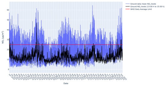
Figure 1.
NO2 daily average concentrations from MAMC ground sensors (blue line). NO2 average ground sensor measurement for the 2-h period of the Sentinel-5P satellite (13:00 to 15:00 LST).
Additionally, Figure 1 shows the average NO2 measure for the 2-h period of the satellite. For data seasonality, the winter months present higher levels of concentrations. Moreover, the data trend is similar to that of the whole day NO2 average.
The geographical setup of the MAMC significantly contributes to air pollution issues, particularly the accumulation of NO2. The city’s location in a high-altitude basin surrounded by mountains to the west, south, and east traps pollutants close to the ground, as the basin’s configuration restricts wind flow at ground level, preventing the dispersion of pollutants. Figure 2 shows the urban and green areas of the MAMC. In this figure, we can see that, as stated before, the west and south-east are conformed by the presence of green areas. Consequently, understanding the spatial and temporal variations of NO2 within such a complex urban environment needs the integration of data from multiple sources, including satellite observations, meteorological data, and ground-based measurements. This comprehensive approach is essential for developing robust predictive models that can accurately reflect the intricate dynamics of air pollution in the MAMC.
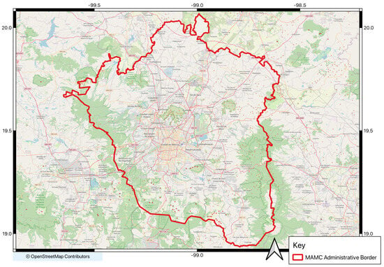
Figure 2.
Detailed map of the MAMC, showing roads, urban settlements, and green areas.
The methodology of the study was divided into three main phases. The initial phase involved directly applying the pre-trained model, developed for the MCM, to a set of ground sensor locations within the MAMC. This was carried out to test the pre-trained model’s performance in a different geographical and environmental setting without any modifications. In the second phase, the study incorporated the ABLH, along with the previously considered meteorological variables, to retrain the model but also specifically used data from the MCM. The inclusion of this additional variable was intended to enhance the model’s performance and its generalizability to diverse urban environments. With it, we address the unique topographical and atmospheric conditions that could be present in regions different from the MCM. This approach ensures a comprehensive evaluation of the model’s adaptability and robustness across different urban settings. In the final phase, we compared our model’s performance with TimeGPT. Figure 3 shows the general workflow to train, test, and select the model with the best performance by using the output’s RMSE.
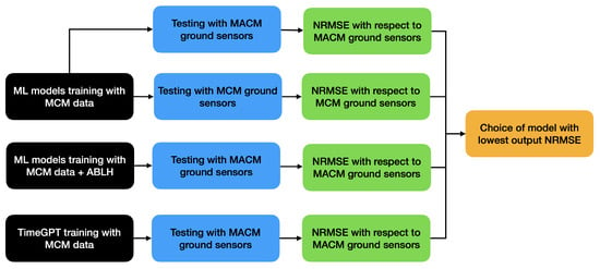
Figure 3.
Workflow to train and test output from models to select the one with the best performance.
The results indicate promising model adaptability to the conditions of the MAMC, with initial RMSE values lower or equal to the data’s standard deviation. This suggests robust performance in handling varying pollution sources and atmospheric dynamics. When retraining using data with the new atmospheric variables, the results show negligible performance improvement, indicating that further reprocessing and retraining of the original model is not needed. The model that was originally trained also performs significantly better than the solution proposed using TimeGPT. This research underscores the potential of integrating satellite observations and ML to create scalable and reliable air quality monitoring systems. It is particularly beneficial for LMICs, where traditional ground-based monitoring is limited. The findings aim to contribute to global efforts to improve air quality management and protect public health.
The structure of this article is organised as follows: Section 2 provides a detailed overview of the study area, data sources, and the methodology employed, including the integration of remote sensing data and ML techniques. In Section 3, we present the results of our analysis, highlighting the spatial and temporal patterns of NO2 concentrations and the model’s performance metrics. Section 3 also discusses the implications of our findings, emphasising the influence of meteorological factors and the potential applications of our model in air quality management. Finally, Section 4 concludes the article with a summary of key insights, the potential limitations of the study, and suggestions for future research directions.
2. Materials and Methods
2.1. Ground-Based NO2 Measurements
Mexico is a country subdivided into 32 administrative states. The area covered by the MAMC encompasses two states, the state of Mexico City and partially The State of Mexico. Inside this area, ground-based NO2 measurements are sourced from the SIMAT network, which historically operates a total of 32 air quality monitoring stations across the MAMC. For this work, only 10 of these stations were used. A total of 22 out of the 32 stations were disregarded because either they stopped working after the year 2021 or had inactive periods of more than 1 year. Figure 4 shows the area of interest (AoI) delimited by a red contour. In blue are the Sentinel-5P satellite pixels, and in black crosses are the locations of the NO2 ground stations. Similar to the MCM, the stations are dispersed, but most of them are located in the central part of the MAMC. This means that there were no stations present in the north and eastern parts of the AoI.
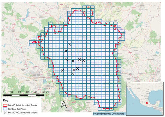
Figure 4.
Location of NO2 ground stations provided by Mexico City’s local authorities.
The NO2 ground stations provide hourly concentration data in micrograms per cubic meter (µg/m3). This data is essential for the validation of our ground estimation model. The dataset spanned from January 2019 to January 2023. In order to offer a comprehensive temporal coverage equivalent to the one used for the MCM, we used an average ground measurement of the time of the satellite passage (Section 2.2). This means that we only used a single average measurement of the NO2 average from 12:00–15:00 UTC-6.
Ground-based NO2 measurements in the MAMC are conducted using chemiluminescence analysers, which are the standard instruments for measuring nitrogen dioxide levels. These analysers detect NO2 via its reaction with ozone, which produces a chemiluminescent reaction (light emission) that can be measured. The intensity of the emitted light is directly proportional to the NO2 concentration, allowing for precise quantification. This method is widely recognised for its accuracy and reliability in detecting NO2 at various concentration levels [18,19].
In order to ensure data quality, SIMAT employs several validation and quality assurance procedures:
- Regular maintenance and calibration: Ground stations undergo routine maintenance and calibration to ensure the accuracy and reliability of the instruments.
- Data validation: Raw analyser data are subjected to validation processes to detect and correct anomalies or errors.
- Intercomparison studies: In some cases, data from ground stations have been compared and used following data from other monitoring networks and satellite observations to ensure consistency and accuracy [18].
As previously mentioned, to ensure the reliability of our ML model’s estimates of ground-level NO2 concentrations, we employed a validation process using ground-based sensor data. This involved systematically comparing the predicted NO2 values generated by the model with the actual measurements obtained from a network of ground monitoring stations distributed throughout the MAMC.
2.2. Satellite Data: Sentinel-5P
For this study, Sentinel-5P data were employed to estimate ground-level NO2 concentrations in the MAMC. This satellite measures the NO2 tropospheric column with global coverage and a daily temporal resolution. Figure 4 illustrates the NO2 pixels of the Sentinel-5P TROPIMI as captured over the MAMC.
The Sentinel-5P satellite is part of the Copernicus program managed by the European Space Agency (ESA) in collaboration with the Netherlands Space Office (NSO). This satellite was launched with the primary goal of filling the data gap between the older missions, such as OMI (Ozone Monitoring Instrument) from the National Aeronautics and Space Administration (NASA) and the upcoming Sentinel-5 missions. Sentinel-5P carries a single instrument, the TROPOMI, developed by the Netherlands Aerospace Centre (NLR) and Airbus Defence and Space [6]. TROPOMI is a spectrometer that measures sunlight reflected and scattered by the Earth’s atmosphere and surface. It covers a wide spectral range from ultraviolet to shortwave infrared wavelengths, enabling the observation of a variety of atmospheric constituents, including NO2, ozone, sulfur dioxide, carbon monoxide, methane, and aerosols. This extensive spectral coverage is crucial for comprehensive atmospheric analysis and allows for high-precision monitoring of air quality [6,20].
Since becoming operational, Sentinel-5P has consistently met or exceeded these accuracy requirements, demonstrating high reliability in its measurements [21]. The validation of Sentinel-5P data involves several rigorous methods, including comparisons with ground-based stations, aircraft campaigns, and inter-satellite comparisons. Ground-based validation compares satellite data with measurements from various ground-based instruments such as multi-axis differential optical absorption spectroscopy (MAX-DOAS) instruments, Pandonia Global Network, and OMI [22]. These ground-based stations provide high-accuracy data that serve as a benchmark for validating satellite observations [21,23].
Aircraft validation involves comparing satellite data with measurements obtained from aircraft campaigns. These campaigns utilise in situ instruments and remote sensing instruments aboard aircraft to measure NO2 concentrations at different altitudes, providing a vertical profile that complements the satellite data. Intersatellite comparisons are conducted by comparing Sentinel-5P data with measurements from other satellites that monitor atmospheric NO2, such as OMI and GOME-2. These intercomparisons help in understanding any systematic biases and ensuring consistency across different satellite missions [24].
In addition to these validation methods, the Sentinel-5P mission team employs several other approaches to assess data quality, such as internal consistency checks, trend analysis, and intercomparison with models. The following table summarizes the validation methods and their accuracy metrics [21]:
Sentinel-5P data are open and free to access by anyone with an internet connection. The ESA makes it accessible through various platforms, including the following:
- Copernicus Data Space: Provides free access to Sentinel-5P data and other Copernicus data products https://dataspace.copernicus.eu (accessed on 9 July 2024).
- ESA Earth Observation Data Services: Data and Information Access Services (DIAS) provide a wide range of Earth observation data, as well as processing and analysis services https://www.copernicus.eu/en/access-data/dias (accessed on 9 July 2024).
To obtain Sentinel-5P images for the MAMC, we utilised the Copernicus application programming interface (API): https://documentation.dataspace.copernicus.eu/APIs.html (accessed on 11 July 2024). Given the extensive dataset required—spanning four years and totalling nearly 1.5 terabytes of data for the MAMC, we developed a specialised Python pipeline to facilitate automated batch downloads. This pipeline was designed to enhance efficiency and ensure the completeness of data acquisition. The pipeline operates by allowing users to specify the desired product, period, and area of interest. Upon receiving these parameters, it queries the Copernicus Hub, which responds with a comprehensive list of files available for download. The program then cross-references this list with the files already downloaded to identify any missing data. Subsequently, it downloads the necessary files one by one, ensuring that all required data are acquired without duplication or omission. This approach marks a significant improvement over previous methods, such as using DIAS services, as it leverages a free service without quotas or limitations. The efficiency of this system is further highlighted by its ability to manage interruptions caused by the data provider. Our pipeline addresses this by seamlessly resuming downloads from the point of interruption, thus avoiding the time-consuming task of manually tracking download progress. By automating the data acquisition process, this pipeline significantly reduces the potential for human error and ensures that no data are missed. The systematic and reliable nature of this method not only accelerates the download process but also ensures a higher level of data integrity. This pipeline was crucial for our comprehensive analysis of NO2 concentrations across the MAMC, enabling us to achieve a continuous dataset with no time gaps. This was necessary for accurate atmospheric modelling and analysis.
2.3. Meteorological Data: ERA5
ERA5 (https://cds.climate.copernicus.eu/cdsapp#!/dataset/reanalysis-era5-single-levels accessed on 11 February 2024) provides detailed and high-resolution meteorological data that are essential for understanding and modelling atmospheric processes affecting NO2 dispersion. The ERA5 dataset includes hourly estimates of a wide range of atmospheric parameters. For this study, the key meteorological parameters included near-surface temperature at 2 m above the ground, wind speed and direction at 10 m above the ground, surface relative humidity, total precipitation, and surface atmospheric pressure.
In addition to these parameters, which were used in past studies, we also included the ABLH provided by the ERA5 reanalysis. The ABLH is the lowest portion of the troposphere that is directly influenced by the surface beneath it. The thickness of this layer, denoted as ABLH, is a crucial parameter in various applications such as air pollution modelling and weather forecasting. In environmental contexts, the ABL height defines the volume of air in which pollutants are dispersed. Hence, the precise determination of the ABLH is vital for accurately modelling air quality, including the processes of pollutant transport, dispersion, and removal. Moreover, ABL height serves as an essential scaling factor for normalising boundary layer variables such as fluxes and vertical gradients of wind, potential temperature, and moisture, which are critical for both model-based and observational analyses. In addition, it plays a significant role in nonlocal turbulence closures employed in climate and weather forecasting models, such as the National Center for Atmospheric Research (NCAR) Community Climate Model and the National Centers for Environmental Prediction (NCEP) medium-range forecasting model [25].
The time span of these parameters was from January 2019 to January 2023, and this was accessed through the ECMWF Climate Data Store. The data were aggregated to match the temporal resolution of the Sentinel-5P measurements, typically occurring around local noon [26]. By aggregating ERA5 data into daily averages, we ensure that the data matches the temporal resolution of the satellite observations. This alignment allows us to capture the meteorological conditions that significantly impact NO2 levels. Temperature, wind, humidity, precipitation, pressure, and ABLH are critical variables that affect the dispersion and chemical reactions of NO2 in the atmosphere. By integrating these parameters, we can enhance the predictive power of our models, allowing for more accurate estimations of ground-level NO2 concentrations across different temporal and spatial scales.
2.4. Data Processing
Due to the nature of the data coming from different sources, the processing and harmonisation required substantial effort. In order to achieve this, we utilised the preprocessing algorithm developed in our previous work [8], which significantly facilitated the handling of Sentinel-5P and ERA5 datasets. However, the ground sensors of the MAMC, being new and structurally different from those used in Milan, required preprocessing from scratch. In the following sections, we will describe the specific steps involved in processing the Sentinel-5P, ERA5, and MAMC ground sensor datasets. This comprehensive approach ensures that the resulting datasets are robust, reliable, and ready for integration into the modelling framework.
2.4.1. Satellite Data Processing
Sentinel-5P images are provided at Level 2 (L2). Although L2 already provides the NO2 tropospheric column, some pixels must be removed to ensure the reliability of the data. Initially, pixels with cloud coverage were excluded using quality assurance values provided within the dataset, retaining only high-quality measurements (above 0.75 quality assurance values). The quality assurance values we used are the ones suggested by the ESA in their technical literature [23]. These preprocessing steps are critical for ensuring the integrity of the data used in subsequent analyses, as cloud cover can significantly distort satellite observations. By using the HARP tool from the atmospheric toolbox (https://atmospherictoolbox.org/harp/ accessed on 28 October 2023) provided by ESA, we filtered out the low-quality pixels, binned the data into a regular grid and reduced the spatial extent to the interest area. These steps facilitate seamless integration with other data sources.
In order to estimate the ground-level NO2 concentrations, we considered the time resolution of the Sentinel-5P for the rest of the datasets. According to Figure 5, Sentinel-5P overpasses occur between 13:00 and 15:00 local time (19:00 and 21:00 UTC). Therefore, the ERA5 and ground sensor network measurements were averaged every day in these 2 h. Figure 6 illustrates the coefficients of variation for each of the ERA5 meteorological variables during the satellite overpass period. We observe that all variables, except for the wind components, exhibit less than 2% variation relative to their overall mean. The wind ‘U’ and ‘V’ components also have their first and third quartiles—representing 50% of the data—below a 2% variation. This indicates that averaging data over these 2 h is appropriate, as it captures a representative and stable sample of the meteorological conditions during the satellite’s overpass.
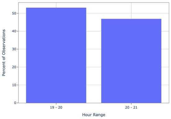
Figure 5.
Satellite passage times over the MAMC. The times are indicated in UTC-6.
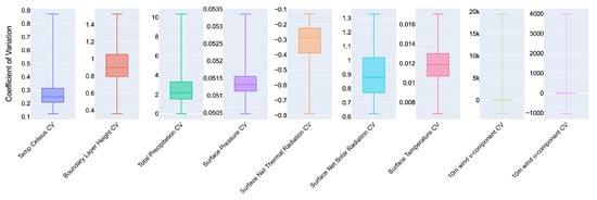
Figure 6.
Coefficients of variation for each of the variables used in the ML model in the 2-h satellite overpass period.
2.4.2. Meteorological Data Aggregation
ERA5 meteorological data were aggregated into two datasets. The first dataset was synchronised with the temporal resolution of Sentinel-5P observations, leading us to calculate the daily averages for each ERA5 meteorological parameter during the satellite’s overpass time. This step is crucial for creating a consistent and comparable dataset that accurately reflects the meteorological conditions influencing NO2 levels during satellite observations. Additionally, daily aggregation smooths out short-term fluctuations, resulting in a more stable dataset for modelling purposes.
The second dataset involved averaging hourly data from the time preceding the satellite overpass. This process was completed in two steps. First, we calculated the average ERA5 measurements from 00:00 to 13:00 local time. Next, we computed the average ERA5 measurements from 15:00 to 23:59 of the previous day. Once these two averages were obtained, they were further averaged to produce a final attribute for each meteorological value corresponding to the preceding period of the satellite overpass. This “previous day” parameter was included because it is highly correlated with the NO2 ground measurements [8].
2.4.3. Ground-Based Data Synchronisation
For the ground sensors of the MAMC, the process began with data acquisition and initial formatting. Unlike the Milan sensors, which had a well-established data structure, the MAMC sensors required the development of new preprocessing routines. This included standardising the data formats and restructuring them to have the same input format as those of the MCM to be used with the pretrained model.
The hourly ground-based NO2 measurements were averaged from 13:00 to 15:00 local time to create daily values that matched the temporal resolution of the passage of the satellite. Additionally, spatial interpolation using the nearest neighbours method was employed to align the grid cells used for the satellite and meteorological data with the ground measurements. Nearest neighbours are a straightforward interpolation technique that assigns values to grid cells based on the closest observed data points. This method ensures that the spatial variability of NO2 concentrations is adequately represented across the study area, enhancing the robustness of the integrated dataset. By using nearest neighbours, we maintained a computationally efficient approach that reliably interpolates spatial data, ensuring a consistent and accurate representation of NO2 levels throughout the study region [27].
As we mentioned in the previous paragraphs, the inclusion of NO2 values from Sentinel-5P provides direct measurements of atmospheric NO2. These have the highest correlation (Table 1) among all the features, making them essential for estimating ground-level concentrations. Meteorological parameters, such as temperature, wind, humidity, precipitation, and pressure, influence the dispersion and chemical reactions of NO2 in the atmosphere. Temporal variables help account for patterns in human activity and natural processes that affect NO2 levels. By carefully selecting and engineering these features, we enhance the predictive power of the models, allowing them to accurately capture the complex interactions and dependencies that govern NO2 concentrations.

Table 1.
Pearson correlation coefficients of ERA5 variables and Sentinel-5P with respect to ground-level atmospheric NO2.
2.5. Feature Engineering
Feature engineering is a critical step in the development of ML models, involving the selection and transformation of relevant variables to enhance model performance. In this study, key features were selected from the Sentinel-5P satellite data and ERA5 meteorological data based on the Pearson correlation coefficient for ground-level atmospheric NO2 measurements at the time of passage of the satellite. These features included NO2 column density from Sentinel-5P, surface temperature, wind speed and direction, humidity, surface pressure, precipitation, and ABLH from ERA5.
Table 1 presents the Pearson correlation coefficients for ground-level atmospheric NO2. The first column lists the variable being measured, either Sentinel-5P or ERA5 meteorological data. The second column displays the Pearson correlation coefficient between this variable’s average values across the MCM and the ground average NO2 measurements. The third column shows the Pearson correlation coefficient for the same variables but for the MAMC. As indicated in the table, the ERA5 meteorological variables and Sentinel-5P data generally exhibit lower correlations with ground-level NO2 measurements in MAMC compared to MCM. This suggests that the relationship between these variables and NO2 levels varies significantly between the two regions, possibly due to differing environmental and atmospheric conditions. Even though the correlations for the MAMC are lower than those for the MCM, we can observe that the selected variables are still the ones with the strongest Pearson correlation coefficient.
In order to reduce the number of variables and improve model performance, we originally decided to use the Pearson correlation coefficient. We chose values with a correlation higher than 0.5 as an absolute value. Although the ML model was not retrained with the MAMC data, this information can be useful for analysing the results and explaining possible behaviours. By taking these points in mind, the following variables were the ones used to train the original model on the MCM:
- Ground NO2
- Satellite NO2
- Current Temp Celsius
- Current Surface Net Solar Radiation
- Current Surface Pressure
- Previous Temp Celsius
- Previous Surface Net Solar Radiation
2.6. Model Training and Validation
Originally, the MCM dataset was divided into training and validation sets using an 80–20 split. This was carried out in two ways: chronologically (with data from 2019 to 2022 used for training and data from 2023 used for validation) and randomly. As seen in our previous work, the method that had the best results was random splitting. For our model to be appropriately evaluated in the MAMC, we used the same testing dates as in the MCM, evenly distributed across the testing period. Moreover, we applied normalisation to ensure that the models were not affected by the different scales of the input features. This involved standardising each feature to have zero mean and unit variance, which is particularly important for models such as SVR and neural networks that are sensitive to the scale of input data.
Based on the findings presented in Table 1, which indicate a strong correlation between ABLH and the model output (greater than 0.5 for the MCM), we decided to enhance the original model by incorporating data from the ABLH of ERA5 in our retraining process.
TimeGPT
Built on a transformer-based structure, TimeGPT (https://docs.nixtla.io) primarily focuses on predicting future time steps based on historical data. A key feature is a self-attention mechanism, enabling the model to weigh the importance of different time steps in the input sequence, which helps capture the long-range dependencies common in time series data [13,28].
The model undergoes two-phase training: pretraining and fine-tuning. In pretraining, TimeGPT learns generic temporal patterns from a large dataset of diverse time series data. Fine-tuning adapts the model to the unique characteristics of the target data, enhancing forecasting accuracy. Time embeddings encode temporal information such as time of day, day of the week, and seasonality, providing context for understanding temporal patterns. The model also uses covariates, such as economic indicators or weather conditions, which may influence the target variable [13,28].
The versatility of TimeGPT allows it to be used across various domains that require accurate time series forecasting. For instance, meteorological departments can use TimeGPT to forecast weather, temperature, and precipitation based on historical data. It can aid in natural disaster prediction by forecasting events such as hurricanes and floods. In healthcare, TimeGPT can predict disease outbreaks by analysing temporal patterns in health data [13,28].
In our study on NO2 concentrations in the MAMC, TimeGPT can significantly enhance forecasting accuracy. The integration involves collecting historical NO2 measurements, meteorological data (temperature, humidity, and wind speed), and satellite data from Sentinel-5P as additional covariates. Fine-tuning adapts the model to local temporal patterns and trends, improving its forecasting performance. Once trained, TimeGPT can estimate ground-level atmospheric NO2 concentrations.
3. Results and Discussion
As stated in Section 1, the first phase of this work consisted of testing and validating the model trained using only data from the MCM from 1 January 2019 to 27 September 2022. The features used for the training of this model were Satellite NO2, Current Temp Celsius, Current Surface Net Solar Radiation, Current Surface Pressure, Previous Temp Celsius, and Previous Surface Net Solar Radiation. The model that had the best performance was a combination of multi-layer preceptor regressor and support vector regressor by using Scikit-Learn (https://scikit-learn.org/).
Columns 1 and 2 of Table 2 and Table 3 show the NRMSE for the MCM and for the MAMC using the original model. As expected, the base model performs better in the Milano area than in the MAMC. The reason for this is that (as mentioned in Section 2.6) the model was trained exclusively with data from the MCM area. Even though the NRMSE of the MAMC was higher than that of the MCM, the values are lower than those of the standard deviation (more than 15% lower). This indicates that even if the atmospheric and topographical conditions and the ground-level measurement sensors are different between these two urban areas, the results are still within an acceptable range.

Table 2.
NRMSE (%) obtained for the atmospheric NO2 ground-level estimation for each of the MCM sensor locations.

Table 3.
NRMSE (%) obtained for the atmospheric NO2 ground-level estimation for each of the MAMC sensor locations.
Additionally, in the third column of Table 2 and Table 3, we observe the NRMSE results for the retrained model. The retrained model changes from the original in the sense that it was trained with the ABLH and considers the years from 2019 to 2022 fully. This means that the dataset now includes an additional variable with a high correlation with ground-level NO2 for the MCM. Although some of the stations have a lower NRMSE compared to the original model, integrating the ABLH into our model does not contribute to lowering the general error of the estimations.
Due to the negligible or nonexistent improvement observed with the retrained model, we decided to utilise only the original model for the subsequent results. Figure 7 illustrates the time series plots of the model estimations versus the actual ground truth measurements. In blue, we can observe the ground measurements provided by the network testing dataset of SIMAT, and in orange, we can see the estimations produced by our trained model for the same dates. Consistent with previous studies [8], the overall trend in the estimation plots closely mirrors that of the ground measurements. However, the largest errors were observed on days with peak values, which proved more challenging to estimate accurately. This pattern is also evident in the estimations produced by the MCM, where certain regions of the plots show an underestimation by the model. This underestimation is particularly present during periods when ground-level NO2 concentrations peak, as previously mentioned.
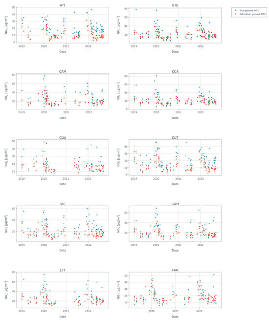
Figure 7.
Original base model estimations for the MAMC at the time of passage of the satellite versus ground truth at the time of passage of the satellite.
The consistency in the results was also confirmed by the correlation between the ground truth and the model’s estimation. These have an average Pearson correlation coefficient of 0.55, a trend which can also be observed in Figure 8.
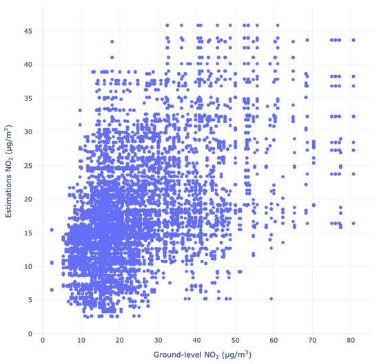
Figure 8.
Scatter plot of NO2 ground-level measurements from SIMAT and the model’s estimations.
Land use delineates the activities and constructions on a given piece of land, identifying the types of communities, environments, or settlements that are established. It includes human efforts to exploit and adapt the landscape for various purposes. Consequently, land-use change reflects the transformation of the natural landscape driven by human activities, highlighting the land’s role and function in socio-economic contexts. This concept is often utilised in mapping to classify land types and gain a better understanding of phenomena occurring in specific urban areas. In our study, land-use classification aids in explaining the behaviour of estimations at each ground station according to the type of activities developed in a specific location of a city. For our work, we used the Global Intra-Urban Land Use classification [29]. The following categories are proposed by this work:
- Open Space: Includes public open areas, vacant land, and water bodies. These areas are designated for recreation or conservation or remain undeveloped, offering ecological benefits and leisure opportunities.
- Non-residential Areas: Encompasses commercial, office, industrial, civic, and transportation hubs and networks other than roads. These zones are utilised for business activities, industrial operations, public services, and transport infrastructure.
- Atomistic Settlements: Areas developed without formal planning, featuring irregular layouts and non-uniform parcel sizes and road widths. These areas evolved organically over time.
- Informal Land Subdivision: Areas with informally planned layouts marked by visible but inconsistent infrastructure, variable parcel sizes, and road widths. These areas often lack formal approval and standardised infrastructure.
- Formal Land Subdivisions: Areas planned with municipal approval, showcasing consistent infrastructure quality, standardised parcel sizes, and road widths. These zones adhere to municipal regulations and include paved roads, streetlights, and sidewalks.
- Housing Projects: Developments where land subdivision and home construction follow a unified plan, resulting in similar structures and layouts. These projects range from large apartment complexes to uniform suburban housing, typically developed by a single entity.
Figure 9 displays the location of each station and the assigned land-use category. The map also distinguishes stations with a mean RMSE lower than the general median in blue and those with a mean RMSE higher than the general median in red. Contrary to expectations, land use in this context does not clarify the magnitude of error in the estimations. Instead, it reveals that stations with the lowest error are situated in the most urbanised and central parts of the city, where traffic intensity is higher. This suggests that the model performs better at estimating NO2 concentrations in densely populated urban scenarios or high-traffic roads. This suggests that the model is more effective at estimating concentrations at source locations than in areas with significant NO2 transport. This conclusion is supported by the correlation between wind speed, wind direction, and NO2 concentrations (Table 1), indicating that wind has less influence on the results. This same effect can be observed in previous studies [7].
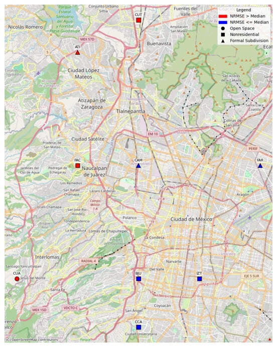
Figure 9.
MAMC stations with the type of land-use and colour coding for the global median for the time of passage of the satellite.
In order to ensure that the estimations align closely with the ground truth data, we performed a statistical comparison of their density distributions. We employed a density distribution comparison technique, visualised in Figure 10. This figure illustrates the relationship between the two sets of data points. Ideally, if the estimations and the ground truth are statistically similar, the points in the Q–Q plot should lie along a 45-degree reference line. In our analysis, the Q–Q plot shows an almost linear relationship, indicating that the two distributions are similar. This linearity implies that the estimations do not just approximate the ground truth at a general level but match closely across the entire range of values. Such a result confirms that our estimation model is robust and capable of accurately reflecting real-world NO2 concentrations. Moreover, this analysis provides confidence in the model’s predictive capabilities, as the statistical similarity between the estimated and actual data suggests that the model can generalise well to new data. This consistency is essential for applications in air quality monitoring and forecasting, where reliable and precise data are necessary for informed decision-making and policy development.
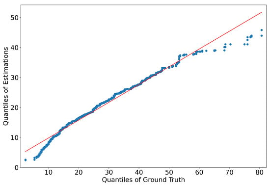
Figure 10.
Quantile–quantile plots, comparing the data distribution of the ML model estimation against the ground truth. The blue dots correspond to one quantile of the first distribution against the same quantile of the second distribution. The red line is used as a reference to represent an ideal linear relationship between the distributions.
Finally, we compared the performance of our original model to TimeGPT (Section 2.6). Table 4 and Table 5 show the comparison between our model (column 2) and that one using TimeGPT (column 3). As expected, it can be observed that the error for the TimeGPT model is significantly larger than our model. A possible explanation is that our model was specifically trained to estimate NO2 ground-level atmospheric concentrations at the time of the passage of the satellite. In contrast, TimeGPT was pretrained using a large amount of data and then adjusted to our model. This means that our model is more specialised in our study of interest.

Table 4.
NRMSE (%) obtained by using the original model and the TimeGPT model for the estimations in the MCM.

Table 5.
NRMSE (%) obtained by using the original model and the TimeGPT model for the estimations in the MAMC.
It is also important to highlight that, at the moment, TimeGPT has the possibility to perform estimations using multiple variables. Nevertheless, it has some restrictions. The most significant limitation that we found when using this model is that the data need to be continuous with no time gaps. By eliminating these time gaps, the data partially loses its seasonal behaviour. Additionally, TimeGPT requires that all the testing data sensors have the same amount of dates. Both of these constraints make the study lose its seasonality (as previously mentioned) and reduce the amount of data points for the testing period.
A critical review of the factors influencing NO2 concentrations reveals the importance of various meteorological and environmental variables. Temperature and solar radiation are particularly significant. It can be assumed that they influence the dispersion and transport of NO2 across different regions of the study area. Temperature also plays a vital role, as it can affect the rate of chemical reactions in the atmosphere, including the formation and degradation of NO2. Wind typically leads to the dispersion of pollutants. Wind directions can carry NO2 from emission sources to other areas, influencing the spatial distribution. Moreover, net solar radiation affects photochemical reactions that can alter NO2 levels throughout the day, particularly in urban environments where solar exposure varies due to building shading and other urban features.
In addition to meteorological factors, the topography and land use patterns significantly impact NO2 distribution. On the one hand, areas with high traffic density, industrial activities, and lower elevations are prone to higher NO2 concentrations due to the accumulation of emissions and limited dispersion. On the other hand, regions with more vegetation or at higher altitudes may experience lower NO2 levels due to natural absorption and dispersion processes. Our model accounts for these impact factors by incorporating a range of covariates, including meteorological data and land use classifications, to enhance the accuracy of NO2 concentration estimations. However, it is essential to consider that variations in these factors, especially in complex urban terrains such as the MAMC, may introduce challenges in modelling that could need further refinement to fully capture their influence on NO2 levels.
4. Conclusions
The research presented in this article provides a comprehensive analysis of ground-level NO2 concentrations using ML and remote sensing data, with a specific focus on the MAMC. Our study employed a model that was pretrained in previous works using data from the MCM. This model uses Sentinel-5P satellite data and ERA5 data as input. Ground-based measurements were used to evaluate the estimations. The integration of these data sources allowed us to address the spatial and temporal limitations of traditional ground-based monitoring systems, offering a more extensive and continuous approach to air quality assessment.
Our findings demonstrate that the ML model we developed is capable of estimating NO2 ground-level concentrations at the ground sensor locations at the time of the passage of the satellite (from 13:00 to 15:00 local time). The model’s performance was evaluated using several statistical metrics, including RMSE and NRMSE. Notably, the model was able to capture the spatial variability of NO2 across different regions of the MAMC.
One of the key insights from our analysis is the significant influence of meteorological factors on NO2 concentrations. Parameters such as temperature, wind speed, and net solar radiation were found to be crucial in determining NO2 dispersion and concentration levels. This underscores the importance of incorporating meteorological data into air quality models to enhance their predictive capabilities. Our study also revealed that NO2 estimations are notably better in regions with dense traffic and industrial activities, corroborating previous findings from previous works.
The temporal analysis of NO2 concentrations provided valuable insights into the di-urnal and seasonal patterns of pollution. We observed that seasonal variations indicated higher NO2 concentrations during the colder months, likely due to temperature inversions that trap pollutants near the ground.
Our study highlighted the potential of using remote sensing data for air quality monitoring in regions with limited ground-based infrastructure. The Sentinel-5P satellite, in combination with the ERA5 reanalysis model, proved to be an effective tool for estimating NO2 data. The open accessibility of the data offers a valuable resource for researchers and policymakers in low- and middle-income countries, where financial and technical constraints often limit the implementation of comprehensive air quality monitoring networks.
In conclusion, this research demonstrates the efficacy of combining ML with remote sensing data to estimate ground-level atmospheric NO2 concentrations. Our model provides a scalable and cost-effective solution for monitoring air quality, particularly in urban areas with significant pollution challenges. The insights gained from this study can inform the development of more effective air quality management strategies and contribute to the broader efforts of mitigating the adverse health and environmental impacts of atmospheric pollution. Future work should focus on further refining the model and exploring its application to other pollutants and regions to enhance our understanding of urban air quality dynamics and support global efforts in combating air pollution.
Author Contributions
Conceptualisation, M.A.B. and J.R.C.J.; methodology, M.A.B. and J.R.C.J.; software, J.R.C.J.; validation, M.A.B. and J.R.C.J.; formal analysis, M.A.B. and J.R.C.J.; investigation, J.R.C.J.; resources, M.A.B.; data curation, J.R.C.J.; writing—original draft preparation, J.R.C.J.; writing—review and editing, M.A.B. and J.R.C.J.; visualisation, J.R.C.J.; supervision, M.A.B.; project administration, M.A.B.; funding acquisition, M.A.B. All authors have read and agreed to the published version of the manuscript.
Funding
This research was partially funded by the Italian Ministry of Education through the project of national interest (PRIN) “Geo-Intelligence for improved air quality monitoring and analysis (GeoAIr)” (project code: 202258ACSL-PE10).
Informed Consent Statement
Informed consent was obtained from all subjects involved in the study.
Data Availability Statement
Publicly available datasets were analyzed in this study. ERA5 data can be found here: https://cds.climate.copernicus.eu/cdsapp#!/dataset/reanalysis-era5-single-levels?tab=overview (accessed on 4 September 2024). SIMAT MAMC data can be found here: https://datos.cdmx.gob.mx/dataset/red-automatica-de-monitoreo-atmosferico (accessed on 4 September 2024). Python Jupyter Notebooks containing processing pipelines can be found here: https://github.com/rodrigocedeno/Ground-Level-NO2-ML-Rodrigo_Ce.git (accessed on 4 September 2024).
Conflicts of Interest
The authors declare no conflicts of interest.
Abbreviations
The following abbreviations are used in this manuscript:
| API | Application Programming Interface |
| AoI | Area of Interest |
| DIAS | Data and Information Access Services |
| ECMWF | European Centre for Medium-Range Weather Forecasts |
| ERA5 | Fifth-generation reanalysis dataset from ECMWF |
| EU | European Union |
| GOME-2 | Global Ozone Monitoring Experiment-2 |
| GPT | Generative Pre-training Transformer |
| LMIC | Low- and Middle-Income Countries |
| MAMC | Metropolitan Area of Mexico City |
| Max-DOAS | Multi-Axis Differential Optical Absorption Spectroscopy |
| MCM | Metropolitan City of Milan |
| MDPI | Multidisciplinary Digital Publishing Institute |
| ML | Machine Learning |
| NASA | National Aeronautics and Space Administration |
| NLR | Netherlands Aerospace Center |
| NO2 | Nitrogen Dioxide |
| NSO | Netherlands Space Office |
| OMI | Ozone Monitoring Instrument |
| SIMAT | Sistema de Monitoreo Atmosférico (Atmospheric Monitoring System) |
| TROPOMI | Tropospheric Monitoring Instrument |
| UTC | Coordinated Universal Time |
| WHO | World Health Organisation |
References
- Ma, Y.; Nobile, F.; Marb, A.; Dubrow, R.; Stafoggia, M.; Breitner, S.; Kinney, P.L.; Chen, K. Short-Term Exposure to Fine Particulate Matter and Nitrogen Dioxide and Mortality in 4 Countries. JAMA Netw. Open 2024, 7, e2354607. [Google Scholar] [CrossRef] [PubMed]
- Trushna, T.; Tiwari, R.R. Establishing the National Institute for Research in Environmental Health, India. Bull. World Health Organ. 2022, 100, 281–285. [Google Scholar] [CrossRef] [PubMed]
- Tyagi, S.; Chaudhary, M.; Ambedkar, A.K.; Sharma, K.; Gautam, Y.K.; Singh, B.P. Metal Oxide Nanomaterials based sensors for monitoring environmental NO2 and its impact on plant ecosystem: A Review. Sens. Diagn. 2022, 1, 106–129. [Google Scholar] [CrossRef]
- Piccoli, A.; Agresti, V.; Balzarini, A.; Bedogni, M.; Bonanno, R.; Collino, E.; Colzi, F.; Lacavalla, M.; Lanzani, G.; Pirovano, G.; et al. Modeling the Effect of COVID-19 Lockdown on Mobility and NO2 Concentration in the Lombardy Region. Atmosphere 2020, 11, 1319. [Google Scholar] [CrossRef]
- Reimann, S.; Wegener, R.; Claude, A.; Sauvage, S. Updated Measurement Guideline for NOx and VOCs; Actris: Dübendorf, Switzerland, 2018. [Google Scholar]
- Kramer, H.J. Copernicus: Sentinel-5P (Precursor—Atmospheric Monitoring Mission); eoPortal Directory: Paris, France, 2022. [Google Scholar]
- Cedeno Jimenez, J.R.; Oxoli, D.; Brovelli, M.A. Enabling Air Quality Monitoring with the Open Data Cube: Implementation for Sentinel-5P and Ground Sensor Observations. Int. Arch. Photogramm. Remote Sens. Spat. Inf. Sci. 2021, 46, 31–36. [Google Scholar] [CrossRef]
- Cedeno Jimenez, J.R.; Pugliese Viloria, A.D.J.; Brovelli, M.A. Estimating Daily NO2 Ground Level Concentrations Using Sentinel-5P and Ground Sensor Meteorological Measurements. ISPRS Int. J.-Geo-Inf. 2023, 12, 107. [Google Scholar] [CrossRef]
- World Health Organization. Global Air Quality Database App: App for Exploring Air Quality in Countries; WHO Global Air Quality Database (Update 2018) Edition; World Health Organization: Geneva, Switzerland, 2018. [Google Scholar]
- Johnston, M. List of the World’s Largest Cities by Population; Encyclopedia Britannica: Chicago, IL, USA, 2024. [Google Scholar]
- Calderón-Garcidueñas, L.; Kulesza, R.J.; Doty, R.L.; D’Angiulli, A.; Torres-Jardón, R. Megacities air pollution problems: Mexico City Metropolitan Area critical issues on the central nervous system pediatric impact. Environ. Res. 2015, 137, 157–169. [Google Scholar] [CrossRef] [PubMed]
- Hinojosa-Baliño, I.; Infante-Vázquez, O.; Vallejo, M. Distribution of PM2.5 Air Pollution in Mexico City: Spatial Analysis with Land-Use Regression Model. Appl. Sci. 2019, 9, 2936. [Google Scholar] [CrossRef]
- Garza, A.; Mergenthaler-Canseco, M. TimeGPT-1. arXiv 2023, arXiv:2310.03589. [Google Scholar]
- GobMx. Valle de México: Economía, Empleo, Equidad, Calidad de Vida, Educación, Salud y Seguridad púBlica. 2024. Available online: https://www.economia.gob.mx/datamexico/es/profile/geo/valle-de-mexico (accessed on 23 June 2024).
- ADIP. Acerca de la Ciudad de México|Your Cultural Destination of the Decade. 2024. Available online: https://mexicocity.cdmx.gob.mx/e/about/about-mexico-city/?lang=es (accessed on 15 June 2024).
- WHO. What Are the WHO Air Quality Guidelines? WHO: Geneva, Switzerland, 2021.
- Agencia Digital de Innovación Pública. Portal de Datos Abiertos de la CDMX. 2023. Available online: https://datos.cdmx.gob.mx/ (accessed on 16 June 2024).
- SIMAT. Informe Bimestral de la Calidad del Aire; Mexico City Atmospheric Monitoring System (SIMAT): Ciudad de Mexico, Mexico, 2002. [Google Scholar]
- Molina, L.T.; Velasco, E.; Retama, A.; Zavala, M. Experience from Integrated Air Quality Management in the Mexico City Metropolitan Area and Singapore. Atmosphere 2019, 10, 512. [Google Scholar] [CrossRef]
- European Commission. Level-0 Processing and Products; European Commission: Brussels, Belgium, 2021. [Google Scholar]
- Langen, J.; Meijer, Y.; Veihelmann, B.; Ingman, P. Copernicus Sentinels 4 and 5 Mission Requirements Traceability Document; ESA: Noordwijk, The Netherlands, 2017. [Google Scholar]
- CAMPCS; ESA. Sentinel-5P Mission Performance Centre Quarterly Validation Report; Issue 23.00.00; Technical Report; Copernicus Atmospheric Mission Performance Cluster Service: Brussels, Belgium, 2024. [Google Scholar]
- European Commission. Products and Algorithms; European Commission: Brussels, Belgium, 2021. [Google Scholar]
- ESA. Validation—Sentinel-5P Technical Guide—Sentinel Online. 2023. Available online: https://copernicus.eu/technical-guides/sentinel-5p/validation (accessed on 28 October 2023).
- Dai, C.; Wang, Q.; Kalogiros, J.A.; Lenschow, D.H.; Gao, Z.; Zhou, M. Determining Boundary-Layer Height from Aircraft Measurements. Bound.-Layer Meteorol. 2014, 152, 277–302. [Google Scholar] [CrossRef]
- Hersbach, H.; Bell, B.; Berrisford, P.; Hirahara, S.; Horányi, A.; Muñoz-Sabater, J.; Nicolas, J.; Peubey, C.; Radu, R.; Schepers, D.; et al. The ERA5 global reanalysis. Q. J. R. Meteorol. Soc. 2020, 146, 1999–2049. [Google Scholar] [CrossRef]
- Altman, N.S. An Introduction to Kernel and Nearest-Neighbor Nonparametric Regression; The American Statistician: Riverside, CA, USA, 1992; Volume 46. [Google Scholar] [CrossRef]
- Nixtla. TimeGPT Documentation. 2024. Available online: https://docs.nixtla.io (accessed on 23 May 2024).
- Guzder-Williams, B.; Mackres, E.; Angel, S.; Blei, A.M.; Lamson-Hall, P. Intra-urban land use maps for a global sample of cities from Sentinel-2 satellite imagery and computer vision. Comput. Environ. Urban Syst. 2023, 100, 101917. [Google Scholar] [CrossRef]
Disclaimer/Publisher’s Note: The statements, opinions and data contained in all publications are solely those of the individual author(s) and contributor(s) and not of MDPI and/or the editor(s). MDPI and/or the editor(s) disclaim responsibility for any injury to people or property resulting from any ideas, methods, instructions or products referred to in the content. |
© 2024 by the authors. Licensee MDPI, Basel, Switzerland. This article is an open access article distributed under the terms and conditions of the Creative Commons Attribution (CC BY) license (https://creativecommons.org/licenses/by/4.0/).