Article

A Space Object Optical Scattering Characteristics Analysis Model Based on Augmented Implicit Neural Representation

by
Qinyu Zhu
1,
Can Xu
1,
Shuailong Zhao
1,
Xuefeng Tao
1,
Yasheng Zhang
1,*,
Haicheng Tao
1,
Xia Wang
2 and
Yuqiang Fang
1
1
National Key Laboratory of Laser Technology, Space Engineering University, Beijing 101416, China
2
Institute of Tracking and Communication Technology, Beijing 100094, China
*
Author to whom correspondence should be addressed.
Remote Sens. 2024, 16(17), 3316; https://doi.org/10.3390/rs16173316
Submission received: 12 August 2024 / Revised: 22 August 2024 / Accepted: 5 September 2024 / Published: 6 September 2024
(This article belongs to the Section Satellite Missions for Earth and Planetary Exploration)

Abstract

:
The raw data from ground-based telescopic optical observations serve as a key foundation for the analysis and identification of optical scattering properties of space objects, providing an essential guarantee for object identification and state prediction efforts. In this paper, a spatial object optical characterization model based on Augmented Implicit Neural Representations (AINRs) is proposed. This model utilizes a neural implicit function to delineate the relationship between the geometric observation model and the apparent magnitude arising from sunlight reflected off the object’s surface. Combining the dual advantages of data-driven and physical-driven, a novel pre-training procedure method based on transfer learning is designed. Taking omnidirectional angle simulation data as the basic training dataset and further introducing it with real observational data from ground stations, the Multi-Layer Perceptron (MLP) parameters of the model undergo constant refinement. Pre-fitting experiments on the newly developed S−net, R−net, and F−net models are conducted with a quantitative analysis of errors and a comparative assessment of evaluation indexes. The experiment demonstrates that the proposed F−net model consistently maintains a prediction error for satellite surface magnitude values within 0.2 m V , outperforming the other two models. Additionally, preliminary accomplishment of component-level recognition has been achieved, offering a potent analytical tool for on-orbit services.

Graphical Abstract

1. Introduction

Advancements in technology have driven humanity to expand its exploration from the surface of the Earth to the vast expanse of space. Various artificial space objects, such as earth observation satellites and manned spacecraft, are exposed to threats from space debris and other space objects while performing their missions. To safeguard space interests and ensure space security, it is essential to acquire the current operational status of space objects and predict their future activity trends. Consequently, space object characterization methods that primarily rely on optical detection have become crucial technologies for on-orbit servicing [1].
The optical characteristics of space objects provide a crucial foundation for the inversion of space object features, encompassing scattering characteristics, radiation characteristics, polarization characteristics, and imaging characteristics [2]. The optical scattering characteristics, in particular, reveal the intrinsic properties of the objects themselves. Accurately describing these characteristics is essential for enabling effective feature recognition and state prediction, playing a vital role in the identification of space object states, target recognition, and catalog management. According to the location of the sensors, observational methods can be divided into space-based and ground-based categories. Ground-based observations predominantly rely on ground-based telescope equipment to detect space objects. The photometric signal curve obtained from these observations is coupled with numerous factors such as the object’s orbit, mass, attitude, surface material, observation geometry, etc., which contains a large amount of important characteristic information of the space object [3].
Ground-based detection systems possess advantages such as freedom from engineering constraints, including foundation, quality and power consumption, as well as reduced complexity in implementation, etc. The ground-based optical detection system can monitor over long distances and simultaneously observe space objects in low, medium, and high orbits, an important tool for surveillance and situational awareness of medium and high orbit objects [4]. Bieron [5] and others established a geometric model based on simulation software, defined the material, configured the light source, and calculated the light path. However, the model did not consider the effects of atmospheric turbulence or the object’s non-cooperative motion and achieved satisfactory simulation accuracy only at a single observation angle. Once the observation angle is changed, the simulation error increases significantly, making it challenging to adjust the geometric model’s parameters in time according to the simulation results. Ma [6] and others proposed an empirically corrected Harvey–Shack scattering model and a Gaussian beam scattering model, which theoretically improved the model’s accuracy. However, the power spectral density function was based on the limited scattering data using the inverse scattering principle, posing challenges in validating and applying this model to extensive photometric data.
With the continuous improvement of space object surveillance systems, we are acquiring an increasingly large volume of observation data, making it difficult to quickly and effectively discern the state and trends of entities in the actual space domain amidst massive data and extensive redundant information. Concurrently, the proliferation of observation data also contributes to the phenomenon known as “data tomb”, which complicates researchers’ ability to fully utilize acquired data on the characteristics of space objects and to rapidly extract effective information [7]. Furthermore, the ambiguity, complexity, and uncertainty of the state of non-cooperative objects in space have increased significantly. Therefore, it is imperative to explore innovative methods to address these challenges and provide timely responses to abnormal situations and emergencies.
Meanwhile, with the continuous improvements of telescope technology and significant enhancements of optical scattering mechanisms, a variety of techniques and theories related to the optical characterization of space objects have been introduced, supported by the robust enhancement of data mining algorithms. The introduction of AI techniques in the optical identification and characterization of space objects has attracted extensive research and attention, driven by the pressing need for unmanned, automated, and intelligent surveillance of space objects [8].
Existing methodologies for object recognition and analysis include Hidden Markov Model methods, machine-learning methods, and neural network models. Among these methods, neural networks have received considerable attention due to their ability to impart cognitive and reasoning capabilities to computers through learning from extensive datasets [9]. Because of their massive information expressiveness, comprehensive modeling capabilities, and high-speed and effective information processing, neural networks have been widely applied and practiced in optical feature extraction and recognition analysis of spatial objects. Emma Kerr [10] et al. effectively classified simulated and real light curve data under different shapes, sizes, materials, and orientations using a convolutional neural network model enhanced by data augmentation, marking a significant endeavor in the analysis of optical characteristics. Navraj Singh [11] et al. introduced the Athena system, which collects and learns from historical light curve data to automatically detect and identify anomalous behaviors of space objects. However, this model faces significant challenges due to uncertainties stemming from the difficulty in eliminating the effects of atmospheric extinction from the raw data. William Dupree [12] et al. validated the application of neural networks in time series prediction for light curve analysis, capable of identifying anomalous behavior when the sequence exhibits non-characteristic behavior. However, it falls short of achieving predictive capabilities regarding the state of objects.
The related methods have explored characteristic inversion using photometric data but generally face challenges such as stringent application conditions and low inversion accuracy due to uncertainties. Moreover, many previous studies have primarily conducted ground experiments for inversion methods based on simulation software [13], thus hindering the effective exploitation of authentic photometric data for comprehensive model validation and procedural optimization at the engineering application echelon. With the gradual improvement of observational modalities and simulation techniques, there exists a compelling imperative to augment the intelligence quotient of optical scattering characterization for space objects and to explore the integration of cutting-edge machine-learning methodologies in object characterization.
The seminal contributions of this research are delineated as follows:
  • By employing the method of AINRs, an innovative mapping between the geometric observation model and the satellite radiometric model has been established. This linkage facilitates a continuous and differentiable representation of both geometric and photometric transformations of satellites within a three-dimensional space. Additionally, the loss function has been reconstructed to overcome the drawbacks of traditional methods, such as high computational resource consumption, lack of interpretability, and susceptibility to uncertainties.
  • In response to the uncertainties in boundary values of periodic angular data, which precipitate notable prediction errors such as “jumps” and “overturns”, this paper proposes a vector decomposition representation method based on the RTN coordinate system. This technique dissects the positional relationships observed in geometric measurements into unit vectors across three axes, which not only simplifies the preprocessing of normalized data but also enhances the adaptive learning capabilities of MLP.
  • In the domain of experimental design, a comparative analysis was conducted to evaluate the effectiveness of three types of models, which were obtained based on S−net, R−net, and F−net. The model proposed in this discourse adopts a nested function approach meticulously refined with actual measurement data and complemented by data preprocessing and dropout mechanisms within the MLP to avoid the accumulation of errors engendered by atmospheric extinction. Simultaneously, comprehensive simulation data ameliorates the coverage limitations imposed by terrestrial observational constraints, such as Earth occultation, sky–ground shading, and observational field-of-view constraints. This approach enhances the generalization capability of the optical characteristic analysis model to real space data, thereby rendering the prediction results more substantiated and persuasive.
  • The structure of this paper is organized as follows: Section 1 focuses on the development of the theories related to the optical scattering properties of space objects and discusses the constraints inherent in related research work. Section 2 describes the definition of spatial geometric observation, the modeling processes associated with AINRs and the structure of the MLP. Section 3 is dedicated to the construction of a pre-training model leveraging transfer learning techniques and delineates both the dataset utilized and the experimental configurations. Section 4 reveals a comprehensive performance evaluation of the experimental results. Finally, the conclusions drawn from this study are summarized in Section 5.

2. Problem Analysis

2.1. Geometric Observation Model

The photometric information of space objects is intricately linked with the spatial geometric relationships at the time of observation, where different spatial geometries result in different surfaces of the object being illuminated by the Sun and observed by ground stations. The observational geometric conditions can be summarized as the Coordinates representing the relative positions among the Sun, ground stations, and space objects. These are typically considered in terms of phase angles, i.e., the angle between the vector pointing from the space object to the Sun and the vector pointing from the space object to the ground station. In order to enhance the clarity of the observational geometric relationships among the Sun, space objects, and detectors in space, this paper adopts a transformation of the ground station and Sun positions into the satellite’s orbital coordinate system.

2.1.1. Transformation of Orbital Coordinates

In the context of space observation, the positional information for the Sun, space objects, and observational station is conventionally delineated using different coordinate systems. The positions of satellites and the Sun are typically specified within the Earth-Centered Inertial (ECI) coordinate system, while the orbital coordinate system, which is employed to reference the satellite’s orbit as a reference frame, is commonly used to provide a comprehensive framework for describing the satellite’s motion along its orbit. When a space object resides within the sunlight area and conforms to specified criteria for elevation angle and occlusion, as shown in Figure 1, the ground-based detector is equipped to intercept the solar radiance information reflected off the satellite [14].
In the orbital coordinate system, the Velocity–Normal–Cross (VNC) coordinate system, the Radius–Tangential–Normal (RTN) coordinate system, and the Vehicle Velocity Local Horizontal (VVLH) coordinate system are three commonly utilized systems [15]. Given the satellite’s position vector r and velocity vector v , their definitions are articulated as follows:
1.
VNC coordinate system: The V-axis is aligned with the direction of the velocity vector v , the N-axis coincides with the direction of the orbital normal vector ( N = r × v ), and the C-axis completes the orthogonal triad ( C = V × N ).
2.
RTN coordinate system: R (Radial) is the unit vector pointing from the Earth’s center toward the satellite, N (Normal) is the unit vector normal to the orbital plane, and T (Tangential) lies within the orbital plane, perpendicular to R.
3.
VVLH coordinate system: The Z-axis is oriented along the negative position vector direction ( r ), the Y-axis points along the negative orbital normal direction ( r × v = Z × v ), and the X-axis points in the direction of the velocity vector ( X = Y × Z ).
Both the RTN, VNC, and VVLH coordinate systems are local coordinate systems, with their primary distinction residing in the definition of the coordinate axes. This paper primarily employs the RTN coordinate system to describe the position and velocity of the spacecraft in orbit and to perform vector calculations and decomposition.
According to the definition of the VNC coordinate system, the X-axis is initially defined in the velocity direction, meaning that the X-axis consistently aligns with the velocity vector direction. This coordinate system is frequently utilized to analyze the attitude and control of spacecraft. In contrast, the RTN coordinate system defines the X-axis radially first, then determines the normal direction by the orbital plane, and the tangential direction is established using the right-hand rule. Even when the orbital shape is elliptical, where the radial vector and velocity vector are not perpendicular (except at perigee and apogee), such as when the angle between the T-axis and the velocity vector may vary, the performance of the RTN and VVLH coordinate systems in elliptical orbits does not conflict with their definitions. In a general orbital coordinate system, the unit vectors defining the three axes are as follows:
{ R ^ = r | | r | | N ^ = r × v | | r × v | | T ^ = N ^ × R ^ | | N ^ × R ^ | |
The general form of the transformation matrix from the ECI coordinate system to the RTN coordinate system is as follows:
M E C I R T N = ( R ^ T ^ N ^ ) T
Given that a space object is positioned with coordinates in the J2000 coordinate system, the transformation relationship from the J2000 coordinate system to the orbital coordinate system, as primarily involved in the mode, is delineated as follows:
r o r b i t = M E C I R T N ( r J 2000 R 1 )
where r J 2000 represents the coordinates of any point in space under J2000 and r o r b i t denotes its coordinate within the space object’s orbit coordinate system. As depicted in the coordinate transformation relationship diagram in Figure 1, the described coordinate transformation process. The RTN coordinate system is established based on the satellite’s position and velocity vectors, and the required coordinate system for the problem context is derived through this transformation.

2.1.2. Vector Calculations and Decomposition

According to the observation time of the telescope data, based on the precise ephemeris data, the Simplified General Perturbations Model 4 is used to solve as follows, which is a simplified perturbation model primarily used for predicting the trajectory of space objects.
1.
The position and velocity of the satellite within the J2000 coordinate system are denoted as position P = ( x p , y p , z p ) T and velocity V = ( v x p , v y p , v z p ) T ;
2.
The position of the Sun is calculated and obtained through a coordinate rotation, with its position in the J2000 coordinate system denoted as A ;
3.
The position of the ground station is typically specified in geodetic coordinates, i.e., longitude, latitude, and altitude on the Earth’s surface. The position is converted into the inertial coordinate system by calculations from the geodetic coordinates and subsequently rotated to represent the position in the J2000 coordinate system, denoted as B .
Calculate the vector from the satellite to the Sun, denoted as s , and the vector from the satellite to the ground station, denoted as d . The phase angle φ is the angle between s and d The geometric relationships are illustrated in Figure 1, and the formulas for vector calculations are as follows:
{ s = A P d = B P
Since converting the angular data into unit vectors aids in data normalization in subsequent models and represents the periodic characteristics of angles, the aforementioned direction vectors are normalized as outlined below:
{ s ^ = s | | s | | d ^ = d | | d | |
Based on Equations (4) to (5), the RTN coordinate system is constructed. The formulas for calculating the unit vectors for each coordinate axis are delineated as follows:
{ R ^ = P | | P | | T ^ = V ( V · R ^ ) R ^ | | V ( V · R ^ ) R ^ | | N ^ = R ^ × T ^
It should be noted that since the velocity vector represents an instantaneous direction in orbit, and the T-axis aligns with the tangential direction along the orbital plane. For non-circular orbits, the satellite’s velocity vector does not necessarily coincide with the tangential direction, aligning only at the perigee and apogee, in contrast to the VNC coordinate system. Equation (6) converts the projection of the velocity vector in the radial direction from a scalar form to a vector form, thus enabling the removal of the radial component from the velocity vector. This transformation results in a tangential component that is consistently defined, enhancing the model’s accuracy.
Finally, vectors s and d are decomposed along the three axes of the RTN coordinate system, resulting in six-unit vectors as follows, namely d = ( d ^ R , d ^ T , d ^ N ) and s = ( s ^ R , s ^ T , s ^ N ) .
{ d ^ R = ( d ^ · R ^ ) R ^ d ^ T = ( d ^ · T ^ ) T ^ d ^ N = ( d ^ · N ^ ) N ^ s ^ R = ( s ^ · R ^ ) R ^ s ^ T = ( s ^ · T ^ ) T ^ s ^ N = ( s ^ · N ^ ) N ^

2.1.3. Observation Geometry Constraints

The observation geometry model needs to determine whether the object is occluded by the Earth when it is illuminated by sunlight at the time of the measurement, as well as to screen the elevation angle of the object relative to the station, i.e., the angle between the visual axis and the horizon when the device is measuring the object [16].
1.
Evaluation of Elevation Angle;
According to the observation data, select the measurement data whose elevation angle exceeds a preset threshold ξ , and set ξ = 10 ° . Assuming that the measured data at a certain moment corresponds to the elevation angle of E t , if E t > ξ , then the data is considered valid, otherwise it is invalid.
2.
Evaluation of Solar Eclipse Constraints and Earth Shadow Occlusion.
  • The following formula is employed to determine whether the Earth obstructs the region between the satellite and the Sun. if α s s < 90 ° , the path is unobscured, otherwise further judgment is required:
    α s s = cos 1 ( d o t ( S , P ) | | S | | | | P | | )
  • The following formula was employed to calculate the distance between the center of the Earth and the line connecting the Sun to the object;
    H = | | P d o t ( P , ( S P ) | | S P | | 2 ( S P ) | |
  • To determine whether the sunlight is blocked by the Earth, the blocking height threshold is set to H 0 , with a value of 6380 km is uniformly specified in this paper. If H > H 0 , the observation data are deemed valid, otherwise they are considered invalid.

2.2. Photometric Prediction Based on AINRs

2.2.1. Implicit Neural Representation

Implicit Neural is a continuous geometric representation based on MLP, which achieves the description of object properties by mapping 3D spatial coordinates to implicit representations. The core principle involves utilizing a neural network to approximate an unknown implicit function, thereby enabling the prediction of arbitrary inputs while ensuring the results satisfy predefined accuracy standards. It is characterized by its capability to learn mappings from input to output without explicitly defining the form of the function. This attribute allows for modeling nonlinear complex functions through neural networks [17].
INR capture complex scenes using continuous functions, representing geometric positions and photometric variations through an MLP combined with differentiable mappings, as demonstrated in Equation (10).
m 0 , ω = f ( s , d , φ )
where m 0 and ω represent the apparent magnitude and spatial solid angles for each observation direction, respectively.
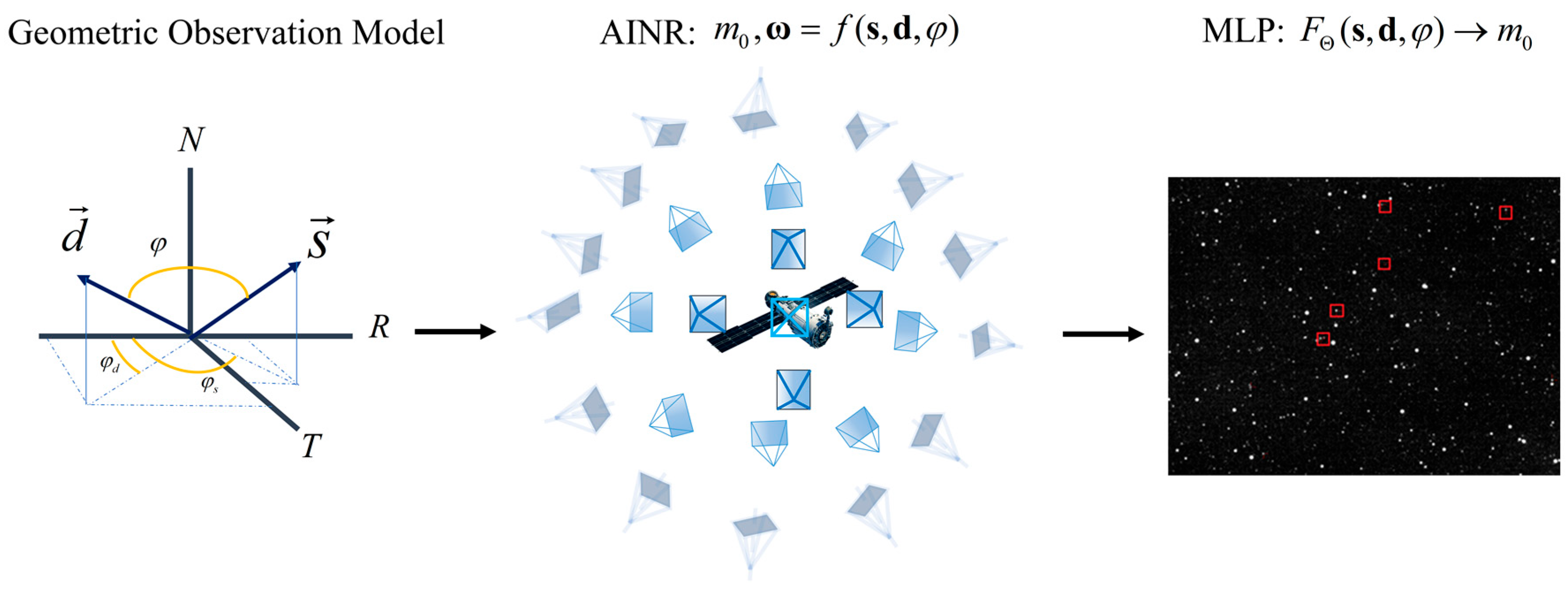
To synthesize the photometric and geometric relationships from every light direction, this paper primarily establishes a mapping relationship using implicit neural functions for spatial geometric and photometric transformations. This process is accomplished by systematically querying the spatial solid angles ω and apparent magnitude m 0 , in conjunction with the spatial positions, within the observation geometric model across specific radiation directions. This methodology enables the creation of comprehensive representations of the optical scattering characteristics of spatial objects from arbitrary light divergence directions and supports the detailed analysis of the satellite’s surface structure and properties, as illustrated in Figure 2.
In astronomy, the equivalent apparent magnitude is frequently employed to characterize the optical scattering properties of space objects [18]. The illumination conditions for these objects are distinctively unique, with the Sun serving as their only light source. The scattered light from an object enters the detector’s field of view, allowing the detector to measure the brightness of both the target and a standard star. Given the known brightness of the standard star, the brightness data of the space object can subsequently be derived. The target’s magnitude is inherently linked to factors such as the type of surface material, shape structure, size of the object, the direction of sunlight incidence, and the direction of observational reception, thus reflecting the intrinsic scattering characteristics of the target [19]. Therefore, for optical observations of space objects, the brightness is typically quantified in terms of magnitude [20].
The equivalent apparent magnitude is measured in illuminance units. Internationally, it is stipulated that an illuminance value of a space object with a magnitude of 0 is E 1 = 2 . 65 × 10 - 6 lx [21]. When the irradiance ratio between two celestial bodies is 100, the difference between their apparent magnitudes is 5, as articulated by the following formula:
E 2 E 1 = 100 ( m 1 m 2 ) / 5 = 2.512 m 1 m 2
where m 1 and m 2 represent the equivalent apparent magnitudes of the celestial bodies, and E 1 and E 2 denote their corresponding illuminance values.
When the distance between the target satellite and the detector is significantly greater than the aperture diameter of the detector, the detector’s aperture is effectively modeled as a plane perpendicular to the observation direction. In the case of point target detection, the light that is reflected off the target and subsequently enters the aperture is presumed to be parallel. This assumption leads to a uniform distribution of irradiance across the aperture surface [22]. Assuming K 0 is the average luminous efficacy within the wavelength range, then in the 0.45~0.90 μm band, K 0 is approximately 158 l m / W [23]. Therefore, the relationship between the satellite’s irradiance E m and its magnitude m at the detector’s aperture is established as follows:
m = 13.98 2.5 lg ( E m K 0 )
In this paper, the distance is uniformly normalized to 300 km to simplify calculations. The focus is solely on the relationship between the change in angular data characteristics and the surface magnitude of the space target. Let R c represent the distance between the satellite and the measurement station (in kilometers), which is then converted to the normalized standard distance for calculation. Let m r e f denote the equivalent luminance measurement value. Based on these definitions, we derive the following formula:
m r e f = m + 5 log ( 300 R c )
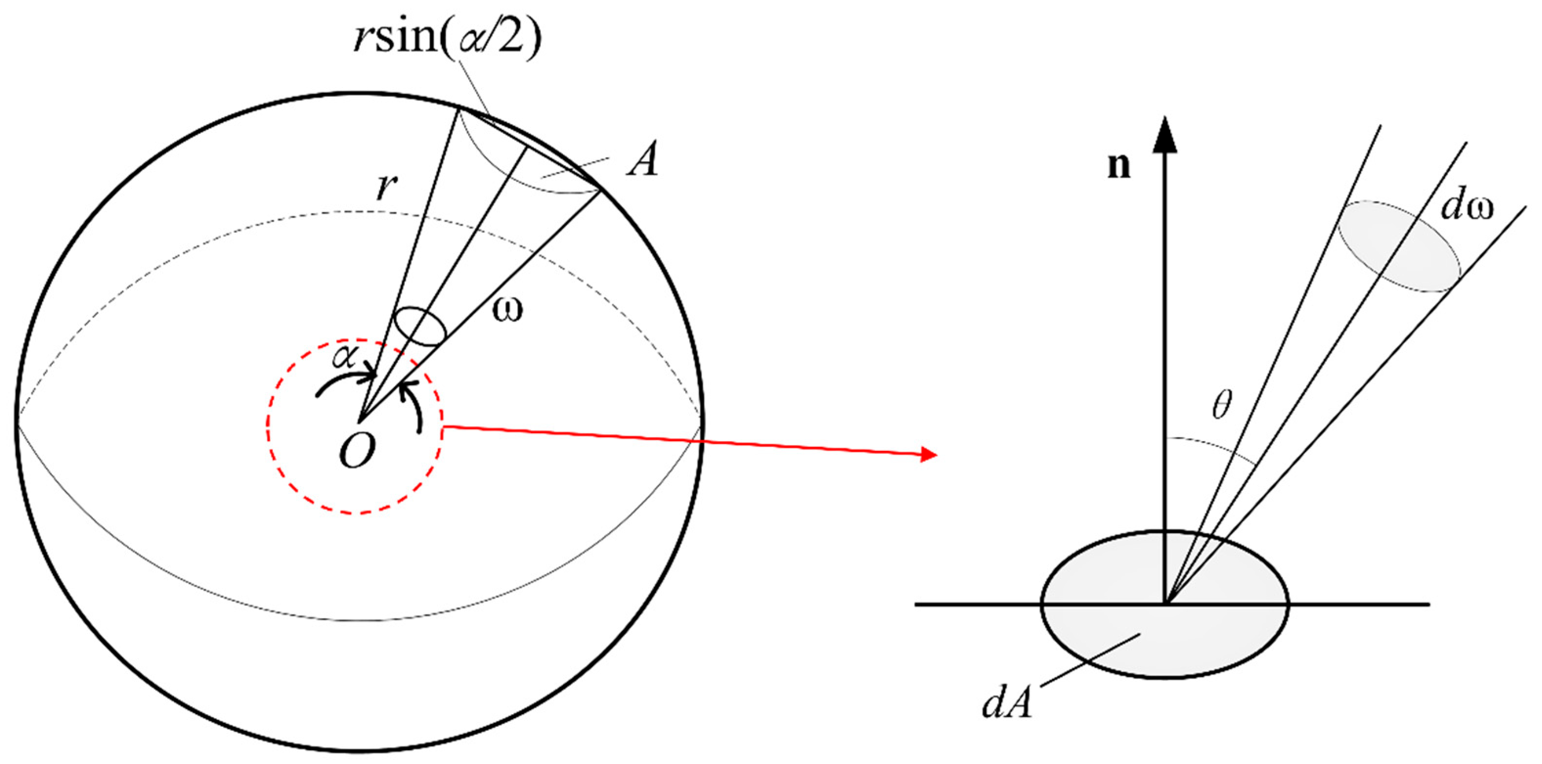
The ratio of the area on the sphere A to the radius of the ball r squared is the solid angle ω in degrees of the sphere. 1 S r is equal to the solid angle when the surface area of the sphere is r 2 , so the solid angle subtended by the entire sphere at its center is 4 π S r . As illustrated in Figure 3, for very small solid angles, the area of the base of a cone can be approximated instead of the sphere for calculation.
ω = 1 4 π α 2
The solid angle ω is a measure of three-dimensional angular extents, while the surface element A quantifies three-dimensional surface areas. The relationship between these two measures can be articulated through the concept of projection.
d ω = d A cos θ r 2
Radiance L 0 refers to the ratio of the radiative intensity emitted by a surface element (including that point) in the direction of observation to the orthogonal projection area of the surface element on a plane perpendicular to the direction of observation.
L 0 = d 2 Φ d ω d A cos θ
where d ω represents the solid angle element; θ is the angle between the surface normal and the direction of radiation; d A denotes the radiation source surface element; and Φ is the radiant flux, which refers to the power to emit, propagate, or receive energy by means of radiation.
When the Sun, the object, and the measurement station need to meet the observation geometric constraints in Section 2.1.3, an analysis model for the optical scattering characteristics of space targets. This model is developed using Equation (10) and incorporates the classical definition of the spectral Bidirectional Reflectance Distribution Function (BRDF) for space targets based on enhanced implicit neural representation techniques [24].
m = 4 π A E m f ( s ^ R , s ^ T , s ^ N , d ^ R , d ^ T , d ^ N ) cos φ s cos φ d d ( F Θ ( L d , ( ω , t ) ) )
It is worth noting that the absorption and scattering of light by gas molecules and small particles in the Earth’s atmosphere frequently result in reduced illuminance. The classical formula for the atmospheric refractive index, derived under ideal conditions, often proves challenging to apply accurately in the actual space environment [25]. The model proposed in this paper employs nested functions and corrections based on empirical data to mitigate error accumulation due to atmospheric extinction.
Given a spatial corner element of ω , in the short distance d t , denoted as follows:
L d L s = d L d = ω L s d t
If the light travels a distance t , the remainder is expressed as follows:
T ( t ) = exp ( 0 t ω d t )
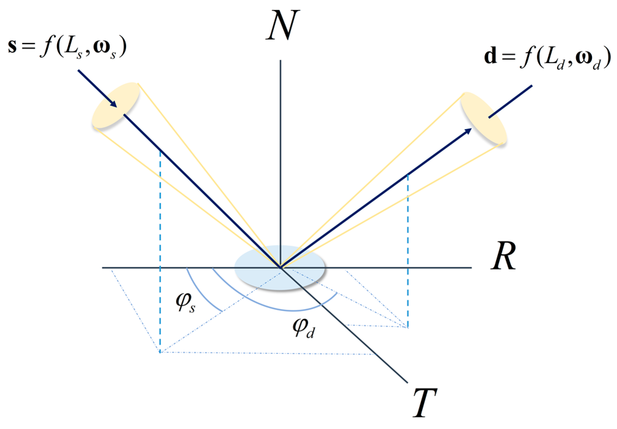
Figure 4 illustrates the process of ray geometry transformations. Therefore, by integrating the radiance at a position p ( t ) = o + d t along the viewing ray d from the near plane to the far plane within the view frustum, the radiance at distance o can be estimated.
C ( o , d ) = t n e a r t f a r R ( t ) ω ( p ( t ) ) L d ( p ( t ) ) d t
The numerical integration after the expansion of the above equation is as follows:
C ^ = i = 0 N T i α i l i , where T i = exp ( i = 1 i 1 ω i δ i ) α i = 1 exp ( ω i δ i ) δ i = t i + 1 t i
l i and ω i can be derived by successive integration of the function f ( o + d ( t i ) , d ) . During the training process, each piece of positional information corresponds to a specific set of luminance data, with the aim of minimizing the reconstruction loss between the luminance values predicted through the model and the true value. All arbitrary directions in the space that satisfy the optical geometric constraints and remain unobstructed are differentiable. Due to the anisotropy of optical materials, scattering characteristics vary with direction, a phenomenon that is particularly pronounced in mirror-reflecting materials. Consequently, in the context of AINRs, a unique mapping relationship exists between the input and output. This unique relationship is leveraged by jointly optimizing the implicit neural representation and its parameters through the minimization of reconstruction loss. The method can effectively predict the luminance information in complex 3D space with minimal input information [26].

2.2.2. Structure of MLP

The nine-layer MLP network architecture employed in this paper is illustrated in Figure 5. This architecture comprises fully connected layers, activation layers, and batch normalization layers, among others. The network F Θ ( s , d , φ ) m 0 is utilized to approximate the continuous 7D spatial optical scattering characteristics and optimize its weights Θ, enabling it to map the input 7D spatial parameters to their corresponding magnitude values and omnidirectional view directions, thus achieving predictions at the physical level.
Compared with traditional neural networks, which primarily derive outputs through inference or prediction, the MLP in this study adopts a more nuanced approach. It implicitly learns the 3D spatial optical properties by fitting and memorizing the relative position data, viewing angles, and radiation field distributions encountered in the training set. Consequently, it consistently generates updates to the satellite surface’s scattered luminance as it reacts to changing conditions. Employing an MLP as the underlying structure of neural radiation ensures the precise capture of complex, nonlinear relationships inherent in the data and maintains the system’s computational efficiency and simplicity. This methodological choice optimizes both performance and manageability [27].
The architecture begins with an input layer designed to receive seven-dimensional angle data { s x , s y , s z , d x , d y , d z , φ } mapped by the neural implicit function. The network’s first fully connected layer contains 2048 neurons optimized for handling the volume of input samples. Subsequently, the second fully connected layer comprises 1024 neurons. These layers aggregate features and engage in training to learn and perform a reasoned mapping to higher-level features as required by the network’s architecture. Both activation layers use the tanh function, as specified in Equation (22). This function is symmetric about the origin, promoting faster convergence rates and effectively compressing the input to the interval (−1, 1). Such characteristics align well with the distribution traits of the normalized, preprocessed photometric sequence data, enabling the capture of complex, nonlinear relationships between the data points, thereby enhancing prediction accuracy. The batch normalization layer standardizes the inputs for each batch by setting all mini-batch sizes to 2048. This normalization maintains the stability of the distribution across batches, mitigates covariate shifts, and enhances the overall stability and efficiency of the training process. The final layer is a regression layer that outputs one-dimensional photometric data, utilizing neural implicit representation to continuously integrate the model’s predictions.
tanh ( x ) = e x e x e x + e x
In order to prevent overfitting, a dropout mechanism with a rate of 0.3 is incorporated into the two fully connected layers. This mechanism irregularly deactivates neurons in a specified proportion during each training session, effectively reducing the risk of overfitting by diminishing the synergistic effects of certain features. Functioning akin to an ensemble method, where each training session randomly alters the model structure due to dropout, multiple training sessions cumulatively resemble the averaging effect of multiple models. This approach significantly enhances the model’s generalization capabilities while concurrently addressing overfitting concerns.
The implicit neural representation model excels in capturing subtle patterns and complex relationships in the input data through adaptive memory learning and nonlinear transformations. This model is particularly adept at handling challenges associated with the optical characterization of spatial objects, which typically involve intricate high-dimensional spatial 3D data and nonlinear mapping relationships. Through its training process, the model autonomously learns these complex mappings, thereby facilitating precise analysis of the optical properties of spatial objects without the need for explicit programming directives.

2.2.3. Reconstructing the Loss Function

In designing the loss function, the output of the model is conceptualized as the radiance reflected from the surface of the satellite, while the phase angle is recognized for its periodic nature within the time-series photometric data obtained from omnidirectional angular simulations. In order to ensure the sensitivity of the model to this periodicity feature and to incorporate the physical significance inherent in the problem’s nature, a reconstructed loss function is proposed. This function not only effectively calculates the discrepancy between predicted and actual values but also robustly accounts for the periodicity of the phase angle.
The standard approach to training a neural network model involves minimizing the empirical loss between the model’s predicted value Y ^ i relative to the known true value Y i across all i samples in the training dataset where i [ 1 , N s ] . First, the Mean Square Error (MSE) is used as the fundamental term of the loss function, aiming to minimize the MSE between the actual values and the predictions made by the model.
L M S E ( Y i ; Y ^ i ) = 1 N s i = 1 N ( Δ ( Y i , Y ^ i ) ) 2
N s represents the number of samples; Δ is a difference operator that describes the variations among discrete variables. Analogous to a differential operator in continuous variables, capturing small variations in model predictions more efficiently, thereby improving computational stability.
Overall, incorporating physical factors into the consideration of the loss function ensures that the iterative convergence of the model parameters is influenced not only by the descending gradient of the MSE equation but also by constraints imposed by the physical nature of the problem. Since the unit-discretization vectors for the six angles exclusively indicate direction without magnitude, a periodic loss term is introduced to quantitatively describe the physical relationship between the periodically varying phase angles φ and the model predictions.
L P H Y ( φ j , C ^ j ) = ( 1 N ) j = 1 N s sin 2 ( 2 π P | Δ C j | )
The fit optimization metric is based on the known geometric constraints inherent in the photometric predictions of spatial objects. These constraints incorporate the rate of change of the phase angle and its temporal dynamics. Where subscript j denotes the time-dependent component, [ φ j , C j ] j = 1 N s denotes the set of N s time series, P is the period of the observed quantity phase angle φ , P [ 0 , π ] ; and | Δ C j | denotes the absolute error between the predicted and the true value of the radiant brightness at progressively smaller distances along the direction of the incoming pupil’s optic rays.
The comprehensive neural network learning objective outlined in this paper contains both loss functions in the following form.
L = L M S E ( Y i ; Y ^ i ) + λ L P H Y ( φ j , C ^ j )
λ is a hyperparameter that modulates the relative importance of the two loss terms, integrating the significance of well-established physical information alongside the empirical loss function typically found in “black box” approaches. Thus, Equation (25) allows the trained model to capture the advantages of the “black box” neural network approach while regularizing the MLP network. This configuration enables the model to prioritize learning the features that are most pivotal for accurate prediction.

3. Modeling System Approach

3.1. Pre-Training Models Based on TL

In practical training, two common challenges are frequently encountered: first, training without prior knowledge may yield accurate test results in isolated instances but requires a disproportionately high number of inputs to achieve convergence; second, the exploitation of inherent biases in the data can appear to accelerate learning superficially, yet this often results in compromised generalization capabilities.
Transfer Learning (TL) is a machine learning method that is designed to transfer knowledge learned from one task to another related task. It is particularly beneficial in scenarios characterized by data scarcity, annotation difficulties or domain changes. The primary objective of TL is to enhance both the performance and generalization capabilities of models by leveraging knowledge from the source domain to facilitate learning in the target domain. This approach aims to expedite model convergence, augment generalization abilities, or adapt to tasks in new domains [28].
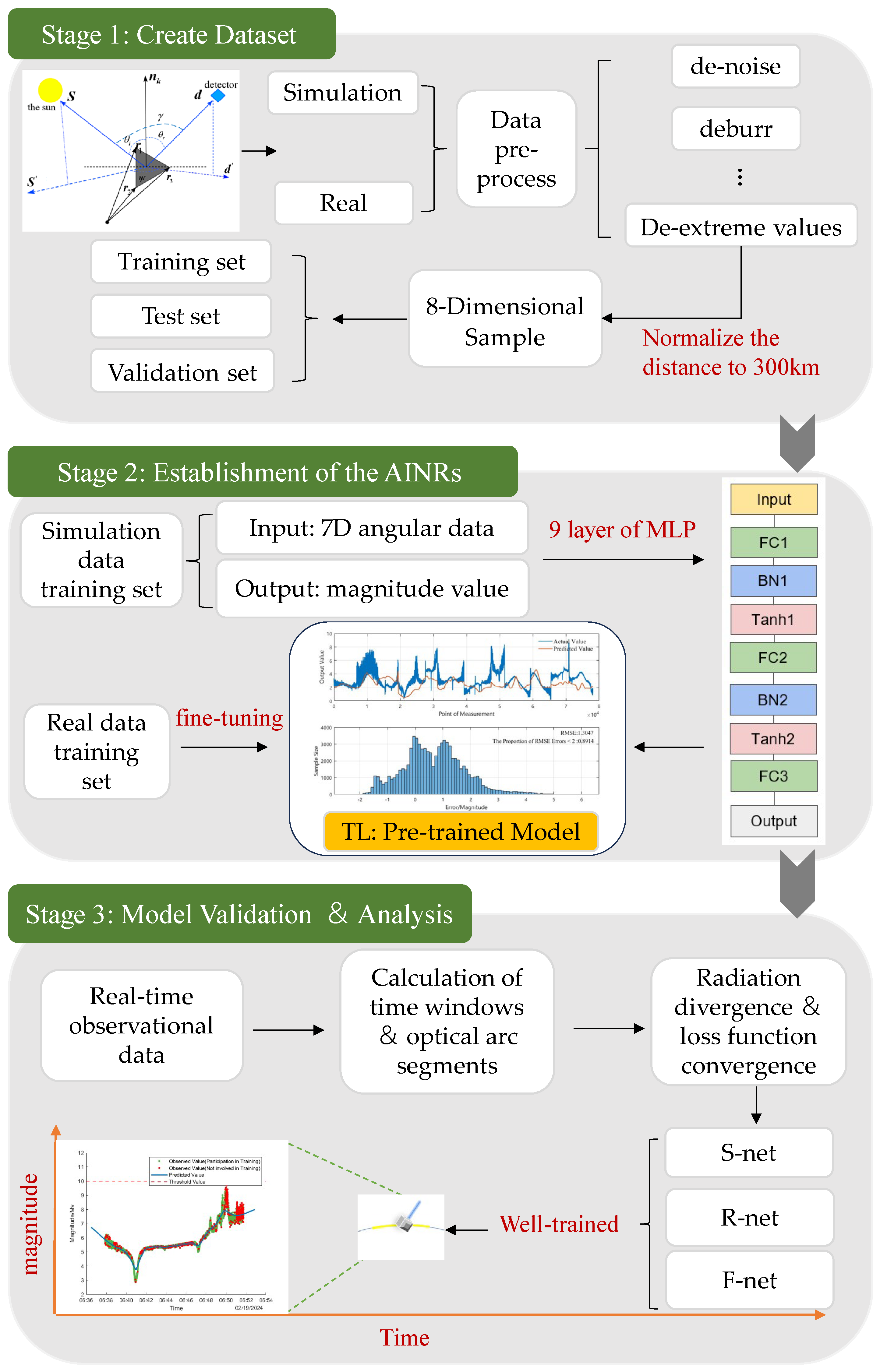
In this paper, a pre-training model based on TL is introduced, with the engineering process and modeling system framework illustrated in Figure 6. Stage 1 involves creating a dataset, establishing the observation geometry model of the “Sun–Satellite–Station”, preprocessing the photometric raw observation data and normalizing the distance to 300 km to form the training set, testing set, and validation set. Stage 2 combines the aforementioned coordinate system conversion and astronomical observational theory to establish a photometric prediction model based on AINRs. This stage includes hyper-parameter tuning to find the optimal 9-layer MLP based on the TL theory, and the introduction of real data to fine-tune the pre-trained model’s parameters. The form of the reconstructed loss function manifests itself as a combination of data-driven and physically driven model alignment, ensuring that the convergence of the loss function accuracy, descent gradient, and weight adjustment meet the requirements of the actual dual problem context. Stage 3 involves model validation and analysis, including selecting satellite types based on real-time observations and using the corresponding AINR models trained through TL. This stage integrates prior orbital information to calculate optically visible arc segments within future time windows, then successively obtains the corresponding photometric prediction values of the satellite surfaces based on neural radiance fields from any orientation in three-dimensional space. Finally, the prediction accuracies of the models trained under three different data combination modes are compared.
We established a multilayer functional relationship through AINRs, mapping the seven-dimensional angular data input in the RTN coordinate system to a one-dimensional apparent magnitude output. In this framework, the combination of data-driven and physics-driven model registration is achieved through the form of a reconstruction loss function. The design of this implicit neural representation adheres to the fundamental physical principles of the inverse problem, enabling the construction of a network with enhanced generalization capabilities compared to methods that rely solely on data-driven or entirely simulation-based.

3.2. Construction of Datasets

To verify the predictive accuracy of the proposed method, we utilized a combination of simulated and real photometric observation data. The raw data were categorized into omnidirectional angular simulation data and ground station measured data. The time-series photometric signals obtained from the ground-based observation system are influenced by various factors, including the position of the space target relative to the Sun and the ground-based observation system. Additionally, these signals encapsulate critical characteristic parameters such as the space object’s orbit, attitude, and mass, which are essential for accurate modeling.
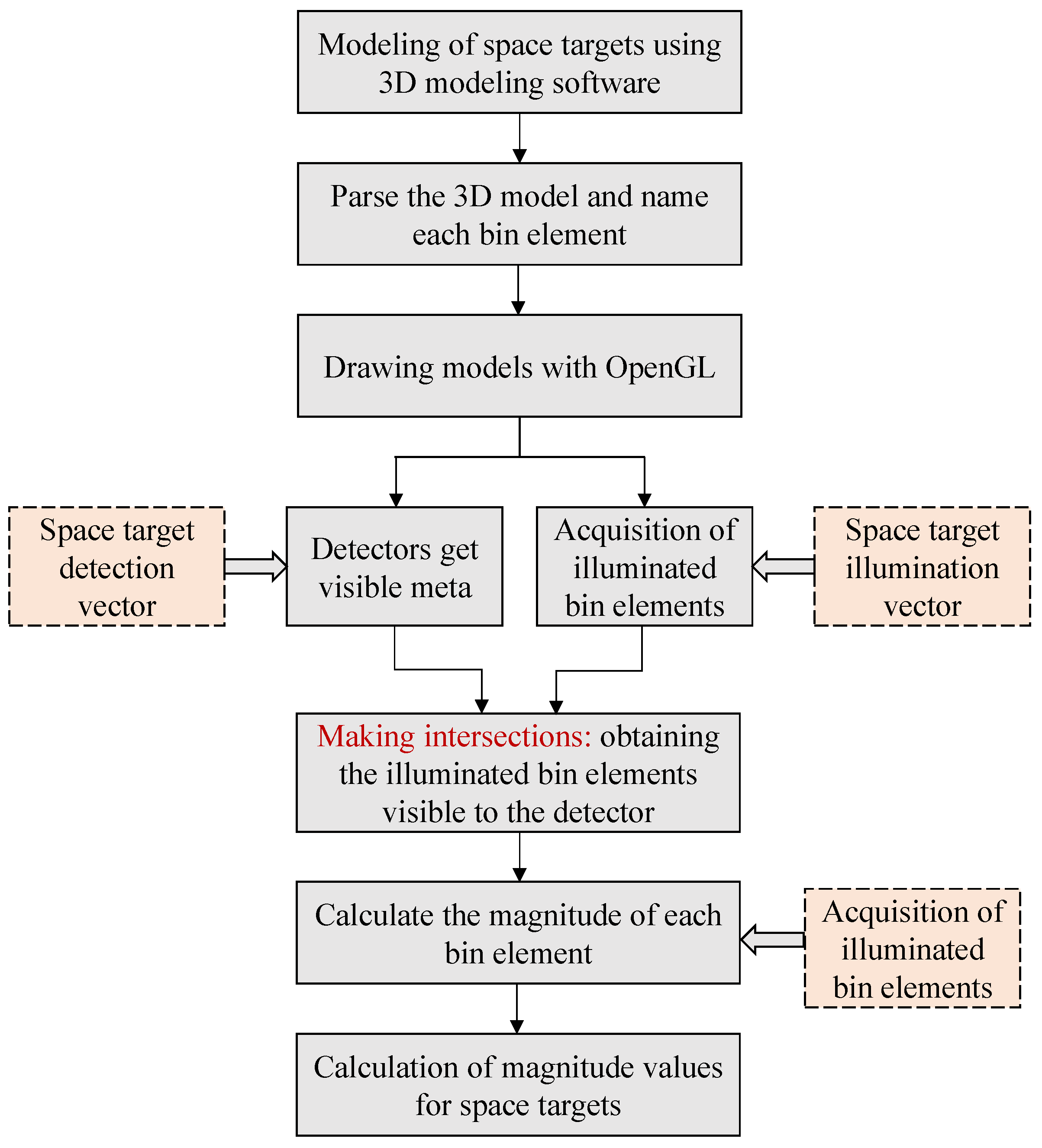
  • The omnidirectional angle simulation data was generated from the ground-based optical observation simulation software. This data are crucial for analyzing the fundamental principle and numerical simulation process of the brightness of the optical scattering characteristics, as depicted in Figure 7, which illustrates the flowchart of the omnidirectional angle simulation software algorithm designed by our research team [29]. The primary steps in generating this data include constructing a three-dimensional model of the object based on the space object image acquired by optical telescope or high-resolution radar; determining the angular information corresponding to each face element of the space object under the orbital coordinate system; applying the actual BRDF model to components such as the sailplane, antenna, and other components, while other components are modeled based on the Lambertian body material, automatically optimizing and adjusting the object’s altitude, components, and the reflectivity of different face elements to compute object brightness; iteratively adjusting the above variables based on the prediction results until the error meets specified requirements [30].
  • The experimental dataset originates from the Small Optoelectronic Innovation Practice Platform at the Space Engineering University. This platform is equipped to automatically interface with site meteorological monitoring equipment and operates in a preset multitasking mode, achieving unmanned equipment operation and data acquisition. The telescope utilized is a high-performance telescope with a 150 mm aperture (f/200) [31], positioned at geographical coordinates 116°40′4.79″E longitude, 40°21′22.36″N latitude, and an altitude of 87.41 m. To ensure the effectiveness of the satellite’s surface photometric characteristic inversion, the data are primarily derived from long-term observations of a three-axis stabilized artificial satellite by a single ground station, with the distance between the station and the satellite normalized to 300 km. The data produced by the platform also provide the potential for a myriad of other future research topics in space situational awareness, such as attitude control, and the platform will continue to drive research for years to come.
In this paper, the training dataset is utilized as a cross-validation set with a designated ratio of 80%, while the test dataset serves as a blind set with a set ratio of 20%. This configuration enhances the implicit neural representation model’s ability to generalize to new data by simulating novel and previously unseen data prediction scenarios. This approach deliberately avoids bias in the data and establishes an MLP mechanism with robust generalization capabilities. Additionally, the model employs early stopping techniques to ensure optimal convergence of the model’s weights rather than extending training across all epochs.

3.3. Evaluation Indicators

1.
Root Mean Square Error (RMSE);
RMSE serves as a typical metric for regression models, quantifying the sample standard deviation of the differences (residuals) between predicted and observed values. This metric effectively captures these residuals within the dataset. In the context of nonlinear fitting problems, a smaller RMSE indicates a better fit.
R M S E = 1 n i = 1 n ( y i y ^ i ) 2 [ 0 , + )
2.
Mean Absolute Error (MAE);
MAE is utilized to measure the average absolute error between predicted values and actual values. This metric represents a linear score that is in a non-negative format, ensuring that each individual discrepancy is treated with equal importance in the mean calculation. A smaller MAE value is indicative of a more accurate model fit.
M A E = 1 n i = 1 n | y i y ^ i | [ 0 , + )

4. Performance Evaluation

4.1. Input Parameters

In the early stage of the project, we contemplated utilizing four angles as inputs: the azimuth and elevation obtained by decomposing s and d in the RTN coordinate system. For a detailed definition of this coordinate system, please refer to Section 2.1.1. The azimuth angle is defined as the angle between the projection of the vector onto the XY plane and the X-axis, with a positive direction towards the Y-axis. The elevation angle is defined as the angle between the vector and the XY plane, with the positive direction towards the Z-axis.
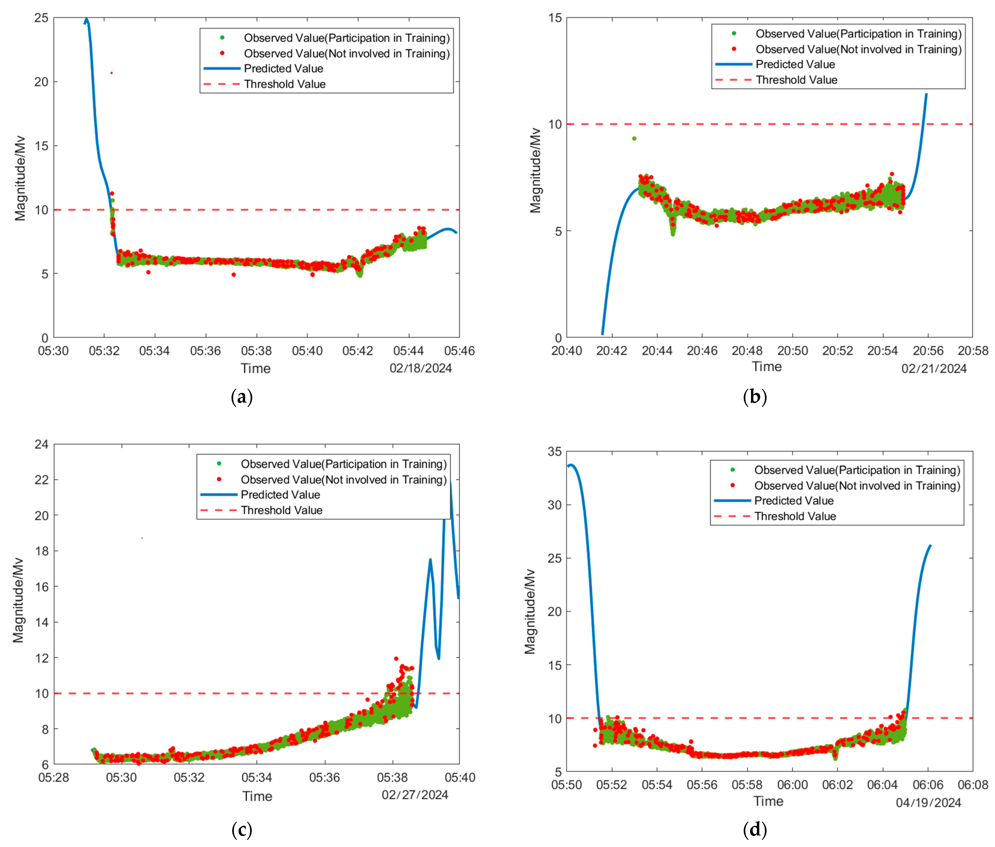
During the phase where only angle data was used as predictive input, we encountered several challenges. As illustrated in Figure 8, to swiftly assess the efficacy of the 4-dimensional input configuration, we employed the R−net, which required a minimal amount of sample data volume and computational memory for predictions. We selected random time windows of telescope observation data from 18 February, 21 February, 27 February, and 19 April 2024, respectively. Based on the original dataset, we calculated the specific time periods during which optically visible arc segments were present on these dates and subsequently conducted predictions based on the R−net. The red scatter points represent data that were excluded from the training set, i.e., outliers and spikes that were removed during preprocessing, while the green scatter points represent the data that were retained for training. The red dashed line represents the upper threshold value of the apparent magnitude in the actual application scenarios, and the blue solid line indicates the predicted situation.
Observations of the predictive models have consistently shown that the prediction curves often exhibit anomalous behaviors such as sharp increases, sharp decreases, and oscillations. These phenomena typically manifest at the beginning and end stages of data appearance and disappearance. Such irregularities are primarily attributed to the inherent characteristics of the angular data used in the predictions. Specifically, the periodicity of azimuth, elevation, and phase angles introduces complexities when conducting continuous predictions in three-dimensional space using implicit neural representations. Normalizing nodes during periodic transitions often results in overlapping values for what should be distinct measurement points, as seen in the azimuth angle range from 0° to 360°, where normalization causes the values of the first and last points to coincide, leading to divergences observed as anomalies in the prediction curves.
In response to these findings, this paper adopts a refined approach for handling the angular data. The original four azimuth and elevation angles are converted into unit vectors along the three coordinate axes of the RTN coordinate system, as detailed in Section 2.1.2. Finally, the network utilizes these six decomposed unit vectors along with the phase angle as input parameters, making a total of seven parameters. The phase angle is strategically sampled at 4° on the simulated data set. This approach helps avoid overlapping phenomena and ensures that the integrity and distinctiveness of the angular data are maintained.
Considering the two types of data sources mentioned in Section 3.2, the experimental setup conducted various combinations of simulated and measured data to train, resulting in distinct network models as outlined in Table 1. Specifically, the model trained with omnidirectional angle simulated data is denoted as S−net, while the model trained using data measured by the ground-based telescope is designated R−net. This study primarily employs a preprocessing method that fuses the aforementioned two types of data, namely F−net, as shown in Stage 2 of Figure 6. Initially, the model trained with simulated data is utilized as a foundational pre-trained model for TL. Subsequently, satellite-measured data of different types are methodically used to fine-tune the corresponding pre-trained network. This fine-tuning process involves optimizing parameters such as weights, bias coefficients, the learning rate, batch size, and the decay cycle. The model is then refined to address specific tasks pertinent to the respective satellite series. The various AINR models are archived in a model repository, facilitating convenient access and real-time application for photometric predictions.

4.2. Model Predictions

The three types of models described in Table 1 are validated through a combined pre-trained transfer process. The initial learning rate for the MLP network is set at 0.0001, with a learning rate decay factor of 0.15 and a decay period of 5. The minimum batch size is set to 2048. An L2 regularization term is selected with a regularization coefficient of 0.001, and the training is capped at a maximum of 100 epochs. The prediction results are as follows:
1.
S−net
As depicted in Figure 9, the performance of the S−net prediction is illustrated. Four days were randomly selected for optical arc segment prediction: 18 February, 19 February, 21 February 2024, and 19 April 2024. During these periods of continuous visibility, the ample simulation data ensure that the orientation information in three-dimensional space is relatively consistent, addressing anomalies at the beginning and end of data sequences. However, the model’s ability to predict apparent magnitude shows poor fitting performance, with only a small portion of the data falling within an error range of two magnitudes, and the trend of the fitting curve does not align closely with the actual observations. Furthermore, the model exhibits weak generalization performance on real data test sets it has not previously encountered. This inadequacy hinders the model’s adaptability to variations in the test set and to mitigate the impacts of spatial environmental variations, ground measurement inaccuracies, and other practical challenges. Consequently, relying solely on simulation data from all angles for training proves insufficient.
2.
R−net
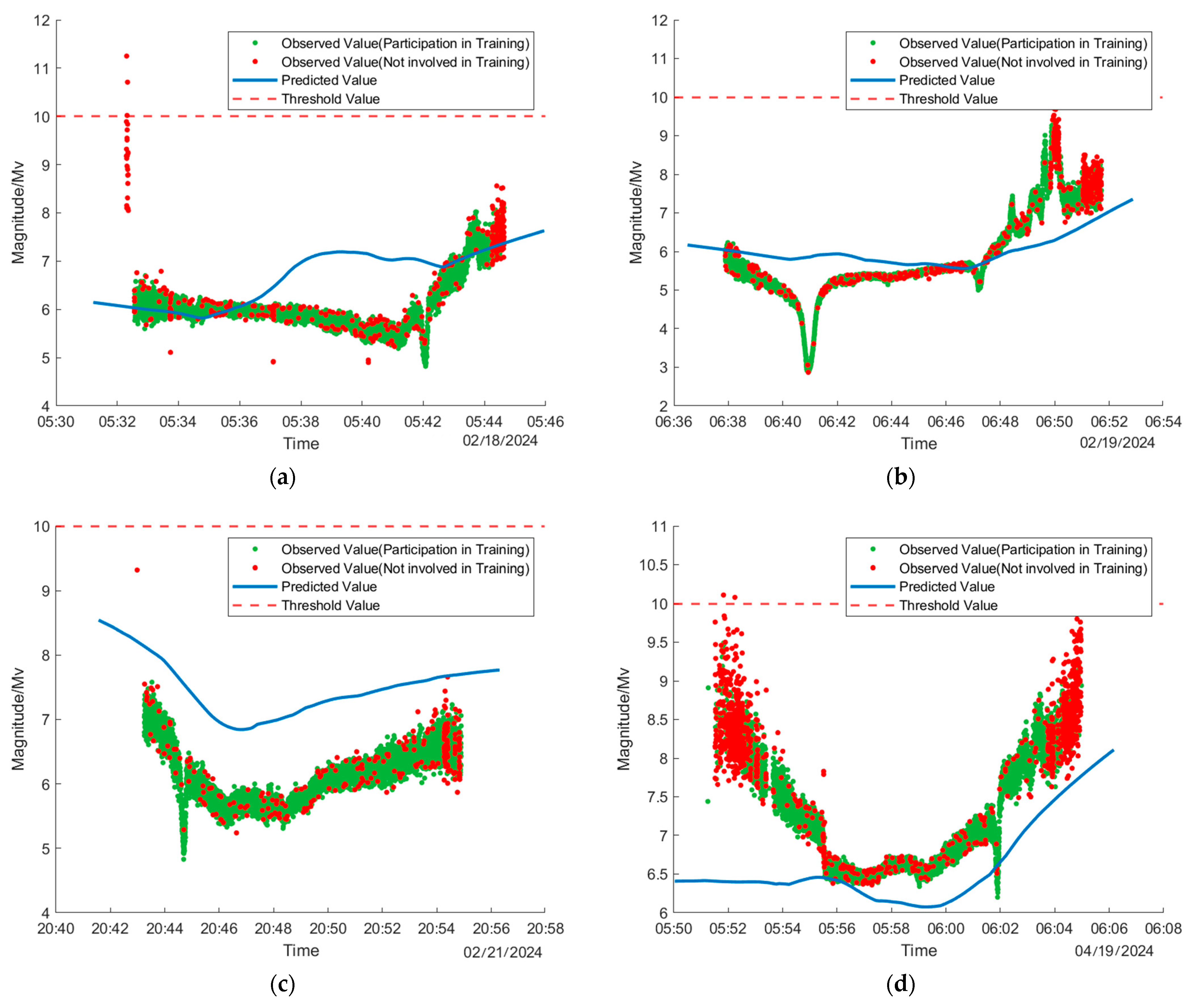
As depicted in Figure 10, the prediction performance of the R−net is presented. Four days were randomly selected for optical arc segment prediction: 18 February, 19 February, 21 February, and 19 April 2024. During these periods of continuous visibility, the model demonstrates moderate fitting performance in predicting apparent magnitude, and the trend of the fitting curve generally aligns with the changes observed in the test set. However, the model encounters difficulties in achieving low absolute errors in apparent magnitude, and it struggles to accurately predict transient phenomena such as the “flash” effect that occurs between 06:40 and 06:42, as shown in (b) effectively. While the model trained based on the measured data exhibits proficiency in trend approximation, the associated errors fall short of the standards required for practical engineering applications. Therefore, relying exclusively on measured data for model training proves inadequate.
3.
F−net
As illustrated in Figure 11, the prediction performance of the F−net is presented. Four days were randomly selected for optical arc segment prediction: 18 February 2024, 19 February 2024, 21 February 2024, and 19 April 2024. Within the continuous visibility period, the model demonstrates a robust fitting performance in predicting apparent magnitude. The predicted trend of the fitting curve not only aligns closely with the variations in the test set but also keeps the error in apparent magnitude within the acceptable limits for engineering purposes. All predicted values meet the requirements of the upper threshold, effectively predicting the “flash” effect that occurs between 06:40 and 06:42, as shown in (b). This achievement incorporates the identification of the material properties of the spatial object and reaches a component-level analysis standard. The experiment validates the effectiveness of the training method that combines simulation data from all angles with measured data, indicating that the pre-training process based on transfer learning and the model based on enhanced implicit neural representations proposed in this paper exhibit potential in the analysis of optical characteristics of space objects. These models are poised for further application in practical engineering contexts.

4.3. Comparison of Results

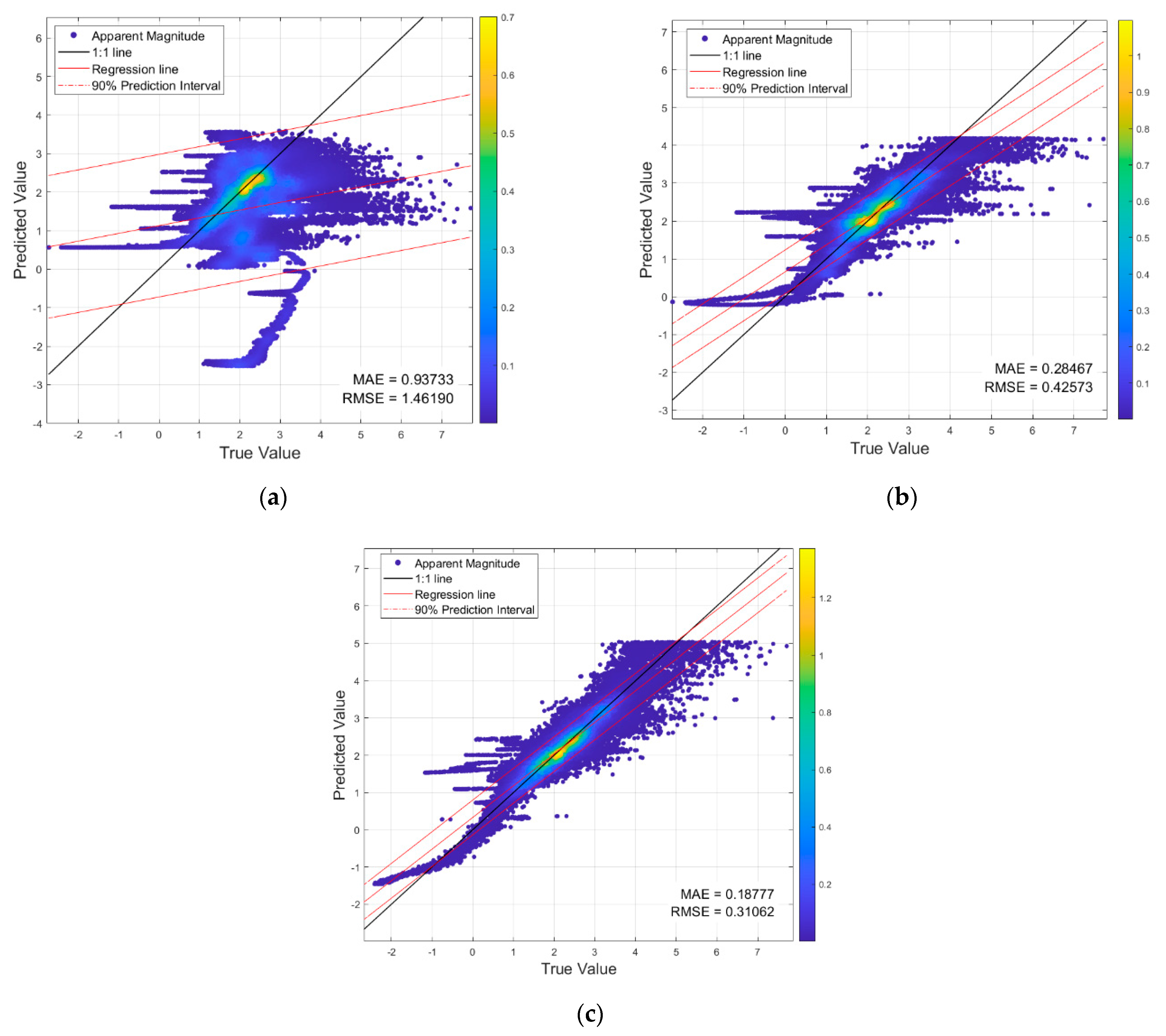
The fitted curves above roughly describe the trend and range of the prediction errors. However, a quantitative analysis has yet to be conducted. For the prediction performance of the three models mentioned, scatter plots accompanied by kernel density estimates are depicted in Figure 12. The non-parametric statistical method of kernel density estimation (KDE) was used, with a Gaussian kernel function as the smoothing mechanism to facilitate a detailed quantitative analysis of the errors using numerical methods [32].
The x−axis represents the actual magnitudes, while the y−axis denotes the magnitudes predicted by the neural network. The 1:1 line, which is the diagonal bisector, is used to assess the fitting performance. When the scatter points lie on this line, it indicates zero fitting error; the further the points deviate from the 1:1 line, the poorer the fitting performance. The right-side label bar displays the probability density estimates, where the color intensity represents different density levels. Areas with colors closer to yellow indicate higher data point density and vice versa. The regression line, fit using the Least Squares Method, illustrates the linear relationship between the independent and dependent variables. The 90% Confidence Interval represents a range that indicates a 90% probability that the true predicted value falls within this interval based on multiple sample experiments. This metric provides a robust estimate of the prediction value’s reliability.
As demonstrated in Figure 12, the F−net demonstrates the most accurate prediction performance, with the regression line’s coefficient approaching the ideal 1:1 line more closely than other models. Moreover, the majority of sample points exhibiting minimal error are densely clustered within the 90% Confidence Interval, underscoring a high level of reliability. As shown in the data analysis in Table 2, the RMSE of F−net is 0.31062, reflecting a significant reduction of 78.75% compared to S−net; similarly, the MAE of F−net is 0.18777, marking a reduction of 79.97% relative to S−net.
The considerable reduction in error percentages underscores the efficacy of the F−net approach when modeling the complex 7D spatial optical scattering characteristics, such as F Θ ( s , d , φ ) m 0 using an MLP network. The weight parameters Θ within the loss function’s gradient descent algorithm have reached optimal values, ensuring that the average absolute error remains well within 0.2 m V Such precision not only meets but exceeds the stringent demands of practical engineering applications and suggests significant potential for broader implementation.

5. Conclusions

Building upon existing methodologies for analyzing spatial object characteristics and integrating features from optical telescope observation data, this paper proposes a spatial object optical characteristic analysis model employing an enhanced implicit neural expression. Starting from the perspective of engineering applications, the model harnesses both raw observational data from ground-based telescopes and simulated data obtained through optical characteristic simulation software at a phase angle interval of 4°. By employing a pre-training process based on transfer learning tailored for engineering simulations, a series of preprocessing steps are executed to produce seven-dimensional input data, facilitating the continuous prediction of apparent magnitude in three-dimensional space. A comparative analysis of the results is subsequently conducted for evaluation.
The results indicate that the model proposed in this study achieves minimal errors on the series of satellites, satisfying the demands of the engineering context. Through a synergistic approach that merges data-driven and physics-driven methodologies and by leveraging the dual advantages of empirical data and theoretical models, continuous adjustments of appropriate network parameters address the abnormal fitting phenomenon caused by the periodicity of angular data. This approach not only attains an early ideal predictive performance but also simplifies the process design, enabling an end-to-end prediction that more closely aligns with practical engineering requirements. The final absolute error of the prediction is controlled within 0.2 m V , demonstrating the model’s robust generalization ability to real-space data and, to some extent, surmounting the limitations of traditional simulation modeling methods in the analysis of space object optical characteristics. This strategy mitigates the issues associated with error accumulation in geometric modeling and establishes a solid foundation for future component-level identification and analysis of satellite surface optical scattering characteristics. Future work will focus on further validating the effectiveness of this model across a broader range of satellite series and conducting routine object surveillance and anomaly detection.

Author Contributions

Conceptualization, Q.Z., X.W. and Y.Z.; methodology, Q.Z., Y.F and X.T.; software, Q.Z.; validation, X.W. and H.T.; formal analysis, Q.Z. and S.Z.; investigation, Q.Z.; resources, C.X., Q.Z. and Y.Z.; writing—original draft preparation, Q.Z., Y.F. and H.T.; writing—review and editing, Q.Z. and X.T.; visualization, Q.Z.; supervision, Y.Z. All authors have read and agreed to the published version of the manuscript.

Funding

This research received no external funding.

Data Availability Statement

The original contributions presented in the study are included in the article, further inquiries can be directed to the corresponding author.

Acknowledgments

We would like to thank everyone who helped with this paper, especially our supervisor and colleagues who made this paper possible.

Conflicts of Interest

The authors declare no conflicts of interest.

Abbreviations

The following abbreviations are used in this manuscript:
AINRsAugmented Implicit Neural Representations
MLPMulti-Layer Perceptron
MAEMean Absolute Error
MSEMean Square Error
RMSERoot Mean Square Error
RTNRadial Transverse Normal
TLTransfer Learning
TLETwo-Line Element

References

  1. Scott, R.L.; Thorsteinson, S.; Abbasi, V. On-Orbit Observations of Conjuncting Space Objects Prior to the Time of Closest Approach. J. Astronaut. Sci. 2020, 67, 1735–1754. [Google Scholar] [CrossRef]
  2. Ruo, M. Research on Key Feature Inversion Method for Space Objects Based on Ground Photometric Signals. Ph.D. Thesis, Harbin Institute of Technology, Harbin, China, 2021. [Google Scholar]
  3. Wang, X.; Huo, Y.; Fang, Y.; Zhang, F.; Wu, Y. ARSRNet: Accurate Space Object Recognition Using Optical Cross Section Curves. Appl. Opt. 2021, 60, 8956. [Google Scholar] [CrossRef] [PubMed]
  4. Friedman, A.M. Observability Analysis for Space Situational Awareness. Ph.D. Thesis, Purdue University, West Lafayette, IN, USA, 2022. [Google Scholar]
  5. Bieron, J.; Peers, P. An Adaptive BRDF Fitting Metric. Comput. Graph. Forum 2020, 39, 59–74. [Google Scholar] [CrossRef]
  6. Zhan, P. BRDF-Based Light Scattering Characterization of Random Rough Surfaces. Ph.D. Thesis, University of Chinese Academy of Sciences, Beijing, China, 2024. [Google Scholar]
  7. Little, B.D. Optical Sensor Tasking Optimization for Space Situational Awareness. Ph.D. Thesis, Purdue University, West Lafayette, IN, USA, 2019. [Google Scholar]
  8. Rao, C.; Zhong, L.; Guo, Y.; Li, M.; Zhang, L.; Wei, K. Astronomical Adaptive Optics: A Review. PhotoniX 2024, 5, 16. [Google Scholar] [CrossRef]
  9. Liu, X.; Wu, J.; Man, Y.; Xu, X.; Guo, J. Multi-Objective Recognition Based on Deep Learning. Aircr. Eng. Aerosp. Technol. 2020, 92, 1185–1193. [Google Scholar] [CrossRef]
  10. Kerr, E.; Petersen, E.G.; Talon, P.; Petit, D.; Dorn, C.; Eves, S. Using AI to Analyze Light Curves for GEO Object Characterization. In Proceedings of the 22nd Advanced Maui Optical and Space Surveillance Technologies Conference (AMOS), Maui, HI, USA, 19–22 September 2021. [Google Scholar]
  11. Singh, N.; Brannum, J.; Ferris, A.; Horwood, J.; Borowski, H.; Aristoff, J. An Automated Indications and Warning System for Enhanced Space Domain Awareness. In Proceedings of the Advanced Maui Optical and Space Surveillance Technologies Conference (AMOS), Maui, HI, USA, 16–18 September 2020. [Google Scholar]
  12. Dupree, W.; Penafiel, L.; Gemmer, T. Time Forecasting Satellite Light Curve Patterns Using Neural Networks. In Proceedings of the 22nd Advanced Maui Optical and Space Surveillance Technologies Conference (AMOS), Maui, HI, USA, 19–22 September 2021. [Google Scholar]
  13. Li, H. Space Object Optical Characteristic Calculation Model and Method in the Photoelectric Detection Object. Appl. Opt. 2016, 55, 3689. [Google Scholar] [CrossRef] [PubMed]
  14. Campiti, G.; Brunetti, G.; Braun, V.; Di Sciascio, E.; Ciminelli, C. Orbital Kinematics of Conjuncting Objects in Low-Earth Orbit and Opportunities for Autonomous Observations. Acta Astronaut. 2023, 208, 355–366. [Google Scholar] [CrossRef]
  15. Tao, X.; Li, Z.; Xu, C.; Huo, Y.; Zhang, Y. Track-to-Object Association Algorithm Based on TLE Filtering. Adv. Space Res. 2021, 67, 2304–2318. [Google Scholar] [CrossRef]
  16. Friedman, A.M.; Frueh, C. Observability of Light Curve Inversion for Shape and Feature Determination Exemplified by a Case Analysis. J. Astronaut. Sci. 2022, 69, 537–569. [Google Scholar] [CrossRef]
  17. Mildenhall, B.; Srinivasan, P.P.; Tancik, M.; Barron, J.T.; Ramamoorthi, R.; Ng, R. NeRF: Representing Scenes as Neural Radiance Fields for View Synthesis. Commun. ACM 2022, 65, 99–106. [Google Scholar] [CrossRef]
  18. Ford, E.B.; Seager, S.; Turner, E.L. Characterization of Extrasolar Terrestrial Planets from Diurnal Photometric Variability. Nature 2001, 412, 885–887. [Google Scholar] [CrossRef] [PubMed]
  19. Campbell, T.S. Astrometric and Photometric Data Fusion in Machine Learning-Based Characterization of Resident Space Objects. Ph.D. Thesis, University of Arizona, Tucson, AZ, USA, 2023. [Google Scholar]
  20. Cadmus, R.R. The Relationship between Photometric Measurements and Visual Magnitude Estimates for Red Stars. Astron. J. 2021, 161, 75. [Google Scholar] [CrossRef]
  21. Lei, X.; Lao, Z.; Liu, L.; Chen, J.; Wang, L.; Jiang, S.; Li, M. Telescopic Network of Zhulong for Orbit Determination and Prediction of Space Objects. Remote Sens. 2024, 16, 2282. [Google Scholar] [CrossRef]
  22. Chang, K.; Fletcher, J. Learned Satellite Radiometry Modeling from Linear Pass Observations. In Proceedings of the Advanced Maui Optical and Space Surveillance Technologies Conference (AMOS), Maui, HI, USA, 19–22 September 2023. [Google Scholar]
  23. Baron, F.R.; Jefferies, S.M.; Shcherbik, D.V.; Hall, R.; Johns, D.; Hope, D.A. Hyper-Spectral Speckle Imaging of Resolved Objects. In Proceedings of the Advanced Maui Optical and Space Surveillance Technologies Conference (AMOS), Maui, HI, USA, 19–22 September 2023. [Google Scholar]
  24. Lu, Y. Impact of Starlink Constellation on Early LSST: A Photometric Analysis of Satellite Trails with BRDF Model. arXiv 2024, arXiv:2403.11118. [Google Scholar]
  25. Vasylyev, D.; Semenov, A.A.; Vogel, W. Characterization of Free-Space Quantum Channels. In Proceedings of the Quantum Communications and Quantum Imaging XVI, San Diego, CA, USA, 19–23 August 2018; p. 31. [Google Scholar]
  26. Tancik, M. Object and Scene Reconstruction Using Neural Radiance Fields. Ph.D. Thesis, University of California, Berkeley, CA, USA, 2023. [Google Scholar]
  27. Tancik, M.; Srinivasan, P.P.; Mildenhall, B.; Fridovich-Keil, S.; Raghavan, N.; Singhal, U.; Ramamoorthi, R.; Barron, J.T.; Ng, R. Fourier Features Let Networks Learn High Frequency Functions in Low Dimensional Domains. Adv. Neural Inf. Process. Syst. 2020, 33, 7537–7547. [Google Scholar]
  28. Yang, X.; Nan, X.; Song, B. D2N4: A Discriminative Deep Nearest Neighbor Neural Network for Few-Shot Space Target Recognition. IEEE Trans. Geosci. Remote Sens. 2020, 58, 3667–3676. [Google Scholar] [CrossRef]
  29. Peng, L.; Li, Z.; Xu, C.; Fang, Y.; Zhang, F. Research on Space Object’s Materials Multi-Color Photometry Identification Based on the Extreme Learning Machine Algorithm. Spectrosc. Spectr. Anal. 2018, 39, 363–369. [Google Scholar]
  30. Xu, C.; Zhang, Y.; Li, P.; Li, J. Optical cross-sectional area calculation of spatial objects based on OpenGL pickup technique. J. Opt. 2017, 37, 218–227. [Google Scholar]
  31. Machine Vision Series Lenses for Telescopes. Available online: https://www.forecam.com/RicomCnSolutionShow.asp?Cls=%BB%FA%C6%F7%CA%D3%BE%F5%CF%B5%C1%D0%BE%B5%CD%B7 (accessed on 20 January 2024).
  32. Beirlant, J.; Dudewicz, E.J.; Györfi, L.; van der Meulen, E.C. Estimation of Shannon Differential Entropy: An Extensive Comparative Review. Entropy 1997, 19, 220–246. [Google Scholar]
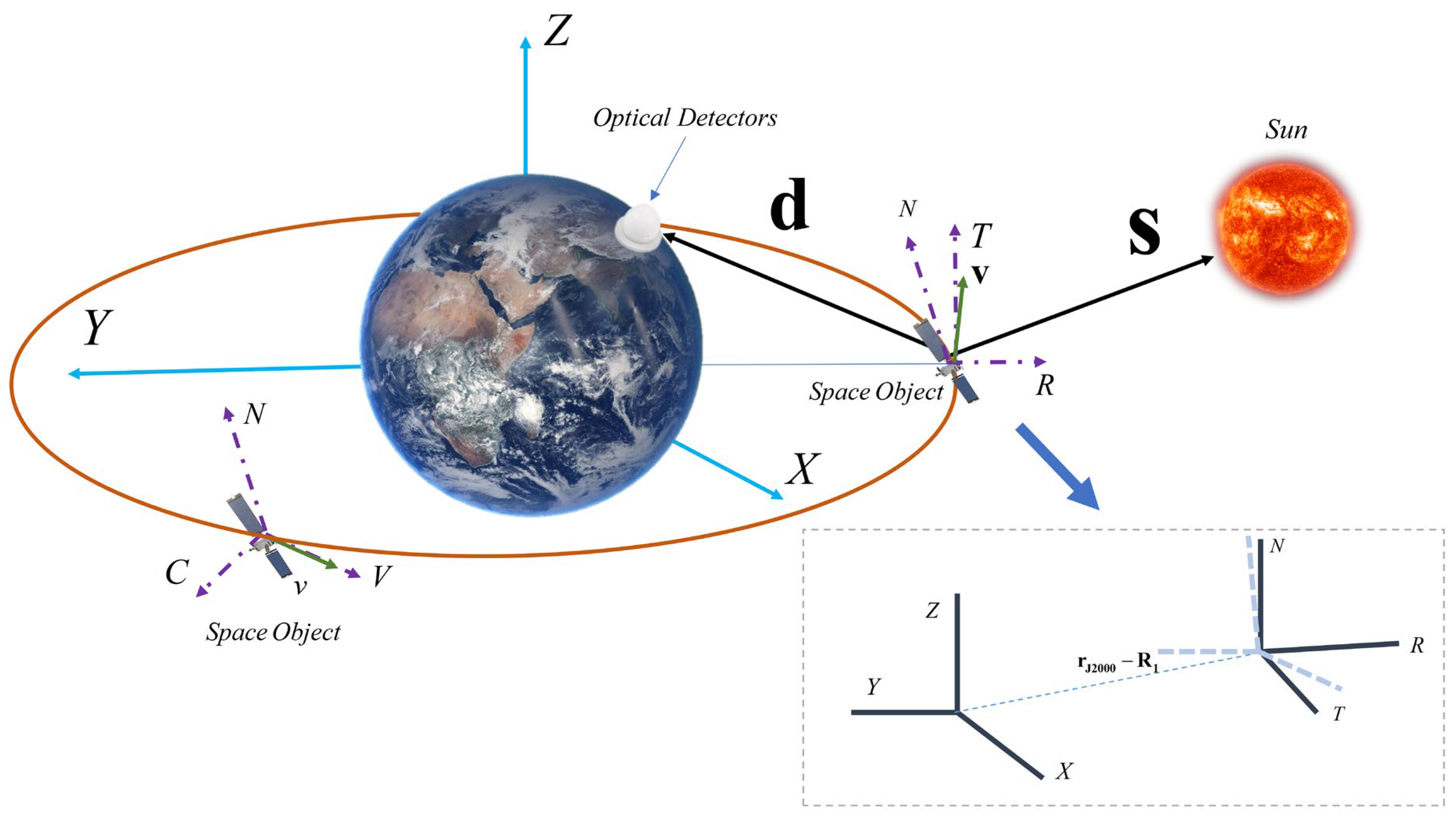
Figure 1. Schematic diagram of the relative geometric relationship and coordinate transformation between the Sun, the satellite, and the probe.
Remotesensing 16 03316 g001
Figure 2. Diagram of the AINRs model and the mapping relationships for geometric and photometric transformations. According to the star maps captured by the ground-based telescope, the red squares indicate the space objects matched using the AINR model.
Remotesensing 16 03316 g002
Figure 3. Diagram of the solid angle and a locally enlarged view showing the relationship between the solid angle and the surface element.
Remotesensing 16 03316 g003
Figure 4. Schematic diagram of the ray geometry transformations and divergence, where p = ( s , d ) is considered as the geometric observation model, ω as the solid angle, L s as the incident radiance, and L d as the reflected radiance.
Remotesensing 16 03316 g004
Figure 5. Schematic diagram of MLP architecture.
Remotesensing 16 03316 g005
Figure 6. Schematic diagram of the pre-training process based on TL and optical scattering characteristics analysis of space objects.
Remotesensing 16 03316 g006
Figure 7. Flowchart of the Algorithmic Process for Photometric Calculations of Complex Space Objects Based on Omnidirectional Angles.
Remotesensing 16 03316 g007
Figure 8. When predicting the curve using only 4D angular data as input, anomalous phenomena such as “jumps” and “sharp increases” may occur. By time information, they can be listed as: (a) 18 February 2024; (b) 21 February 2024; (c) 27 February 2024; (d) 19 April 2024.
Remotesensing 16 03316 g008
Figure 9. S−net model projections across selected dates. The temporal distribution of the data is detailed as follows: (a) 18 February 2024; (b) 19 February 2024; (c) 21 February 2024; (d) 19 April 2024.
Remotesensing 16 03316 g009
Figure 10. R−net model projections across selected dates. The data are presented chronologically as follows: (a) 18 February 2024; (b) 19 February 2024; (c) 21 February 2024; (d) 19 April 2024.
Remotesensing 16 03316 g010
Figure 11. F−net model projections across selected dates. The data are presented chronologically: (a) 18 February 2024; (b) 19 February 2024; (c) 21 February 2024; (d) 19 April 2024.
Remotesensing 16 03316 g011
Figure 12. The KDE scatter plots for the three models. The models are categorized as follows: (a) S−net; (b) R−net; (c) F−net.
Remotesensing 16 03316 g012
Table 1. Network models trained on different types of data, along with descriptions of the models.
NumberNamed ModelDescription
1S−net (Simulation)The network model trained using omnidirectional angle simulated data;
2R−net (Real)The network model trained using ground-based telescope-measured data;
3F−net (Fine-tuned)Utilizing omnidirectional angle simulated data for pretraining the network and continually fine-tuning the network parameters with measured data to obtain the model;
Table 2. Comparison of values of evaluation indicators for a series of satellites.
ModelRMSEPercentage
Reduction
MAEPercentage
Reduction
S−net1.461900.937330
R−net0.425730.70880.284670.6963
F−net0.310620.78750.187770.7997
Disclaimer/Publisher’s Note: The statements, opinions and data contained in all publications are solely those of the individual author(s) and contributor(s) and not of MDPI and/or the editor(s). MDPI and/or the editor(s) disclaim responsibility for any injury to people or property resulting from any ideas, methods, instructions or products referred to in the content.