Characterization of Complex Rock Mass Discontinuities from LiDAR Point Clouds

Abstract

The distribution and development of rock mass discontinuities in 3D space control the deformation and failure characteristics of the rock mass, which in turn affect the strength, permeability, and stability of rock masses. Therefore, it is essential to accurately and efficiently characterize these discontinuities. Light Detection and Ranging (LiDAR) now allows for fast and precise 3D data collection, which supports the creation of new methods for characterizing rock mass discontinuities. However, uneven density distribution and local surface undulations can limit the accuracy of discontinuity characterization. To address this, we propose a method for characterizing complex rock mass discontinuities based on laser point cloud data. This method is capable of processing datasets with varying densities and can reduce over-segmentation in non-planar areas. The suggested approach involves a five-stage process that includes: (1) adaptive resampling of point cloud data based on density comparison; (2) normal vector calculation using Principal Component Analysis (PCA); (3) identifying non-planar areas using a watershed-like algorithm, and determine the main discontinuity sets using Multi-threshold Mean Shift (MTMS); (4) identify single discontinuity clusters using Density-Based Spatial Clustering of Applications with Noise (DBSCAN); (5) fitting discontinuity planes with Random Sample Consensus (RANSAC) and determining discontinuity orientations using analytic geometry. This method was applied to three rock slope datasets and compared with previous research results and manual measurement results. The results indicate that this method can effectively reduce over-segmentation and the characterization results have high accuracy.

1. Introduction

Rock slopes are geological entities with unique structural characteristics, displaying significant discontinuities, heterogeneity, and anisotropy. Due to complex tectonic movements at different historical periods, surface weathering, and stress release processes, rock masses often develop various discontinuities of different scales and properties, such as fractures, joints, bedding planes, and faults. The distribution and evolution of discontinuities in 3D space govern the deformation and failure characteristics of rock masses. It is one of the important factors that affect the strength, permeability, and stability of rock masses [1,2]. The characterization of rock mass discontinuities involves identifying the location, size, and some typical parameters of the discontinuities. Several geometric parameters can quantitatively describe rock discontinuities, such as orientation, roughness, spacing, persistence, and more [3]. Among these, the orientation (dip angle and dip direction) is particularly critical for analyzing the stability of jointed rock masses [4]. For instance, orientation is a critical input parameter in block theory [5], rock mass classification [6], and the use of the limited equilibrium method [7]. Hence, it is extremely important to accurately map these discontinuities and determine the orientation of rock discontinuities in rock engineering [1,8].

Traditionally, geologists use tools such as geological compasses and tape measures to manually measure the discontinuity plane of rock masses using methods like scanline surveys or window sampling to collect their geometric information [9,10]. Although this method is straightforward and user-friendly, it has several significant drawbacks: (1) The measurement process relies entirely on manual execution, which results in low efficiency [11]; (2) The working conditions are easily constrained by terrain and environmental factors [12]; (3) In complex terrains, especially in fragmented rock areas and steep slopes, surveyors may be unable to access specific areas for measurement [13]; (4) Investigators need to have relevant professional backgrounds, and the back of these makes it easy for human errors to occur [14,15]. These limitations constrain the ability to conduct an in-depth analysis of the structural characteristics of rock slopes.

In modern geotechnical engineering and geological exploration, Light Detection and Ranging (LiDAR) and digital photogrammetry are widely used remote sensing techniques for acquiring high-quality 3D point cloud data, capable of capturing high-resolution 3D information [16,17]. The origins of 3D laser scanning technology can be traced back to the mid-20th century. This technology uses 3D laser scanners to rapidly scan and measure target objects, directly capturing the distance, direction, and intensity values of the reflected laser from the object. Due to its ability to collect real-time, high-precision 3D point clouds of rock surfaces without physical contact, this technology eliminates the subjective factors associated with manual contact measurements. Therefore, compared to traditional manual measurement methods, 3D laser scanning offers a more objective and accurate means of data acquisition. These techniques have seen rapid advancement in geological and geotechnical research fields [18]. Rock mass discontinuities can be categorized into planar and linear types. Linear discontinuities primarily manifest as fractures, with their spatial distribution occurring within the rock mass. On the other hand, planar discontinuities are exposed fault surfaces that appear on the rock mass surface after sliding has occurred. This study focuses on the characterization of planar discontinuities. In recent years, many researchers have utilized 3D point cloud data to analyze discontinuities, including discontinuity recognition [19,20,21,22], slope stability analysis [23,24], discontinuity and rapid characterization [25,26]. The widespread use of remote sensing technology in the analysis of rock discontinuities has demonstrated its feasibility and effectiveness.

Currently, the main algorithms used in this field fall into three categories: model fitting, region-growing, and unsupervised clustering. The Random Sample Consensus (RANSAC) algorithm and Randomized Hough Transform (RHT) are two typical model-fitting methods that can detect planes in 3D point clouds. Ge et al. [27] employ the region-growing method to determine the geometric characteristics, including orientation, spacing, and roughness, of rock discontinuities. They perform growth through the differences in normal vectors, thereby obtaining sets of discontinuities with different orientations. The performance of this method is highly dependent on the selection of initial seed points. Unsupervised clustering classifies point clouds based on the similarity of their underlying structure, geometric features, or spatial distribution. Unsupervised clustering methods typically surpass the model-fitting approach in extracting discontinuities from point cloud data, especially when dealing with complex geometries and a wide range of shapes and sizes [22]. K-means [28,29] and its variants [30,31] are common distance-based clustering methods. These methods directly assign groups to each point, which can lead to inaccurate division of boundary points. Slob et al. [32] proposed the automatic identification of discontinuities using fuzzy k-means clustering. This method introduced fuzzy theory and addressed the boundary grouping problem more effectively by calculating membership degrees. However, a significant drawback of such algorithms is the need to preset the number of clusters, making the clustering results highly influenced by subjective factors. To address this issue, scholars have proposed several algorithms that can automatically determine the number of clusters, including the surface classification algorithm [33], improved K-means [34], firefly algorithm [35], unsupervised K-means [36], and optimized K-means [37]. However, partition-based clustering methods, like region-growing techniques, are affected by the choice of initial cluster centers, which affects the clustering results. Density-based clustering algorithms can avoid this issue. The Density-Based Spatial Clustering of Applications with Noise (DBSCAN) determines cluster boundaries based on the density around data points and is commonly used to further extract single discontinuity clusters from main discontinuity sets [38]. Mean Shift (MS) is a window-based method that enables samples to converge at density peaks. Compared to DBSCAN, this algorithm handles high-dimensional feature data more effectively and requires only one parameter, the bandwidth. It is robust against outliers and is frequently used for identifying main discontinuity sets.

Daghigh et al. [39] conducted a qualitative evaluation of RHT, region-growing, and RANSAC on a rock slope point cloud dataset. The results indicate that these methods exhibit poor performance when segmenting the discontinuity plane, often detecting spurious planes and over-segmenting. Due to the curvature and roughness of rock mass surfaces, point clouds often exhibit undulations [34]. Some discontinuities exhibit significant local undulations or even fragmentation, which can lead to over-segmentation. Therefore, recognizing discontinuities is a complex process that typically requires the use of multiple algorithms in combination. Leng et al. [40] combined Hough-Transform and Region-Growing (HT-RG) methods to segment the rock mass planes. This method can detect discontinuities of different sizes and has good segmentation accuracy. However, this approach may miss detecting small and low-density plane surfaces and is prone to over-segmentation. Hu et al. [41] combined RANSAC with Voxel-Based Region-Growing (RAN-RG) for plane extraction from a point cloud. This method effectively improved the issue of detecting spurious planes, but still experienced over-segmentation in areas with significant local surface undulations. Yu et al. [42] introduced the Supervoxel concept to improve RAN-RG (Supervoxel-RG), which to some extent improved over-segmentation. However, it sometimes results in holes within the segmented plane. To address the issue of over-segmentation, Daghigh et al. [22] refined the surface variation of the rock point cloud by modifying the search neighborhood size and performing downsampling. However, some discontinuities with undulations or small offsets still remain. Chen et al. [26] presented a novel approach that considers points with high curvature values as noise and proposed a modified MS algorithm that incorporates five denoising operations. While this method can improve over-segmentation to some extent, it inevitably overlooks some small, highly undulating discontinuities.

In summary, existing methods for characterizing rock discontinuities are not effective in improving the issue of over-segmentation, which impacts the accuracy of the results. To tackle this problem, we propose a method to improve over-segmentation and extract discontinuities along with their orientations from 3D point cloud data of rock surfaces.

2. Methods

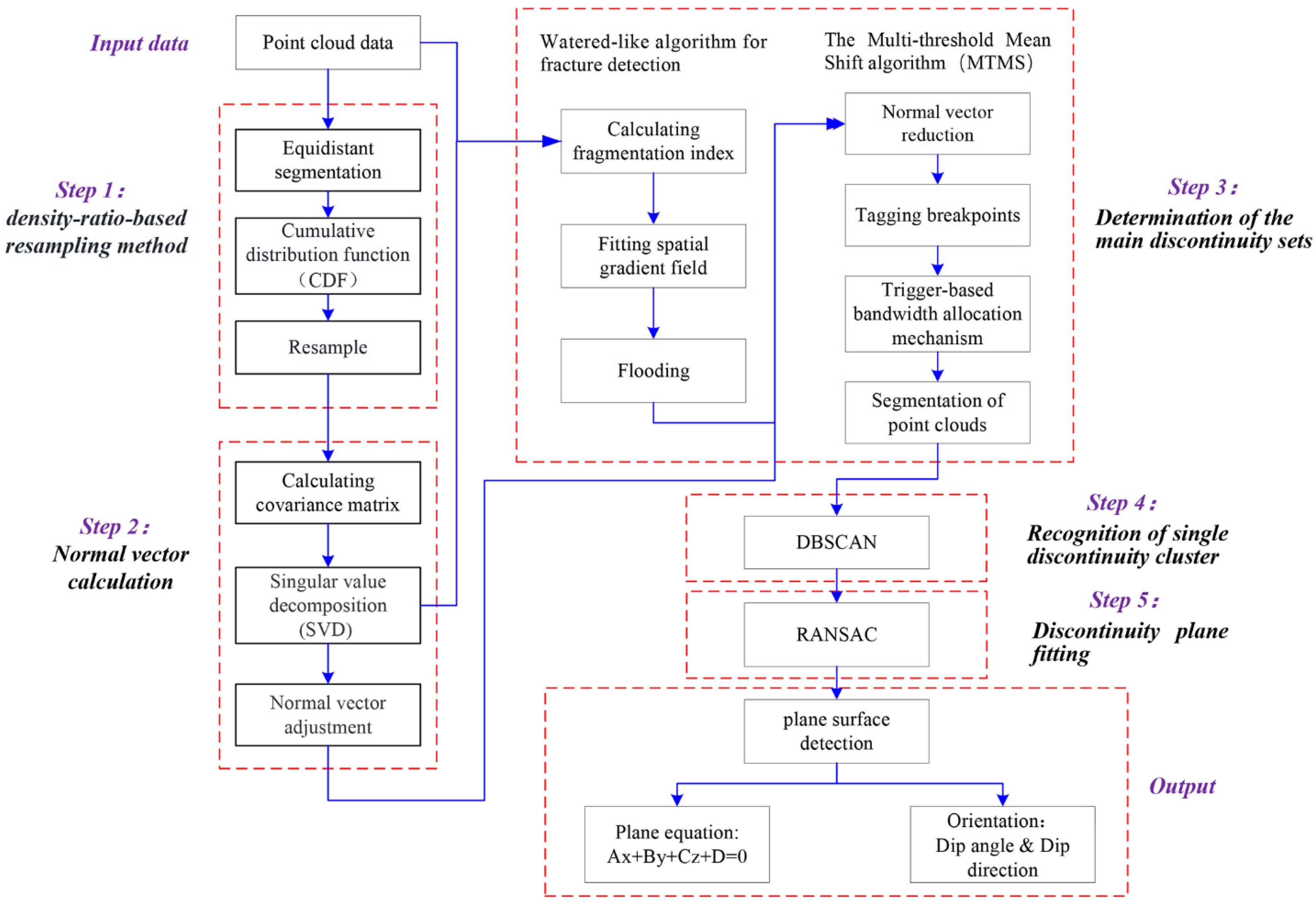
In this section, we introduce a workflow that integrates unsupervised clustering with RANSAC model fitting, utilizing a watershed-like algorithm to effectively address the issue of over-segmentation in rock discontinuities. The methodology is structured into five main steps:

Step 1: Adaptive resampling of the point cloud data based on density ratio, transforming the dataset through adaptive scaling according to density ratio. This task is detailed in Section 2.2.

Step 2: Estimating normal vector using Principal Component Analysis (PCA) and orienting them in the positive direction. This task is outlined in Section 2.3.

Step 3: Determination of the main discontinuity sets, which includes: (1) Applying a watershed-like algorithm to identify the non-planar areas of the discontinuities. This part is described in Section 2.4.2. (2) Segmenting the dominant discontinuity sets using the Multi-threshold Mean Shift (MTMS) algorithm. This part is covered in Section 2.4.3.

Step 4: Recognizing individual discontinuity clusters within each set using the DBSCAN algorithm. This task is explained in Section 2.5.

Step 5: Fitting a plane to each cluster from Step 4 using the RANSAC algorithm and calculating the orientation of each discontinuity. This task is described in Section 2.6.

A summary of this procedure is illustrated in Figure 1.

2.1. Description of the Experimental Datasets

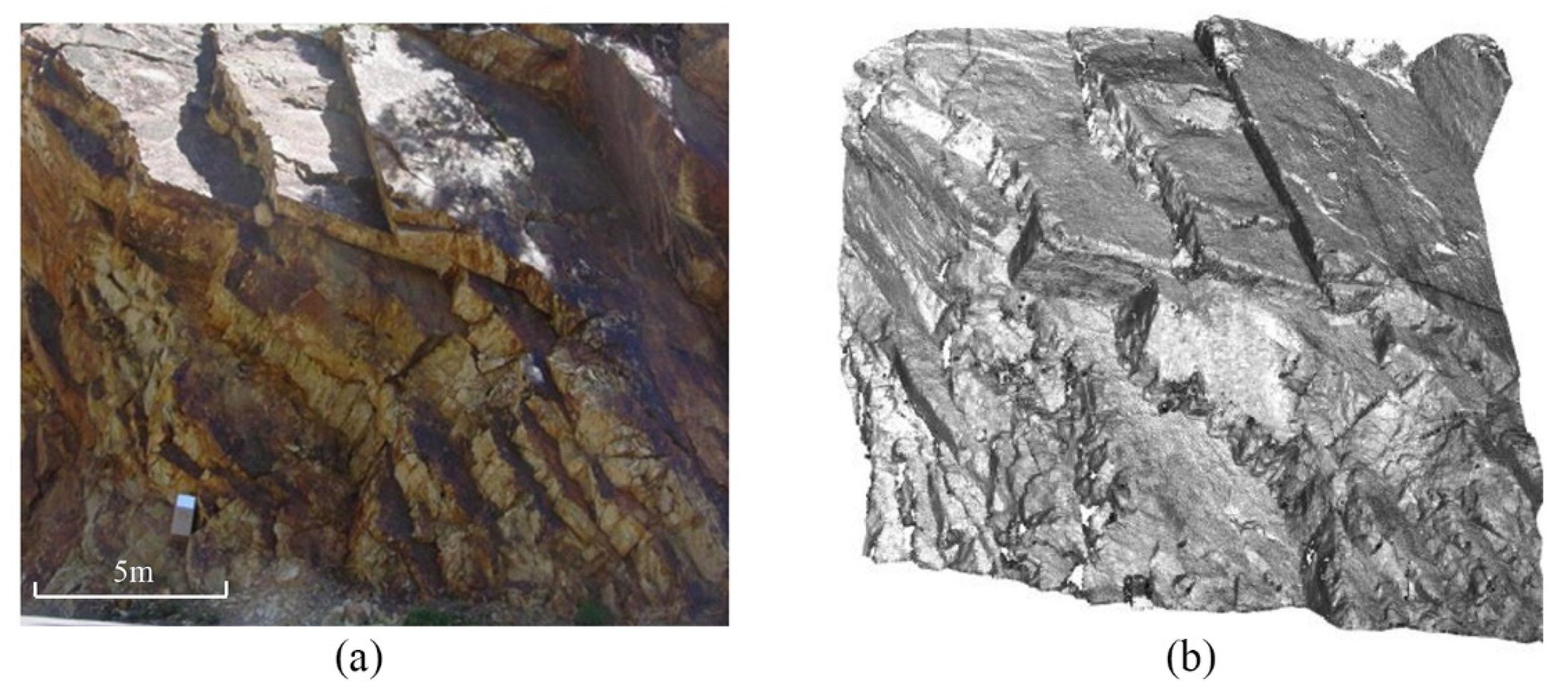
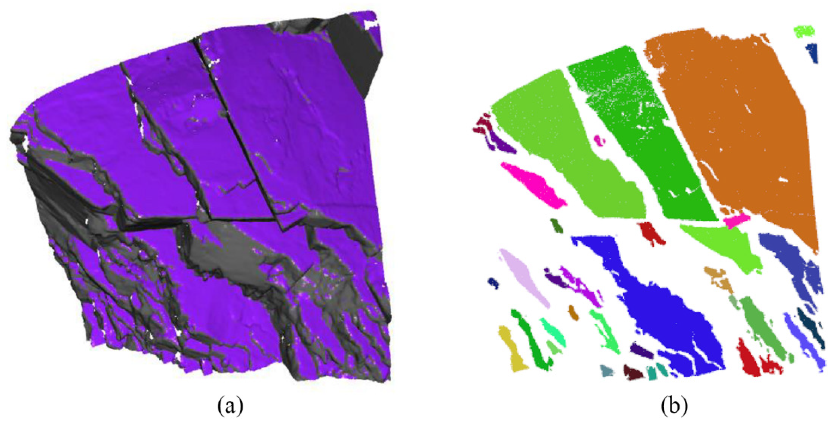
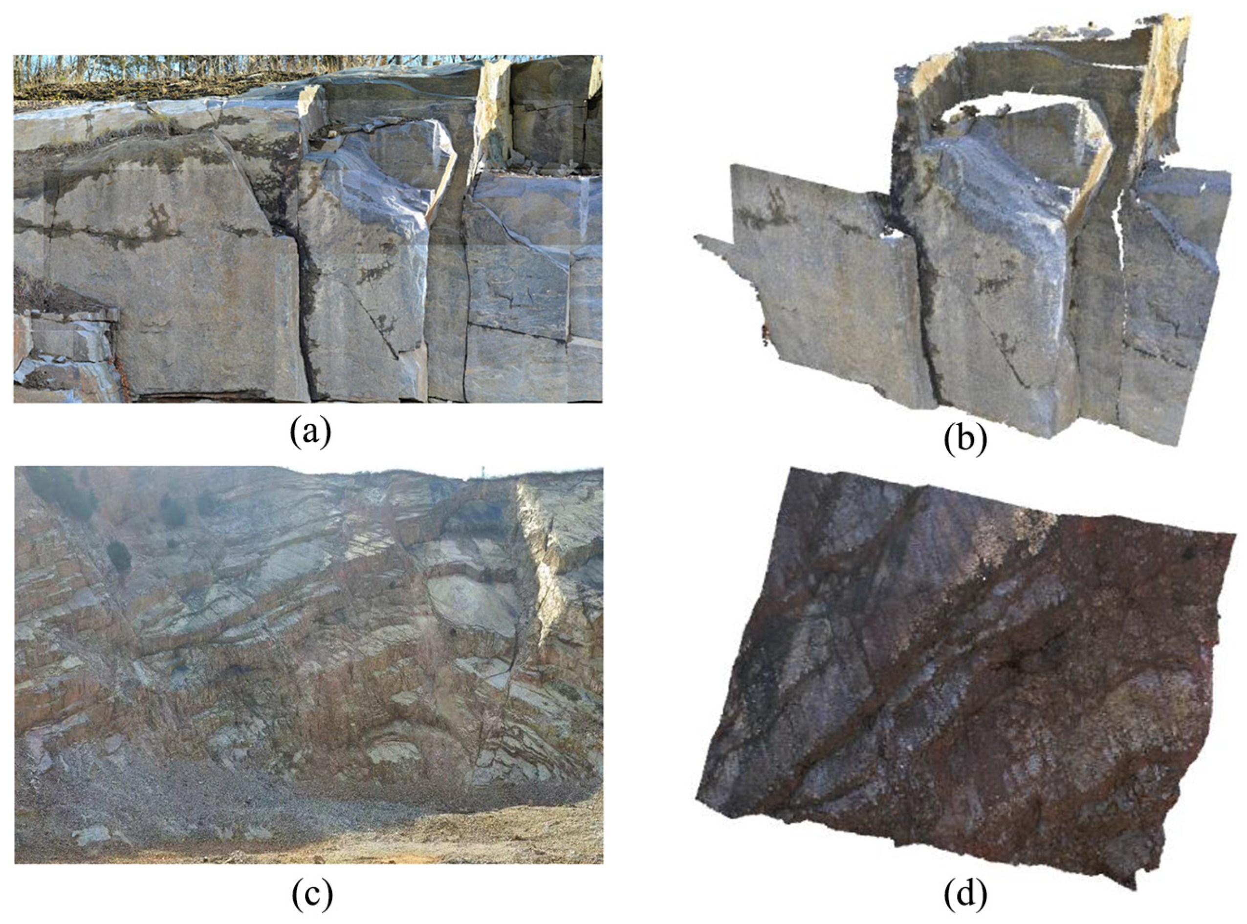
The experimental dataset used in this study originates from a quarzitic rock mass at a road cut slope in Ouray, CO, USA (Figure 2a). It was acquired from the Rock bench repository [43] using an Optech Ilris 3D Laser Scanner. It consists of 1,515,722 points with an average point spacing of approximately 2 cm. Figure 2b shows its corresponding trimmed point cloud, which contains 1,024,521 points. This dataset is a popular resource in the fields of geotechnical and geological engineering for estimating the orientations of structural surfaces. In previous studies, two sets of ground truth orientations have been documented. Numerous researchers have created both semi-automatic and fully automatic methodologies to determine the orientations of structural surfaces within this point cloud.

2.2. Density-Ratio-Based Resampling Method

Point cloud data obtained from laser scanning often suffer from issues like uneven data density distribution due to factors such as vegetation cover, occlusion, and noise. Density-based clustering algorithms, such as DBSCAN, are highly sensitive to variations in point cloud density and struggle to detect all clusters in datasets with significantly varying densities. Therefore, in our method, we draw inspiration from an image processing technique known as histogram equalization. This technique applies nonlinear stretching to an image, redistributing the grayscale values so that the grayscale levels within a certain range become approximately equal. The most common method for equalization is the Cumulative Distribution Function (CDF).

Based on this principle, we substitute the grayscale values with the local point density of the point cloud and use a density estimation algorithm as the density estimator to estimate the local density of each sampled point. We then resample the data according to the CDF estimated over a neighborhood ($\eta$). The effect of this process is to achieve a roughly uniform spatial distribution of the data [44]. This step enhances the accuracy of the DBSCAN algorithm in recognizing single discontinuity clusters, as described in Section 2.5. The key symbols and notations utilized in this study are provided in

Table 1. Symbols and notations.

$x$	The current sampling point
$D$, $S$	a d-dimensional dataset with n instances
$\epsilon$, $\eta$	radius of neighborhood
$\psi$	number of intervals for histogram
$pdf(·)$	probability density function
$\widehat{pd{f}_{\eta }}(·)$	the average density of the sampling point within the neighborhood $\eta$
$\widehat{pd{f}_{\epsilon }}(·)$	the average density of the sampling point within the neighborhood $\epsilon$
$\widehat{cd{f}_{\eta }}(·)$	The CDF of the sampling point within the neighborhood $\eta$
${\widehat{rpdf}}_{\epsilon ,\eta }(·)$	density-ratio estimation

.

The specific process is as follows.

(1)

The original dataset is $D$. When it is divided into $\psi$ equal intervals, the boundary positions are $\left\{x_1,x_2,\mathrm{\dots },x_{\psi +1}\right\}$;

(2)

At each boundary position $x_i$, calculate $\widehat{pd{f}_{\eta }}(x_i)={\displaystyle \frac{1}{2n\eta }}{\displaystyle {\sum }_j{\rm I}}\left(\Vert x_i-x_j\Vert \le \eta \right)$;

(3)

Calculate the resampled dataset: ${\forall }_{x\in D,y\in S}y={\displaystyle {\sum }_{x_i\le x}\widehat{pd{f}_{\eta }}(x_i)}$.

The theoretical basis for steps (2) and (3) is as follows.

Let the CDF at the sampling point $x$ be $\widehat{cd{f}_{\eta }}(x)={\displaystyle {\int }_{-\infty }^x\widehat{pd{f}_{\eta }}(x\prime )}dx\prime$. We define the cumulative distribution function. We resample the dataset $D$ into $S$ using the follow mapping function:

$${\forall }_{x\in D,y\in S} y=\widehat{cd{f}_{\eta }}(x)$$

(1)

This is a probability integral transform, where ${\forall }_{x\in D,y\in S} \widehat{pd{f}_{\eta }}(y)=\widehat{pd{f}_{\eta }}(\widehat{cd{f}_{\eta }}(x))=1/n$, representing a uniform distribution function.

Specifically, let $\widehat{pd{f}_{\epsilon }}(y)$ be the average density of $y=\widehat{cd{f}_{\eta }}(x)$ within a neighborhood of size $\epsilon <\eta$, then its density in the complete space is expressed as:

$$\begin{array}{ll}\widehat{pd{f}_{\epsilon }}(y)& ={\displaystyle \frac{1}{2n\epsilon }}{\displaystyle \sum _j{\rm I}\left(\Vert y-y_j\Vert \le \epsilon \right)}\\ & ={\displaystyle \frac{1}{2n\epsilon }}{\displaystyle \sum _j{\rm I}\left(\Vert \widehat{cd{f}_{\eta }}(x)-\widehat{cd{f}_{\eta }}(x_j)\Vert \le \epsilon \right)}\\ & \approx {\displaystyle \frac{1}{2n\epsilon }}{\displaystyle \sum _j{\rm I}\left(P_{X\sim \widehat{pd{f}_{\eta }}}\left(X\in \left[\min \left(x,x_j\right),\max \left(x,x_j\right)\right]\right)\le \epsilon \right)}\end{array}$$

(2)

When $n=\left|D\right|$ is large and varies slowly around $x$, this expression can be approximated as:

$$\begin{array}{ll}\widehat{pd{f}_{\epsilon }}(y)& ={\displaystyle \frac{1}{2n\epsilon }}{\displaystyle \sum _j{\rm I}\left(\widehat{pd{f}_{\epsilon }}(x)\ast \Vert x-x_j\Vert \le \epsilon \right)}\\ & \approx {\displaystyle \frac{1}{2n\epsilon }}{\displaystyle \frac{{\displaystyle \sum _j{\rm I}\left(\Vert x-x_j\Vert \le \epsilon \right)}}{\widehat{pd{f}_{\eta }}(x)}}\\ & ={\displaystyle \frac{\widehat{pd{f}_{\epsilon }}(x)}{\widehat{pd{f}_{\eta }}(x)}}\end{array}$$

(3)

Therefore, $\widehat{pd{f}_{\epsilon }}(y)\approx {\widehat{rpdf}}_{\epsilon ,\eta }(x)$, i.e., when resampling with a smaller $\epsilon$, the resampling result is scaled by different degrees according to the density ratio between the small neighborhood $\epsilon$ and the large neighborhood around the sampling point. In other words, when the sampling point $x$ is in a low-density region, the points in that area are less thinned out, while in a high-density region, the points are thinned out more significantly. This process is summarized in

Table 2. Resample the dataset $D$ into $S$ using the cumulative distribution function CDF.

Dataset	$\mathit{D}$ (Original Data)	$\mathit{S}$ (Resampled Data)
Instances	$x$	$y=\widehat{cd{f}_{\eta }}(x)$
Density estimator	$\widehat{pd{f}_{\epsilon }}(x)$	$\widehat{pd{f}_{\epsilon }}(y)={\widehat{rpdf}}_{\epsilon ,\eta }(x)$

.

2.3. Normal Vector Calculation

Accurate normal estimation in a point cloud is essential for effectively segmenting the desired plane features. Principal Component Analysis (PCA) is a statistical method that focuses on variation to uncover significant patterns in a dataset through an orthogonal transformation. PCA is widely used to identify local planar surfaces and linear points within a 3D point cloud. Using KD-tree nearest neighbor search, extract the neighborhood point sets (${\mathrm{D}}_1,{\mathrm{D}}_2,{\mathrm{D}}_3\cdots \cdots {\mathrm{D}}_{\mathrm{n}}$) for each sample point within the search radius (${\mathrm{R}}_1, {\mathrm{R}}_2, {\mathrm{R}}_3\cdots \cdots {\mathrm{R}}_{\mathrm{n}}$), respectively. Calculate the centroids of each neighborhood point set (${\mathrm{S}}_1, {\mathrm{S}}_2, {\mathrm{S}}_3\cdots \cdots {\mathrm{S}}_{\mathrm{n}}$). Construct the covariance matrices (${\mathrm{C}}_1, {\mathrm{C}}_2, {\mathrm{C}}_3\cdots \cdots {\mathrm{C}}_{\mathrm{n}}$) relative to the centroids, which reflect the correlation of each coordinate component in the point sets. The 3×3 covariance matrix for a sample point $p_i\left(x,y,z\right)$ can be written as:

$$C={\displaystyle \frac{1}{k}}{\displaystyle {\sum }_{i=1}^k{\left(p_i-\overline{p}\right)}^T\left(p_i-\overline{p}\right);}\overline{p}={\displaystyle \frac{1}{k}}{\displaystyle {\sum }_{i=1}^k{p}_i}$$

(4)

Utilize Singular Value Decomposition (SVD) on the covariance matrix of each point. The covariance matrix $C$ can be represented as:

$$C=\left[\begin{array}{ccc}{e}_1& e_2& e_3\end{array}\right]\left[\begin{array}{ccc}{\lambda }_1& 0& 0\\ 0& {\lambda }_2& 0\\ 0& 0& {\lambda }_3\end{array}\right]\left[\begin{array}{c}{e}_1^T\\ e_2^T\\ e_3^T\end{array}\right]$$

(5)

Among them, ${\lambda }_1,{\lambda }_2,{\lambda }_3$ are the eigenvalues of $C$, and $e_1$, $e_2$, $e_3$ are the corresponding eigenvectors. After normalizing the eigenvalues and sorting them by size, we have ${\lambda }_1\ge {\lambda }_2\ge {\lambda }_3>0$, where ${\lambda }_1$, ${\lambda }_2$ and ${\lambda }_3$ represent the fitting deviations in the directions of the corresponding eigenvectors of the local plane. The eigenvector corresponding to the smallest eigenvalue, ${\lambda }_3$, indicates the direction of the least variation in the point set distribution. This direction can be considered the normal direction of the local surface.

Since PCA can only provide a direction without distinguishing between “inward” and “outward”, an additional post-processing step is required to correct any normal vectors that are flipped by 180°. This study uses a method based on the continuity of normal directions to adjust and ensure the consistency of the normal vector orientations.

2.4. Determination of the Main Discontinuity Sets

Identifying group discontinuities is fundamental for pinpointing individual discontinuities, which is essential for accurately identifying rock discontinuities. This phase focuses on categorizing each point into a discontinuity group based on distribution patterns.

MS is a feature space analysis method that estimates the probability density distribution of feature data through Kernel Density Estimation (KDE). It clusters data points by moving them in the direction of increasing probability density until they converge at the local density maximum. The method can process point clouds of any shape without needing a predefined number of clusters. It requires only one parameter, the bandwidth size. The bandwidth determines the step size for each adjustment of the probability density function. For MS, tuning the bandwidth is the most critical hyperparameter.

2.4.1. The Impact of Bandwidth on MS

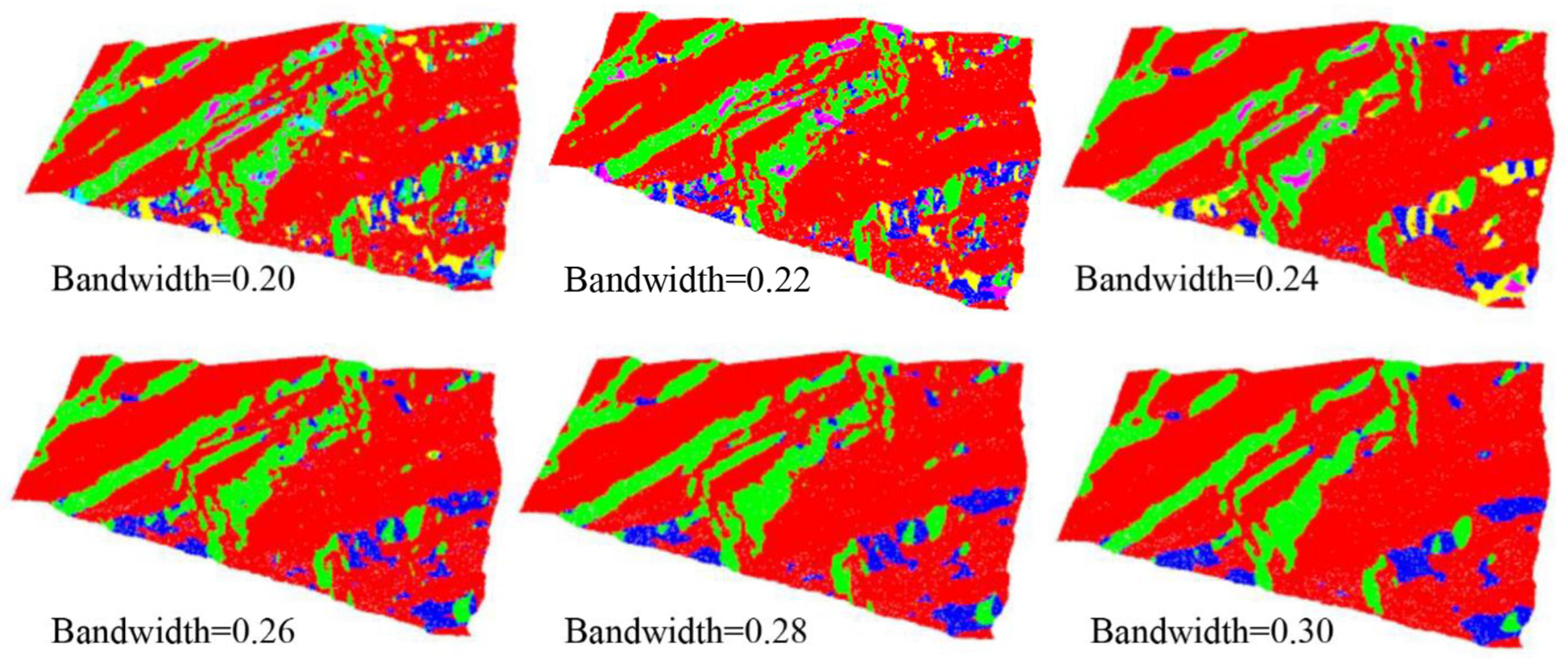
The bandwidth, as the sole input parameter for MS, has a crucial impact on the segmentation effect. Figure 3a illustrates the kernel density of a one-dimensional dataset. The dashed lines indicate the kernel function for each sample, while the solid line depicts the probability density of the dataset, which is the aggregate of the sample kernel functions. It can be observed that the probability density of this dataset has only one local maximum, so the current dataset is segmented into one cluster using MS with a bandwidth of 6. If we set the bandwidth to approach zero infinitely, the sample kernel functions will be as shown in Figure 3b, approximating impulse functions, and the probability density will be as shown in Figure 3c. The dataset will have five local maxima and be segmented into five clusters. Therefore, the bandwidth determines the probability density of the dataset. If the bandwidth is too large, MS may overly smooth the data, failing to capture local details and features, resulting in under-segmentation. Conversely, if the bandwidth is too small, it will include fewer points, leading to the amplification of some local details and features, causing over-segmentation.

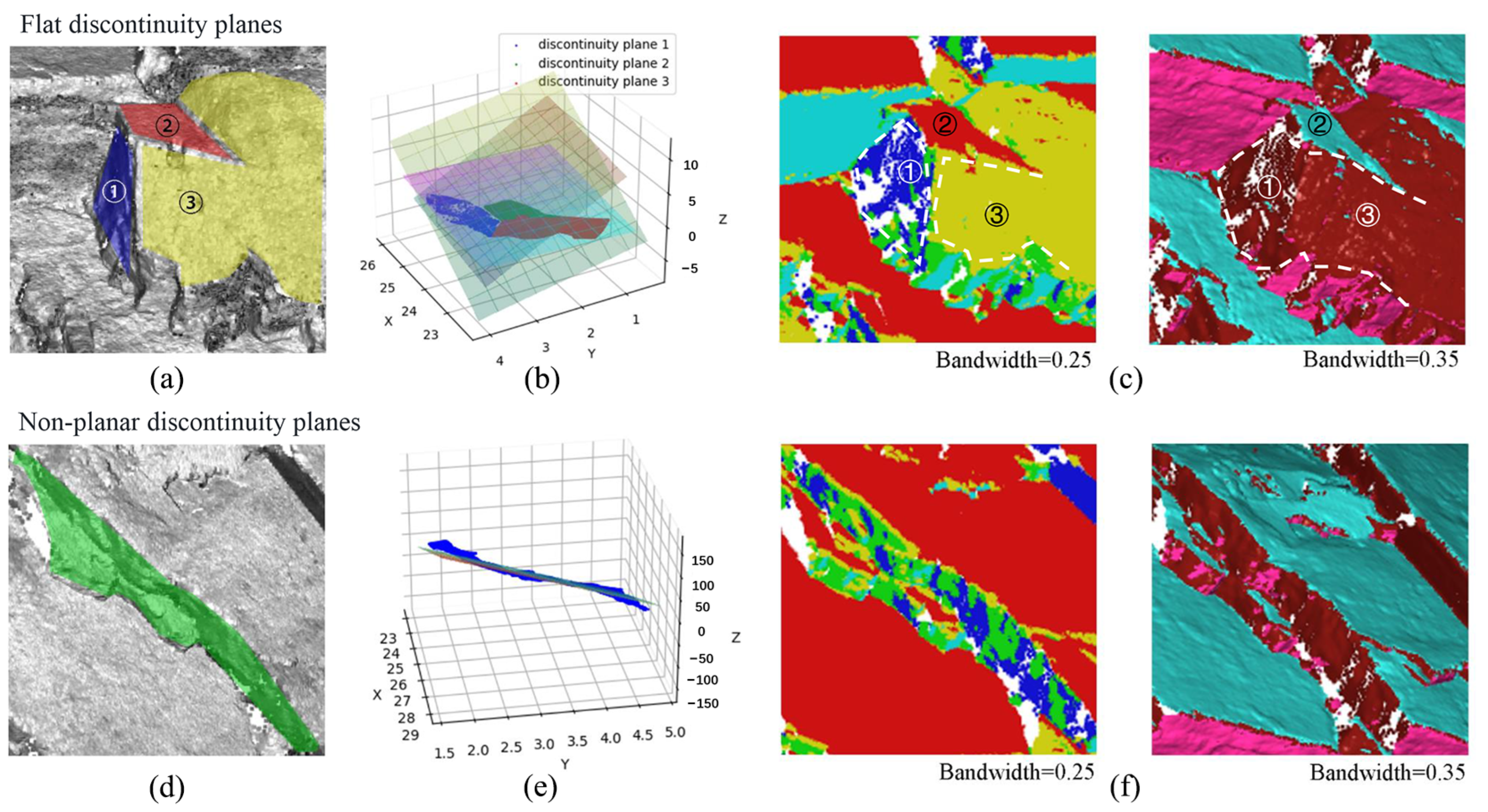
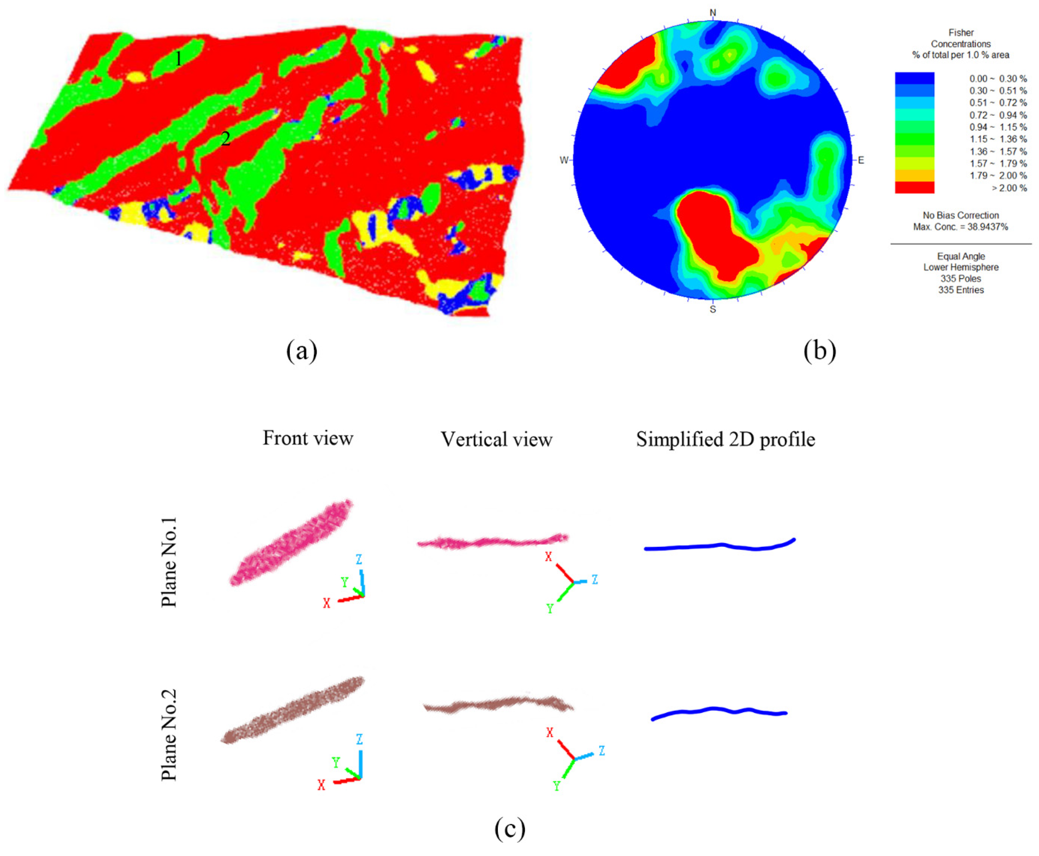
Figure 4 illustrates the effect of bandwidth on different types of discontinuities. Figure 4a shows a representative area of the experimental dataset with flat discontinuities. The spatial orientation of plane 1, plane 2, and plane 3 is illustrated in Figure 4b, where each plane belongs to a different set of discontinuities. By comparing segmentation effects with different bandwidths in this area, we find that the segmentation effect in Figure 4c with a bandwidth of 0.25 is ideal because it effectively segments the area into three discontinuities while preserving edge details. For the non-planar discontinuities targeted in this study (Figure 4d), Figure 4e simulates their planes in 3D space. It is clear that the non-planar discontinuities fit well with the plane model, suggesting that most points on the non-planar discontinuities should theoretically be classified into the same discontinuities set. Figure 4f shows the segmentation effect of using different bandwidths for MS in this area. When the bandwidth is 0.25, the points are over-segmented. To avoid over-segmentation, the bandwidth is increased, and the result obtained with a bandwidth of 0.35 is considered the most suitable representation because most points in this area are assigned to the same discontinuities set. However, for flat discontinuities, when the bandwidth is 0.35 (see Figure 4c), plane1 and plane3 are assigned to the same discontinuities set, resulting in under-segmentation.

Based on the comprehensive analysis above, it is evident that the optimal bandwidth for non-planar discontinuities and flat discontinuities differs. However, most existing MS methods use a global fixed bandwidth [22,26]. To ensure accuracy, this often leads to over-segmentation in areas with non-planar discontinuities. On the other hand, expanding the threshold range can reduce accuracy when segmenting flat discontinuities. This makes it difficult to balance both types of discontinuities within the same dataset, leading to over-segmentation or under-segmentation. Therefore, it is necessary to identify non-planar areas and set different bandwidths for points located in these areas and those in flat discontinuities. To tackle this issue, we propose a new method for detecting individual discontinuities, which primarily includes: (1) applying a watershed-like algorithm to identify non-planar areas of discontinuity. (2) using the Multi-threshold Mean Shift (MTMS) algorithm to segment the advantageous discontinuity sets. Detailed descriptions of these improvements are provided in the following subsections.

2.4.2. Watershed-like Algorithm for Identifying Non-Planar Areas

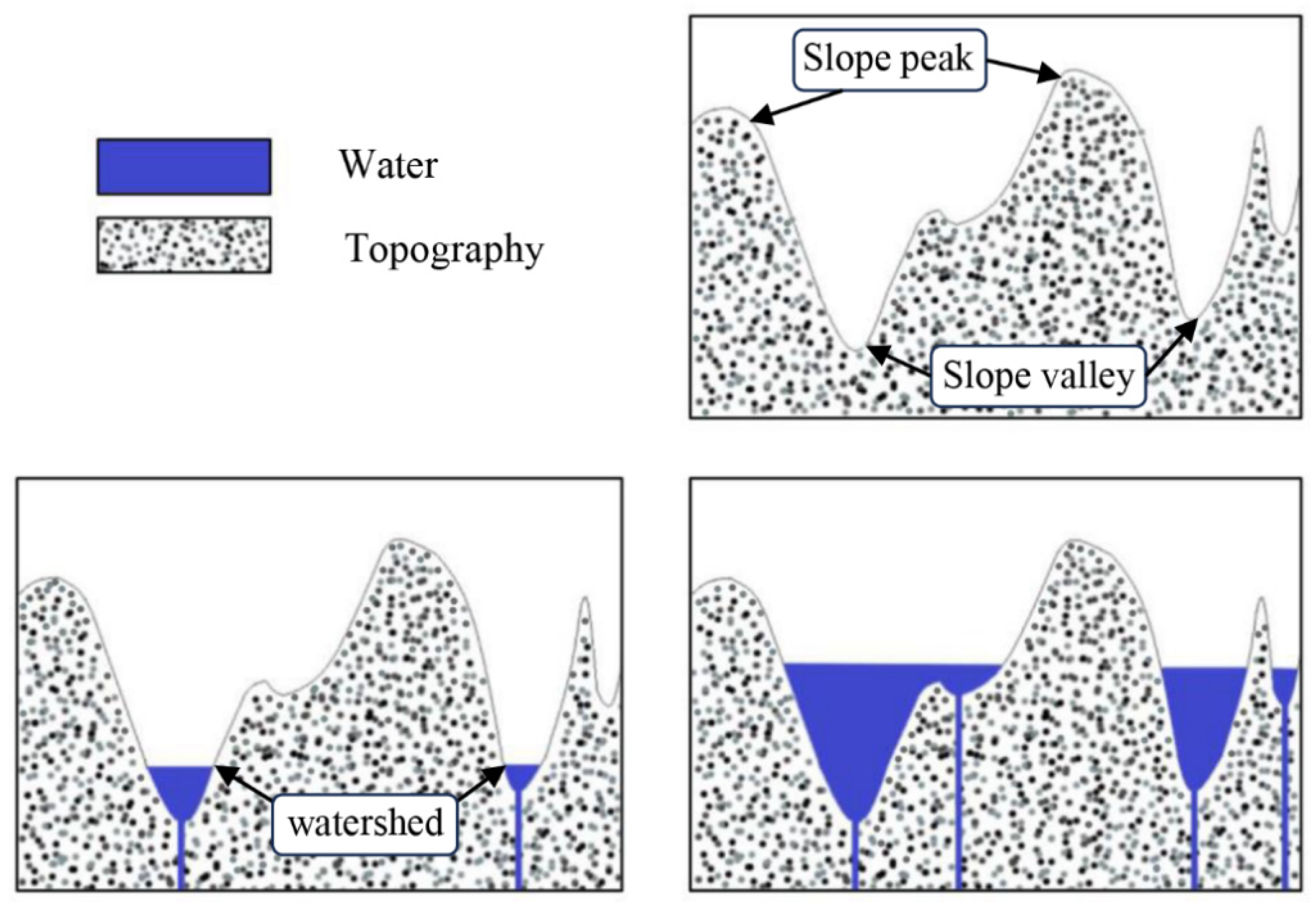
The Watershed algorithm is an image segmentation technique that separates and labels different regions within an image. It is based on the grayscale values or gradient information of the image, treating the depth image as a topographic map [45]. The algorithm assigns a gradient value to each pixel by calculating gradient operators, and simulating peaks and valleys (basins). As illustrated in Figure 5, assuming there are small holes on the surface of the minimal regions of the terrain, water seeps in through these holes and gradually floods the surrounding areas at a uniform rate, forming corresponding catchment basins. The boundary line of each catchment basin is known as the watershed line [46,47,48]. 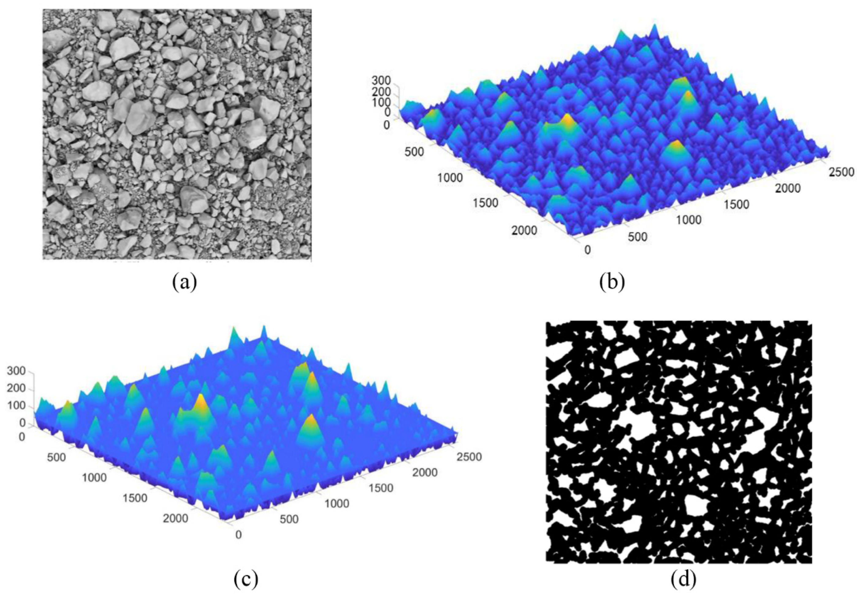Figure 6 demonstrates the Watershed algorithm’s segmentation process in an image [49]. Figure 6a shows a limestone-blasted grayscale image, treated as a gradient image, where the grayscale values at corresponding coordinates represent elevation. Figure 6b depicts the 3D simulation of the water catchment basin in this image, assuming a gray threshold of 50 as the watershed line. Figure 6c shows the 3D simulation post-flooding, and Figure 6d presents the segmented 2D cross-section.

Current researchers are exploring the application of watershed-like concepts or modified algorithms to point cloud data, as the density or other attributes of point clouds may, to some extent, resemble “height” or “intensity”. By simulating this analogy, “terrain” in 3D space can be defined. Based on this idea, this paper proposes a watershed-like algorithm that uses non-planar indicators as gradient operators to restrict the flooding process of the watershed algorithm, thereby better identifying non-planar regions of discontinuities.

Calculate the Non-Planar Indicator

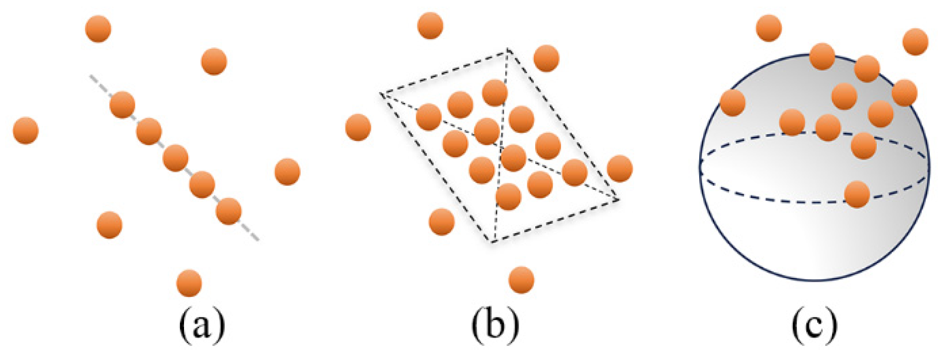
In Section 2.3, we used PCA to compute the local covariance matrix eigenvalues ${\lambda }_1$, ${\lambda }_2$, ${\lambda }_3$ as shown in Equation (2). According to the theory of Demantké et al., as shown in Figure 7, the eigenvalues can represent the dimensional properties of the local neighborhood within the point cloud [50]. When ${\lambda }_1\gg {\lambda }_2\cong {\lambda }_3$, the local neighborhood of the point cloud tends to be rod-shaped; when ${\lambda }_1\cong {\lambda }_2\gg {\lambda }_3$, the local neighborhood of the point cloud tends to be planar; when ${\lambda }_1\cong {\lambda }_2\cong {\lambda }_3$, the local neighborhood of the point cloud tends to be a three-dimensional surface.

Therefore, we construct a local neighborhood dimension feature model based on these dimensional characteristics [51]:

$$L_{\lambda }={\displaystyle \frac{\sqrt{{\lambda }_1}-\sqrt{{\lambda }_2}}{\sqrt{{\lambda }_1}}},P_{\lambda }={\displaystyle \frac{\sqrt{{\lambda }_2}-\sqrt{{\lambda }_3}}{\sqrt{{\lambda }_1}}},S_{\lambda }={\displaystyle \frac{\sqrt{{\lambda }_3}}{\sqrt{{\lambda }_1}}}$$

(6)

In the study by Demantké et al. [50], the dimensional features $L_{\lambda }$, $P_{\lambda }$ and $S_{\lambda }$ can, respectively, represent the probability that the local neighborhood of the point is a one-dimensional line, a two-dimensional plane, or a three-dimensional surface [50]. The planar dimension feature $P_{\lambda }$ indicates how well the local neighborhood of the point cloud aligns with a plane. The closer the point is to a planar structure, the larger its corresponding dimension feature $P_{\lambda }$. Therefore, this paper defines an indicator to describe the curvature of the local neighborhood:

$$\omega ={(1-P_{\lambda })}^2$$

(7)

From Equation (7), it can be observed that the smaller the value of $\omega$, the closer the local neighborhood shape is to a plane. When the local neighborhood is a curved surface, the value corresponding to $\omega$ is a fixed value related to the curvature of the surface.

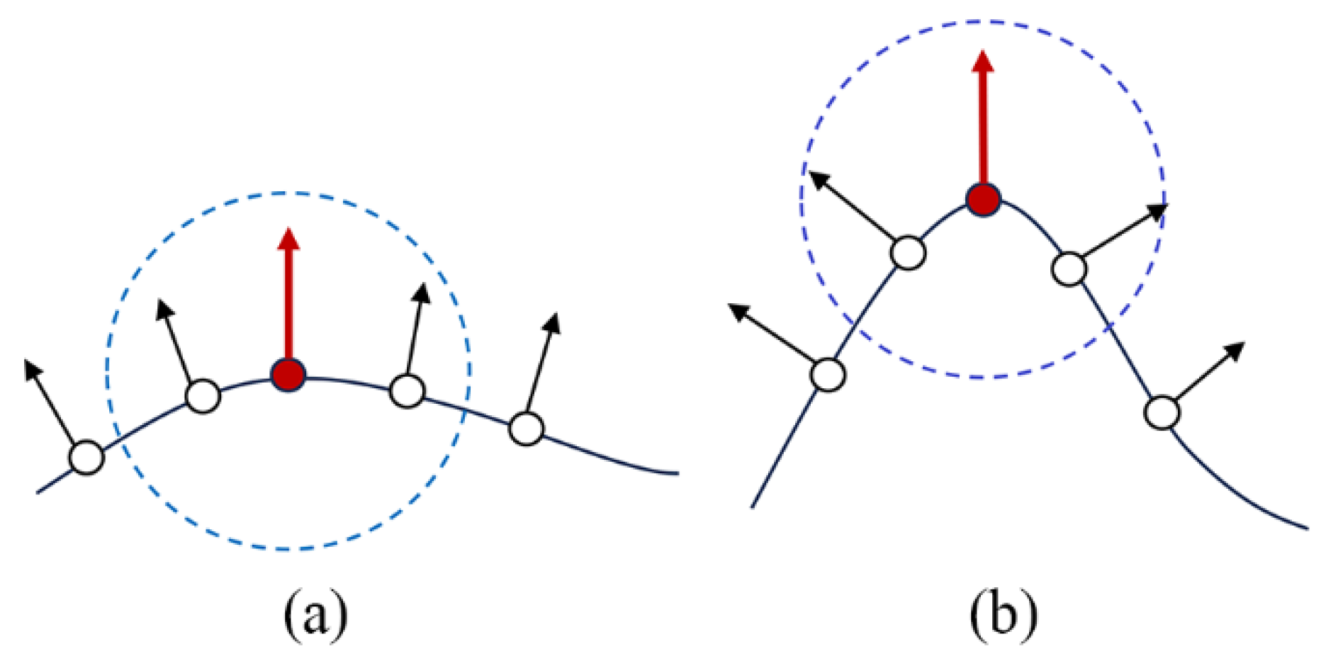
To distinguish between non-planar and flat areas, as shown in Figure 8, surfaces with different degrees of curvature have varying normal direction deviations within the same neighborhood range. The more curved the surface, the greater the deviation in the normal direction. Therefore, we use the angle between the normal vectors of the sampling point and its neighboring points as a reference factor.

To simplify the complex curvature calculation process, we establish a local neighborhood $V_r$, centered on the sampling point. The size of $V_r$ is customized according to the scale of the rock mass. Given that the number of neighborhood points within $V_r$ is $k$, the curvature at the sampling point is defined as follows:

$$C={\displaystyle \frac{1}{k}}{\displaystyle {\sum }_{i=1}^k{\lambda }_i}$$

(8)

where ${\lambda }_i$ represents the deviation between the sampling point and the normal vectors of the neighboring points within the local neighborhood. It can be observed that as ${\lambda }_i$ increases, indicating a greater degree of bending in the local structure, the curvature value correspondingly increases.

Combining the two-dimensional feature $\omega$, this paper defines a non-planar indicator:

$$K=C\ast \omega$$

(9)

where $C$ is an indicator that measures the degree of bending within the local neighborhood, and $\omega$ describes the curvature of the local neighborhood. The shape characteristics of the point cloud’s local neighborhood are determined based on the non-planar indicator $K$. When the local neighborhood is close to being planar, the non-planar indicator approaches 0. As $K$ increases, it indicates a greater degree of bending in the local neighborhood of the point cloud.

Fitting Spatial Gradient Fields

Due to the similarity in curvature among closely spaced points, we sample the point cloud data to reduce computational load and improve efficiency. A voxelized grid method is used to create a voxel grid, which consists of 3D boxes in space, to encompass the input point cloud. The voxel size is determined by the user based on specific requirements. To sample feature points, select point $p_{centroid}$ located at the centroid of each voxel, and calculate the non-planar indicator $K$ for each feature point in the experimental dataset. 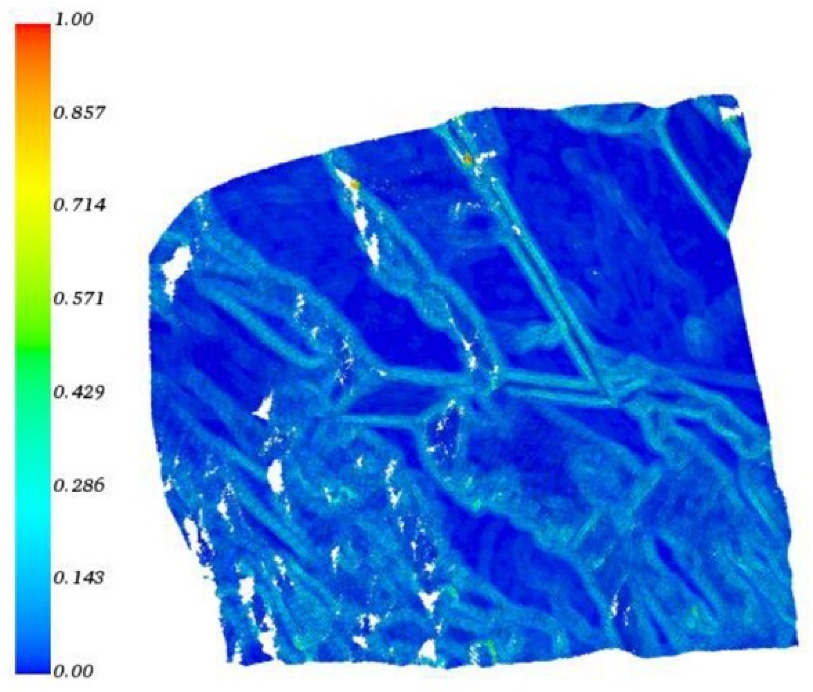Figure 9 is an HSV simulation diagram of the experimental dataset colored according to the non-planar indicator $K$. It can be observed that the values of $K$ in this dataset primarily range $0\sim 0.2$, The smaller the $K$ value, the flatter the region where the point is located; the larger the $K$ value, the more curved the point’s location is. We use the ascending $K$ values to simulate the elevation from valleys (basins) to peaks in the high-dimensional features, with the peaks representing the non-planar areas we aim to identify.

The watershed algorithm typically processes gradient data [52]. In this study, the Sobel operator is used to calculate the gradient data of the voxels $V$. Assuming $V_{LT}$, $V_{RT}$, $V_{LU}$, $V_{RU}$, $V_{FT}$, $V_{BT}$, $V_{FU}$, $V_{BU}$, $V_T$, $V_U$, $V_L$, $V_R$, $V_F$, $V_B$ represent the points in the 14-neighborhood of voxel $V$ in the directions: top-left, top-right, bottom-left, bottom-right, front-top, back-top, front-bottom, back-bottom, top, bottom, left, right, front, and back, respectively. The gradient values of voxel V in the x, y and z directions, denoted as $d_x(V)$, $d_y(V)$ and $d_z(V)$, are given by:

$$\{\begin{array}{l}{d}_x(V)=\left[K(p_{RT})+2K(p_R)+K(p_{RU})\right]-\left[K(p_{LT})+2K(p_L)+K(p_{LU})\right]\\ d_y(V)=\left[K(p_{LT})+2K(p_T)+K(p_{RT})\right]-\left[K(p_{LU})+2K(p_U)+K(p_{RU})\right]\\ d_z(V)=\left[K(p_{FT})+2K(p_F)+K(p_{FU})\right]-\left[K(p_{BT})+2K(p_B)+K(p_{BU})\right]\end{array}$$

(10)

The gradient magnitude $d(\mathrm{V})$ is:

$$d(V)=\sqrt{{\left[d_x(V)\right]}^2+{\left[d_y(V)\right]}^2+{\left[d_z(V)\right]}^2}$$

(11)

For each point $p_i$, in the point cloud data, assuming the index of its voxel is $V_{p_i}$, we approximate the gradient value $d(p_i)$ of the point $p_i$ as being equal to the gradient value of the voxel it resides in, that is

$$d(p_i)=d(V_p)$$

(12)

Since point cloud data exist in 3D space, it is not feasible to simulate ridges and valleys on the same horizontal plane as one would with images. To facilitate the simulation of the watershed inundation process, we use the normal direction of each point as the vertical direction of the peaks. Through this approach, we define the “terrain” in the multidimensional space, allowing for more convenient simulation and analysis.

To determine the frequency distribution of each gradient level, we need to utilize a sorting algorithm to arrange the experimental dataset by gradient magnitude. Each point is then assigned to an ordered queue corresponding to its gradient level. Assume the number of gradient levels is $N$:

$$N=\mathrm{INT}\left({\displaystyle \frac{d_{\max }-d_{\min }}{d_{gap}}}\right)$$

(13)

where $d_{\max }$ is the maximum gradient value, $d_{\min }$ is the minimum gradient value, $d_{gap}$ is the interval of the gradient levels, and INT denotes the rounding operation.

The gradient level $K_p$ at point $p_i$ is shown as

$$K_p=\mathrm{INT}\left[{\displaystyle \frac{d(p)-d_{\min }}{d_{gap}}}\right]+1$$

(14)

From Equation (13), it can be seen that the gradient level interval $d_{gap}$ determines the number of gradient levels N, which in turn determines the number of points submerged during each step of the flooding process. According to Equation (14), the gradient level for each point can be calculated. The flooding process submerges points sequentially according to their gradient levels.

Flooding

First, let us clarify some basic concepts in this method:

Minimum Region: The minimum region $M$ is an independent connected area where the gradient values within the region are lower than the gradient values of the surrounding neighboring points.

Water Catchment Basin: The water catchment basin $B\left(M\right)$ is an area composed of a collection of points within the experimental dataset that form the minimum region $M$. Within the water catchment basin, water flow from any location will slide down along a certain path to reach the minimum region $M$.

Geodesic Distance: Assuming $S$ is a connected region, the geodesic distance $D_S(j,k)$ is along the geodesic path from $j$ to $k$ within $S$.

Geodesic Influence Region: Let set $S$ contain set $W$, where $W$ consists of multiple connected regions $W_1,W_2,\cdots ,W_k$. Within set $S$, if there exists a point set $Q$ whose geodesic distance to connected region $W_i$ is shorter than its distance to any other connected region within set $W$, then $Q$ is considered the geodesic influence region $Z_S(W_i)$ of connected region $W_i$.

The flooding process is essentially a recursive process. Suppose the experimental dataset is $E$, and $T_f(p)$ is the threshold set for point $p$ at level $f$,

$$T_f(p)=\left\{p\in E,K_p\le f\right\}$$

(15)

The flooding process starts from the threshold set $T_1(p)$, which is the set of points with the smallest gradients. Let the collection of first-level basins be:

$$U_1=T_1(p)$$

(16)

Let n be the gradient level, and the recursive process of the $f$-th level basin $U_f$ is

$$\forall f\in \left[1,n-1\right],U_{f+1}\cup Z_{T_{f+1}(p)}(U_f)$$

(17)

The set of catchment basins with $w$ as the watershed line is

$$U_w={\displaystyle {\sum }_1^{w-1}\left\{U_{i+1}\cup Z_{T_{i+1}(p)}(U_i)\right\}}$$

(18)

For the experimental dataset $E$, the set of non-planar areas $H_w$ (slope peaks) is

$$H_w=E-U_w$$

(19)

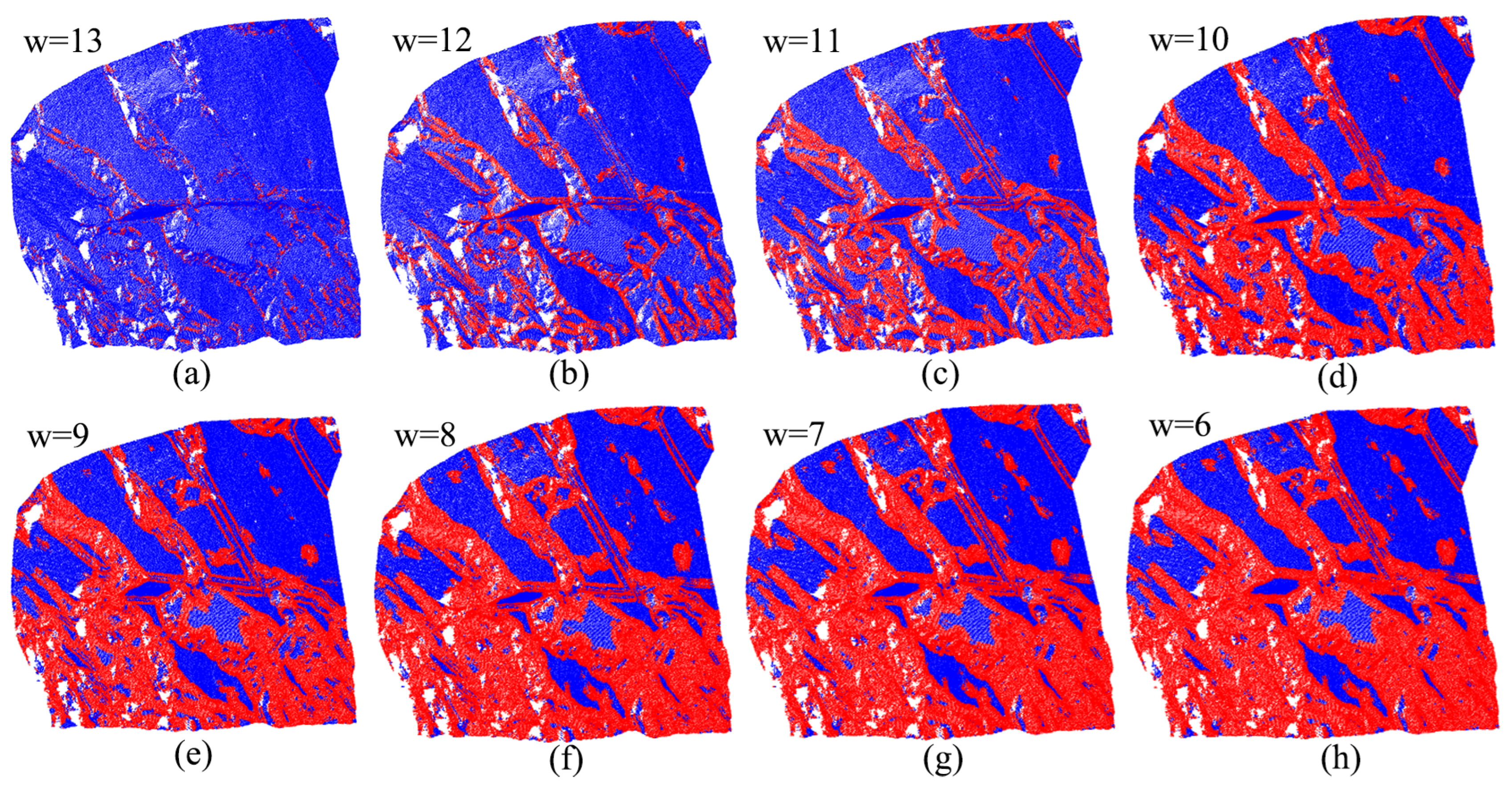
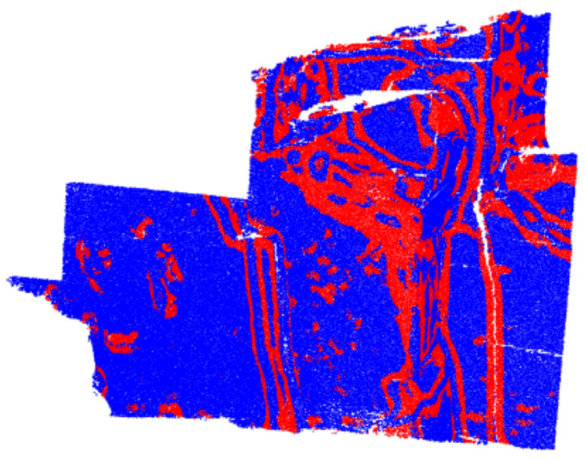
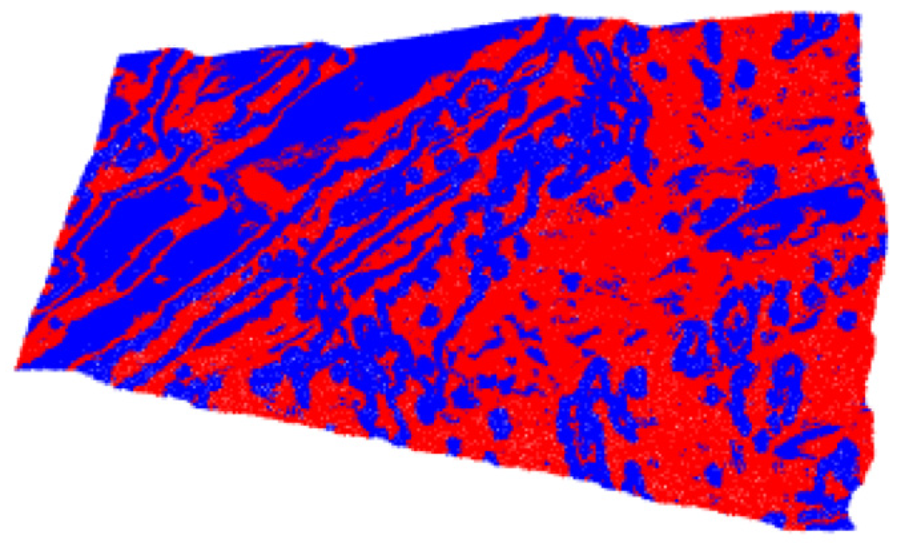
According to Equation (18), the watershed line $w$ determines the range of slope peaks and valleys. For the experimental dataset, we set the number of gradient levels to $N=15$, Figure 10 shows a comparison of the flooding results for different watershed lines, where the red area represents the non-planar area (slope peaks). It can be observed in Figure 10a–f that as the value of $w$ decreases, the range of the identified non-planar area gradually increases. However, in Figure 10g,h, even though $w$ continues to decrease, the range of the identified non-planar area remains almost unchanged. The study found that there exists a critical value for the watershed line, which distinguishes between planar areas and non-planar areas—essentially, the cliff edge of the peak. Due to the significant gradient difference between planar areas and non-planar areas, the identification results remain nearly constant when $w$ continues to decrease. In the experimental dataset, $w=8$ represents the critical value of the watershed line, where the division at the peak of the slope accurately reflects the location of non-planar area. Therefore, we use $w=8$ as the watershed line for the experimental dataset.

2.4.3. The Multi-Threshold Mean Shift (MTMS) Algorithm

Currently, most discontinuity recognition methods based on MS employ a fixed bandwidth. However, using a single global bandwidth for rock slopes with numerous non-planar areas is not optimal, as a single global value may result in over-segmentation or under-segmentation. Section 2.4.1 provides a detailed explanation of the impact of bandwidth on segmentation performance. MTMS is an improvement over the traditional MS method. This approach assigns different bandwidths to points in planar and non-planar areas during the shifting process. By doing so, it controls the step size of the probability density function adjustment for points in different regions. This method achieves a better balance between local and global features. The specific process is shown in Figure 11.

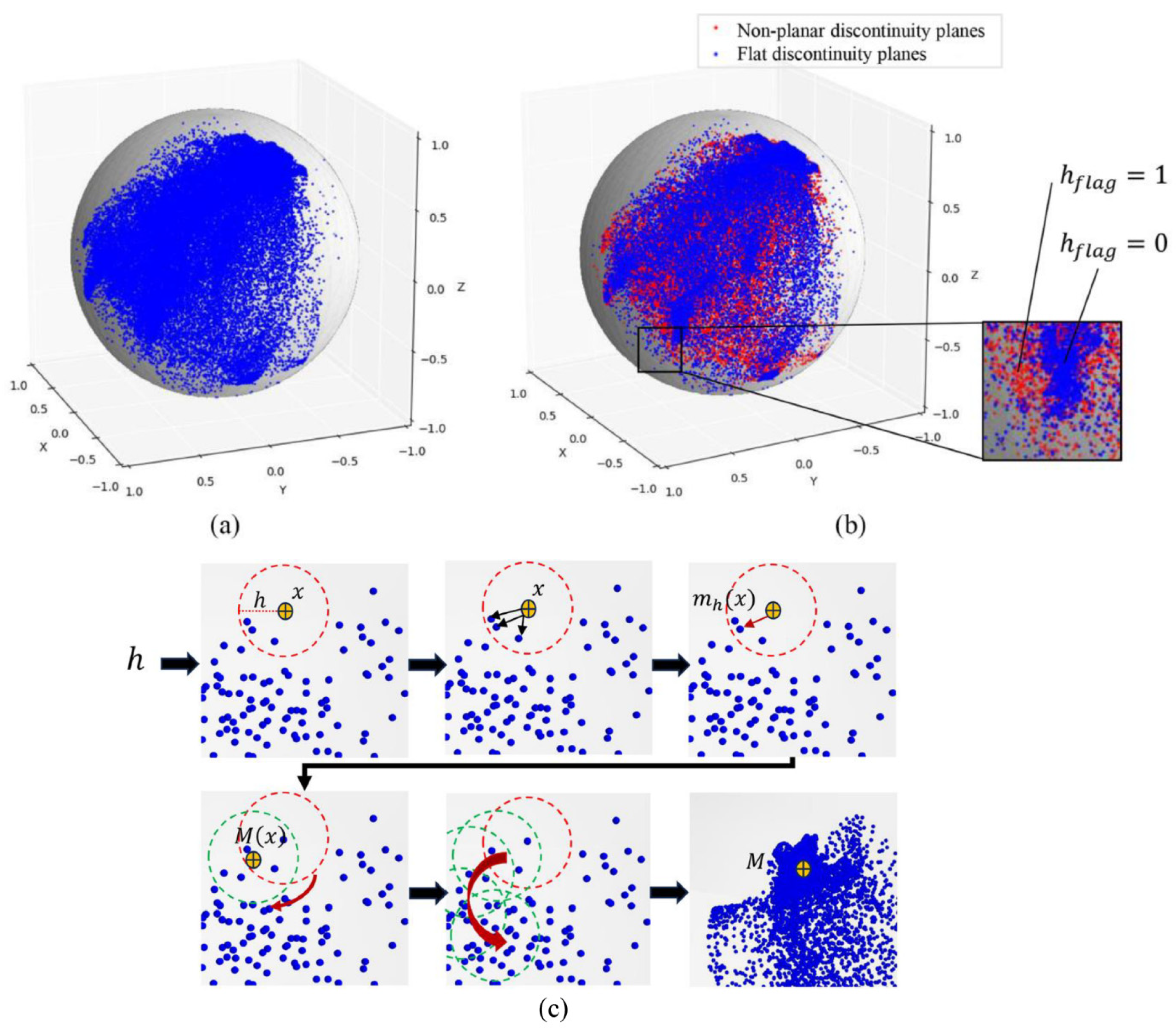
Map the estimated normal vectors from Section 2.3 to the feature space, extending from a 2D Gaussian surface to a 3D Gaussian sphere (Figure 11a), as the input for MTMS. Define a flag value to mark whether a point is in a non-planar area. Search for the points located in the non-planar area defined in Section 2.4.2 in spherical coordinates, setting their flag to 1, while setting the flag to 0 for the remaining points. The resulting binary map is shown in Figure 11b.

Based on the flag, construct a trigger-based bandwidth allocation mechanism as detailed in Figure 11c. Randomly select a point from all unprocessed points as the center point, check its flag label, and if flag = 1, set its bandwidth to $h_{flag=1}$; if flag = 0, set its bandwidth to $h_{flag=0}$. The kernel function of MS assigns certain weights to points around each point. In the feature space, it weights the points within a specified bandwidth region around the current center point to estimate the local density. The density calculation formula is

$$f(x)={\displaystyle \frac{1}{n{h}^d}}{\displaystyle \sum _{i=1}^{n}K\left(\frac{x-x_i}{h}\right)},$$

(20)

where $K(x)$ is the kernel function weight formula, $n$ is the number of features, $h$ is the bandwidth of the current search point, $d$ is a normalization constant that ensures $K(x)$ = 1.

Calculate the gradient direction of the dataset density, which is the direction of the fastest increase in local density, to obtain the drift vector. The gradient of the density function is:

$$\nabla f(x)={\displaystyle \frac{2C_{k,d}}{n{h}^{d+2}}}{\displaystyle \sum _{i=1}^n(x_i-x)}\left[{\displaystyle \frac{{\displaystyle \sum _{i=1}^n{x}_{i}g\left({\Vert \frac{x-x_i}{h}\Vert }^2\right)}}{{\displaystyle \sum _{i=1}^{n}g\left({\Vert \frac{x-x_i}{h}\Vert }^2\right)}}}-x\right],$$

(21)

where ${\displaystyle \frac{2C_{k,d}}{n{h}^{d+2}}}{\displaystyle \sum _{i=1}^n(x_i-x)}$ is a real number, so the drift vector is

$$m_h(x)={\displaystyle \frac{{\displaystyle \sum _{i=1}^n{x}_{i}g\left({\Vert \frac{x-x_i}{h}\Vert }^2\right)}}{{\displaystyle \sum _{i=1}^{n}g\left({\Vert \frac{x-x_i}{h}\Vert }^2\right)}}}-x$$

(22)

Translate the sample point x iteratively according to the drift vector. The center point for the next iteration is

$$M(x)=x+m_h(x_i)$$

(23)

Repeat the iteration several times until $m_h(x_i)=0$, so that the samples converge to the local density peak, resulting in multiple sets of dominant points with similar principal directions.

2.5. Recognition of Single Discontinuity Cluster

To distinguish each individual planar surface among many planes with similar orientations in the primary cluster, secondary clustering is required. Within each discontinuity set, each single discontinuity creates a dense region in space, resulting in a density difference between the discontinuities. This characteristic makes them ideal for separation using density-based methods [26]. DBSCAN is a typical density-based clustering algorithm. It has performed well in previous studies for identifying individual discontinuities [21,22,26,53]. In this study, the DBSCAN algorithm is utilized, with parameters configured for the neighborhood search radius ($eps$) and the minimum number of points needed to form a cluster ($MinPts$). The algorithm starts with a randomly chosen starting point $p$ and searches within a radius of $eps$. If there are at least $MinPts$ points within this radius, the point ($p$) is classified as a core point. If the number of points is fewer than $MinPts$, the point is considered a boundary point. 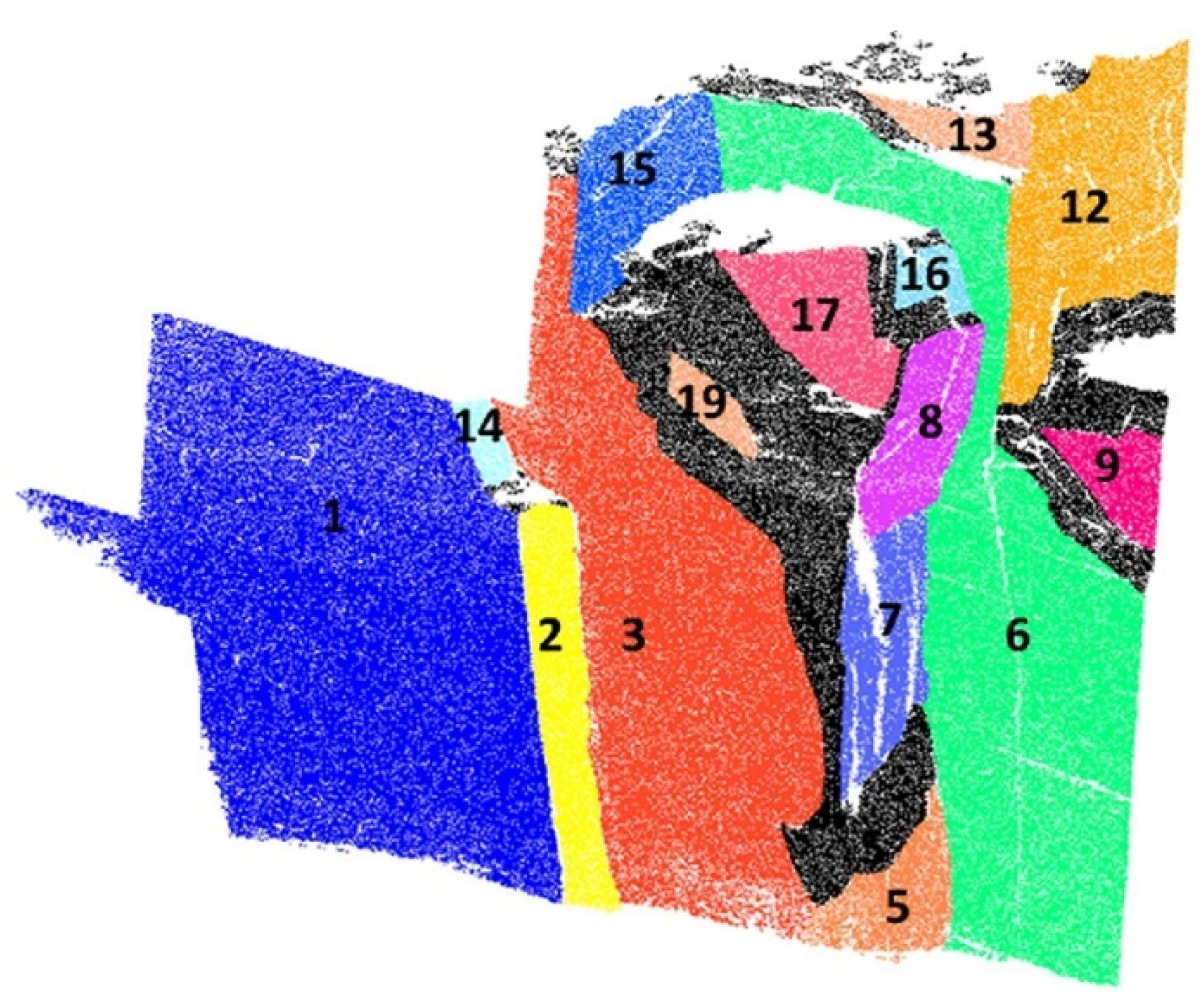Core points, along with all points within the radius $eps$, are grouped into a cluster. This process is repeated for each unprocessed point, ultimately yielding the second-stage clusters that belong to each structural plane. the results of identifying the first set of discontinuities are illustrated in Figure 12.

2.6. Discontinuity Plane Fitting

Given that rock discontinuity surfaces are typically rough and uneven, the orientation of a discontinuity is determined by the orientation of its best-fitting plane. RANSAC is an iterative method designed to estimate surface model parameters from a dataset. It identifies the parameters of a geometric shape by utilizing the smallest number of points needed to define that shape within a point cloud [54,55,56].

It accounts for the variability of the points, offering a more accurate estimation. The RANSAC algorithm is widely applied in shape detection [57,58] and has been effectively used in previous research for plane fitting [34,59].

The RANSAC algorithm repeatedly applies a plane equation to fit the discontinuity, aiming to find the best parameters. The equation for the discontinuity plane is expressed as:

$$Ax+By+Cz+D=0$$

(24)

In this equation, A, B, C, and D are the coefficients, with A, B, and C representing the three components of the plane’s normal vector. D denotes the perpendicular distance from the origin to the plane. The dip angle and dip direction of the planes are determined using Equations (25) and (26).

$$\mathrm{Dip} \mathrm{direction}=\{\begin{array}{cc}{90}^{\circ }-ta{n}^{-1}\left({\displaystyle \frac{B}{A}}\right)& A>0\\ 0^{\circ }& A=0\&B\ge 0\\ {180}^{\circ }& A=0\&B<0\\ {270}^{\circ }-{tan}^{-1}\left({\displaystyle \frac{B}{A}}\right)& A<0\end{array}$$

(25)

$$\mathrm{Dip} \mathrm{angle}=\{\begin{array}{cc}{0}^{\circ }& A^2+B^2=0\\ 90-{tan}^{-1}\left({\displaystyle \frac{\left|C\right|}{\sqrt{A^2+B^2}}}\right)& A^2+B^2\ne 0\end{array}$$

(26)

2.7. Qualitative Segmentation Results

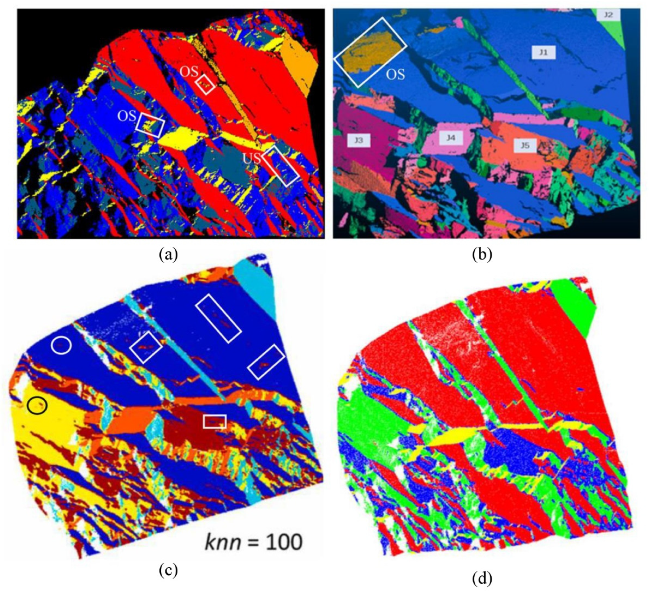
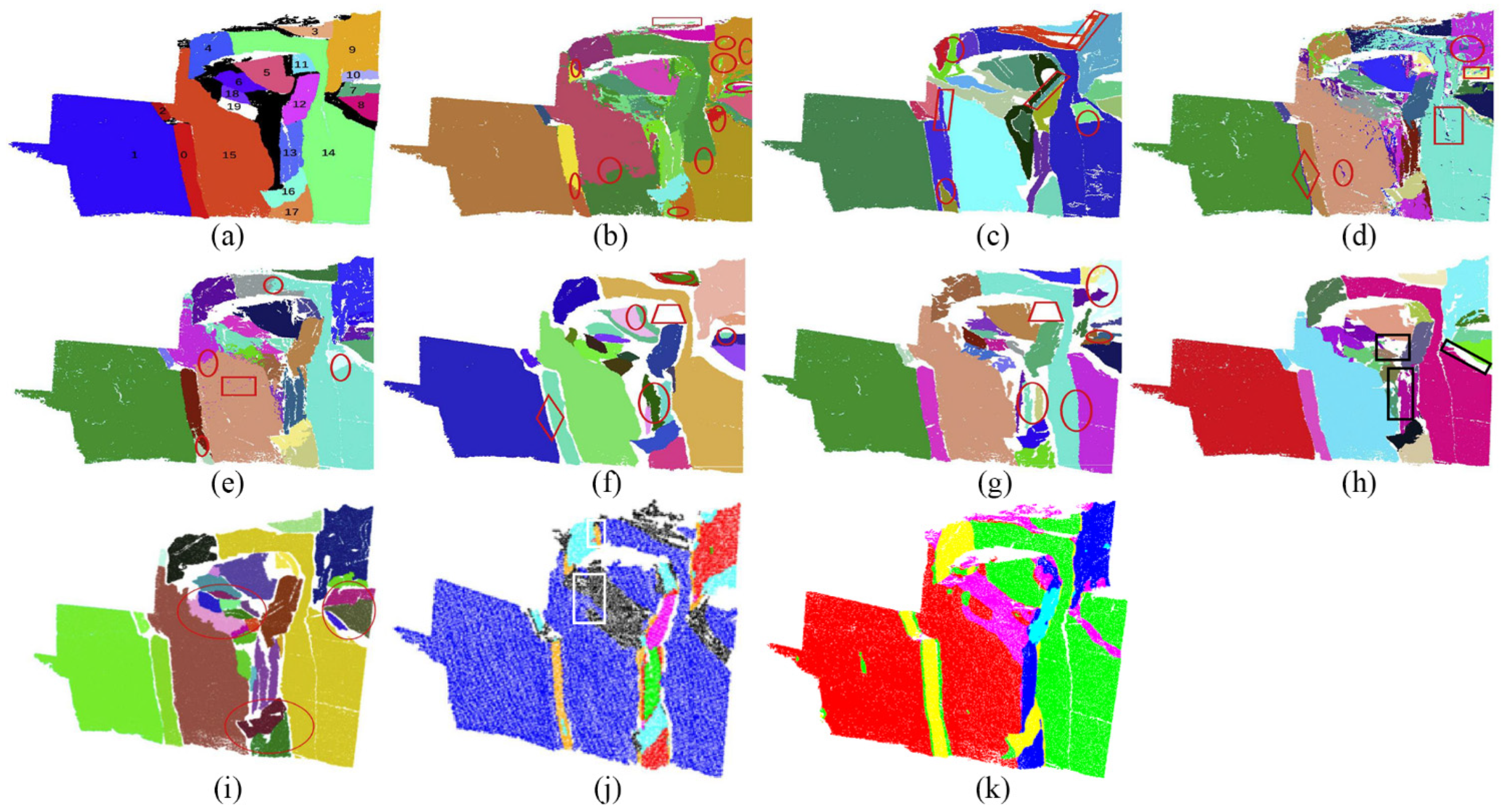
Daghigh et al. [39] reviewed the experimental findings of reference [60] and reference [25], highlighting various examples of deficiencies associated with rectangles and identifying the type of deficiency (OS: over-segmentation; US: under-segmentation) (Figure 13a,b). To optimize segmentation results, Daghigh et al. [22] modified the KNN value and utilized VG downsampling to reduce the surface variation in the point cloud. Nevertheless, certain discontinuities with undulations or minor offsets remain (as shown in Figure 13c, highlighted by the circled and rectangular areas). The visual segmentation results from these studies, along with the current study, are displayed in Figure 13. It can be seen that the results of the present study (Figure 13d) show an ideal segmentation effect in the areas marked with deficiencies, demonstrating that our method for determining the main discontinuity sets can effectively avoid over-segmentation.

For the extraction results of discontinuity orientations, the experimental dataset used in this study has several sets of true orientation values that have been published by other researchers. Riquelme et al. [53] and Chen et al. [60] manually measured the orientations of several typical discontinuities in this dataset. Daghigh et al. [39] conducted a critical evaluation of these measurements and identified significant errors in the data obtained by Riquelme et al. [53] and Chen et al. [60]. As a result, Daghigh et al. [39] re-evaluated the discontinuity orientations by employing the Segment tool in CloudCompare. This method entails drawing a closed polygon around the points related to a particular discontinuity plane and then using the best-fit plane tool to ascertain the plane’s orientation based on the chosen points. This paper uses these results as the true values for discontinuity orientations. 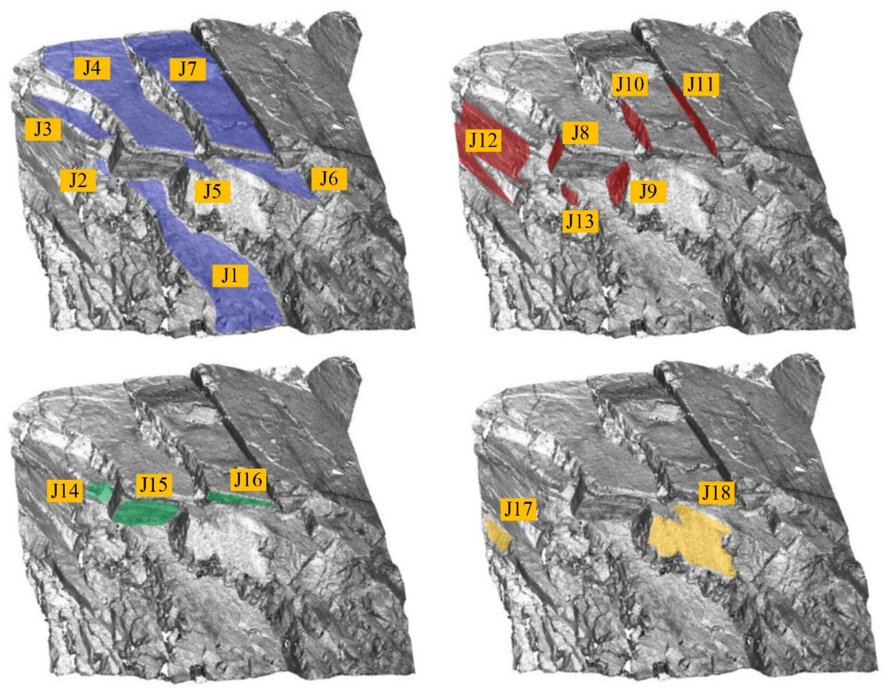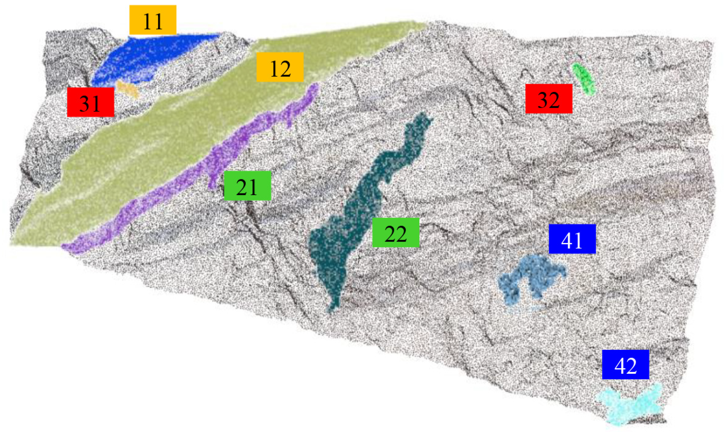Figure 14 shows the numbering of the discontinuities used for comparison, and

Table 3. Comparison of measurement results.

Plane No.	Dip Direction/Dip Angle (°)
	Truth Value (Daghigh et al. (2022)) [39]	Daghigh et al. (2023) [22]	Our Method	Error Degrees
	T	M1	M2	T vs. M1	T vs.M2
1	246.1/39.1	244.93/39.39	244.07/38.54	1.17/0.29	0.86/0.85
2	248.1/49.5	252.77/50.32	243.77/50.45	4.67/0.82	4.33/0.95
3	249.8/35.7	248.95/35.58	249.90/36.06	0.85/0.12	0.10/0.36
4	251.8/34.7	251.85/34.58	251.03/34.07	0.05/0.12	0.77/0.63
5	249.3/35.4	252.89/36.99	248.77/35.23	3.59/1.59	0.53/0.17
6	250.1/35.7	250.45/35.85	250.81/34.95	0.35/0.15	0.71/0.75
7	253.4/33.3	251.22/35.30	253.47/33.36	4.18/2.00	0.07/0.06
8	339.5/83.1	339.67/83.27	338.2/83.61	0.17/0.17	1.30/0.50
9	345.7/73.2	345.19/76.07	163.66/76.12	0.51/2.87	2.04/2.92
10	338.2/88.1	341.02/87.59	338.05/86.83	2.82/0.51	0.15/1.27
11	173.7/76.7	176.47/75.15	174.18/76.23	2.77/1.55	0.48/0.47
12	136.7/77.0	134.40/79.82	315.12/78.54	2.30/2.82	1.65/1.54
13	147.2/89.1	143.66/89.51	147.19/89.21	3.54/0.41	0.01/0.11
14	97.2/62.2	99.55/61.63	101.01/64.73	2.35/0.57	3.81/2.53
15	92.5/48.6	92.28/48.99	93.13/47.52	0.22/0.39	0.63/1.08
16	97.7/48.8	97.40/48.17	97.57/47.82	0.30/0.63	0.13/0.98
17	304.4/77.9	307.35/73.42	304.33/79.63	2.95/4.48	1.22/1.73
18	286.7/70.7	286.72/69.86	286.41/69.30	0.02/0.84	0.29/1.40
Average				1.82/1.69	1.06/1.01

compares the measurement results of our method with those of reference [22] and the true values. It can be observed that our method has smaller errors compared to reference [22], validating that our method provides satisfactory characterization results.

3. Case Studies and Discussion

3.1. Case Dataset

To illustrate the proposed methodology, two case studies of rock slopes were analyzed. In Case A, data were gathered in Kingston, Ontario, Canada, using a Leica HDS600 scanner (Figure 15a). Figure 15b presents the corresponding trimmed point cloud (C1), which comprises 387,610 points with an average spacing of about 4 cm. Case B: A rock slope in a quarry in Wuhan, China (Figure 15c). Figure 15d shows the corresponding trimmed point cloud (C2), consisting of 266,294 points with an average point spacing of approximately 3 cm.

3.2. Case A

For C1, to effectively evaluate the segmentation results, Hu et al. [41] generated a colored ground truth point cloud. This ground truth was later revised by Daghigh et al. [22] and utilized as a benchmark for evaluating the segmentation outcomes (Figure 16). Therefore, we use this colored ground truth point cloud as the standard for assessing the segmentation results obtained by our method.

Figure 17 illustrates the results of employing the watershed-like algorithm to identify non-planar areas in C1. It is evident that the non-planar regions detected by the proposed method encompass those identified in Figure 17, while also revealing additional details. This indicates that the method is effective in accurately identifying non-planar areas.

Figure 18 is the comparison of discontinuous surface segmentation results. Figure 18a shows the color-coded ground truth point cloud. Figure 18b–g illustrate the segmentation results for several typical methods from Liu et al. [61], with red polygons used to emphasize the shortcomings in each outcome. The ellipse marks areas of over-segmentation, the rectangle indicates discontinuities, the parallelogram highlights incorrect results, the rhombus shows poor boundary definitions, and the trapezoid identifies missed detections [61]. Figure 18h,i is the segmentation results of MOE [61] and Supervoxel-RG [42] on C1, as summarized in reference [39]. It can be observed that MOE shows gaps in non-planar areas (marked with black rectangles), while Supervoxel-RG exhibits over-segmentation in non-planar areas (indicated by red ellipses). Reference [22] proposed an improved method and applied it to C1. As depicted in Figure 18j, this approach somewhat mitigates over-segmentation, proving most effective for large-area planes (such as blue and some red planes). For non-planar areas with high curvature, this method can still result in incorrect segmentation (marked with white rectangles). Figure 18k shows the segmentation results of this method on C1. It can be observed that the results align well with the color ground truth point cloud shown in Figure 18a. Additionally, in areas marked by red ellipses, where over-segmentation was prone to occur, the segmentation performance is improved, demonstrating the method’s high segmentation accuracy and its effectiveness in mitigating over-segmentation.

3.3. Case B

Figure 19 shows the recognition results of the watershed-like algorithm. We computed segmentation results for different bandwidths (Figure 20). Analysis reveals that for flat discontinuities (the blue areas in the figure), the best segmentation result is achieved when bandwidth = 0.24. For non-planar areas (the red areas in the figure), a bandwidth of 0.3 results in clearly defined and complete boundaries of the identified point sets with almost no over-segmentation. Therefore, we use 0.24 and 0.3 as the bandwidths for flat discontinuities and non-planar discontinuities, respectively.

Figure 21a shows the final discontinuity surface recognition results. By analyzing the 2D profiles of two typical non-planar discontinuities (as shown in Figure 21c), it can be observed that their spatial distribution approaches a plane, and the segmentation results meet expectations. Figure 21b provides a spherical projection of the characterization results, which includes four discontinuity groups and a total of 51 discontinuities.

To validate the accuracy of the results, we measured the directions using CloudCompare. Figure 22 shows the eight sample planes used for verification (two from each discontinuity concentration), and

Table 4. Comparison of the measurement results between our method and CloudCompare.

Plane No.	Dip Direction/Dip Angle (°)
	Our Method	CloudCompare	Error Degrees
11	14.9/37.5	15.3/37.1	0.4/0.4
12	12.2/40.1	12.1/40.5	0.1/0.4
21	331.1/61.7	329.2/59.5	1.9/2.2
22	318.6/66.3	320.1/67.9	1.5/1.6
31	178.5/77.8	176.5/76.3	2.0/1.5
32	187.1/78.1	185.9/78.9	1.2/0.8
41	358.0/85.5	358.3/84.1	0.3/1.4
42	318.4/80.6	316.6/79.9	1.8/0.7
Average			1.2/1.1

compares our method with CloudCompare measurements. The average errors in dip direction and dip angle for the eight sample planes are 1.2 and 1.1, respectively, indicating that our method has good applicability.

3.4. Computation Time Comparison

Numerous scholars have conducted experiments on the dataset used in this study and recorded the runtime.

Table 5. Run-time comparison.

References	Input	Programming	Computer System	Time (min)
Riquelme et al. (2014) [54]	3D points	MATLAB	Intel Core i3-350 M and 8 GB DDR3 RAM	88
Chen et al. (2016) [36]	2.5D points	Not reported	Intel Core i7-2600 CPU and 16 GB RAM	150
Kong et al. (2020) [1]	3D points	Not reported	Intel Core i5 6300Q and 4 GB RAM	330
Daghigh et al. (2023) [3]	3D points	Python	Intel Core i7-8565U CPU and 16 GB RAM	4
Our method	3D points	Python	Intel Core i7-1195G7 CPU and 16 GB RAM	6

compares the computation time of the proposed method with the runtime of methods proposed by other researchers. The results indicate that the proposed method has a faster runtime, which meets the needs of practical engineering applications. It is important to note that the runtime of a method can be influenced by various factors, such as computer hardware, the programming tools employed, and the complexity of the method. Therefore, the runtimes summarized in Table 5 should not be considered the sole criterion for evaluating the efficiency of a method.

As observed in Table 5, our method takes two minutes longer than the method proposed by Daghigh et al. [3]. Upon analysis, it was found that the most time-consuming part of our method is the process of identifying the main discontinuity sets. The identification of non-planar areas has somewhat reduced efficiency; however, considering its contribution to optimizing the segmentation results, the additional time consumed by this step is acceptable.

4. Conclusions

This paper primarily investigates the problem of discontinuity characterization in unstructured point clouds of rock masses. To address the issue of over-segmentation that often arises when characterizing complex rock mass discontinuous surfaces, a new method based on laser point cloud data is proposed. The method is divided into five main stages: (1) adaptive resampling; (2) normal vector calculation; (3) determination of the main discontinuity sets; (4) recognition of single discontinuity cluster; and (5) discontinuity plane fitting.

The primary novel contributions of the proposed work are: (1) adaptive resampling of point cloud data based on density ratios, which has the capacity to process datasets with varying densities; (2) the watershed-like algorithm can identify the non-planar areas on the rock mass surface; (3) proposed MTMS, which includes a trigger-based bandwidth allocation mechanism, effectively avoiding over-segmentation in non-planar areas (4) accurate calculation of the orientation of discontinuities; (5) fewer critical hyperparameters require adjustment compared to other methods.

To verify the reliability of the results, we applied this method to three real rock mass datasets and compared it with previous research results and manual measurements. For the experimental dataset, it can be seen that the results of the present study achieve satisfactory segmentation in the set of marked deficiency areas, demonstrating that our method for determining the main discontinuity sets effectively avoids over-segmentation. When comparing the extracted discontinuity orientations from this dataset with the ground truth published by other researchers, our method shows smaller errors. For Case A, the identification results from our method align closely with the color-coded ground truth point cloud. Moreover, in areas previously recognized by scholars as prone to over-segmentation, our method provides better segmentation results, proving its high accuracy and effectiveness in mitigating over-segmentation. Furthermore, we validated our method on Case B by comparing the computed discontinuity orientations with measurements from CloudCompare. The average errors for the dip direction and dip angle across eight sample surfaces were all within 2°, indicating good generalizability of our method. We also analyzed the computational efficiency of our method by comparing its computation time with several representative methods on the same dataset. The results demonstrate that our method has a satisfactory computational efficiency, meeting the practical needs of engineering applications, especially for complex rock masses with many non-planar areas.