Ranking of 10 Global One-Arc-Second DEMs Reveals Limitations in Terrain Morphology Representation

Abstract

At least 10 global digital elevation models (DEMs) at one-arc-second resolution now cover Earth. Comparing derived grids, like slope or curvature, preserves surface spatial relationships, and can be more important than just elevation values. Such comparisons provide more nuanced DEM rankings than just elevation root mean square error (RMSE) for a small number of points. We present three new comparison categories: fraction of unexplained variance (FUV) for grids with continuous floating point values; accuracy metrics for integer code raster classifications; and comparison of stream channel vector networks. We compare six global DEMs that are digital surface models (DSMs), and four edited versions that use machine learning/artificial intelligence techniques to create a bare-earth digital terrain model (DTM) for different elevation ranges: full Earth elevations, under 120 m, under 80 m, and under 10 m. We find edited DTMs improve on elevation values, but because they do not incorporate other metrics in their training they do not improve overall on the source Copernicus DSM. We also rank 17 common geomorphic-derived grids for sensitivity to DEM quality, and document how landscape characteristics, especially slope, affect the results. None of the DEMs perform well in areas with low average slope compared to reference DTMs aggregated from 1 m airborne lidar data. This indicates that accurate work in low-relief areas grappling with global climate change should use airborne lidar or very high resolution image-derived DTMs.

1. Introduction

The Shuttle Radar Topography Mission (SRTM) flew in 2000 and began releasing a near-global 3-arc-second (about 90 m) digital elevation model (DEM) starting in 2004 [1]. The quality and free availability greatly surpassed what was available almost universally. Almost every discipline dealing directly or indirectly with solid earth surface morphology has used SRTM data, and 20 years after the first release of data Google Scholar reports about 140,000 references to SRTM. Indeed, like GPS being used by many when there are now multiple GNSS constellations, for many people global DEM means SRTM.

The SRTM DEM, initially released globally at the 3-arc-second scale, eventually released the entire data set at 1-arc-second scale. Since that time a number of additional global DEMs at that scale have been released, covering the polar regions missed by the space shuttle orbit. These include ASTER [2] and ALOS [3], which used optical sensors, the NASADEM [4] reprocessing of the SRTM data, and TanDEM-X [5,6] and CopDEM [7] with improved radar instruments. While the SRTM may have pushed the technology to achieve its claimed 30 m resolution [8], ALOS, TanDEM-X, and CopDEM are downsampled versions of higher-resolution commercial DEMs. All of these DEMs are digital surface models (DSMs), with limited but varying ability to penetrate the vegetation canopy. Our goal in comparing these DEMs is to help users to choose the best DEM for their purpose, and to understand the limitations of all of these 1-arc-second DEMs.

Because many applications for DEMs should use a bare-earth digital terrain model (DTM), a number of hybrid DEMs have appeared using machine learning to remove vegetation from CopDEM. These include FABDEM [9,10], CoastalDEM [11], DiluviumDEM [12,13], and DeltaDTM [14,15]. The validation for these DTMs considered only elevation comparisons.

Many papers have compared some of these DEMs in particular regions, with most comparing only elevations at a small number of points [16]. Bielski and others [17] highlighted the diversity of previous methods developed over time. SRTM started a revolution in modeling Earth’s topography, and later DEMs have built on that legacy.

The Digital Elevation Model Intercomparison Exercise (DEMIX) compared six of these 1-arc-second DEMs [17]. They considered all 140,000 points in their test tiles and looked beyond just elevation and considered slope and roughness, commonly used characteristics derived from the DEM. In this paper, we seek to rank ten DEMs, and improve on the earlier analysis with an order of magnitude more test sites, while adding additional test criteria. Our major new test criterion, the fraction of unexplained variance (FUV), compares the DEM or a derived grid to a reference at the same resolution derived from much higher-resolution lidar data and uses tens to hundreds of thousands of points. In comparing the edited DTMs with DSMs, we highlight some of the limitations of machine learning hallucinations, which decrease DEM capabilities for derived grids that were not part of its training. Improving elevation error rates does not necessarily improve other products derived from the DEM.

In addition to ranking the DEMs, we show where all of these DEMs poorly represent the terrain in low-slope regions, and that the different DEMs behave differently in very steep mountainous regions. Finally, we rank the derived geomorphometric grids in terms of their agreement with reference DEMs, and thus, the amount of skepticism warranted by users in interpreting those grids.

2. Materials and Methods

2.1. Test DEMs

The first DEMIX comparison [17] used six DEMs, five of which were DSMs (CopDEM [7], ALOS [3], SRTM [1], NASADEM [4], and ASTER [2]) and one that was edited to create a DTM (FABDEM [9,10]). Detailed summaries of those DEMs are available ([18], their Table 1; [17], their Table VI).

Since the earlier comprehensive comparison of global DEMs [17], three additional DEMs (CoastalDEM [11], DiluviumDEM [12,13], and DeltaDTM [14,15]; refer to

Table 1. Edited DTMs created from Copernicus DEM.

Elevation Band	Edited DTM	License	Source Data	Methods	Validation
FULL: covers entire Earth	FABDEM [9,10]	Restricted	CopDEM	Random forest	Split-sample, lidar, ICESat-2
U120, <120 m, but 1-degree tiles filled	CoastalDEM 3.0 [11]	Restricted	Several recent and advanced global DEMs	Convolutional neural networks	ICESat-2
U80, <80 m	DiluviumDEM [12,13]	Creative Commons Attribution	CopDEM	Decision tree	Local DTMs from airborne lidar in 10 countries
U10, <10 m	DeltaDTM [14,15]	Creative Commons Attribution	CopDEM	Filtering and co-registration	Local DTMs from airborne lidar in 9 countries

) have attempted to create a DTM using CopDEM as the starting point for machine learning. These focus on coastal areas, and unlike FABDEM, that includes all of Earth’s landmass, they have different cutoffs in terms of the maximum elevation included. Although FABDEM was not specifically calibrated for floodplain/coastal areas, it did prioritize checking in floodplain areas. We thus have 4 elevation categories for the elevation range of the global one-arc-second DEMs: FULL for the entire range of Earth, U120 (limit 120 m), U80 (limit 80 m), and U10 (limit 10 m) (Table 1). When we refer to the U80 data, for instance, these data include not only DiluviumDEM but the reference DTMs and other test DEMs in higher-elevation bands masked to have the same coverage area.

We also include the one-arc-second TanDEM-X [5,6], which has also been recently released, but like FABDEM and CoastalDEM requires a restricted user license. Thus, our comparison includes 10 DEMs, but as will be clear in later sections, the limited elevation ranges of three of the edited DTMs limits where they can be compared. Comparisons are most limited for DeltaDEM, as there are few areas under 10 m elevation, and the legacy DEMs with integer vertical resolution (SRTM, NASADEM, and ASTER) have only 10 possible elevation values within that elevation range.

2.2. Pixel Origin Models

Except for NASADEM, which uses its own nonstandard HGT format and whose only metadata is the file name, all of the global one-arc-second DEMs use the GeoTIFF file format. Previous work [17,18] emphasized the importance of the pixel-is-point and pixel-is-area representations of DEMs, noting that ASTER was anomalous. The difference is critical because pixels cannot be directly compared if they use different geometric representations. In flat areas, the half-pixel offsets generally make little difference, but in steep areas the changes due to the shift become substantial. The GeoTIFF encoding for these DEMs does not indicate how the data were sampled but only describes the geometry of the pixel. The complexity of data sampling cannot be easily encoded in a simple numeric code.

Because CoastalDEM and ALOS test DEMs now use the same approach, the concept of the pixel origin model appears to be a better approach than the pixel-is-area or pixel-is-point. We propose naming the two approaches the SRTM and ALOS geometries, after the first freely available global DEMs using that model. GIS and remote sensing software use the centroid of the pixel for computations; even Landsat satellite data, clearly sampled as pixel-is-area, use pixel-is-point [19]. One-arc-second DEMs use one-degree tiles, named for the SW corner, with minor exceptions (e.g., USGS 3DEP names for the NW corner and includes a buffer, so the nominal corner is not the actual corner). If the nominal corner of the cell is the centroid of a pixel, the pixel origin model is SRTM; when the nominal corner is a pixel corner, the model is ALOS. The pixel origin model is unambiguously encoded in GeoTIFF files in two tags, GTRasterTypeGeoKey (#1025) and ModelTiepointTag (#33922).

Table 2. DEM pixel origin models.

DEM	Pixel-Is (GeoTIFF Tag #1025)	Model Tie Point (GeoTIFF tag #33922)	Nominal DEM Corner	Pixel Origin Model
CopDEM, TanDEM-X, FABDEM, SRTM, and NASADEM	Point	DEM nominal corner from file name	Pixel centroid	SRTM
ASTER and CoastalDEM	Area	Half-pixel offset from DEM nominal corner	Pixel centroid	SRTM
ALOS, USGS 3DEP and DiluviumDEM	Area	DEM nominal corner from file name	Pixel corner	ALOS

shows how this has been applied to global one-arc-second DEMs, and while other models for the pixel origins could be developed, we have not seen them actually used.

Comparing DEMs with different pixel origins requires either resampling or reinterpolation. Many programs have required reinterpolation to UTM to use simpler equations for computations like slope, but all computations can be performed in geographic coordinates [20,21]. Comparison could reinterpolate both DEMs to a common projected coordinate system to match comparison points, or reinterpolate one of the DEMs to remove the half-pixel offset to the other DEM. In order to compare the DEMs without interpolation introducing differences, we create separate reference DTMs in both pixel origin models.

At higher latitudes all of the edited DTMs use a one-arc-second horizontal grid spacing, interpolating from the larger spacing used by CopDEM and TanDEM-X. Some options for obtaining CopDEM also resample the higher-latitude data, and users of that data should understand the implications.

2.3. Test Areas

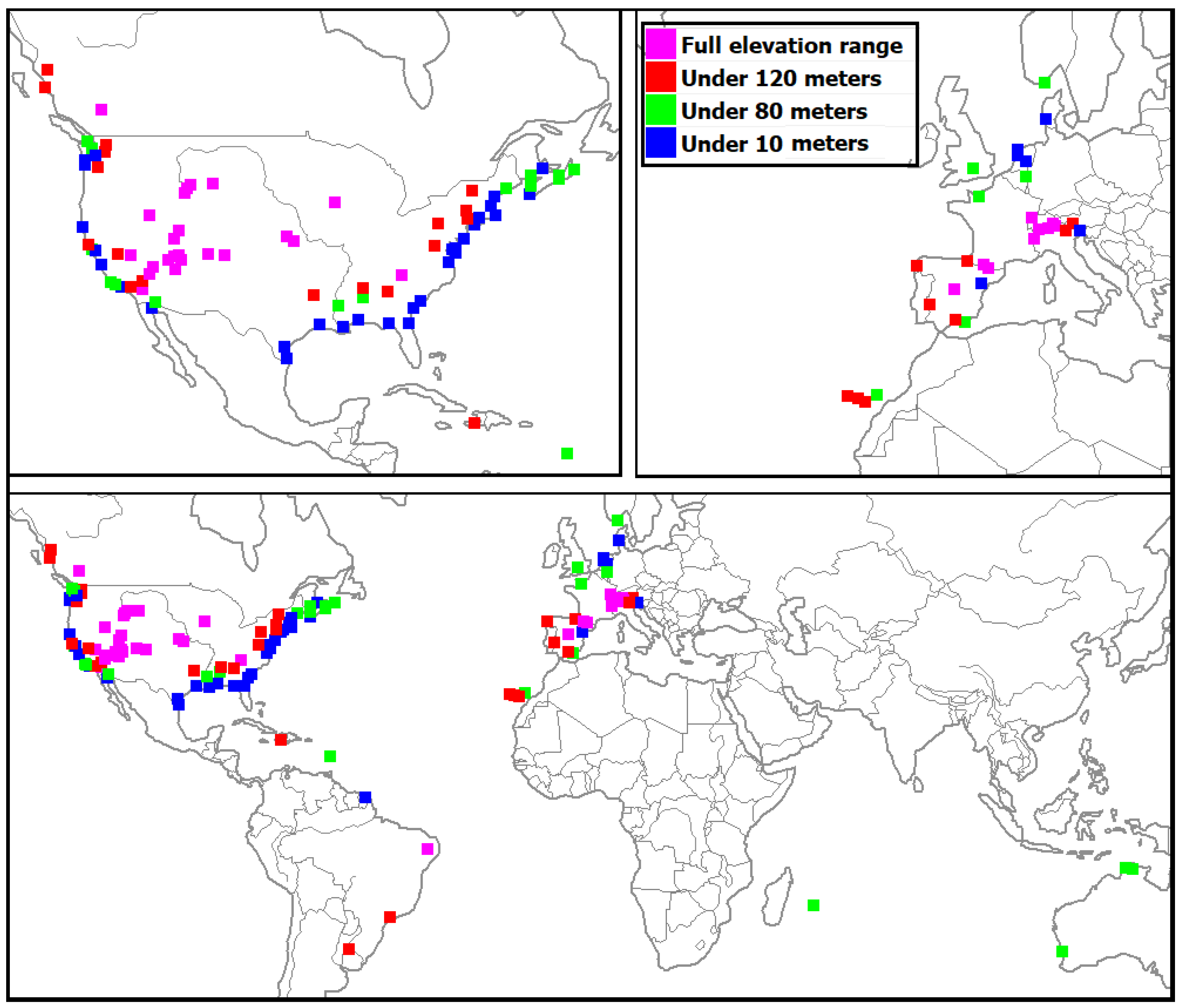
Our full data set has 124 test areas and 3462 DEMIX tiles, each approximately 10 km × 10 km [22]; the first DEMIX comparison [17] had 24 test areas made up of 236 DEMIX tiles. Figure 1 shows the location of the test areas in our greatly expanded data sets. The availability of free lidar DTMs skews our sampling to western Europe and North America, but the variety of landforms should be representative of most of the world. To perform a valid comparison with the U120, U80, and U10 edited DTMs, we deliberately over-represented coastal areas.

Our selection of test areas was guided by the ease of downloading terabytes of source data and the need for diverse landscapes (

Table 3. Distribution of test areas and DEMIX tiles by country.

Country	Test Areas	DEMIX Tiles
United States	71	2139
Spain	12	346
France	7	243
Italy	3	214
Switzerland	4	118
Haiti	1	116
Canada	10	92
UK	1	51
Australia	3	34
Netherlands	4	20
Denmark	1	11
Brazil	2	9
Norway	1	3
Uruguay	1	1

). The United States dominates the test suite because of the high quality of the 3DEP data from the USGS [23]. We deliberately sampled several other areas (French Guyana, Haiti, and Australia) to expand the range of landscapes available. The nature of the GIS database would allow repeating the analysis to exclude data sets to confirm the validity of results. Most of the source DTMs have 1 m resolution, but the metadata for the database [24] has the resolution for each test area, which ranges from 0.25 to 5 m.

2.4. Comparison Criteria

We computed grids using MICRODEM [25,26], WhiteboxTools [27,28], Whitebox Workflows [29], and SAGA [30]. Calls to WhiteboxTools and some SAGA tools are integrated directly in MICRODEM, whereas we used Jupyter notebooks for Whitebox Workflows and some SAGA tools. Several of the Whitebox Workflows options required a license, and Whitebox Workflows more efficiently processes options that require computing multiple intermediate grids than does WhiteBox Tools. Grid comparisons and final statistical work to create the database was performed in MICRODEM. Source code for MICRODEM and the Jupyter notebooks is posted on GitHub [26].

All of the computations use every pixel in the DEM within the DEMIX tile and compare it to the result from a reference DTM downsampled from much higher resolution lidar DTMs, generally with 1–2 m resolution and at most 5 m resolution. The criteria belong to four different computing categories, which we put in four separate tables.

We improved the earlier methodology [17] by masking out water areas, computed from 100 m land cover [31], before computing statistics so that lakes and coastal areas do not bring down computed values like average slope. The DEMIX tiles were designed to have relatively constant areas, but in many test areas some tiles have missing data due to coast lines, political boundaries, or mapping project edges. Because one of our goals was to compare the edited coastal DEMs, we also lowered the percentage of the DEMIX tiles that had to have valid elevations from 75% to 25%, which still leaves at least 35,000 values to compare in each tile and increases the number of coastal tiles we can compare.

We use the term “evaluation” for the floating point numerical result of applying a criterion to a particular test/reference DEM pair. We use “rank” for the ordering of the evaluations of the test DEMs for a criterion. The ranks start as integers, but adjustments for ties due to tolerances for imprecision in the evaluations lead to floating point values. The ranks always go from a minimum of 1 to a maximum for the number of test DEMs considered. Averaging ranks for many criteria or tiles also leads to floating point ranks.

2.4.1. Statistical Measures from the Difference Distribution

The 15 criteria used ([17] Section II-E) improve on traditional metrics in several important ways. First, instead of a handful of known elevations, they use tens of thousands of comparison points. Second, the use of metrics for the slope and roughness difference distribution recognizes that derived grids can be as important as the elevation values, and that the accuracy of metrics from the derived grids does not necessarily correlate with the elevation grid accuracy. The values of these metrics vary with the relief, slope, and ruggedness in the tile, making it hard to compare evaluation values from dissimilar tiles.

2.4.2. Fraction of Unexplained Variance (FUV)

We computed FUV metrics for a wide array of 17 geomorphometric grids (

Table 4. New comparison criteria.

Criterion	Meaning	Computing Category	Geomorphometric Category	Computation Area	Additional Grids Required	Algorithm	Computation Software
ELEV	Elevation	Grid FUV	Grid value	Single grid cell		N/A	N/A
SLOPE	Slope	Grid FUV	First derivative	3 × 3 neighborhood		[34]	MICRODEM
TPI	Topographic position index	Grid FUV	First derivative	7 × 7 neighborhood		[35]	MICRODEM
HILL	Hillshade	Grid FUV	Perceptive index or First derivative	3 × 3 neighborhood		Originally based on [36]	MICRODEM
OPEND	Downward openness	Grid FUV	Perceptive index	8 radials out to 250 m		[37]	MICRODEM
OPENU	Upward openness	Grid FUV	Perceptive index	8 radials out to 250 m		[37]	MICRODEM
RUFF	Roughness (standard deviation of slope)	Grid FUV	Second derivative	5 × 5 slopes (7 × 7 elevations)		[38]	MICRODEM
RRI	Radial roughness index	Grid FUV	Second derivative	5 × 5 neighborhood		[39]	MICRODEM
PROFC	Profile curvature	Grid FUV	Second derivative	3 × 3 neighborhood		[20]	WhiteboxTools
TANGC	Tangent curvature	Grid FUV	Second derivative	3 × 3 neighborhood		[40]	WhiteboxTools
ROTOR	Rotor	Grid FUV	Second derivative	3 × 3 neighborhood		[41]	Whitebox Workflows
PLANC	Plan curvature	Grid FUV	Second derivative	3 × 3 neighborhood		[42]	WhiteboxTools
HAND	Height above nearest drainage (elevation above stream)	Grid FUV	Hydrology related	Entire test area	Flow accumulation, streams	[43]	Whitebox Workflows
WETIN	Wetness index	Grid FUV	Hydrology related	Entire test area	Flow accumulation, slope	[44]	WhiteboxTools
LS	Sediment transport (slope length factor)	Grid FUV	Hydrology related	Point and downslope neighbors	Flow accumulation, slope	[45,46]	Whitebox Workflows
CONIN	Convergence index	Grid FUV	Hydrology related	3 × 3 neighborhood		[47]	Whitebox Workflows
ACCUM	Flow accumulation, log transform	Grid FUV	Hydrology related	Entire test area		[48]	Whitebox Workflows
GEOM	Gemorphons	Per-pixel raster classification	Point classification	Local neighborhood		[49]	WhiteboxTools + MICRODEM
IP12	Iwahashi and Pike 12 category classification	Per-pixel raster classification	Point classification	10 cell neighborhood		[50]	SAGA
CHAN_MISS1	Channel network mismatch, 1 pixel wide channels	Vector comparison	Hydrology related	Entire test area		[17]	Whitebox Workflows + MICRODEM
CHAN_MISS3	Channel network mismatch, 3 pixel wide channels	Vector comparison	Hydrology related	Entire test area		[17]	Whitebox Workflows + MICRODEM

), selected as important representatives of the hundreds of land surface parameters [32,33]. The grids contain floating point values on continuous scales. The FUV equals 1 − r², the squared Pearson coefficient, and ranges in value from 0 (best, r² = 1) to 1 (worst, r² = 0). The restricted range of evaluation values allows comparison of different tiles to generalize controls on the performance of one-arc-second DEMs, as well as facilitating the production of graphics showing the relationships present in our databases. The correlation coefficient, r², or FUV are effective ways to compare grids and multiple land surface parameters [33], but their systematic use to evaluate the quality of DEMs with respect to a reference DTM is a novelty of this work.

2.4.3. Landform Raster Classification and Vector Comparisons

Two landform raster classifications from the DEM, geomorphons [49] and Iwahashi and Pike [50], with a limited number of integer categories, assign a code to every pixel. We computed the kappa coefficient, a widely used metric [51] but not without critics [52]. We also computed user accuracy, producer accuracy, and overall accuracy. The four are highly correlated.

Vector comparison of drainage networks, derived from the DEM, previously hinted at the relevance of drainage network extraction for practical applications [17], and we extend the analysis to all the test areas. To minimize edge effects, the channel network is derived for the entire test area, and then, compared in each DEMIX tile.

Our protocol uses DEMIX tiles [22] with nearly constant 100 km² areas. Some of the comparison criteria might more appropriately use a different test area such as drainage basins. Because we want to evaluate the ability of the test DEMs to match output created by a reference DTM of much higher quality, all the test DEMs face the same issues in dealing with a truncated drainage basin. The resulting stream network might misrepresent locations along the boundary, but is expected to be comparable with a network derived from the reference DTM and allow us to compare the test DEMs.

2.5. DEMIX Database Version 3

The new version 3 of the DEMIX database [24] has multiple tables, separated by elevation ranges, and the four computing categories by elevation bands.

Table 5. DEMIX database versions.

Database Table	Data Set	Areas	DEMIX Tiles	Difference Distribution Records	FUV Records	Raster Classification Records	Vector Comparison Records
DEMIX DB v3	Full	124	3462	50,319	58,854	27,603	5838
DEMIX DB v3	U120	69	1569		23,249
DEMIX DB v3	U80	48	727		1041
DEMIX DB v3	U10	26	285		4159
DEMIX DB v2 [17]	Full	24	234	55,699	N/A	N/A	N/A

compares the new database with the older version 2 [53]. The number of records in the database can be estimated as the number of tiles times the number of criteria. Version 2 had additional records for the tiles with a reference DSM and records for each tile using only the pixels meeting land cover or slope criteria, which we ultimately found not to be helpful.

To make better comparison with the edited DTMs created from CopDEM for low-elevation coastal DEMs, our database deliberately over-represents those areas. Users interested in higher-elevation inland areas should understand the implications of our sampling, and filter the database to match the types of terrain types of interest.

There are slightly smaller numbers of records in the raster classification and vector comparison tables because some criteria (notably related to flow accumulation and channel networks) could not be computed in some of the very flat tiles along the coast.

We created multiple separate tables within the database and analyzed each separately for the four DEM elevation ranges and the categories of criteria. For each edited DTM we masked the appropriate reference DTM and other test DEMs so that metrics are computed over the same area. The number of tiles decreases from the FULL elevation range database to the U120, U80, and U10, which are subsets of the FULL elevation range database. The filled percentage of the tiles frequently decreased in the lower subsets so that we reduced the percentage required to 25% to increase the number of tiles for comparison. We also selected more coastal areas to improve the number of comparisons we could make, and they are over-represented.

For version 3 of the database, we only considered a reference DTM, due to the limited availability of reference DSMs and because CopDEM has been proved to perform very well even when compared to a DTM [17]. Faced with no alternatives, many users treat all the global DEMs as if they were a DTM or as if a DTM and a DSM are interchangeable, so it is worth knowing how CopDEM compares to a true DTM. We also did not break down the pixel results by land type because of the limited utility of those distinctions.

3. Results

The ability of a one-arc-second DEM to match the performance of a reference DTM obtained using mean aggregation from a 1 m lidar-derived DEM depends on many factors, most importantly optical versus radar satellite sensors, the slope and roughness of the terrain, and the land cover, including forest, urban, and barren. Throughout the rest of the paper we use five subdivisions of our test tiles: slope under 5%, slope over 5%, slope over 30%, slope over 55%, and barren percentage over 40%. The boundaries are somewhat arbitrary, but demonstrate real changes in the performance of the DEMs, and the database can be filtered to investigate other category boundaries or combinations of factors.

An elevation bias, where the test DEM is consistently high or low, only affects the elevation results. Derived grids that consider a point neighborhood, like slope, remain unaffected. An elevation bias does not affect slope and roughness in the difference distributions [17], all but one of the FUV criteria we will introduce, the raster pixel classification criteria, and the vector mismatch criteria. We argue that relying only on the elevation errors misses many important DEM uses, where the local surface morphology is equally important. Users concerned with accurate absolute elevations, such as monitoring sea level rise or coastal erosion, should consider using a subset of our criteria because most of the criteria do not reflect absolute elevation differences.

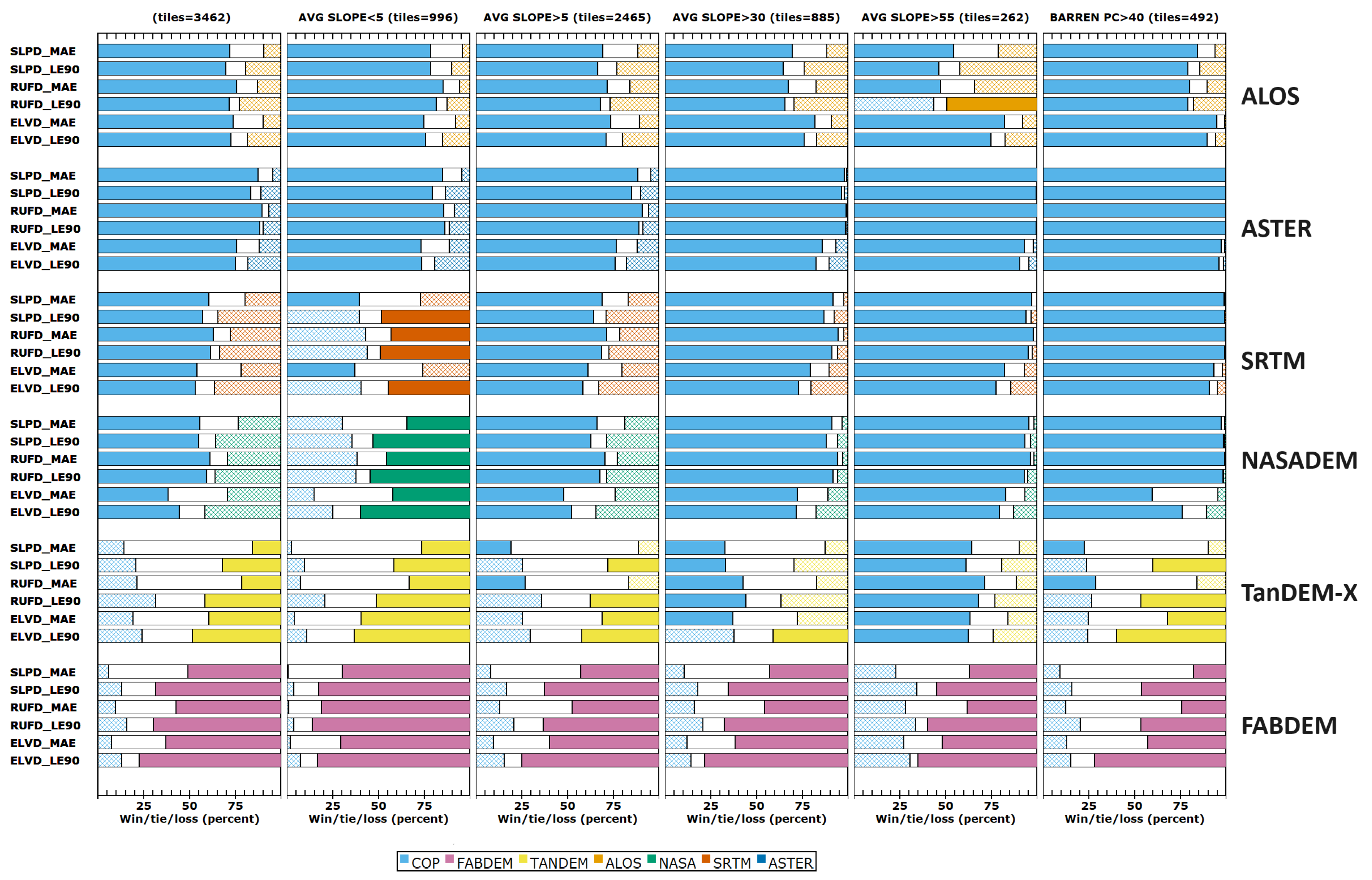
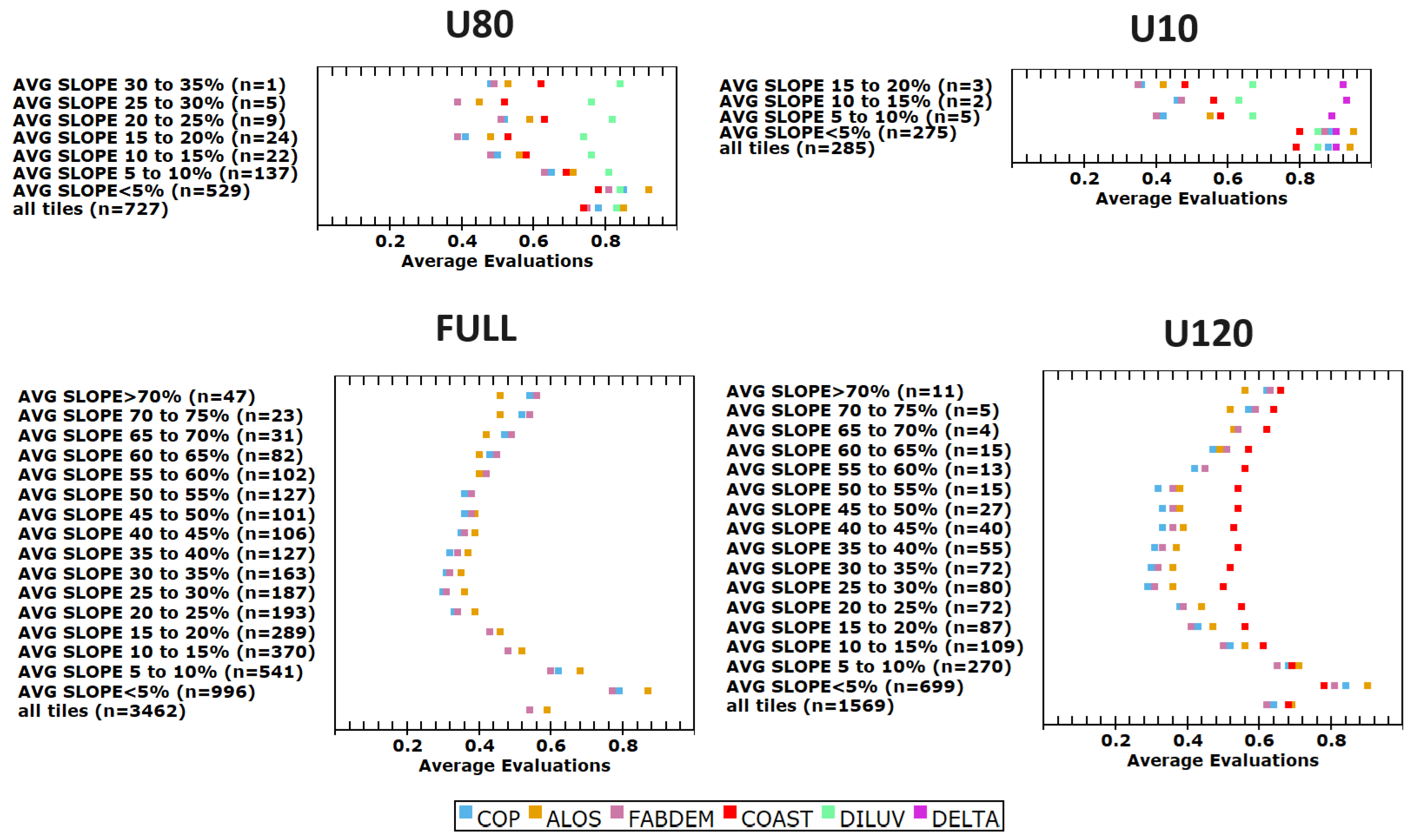
Figure 2 presents the best summary of our results. Each row contains a different set of filters for the database, in terms of the percentage of the tile that is barren or forested, the average roughness, and the average slope. The filter labels also show the number of tiles evaluated that meet the condition. The bottom row in each graph shows the results from the entire data set, and rows above show the series of filters. The column of graphs on the left shows the average ranks using the difference distribution criteria, computed by comparing the evaluations from each criterion [17]. If it were always tied with one other DEM, the DEM would have a ranking of 1.5. That same 1.5 rank could also result if the DEM were the best half of the time and second best the other half of the time. A rank of 7 would mean the DEM was always the worst performing, which is close to ASTER’s results. The only tiles in which ASTER does not have the lowest ranking are those where it ties, because none of the test DEMs match the reference DTM.

The graphs of rankings are similar to Figure 6 in [17], but with an order of magnitude more test tiles and an order of magnitude more landscape filters for the selected characteristics. The middle column of each graph shows the ranks for the new FUV criteria, and the column on the right shows the evaluations that led to the rankings only for the FUV criteria, which is possible because the evaluations all have a common range. The evaluations highlight how close the DEMs were, which the ranks can mask. The design of the wine contest [17] proves sensitive to the tolerances; as soon as two DEMs differ by more than the tolerance, the ranks jumps by one. The evaluations also show how closely the DEM compares to the reference DTM; low values indicate high correlation, and high values low correlation. The graphs for average slope and roughness show that the DEMs compare best to the reference DTM for tiles with moderate slope and roughness. The evaluation graphs would work with a single one of the difference distribution criteria because each has a different range in each tile. The FUV criteria, and the others we introduce in this paper, all have the same limited range of 0 to 1.

3.1. Difference Distributions for FULL Elevation Range

The panels shown in the left column of Figure 2 show the FULL elevation range database. The results for the FULL data set depend on the choice of test areas; as we increased the number of low-elevation tiles along the coast for our evaluation of edited DTMs, these conclusions changed, and we added multiple filters to better explore the controls on the comparisons to the reference DTM. The differences between these results and those in the earlier DEMIX study [17] result from the over-representation of coastal tiles. The best way to eliminate the bias from low-coastal area tiles would be to only consider the tiles with average slopes above 5%.

FABDEM performs better than CopDEM in all the difference distribution criteria for the entire set of test tiles, except for the tiles with the steepest slope and roughest terrain. ALOS performs better than CopDEM in very steep terrain (>55% slope, but this occurs on a continuum), and for high roughness, generalizing previous results from a single area [54]. The poor results for ALOS, both overall and especially for slopes under 5%, indicate that the ALOS DEM performs poorly in the coastal environment. TanDEM-X performs slightly better than CopDEM in a few circumstances.

SRTM and NASADEM very rarely outperform CopDEM, and only for very low slopes. ASTER never outperforms CopDEM, and indeed never outperforms any of the other DEMs. The results for SRTM, NASADEM, and ASTER are true for all comparisons in this study; we show only the better performing DEMs in many of the figures but the full results are in the database [24]. One notable exception is for tiles with very low average slope, where NASADEM and SRTM slightly outperform CopDEM for some criteria. This is something of a Pyrrhic victory, as for low slopes none of the one-arc-second DEMs perform very well.

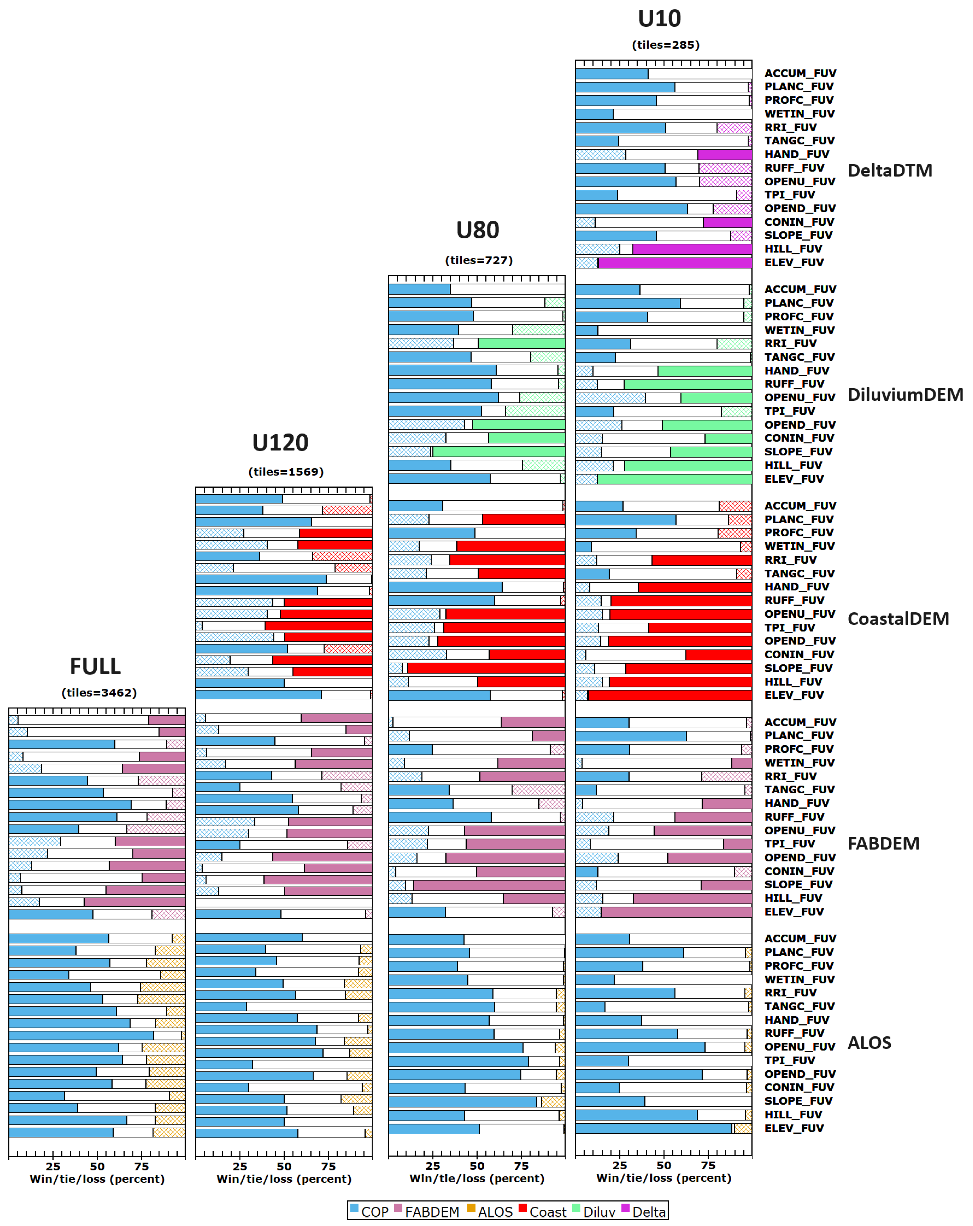
Another way to compare DEMs looks at pairwise comparisons as to how each compares to a reference DTM (Figure 3). CopDEM appears as the leftmost bar in the figures as the base comparison so that the graphs will be similar when we add additional elevation bands with edited DTMs derived from CopDEM. CopDEM has also been widely regarded as the best performing of the one-arc-second DEMs [17,55]. We use the same colors for each DEM throughout this paper; the solid color shows the DEM that wins (has a lower FUV) in more tiles, and the cross-hatch pattern shows the loser for that comparison. At low-resolution versions of the graphs, the cross-hatch pattern appears to be a less saturated version of the solid color. The white zone in the middle shows ties, where the two DEMs are the same within the selected tolerance. Some tolerance is required to deal with floating point arithmetic; we chose the tolerances using the distribution of differences within the database, aiming for a figure with about 10% of the tiles being tied across all the DEMs. The tolerance depends on the criterion; for elevation it is very small and for other parameters much larger. With only five categories, this is less nuanced than the results in Figure 2, but provides a graphic summary and discriminates the differences in criteria behavior.

NASADEM and SRTM perform well only for very low slopes, and ALOS only for very steep tiles. TanDEM-X is close to the performance for CopDEM, and FABDEM performs better in all of these categories, but Figure 2 shows more nuance to that assessment at very large average slope and roughness.

3.2. FUV Criteria

Comparing the different evaluations for the difference distributions is complicated because the magnitudes vary with the terrain, the parameter, and the metric. Our new FUV metric is scaled from 0 (best) to 1 (worst), and makes it easier to compare across both different criteria and different types of terrain.

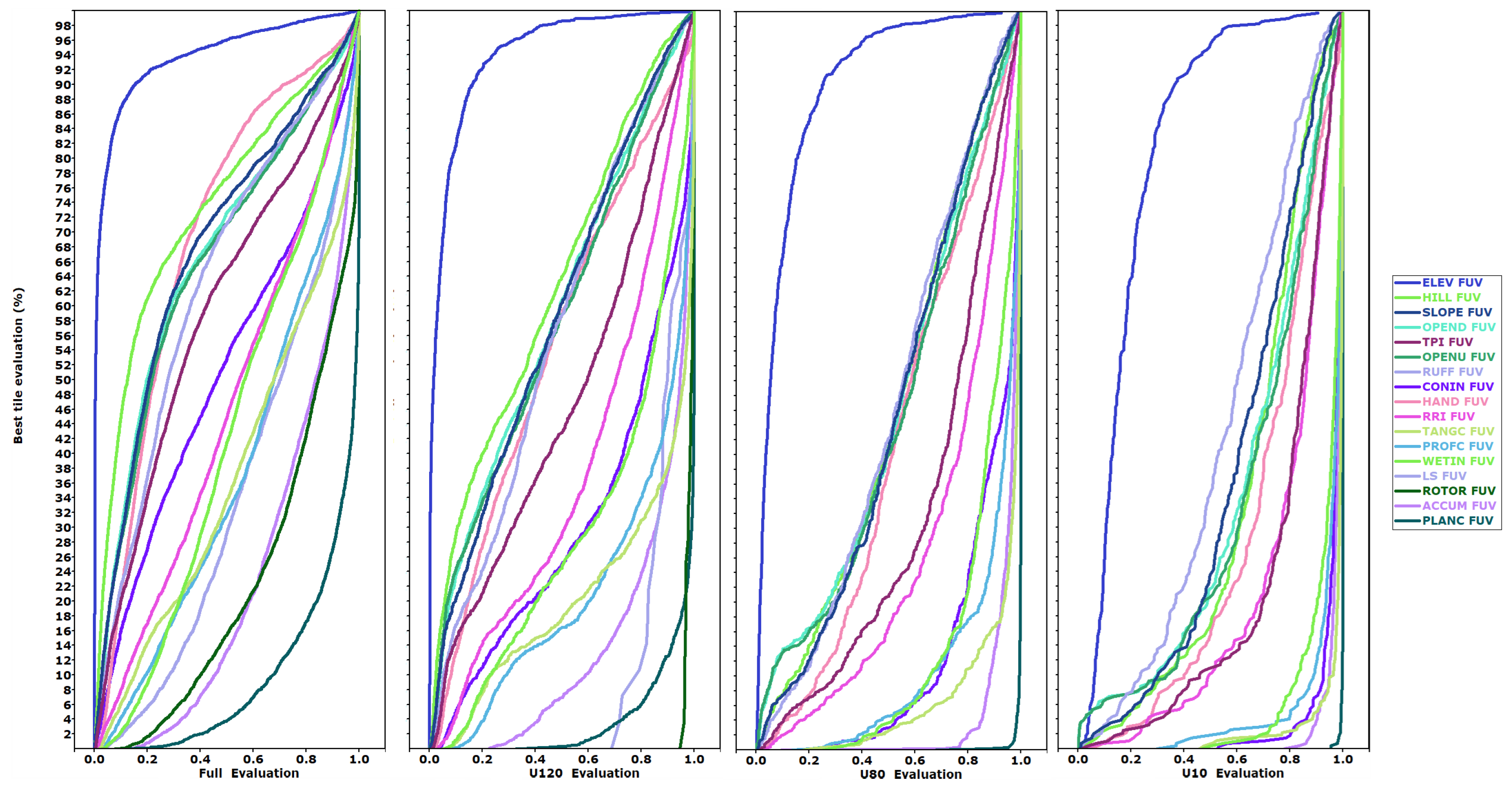
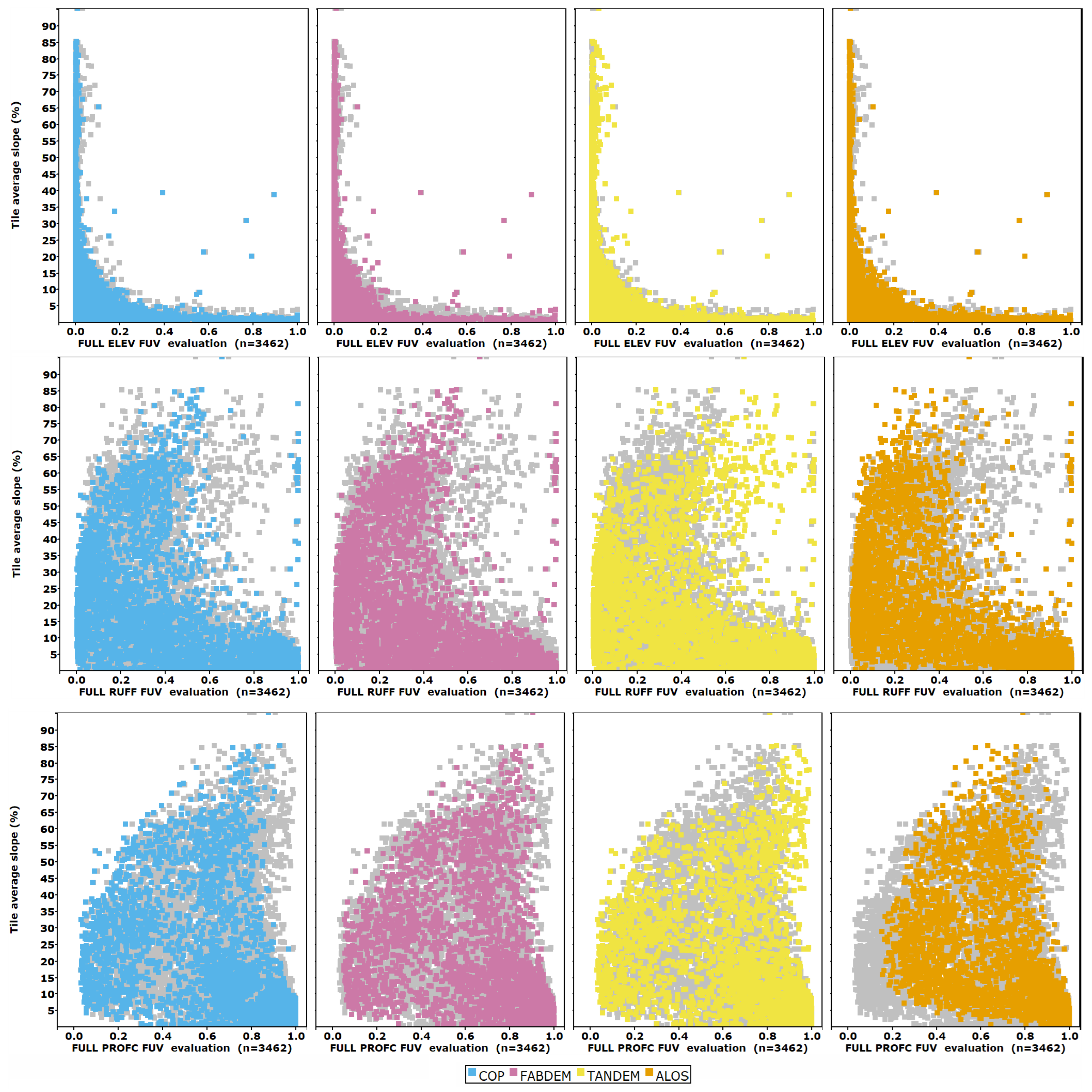
A separate table in the database [24] contains the FUV criteria results. Because those evaluations range between 0 and 1, they cannot be easily combined with the results from the difference distributions. Figure 4 summarizes the database and bears careful scrutiny to understand our efforts to interpret complicated relationships. The FUV evaluations on the x-axis go from 0 on the left, where the test DEMs compare perfectly with the reference DTM, to 1 on the right, where the two are uncorrelated. On the y-axis, we sort by the best evaluation in any of the test DEMs and plot them by percentiles. The 0th percentile has the best match to the reference DTM, and the 100th percentile at the top has the worst. Until about the 50th percentile for elevation FUV, all the DEMs are close to zero—there are very clear, consistent differences, but they do not show up at this scale since the Pearson correlation coefficients are so close to 1. Low FUV values indicate better agreement, thus elevation is clearly the best/easiest criteria to match because the FUV curve is always farthest to the left, often by a wide margin. The legend shows the criteria and the derived grids in the order in which they generally appear, from left to right in the graphs, which indicates how well the test DEMs match the reference DTM for that derived grid. We arrange the panels in order of increasing DEM performance based on the filters, with the best panel on the right. The low-slope tiles appear on the left panel because they consistently have high FUV evaluations. As tile slope increases, the FUV values typically decrease, which is also the case for the most barren tiles.

Second derivatives of elevation (curvature) perform worst, likewise metrics that require calculation of multiple intermediate grids. TPI, essentially a residual DEM obtained from filtering out the trend, is particularly interesting because it can isolate the fine-scale component of spatial variability. This component highlights very well the deterioration in quality of DEMs, including the presence of artifacts. For example, in extreme conditions the correlation between the TPIs of ASTER and the reference DTM can be negative. The two roughness indices behave differently (RUFF is uni-directional and RRI multidirectional) and highlight the potential differences in derived grids that initially appear similar.

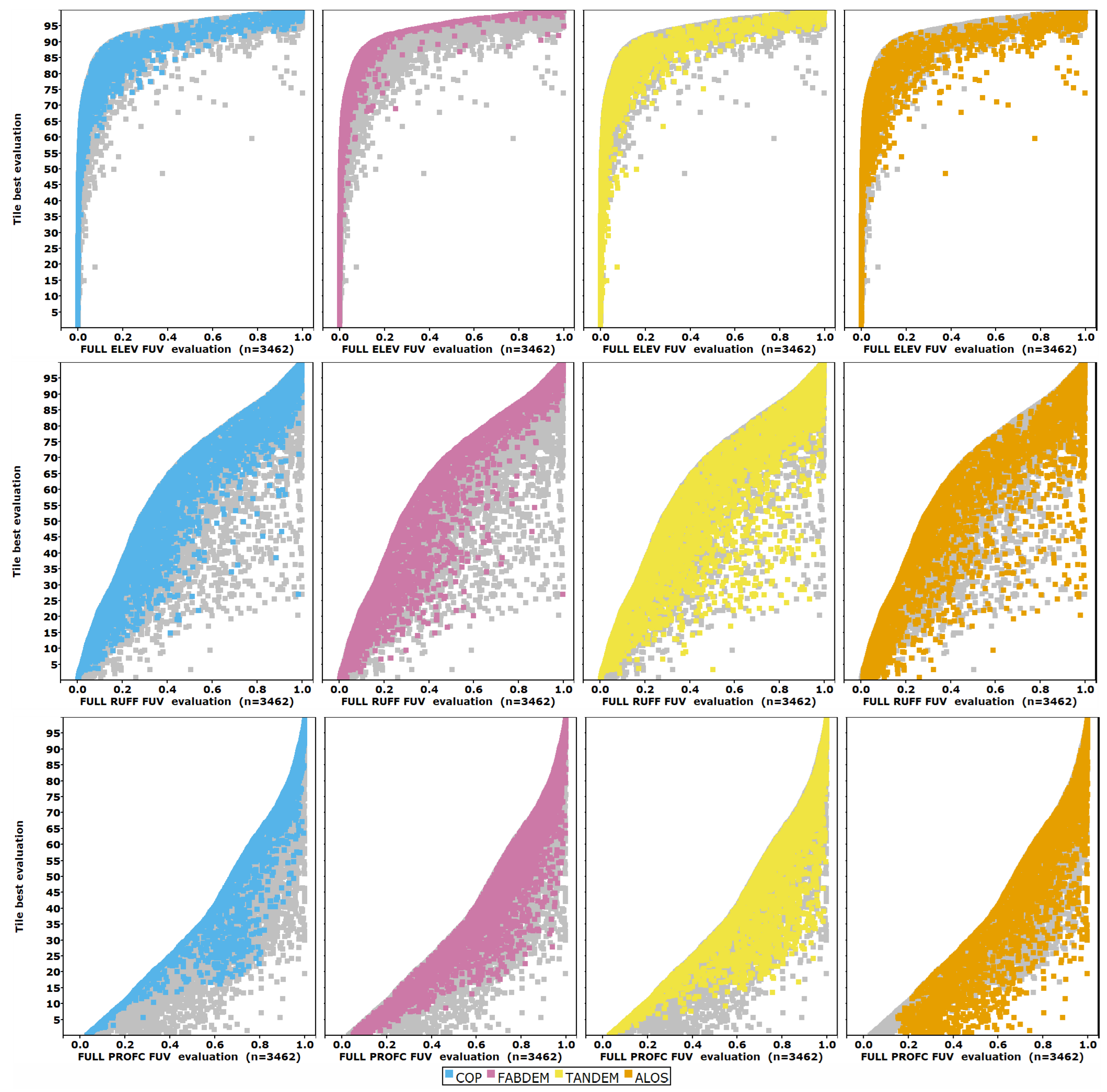
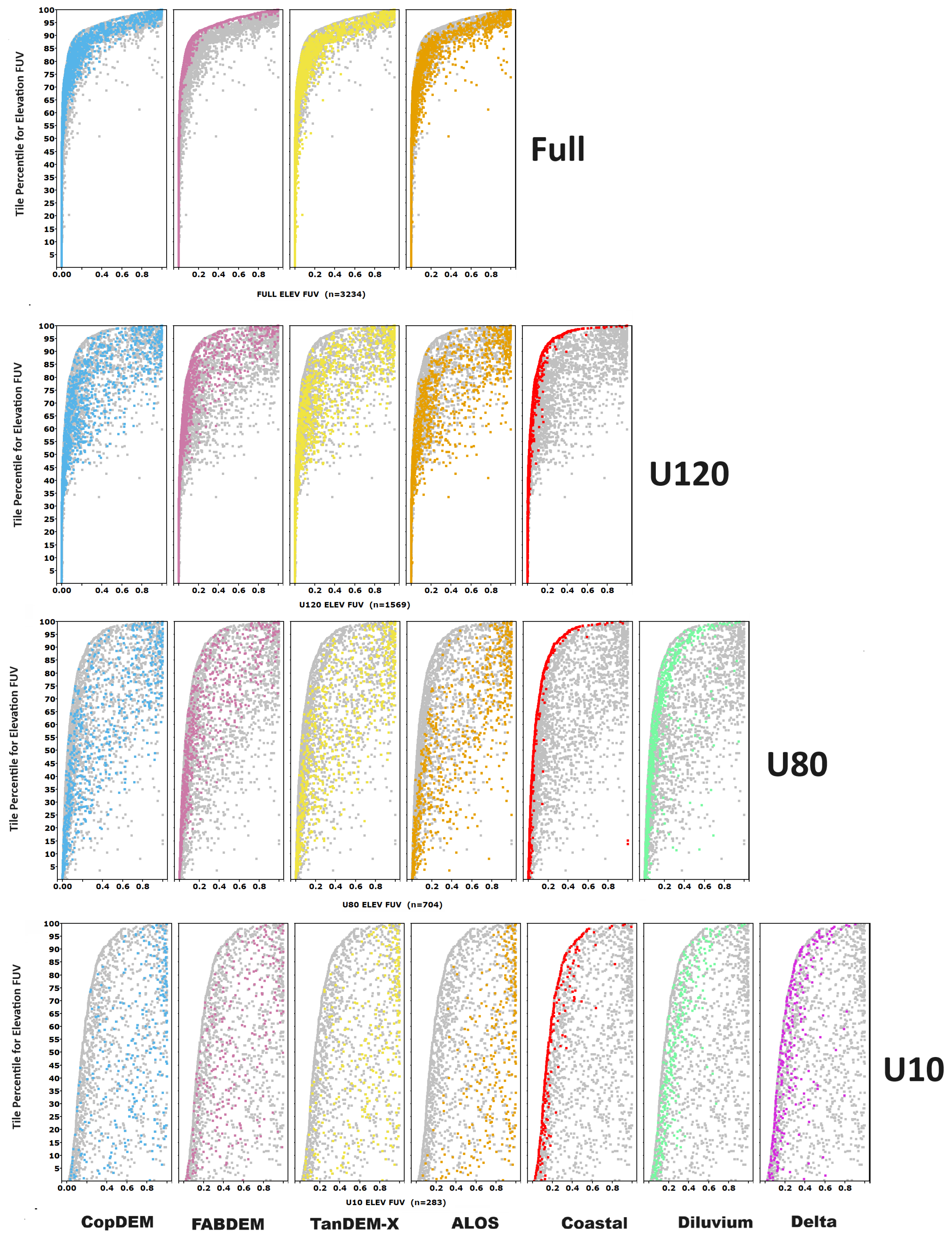
In Figure 5, we show the results by test DEM for all tiles; sorting the plot by the best evaluation reduces noise. The test DEMs that most closely match the reference DTM, with a low FUV evaluation, plot at the bottom left corner of the graph, and those which do not match the reference DTM plot at the top right. To discern the patterns in the FUV criteria results, we plot the FUV on the x-axis. Roughness and profile curvature have lower values of FUV at all percentiles. We only show the data for the best DEMs (CopDEM, FABDEM, TanDEM-X, and ALOS); data for the others are included in the database [24] and in some summary graphics. The three criteria shown include one in the lower range but not the worst performing (profile curvature), one in the central group (roughness), and the best (elevation). More than 3200 files are on the plot, with each colored DEM in a separate panel, with the gray background points showing the other DEMs.

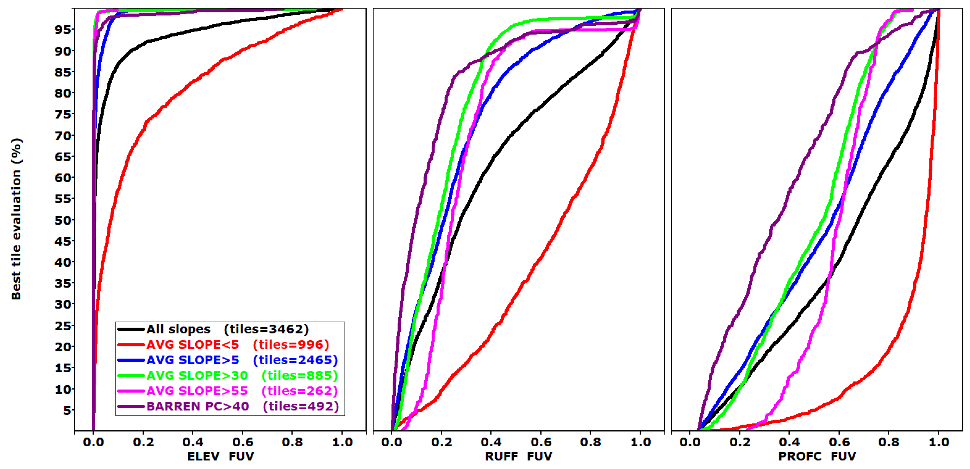
Figure 6 shows summary diagrams of how slope affects the FUV results for three criteria, selected from Figure 4. The degree to which the geomorphometric grids correspond with those computed from the reference DTMs varies with the characteristics of the tile; low FUV indicates the best correspondence comes with larger slopes. Figure 2 shows the FUV criteria with more, finer filters compared with Figure 6. The finer resolution in Figure 2 shows that as the tiles become steeper or rougher, the average evaluations decrease until they reach minima at about 30% average slope and a 10% average roughness. The overall results more closely resemble the reference DTM, although the individual criteria still vary in their effectiveness in Figure 6, whose panels isolate the differences among the selected criteria.

The worst comparisons with the reference DTM occur with average slope under 5% or average roughness under 2%. The results do not show a clear pattern for the effects of forest cover (Figure 2).

The results of the analysis, considering all 17 FUV criteria, indicate the following:

• CopDEM performs the best of the DEMs, with two caveats depending on slope (Figure 7). For slopes above 55%, ALOS performs almost as well, while for slopes below 5%, FABDEM performs better.
• In flat coastal areas, the vegetation and buildings, which still have an effect on CopDEM, have an undue influence on many of the parameters.
• In very flat terrain, SRTM and NASADEM slightly outperform CopDEM for elevation, but not for any of the other criteria.
• For average tile slope under 10%, FABDEM has the best average rank over the 17 FUV criteria.
• Between 10% and 60% slopes, CopDEM ranks best.
• Above a 60% slope, ALOS performs best, but below that point ALOS performs significantly worse than both FABDEM and CopDEM.

CopDEM is always close to the best ranking, and we suggest it be the default compromise choice for general usage.

The previous results indicate that based on our sample, the only DEMs that warrant being considered instead of CopDEM are ALOS and FABDEM. The graphs in Figure 7 show how these compare for each of the 17 FUV criteria. FABDEM performs better for about half the criteria, but only in low-slope areas. ALOS performs better in about half the criteria, but only in the steepest tiles, a relatively small subset of our sample.

3.3. Pixel Raster Classification Criteria

We are using two raster classifications, geomorphons [49] and the 12-category (IP12) geometric signature of Iwahashi and Pike [50]. For each we compute four metrics of accuracy, with results ranging for 0 to 1, to compare the classifications from the test DEMs to the reference DTM. The accuracy measures are adjusted (subtracted from 1) so that a low average ranking is best; 0 would be complete agreement and 1 no agreement. 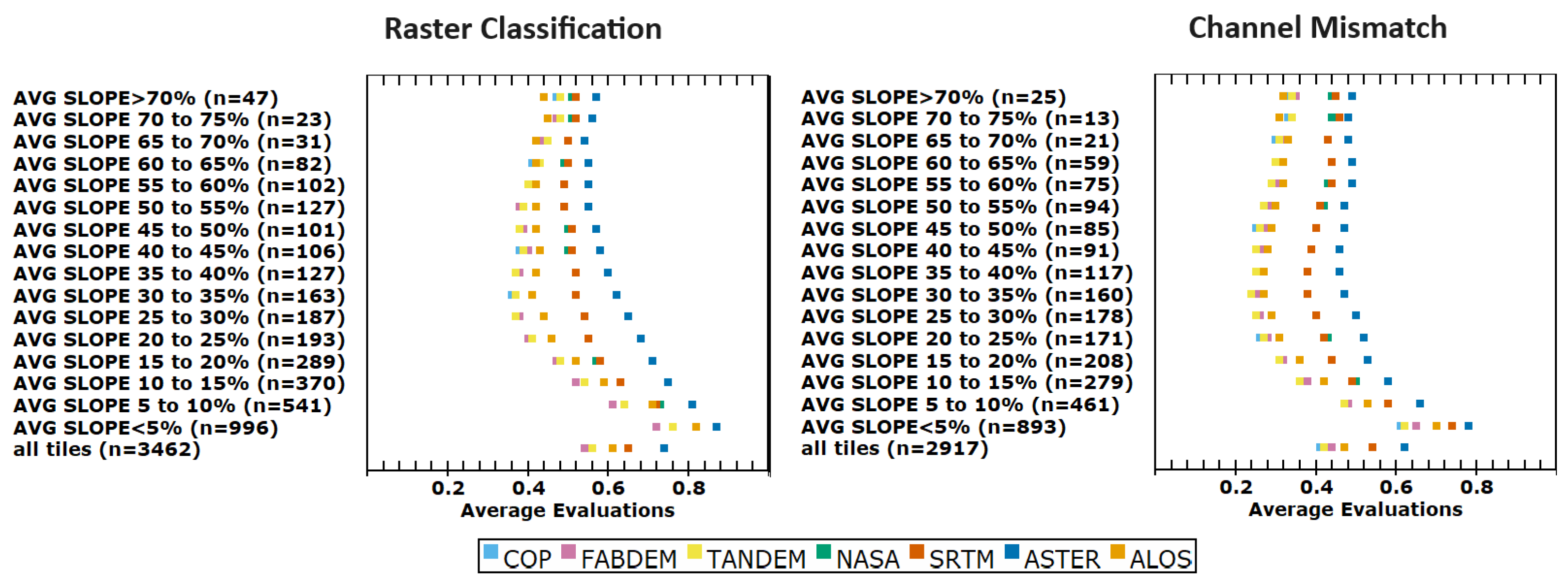Figure 8 shows the average evaluations, with FABDEM and CopDEM ranked best and TanDEM-X very close. The geomorphons perform marginally better than IP12 (Figure S1). Figure S2 shows the distribution of overall accuracy for the best-performing test DEM across the entire data set. The effect of slope mirrors that for the other criteria groupings: best for steeper and barren tiles, and worst for the low-slope tiles. There is a lot of scatter in the evaluation with slope (Figure S3). There are points for 3234 tiles on each panel, so the patterns can be deceiving. Note, however, that the three test DEMs on panels to the right are all on the right half of the cloud of points, meaning they match the reference DTM much more poorly than the others.

Figure S3 shows the performance of the six test DEMs compared to CopDEM. All eight metrics perform in a similar fashion. FABDEM is marginally better than CopDEM, especially in low-slope areas. ALOS outperforms CopDEM in very steep areas, which is the only area where TanDEM-X also outperforms CopDEM for a few metrics.

3.4. Vector Mismatch Criteria

The extraction of drainage networks represents a common use for DEMs, and the results for a single test area (Madrid, Spain) were used as verification of the utility of the DEMIX wine contest’s results [17]. Software can compute drainage networks as a grid or vector files, but each can be converted to the other form; we used grid. We use two metrics: comparing how often the channels derived from the test DEM match the results from the reference DTM, and how often they match exactly or are within a single pixel of the correct location. Figure 8 shows the average evaluations. CopDEM has the best evaluation, but TanDEM-X comes a close second. FABDEM is a step behind and ALOS generally another step back.

Supplementary graphics, which generally duplicate the results for the difference distributions or the FUV criteria: best evaluation by slope category (Figure S4), scatter plots of the tiles by slope and evaluation (Figure S5), and head-to-head comparisons to CopDEM (Figure S6).

3.5. Clustering to Evaluate Geomorphometric Controls on Results

We used K-means clustering to look at the geomorphometric controls on the FUV results and the reliability of the grids underlying the FUV criteria. Clustering allows us to group the data by quality using all 17 FUV criteria, and although the results resemble standard quantiles, the groupings do not all have to have the same number of tiles. Before clustering, we transposed the database so that each row contains a single tile for a single test DEM, and the numerical evaluations for all of the criteria are in separate columns. The number of lines in the database is the number of DEMIX tiles times the number of test DEMs. We requested up to 15 clusters; the K-means algorithm implementation in MICRODEM returned 9. They are numbered from 1 to 9 in terms of increased FUV across the criteria. Cluster 1 best matches the reference DTM, and cluster 9 has the poorest matches.

To visualize the data, we ordered the criteria by increasing value of FUV in the best clusters (Figure 9). The criteria at the bottom of the plot have the test DEMs most closely matching the reference DTMs, and the criteria at the top have the poorest correlations. The lines connect the average evaluation for the criterion labeled on the left for all the DEMs assigned to the cluster. Looking at plots of each tile within a cluster shows substantial scatter, with some overlap between clusters, but the K-means algorithm selected breaks with clear differences in the FUV results between the DEMs in each cluster.

Figure 9 shows how the FUV of the various derived grids varies among clusters, and Figure 10 shows the characteristics of the tiles within each cluster. Combining the cluster information in the two figures, we grouped the nine clusters into three groups, A (clusters 1–3), B (clusters 4–6), and C (clusters 7–9), to graph the locations and test DEMs that best match the reference DTMs.

Some key observations can be drawn from this analysis:

• Except for cluster 9, elevation FUV is generally very low, indicating that the test DEMs compare closely to the reference DTM. Even for cluster 9, the elevation FUV is much lower than any of the other criteria.
• The parameters that require computation of multiple derived grids (LS, WETIN, and HAND) have higher values of FUV, meaning they compare poorly with the reference DTM. Each derived grid needed to compute the grid for a parameter increases the uncertainty in the final grid.
• The second-derivative parameters (e.g., curvatures) behave much worse than most of the others. TANGC and PROFC are better than PLANC and ROTOR.

Maps (Figure 11) show the locations for four of the test DEMs by cluster group, our metric for DEM quality-matching the reference DTM. The largest number of tiles in group A are in the southwestern corner of the United States and Spain. Average tile characteristics for the seven parameters we track show that cluster group A, where the DEM best compares with the reference DEM, is non-urban, low forest, high barren, moderately high elevation, average slope and relief. This is the least forested and least urban cluster.

The test DEMs are not randomly distributed in the clusters (

Table 6. Number of test DEMIX tiles in each cluster.

Cluster	CopDEM	TanDEM-X	FABDEM	ALOS	NASADEM	SRTM	ASTER
Cluster 1	1	1	0	0	0	0	0
Cluster 2	109	100	78	1	0	0	0
Cluster 3	106	98	106	1	0	0	0
Cluster 4	350	306	280	211	0	0	0
Cluster 5	388	336	432	645	12	8	0
Cluster 6	747	634	826	768	873	830	47
Cluster 7	580	673	646	477	1245	1283	1407
Cluster 8	549	633	635	512	657	665	825
Cluster 9	570	618	397	785	613	614	1121

). No DEMIX tiles have NASADEM, SRTM, or ASTER in cluster group A (the best). Group A effectively contains only CopDEM, TanDEM-X, and FABDEM (only two ALOS tiles out of the 601 tiles in the group; the radar-based elevation data source clearly outperformed the optical ALOS instrument). By this analysis, FABDEM corrected or overcorrected a number of these tiles where it should not have. The best performers are concentrated in just four countries and a small number of test areas (

Table 7. Group A test areas.

Country	Test Areas	DEMIX Tiles
USA	18	164
Switzerland	1	1
Spain	7	68
Haiti	1	1

). One tile in Switzerland (N46UE010A) has CopDEM, TanDEM-X, and FABDEM in the group, and Haiti tile N18PW072B has CopDEM and TanDEM-X. This analysis looks beyond just the elevation values and looks at how the DEM captures the spatial patterns about each pixel for 17 different grids.

Cluster group C tiles, the worst performers, are relatively urban or forested. Average elevation, roughness, average slope, and relief all have very low values along the coast. Cluster group C has a substantial number of all the test DEMs; we interpret these tiles (forested, urban, flat coastal areas) as locations where the spaceborne remote sensors do not perform well. We also oversampled these areas so we could compare the new edited DTMs.

3.6. Edited One-Arc-Second DTMs

To compare the edited DTMs with the global data sets, we mask each to the covered area of the one with the smallest elevation range before computing the statistics. This creates four distinct data sets, each of which has a smaller subset of the test areas and tiles compared to the next highest elevation range data set (Table 5). This reduces the number of test areas and DEMIX tiles available for each comparison. To maximize the number of comparisons for the coastal data sets, we oversample coastal data. For reasons to be discussed later, we also consider a data set without coastal sampling areas, which can be created by filtering the FULL elevation range database to remove the flat, low-elevation coastal tiles. Many of the figures (Figure 3, Figure 4, Figure 6 and Figure 7) in the previous sections of the paper show this subset of the data, with an average slope over 5%.

For this evaluation we elected to use the FUV criteria. We hypothesize that the FUV criteria represent a much fuller sample of the potential uses of the DEMs, rather than the difference distribution, which has 15 criteria that are probably redundant, whereas a single criterion for elevation, slope, and roughness would probably being sufficient. The FUV criteria are probably a better representation compared to the raster classification and vector drainage networks, which are based on some of the derived grids in the FUV criteria, and all criteria groups provide very similar rankings.

Comparison of the behavior of test DEMs to the lidar-derived reference DTMs, with CopDEM as the baseline, for all FUV criteria for the U10, U80, and U120 databases (Figure 12) show many of the same patterns observed for the FULL data set (Figure 3, Figures S3 and S6). Each column in Figure 12 adds one additional DEM, but has fewer test tiles meeting the lower elevation limits. The criteria are arranged from top to bottom in the order in which they have increasing FUV; in general, the edited DEMs perform better for the easier criteria (Figure 4) and CopDEM performs better for the difficult criteria. All tiles used in each comparison are also included in the columns to the left, but in most cases the tiles contain fewer comparison points because parts of the tiles are outside the elevation range. The comparison with CopDEM can change between columns because both the number of tiles changes and the compared area in each tile also changes.

Results from the edited DTMs show that as the DTM extends to smaller maximum elevations, the best FUV values decrease (Figure 13; compare with Figure 6). As the panels go from left to right for lower elevation ranges, the curves move farther and farther to the right. This is most clearly shown in the increased distance between the curve for elevation FUV and the others, and the increasing number of criteria close to the right-hand edge of the plots. For low elevations the one-arc-second DEMs do not perform as well as at higher elevations; the low slopes along the coast drive this effect. Many of the low-elevation tiles are also forested and urbanized, increasing the challenges in creating the DEM.

Figure 14 shows the FUV evaluations for elevation, with all tiles in the elevation range graphed. The tiles are sorted by the best evaluation for the tile and the percentile where performance begins to degrade. The colored points depict one DEM in each panel, and the gray values show the other DEMs. The best results are to the left and the best DEM is on the left of the cloud. For U120, U80, and U10, CoastalDEM performs best for elevation.

Figure 15 shows the average evaluation of the FUV criteria by slope category for the different elevation data sets. The patterns for the U120 data set are similar to the full data set, but generally with large FUV evaluations, and the best results at moderate slopes. The U80, and especially the U10 results, show the challenges for all of these DEMs in very flat coastal areas.

The overall average rankings with all the criteria (Figure 12) do not support the superiority of CoastalDEM. The head-to-head comparisons of each of the other test DEMs with CopDEM (Figure 12) show that the edited DTMs can have better elevation, but the training does not necessarily improve the derived grids. The FUV for the derived grids is generally worse than for the starting CopDEM used for the DTM.

3.7. Hallucinations

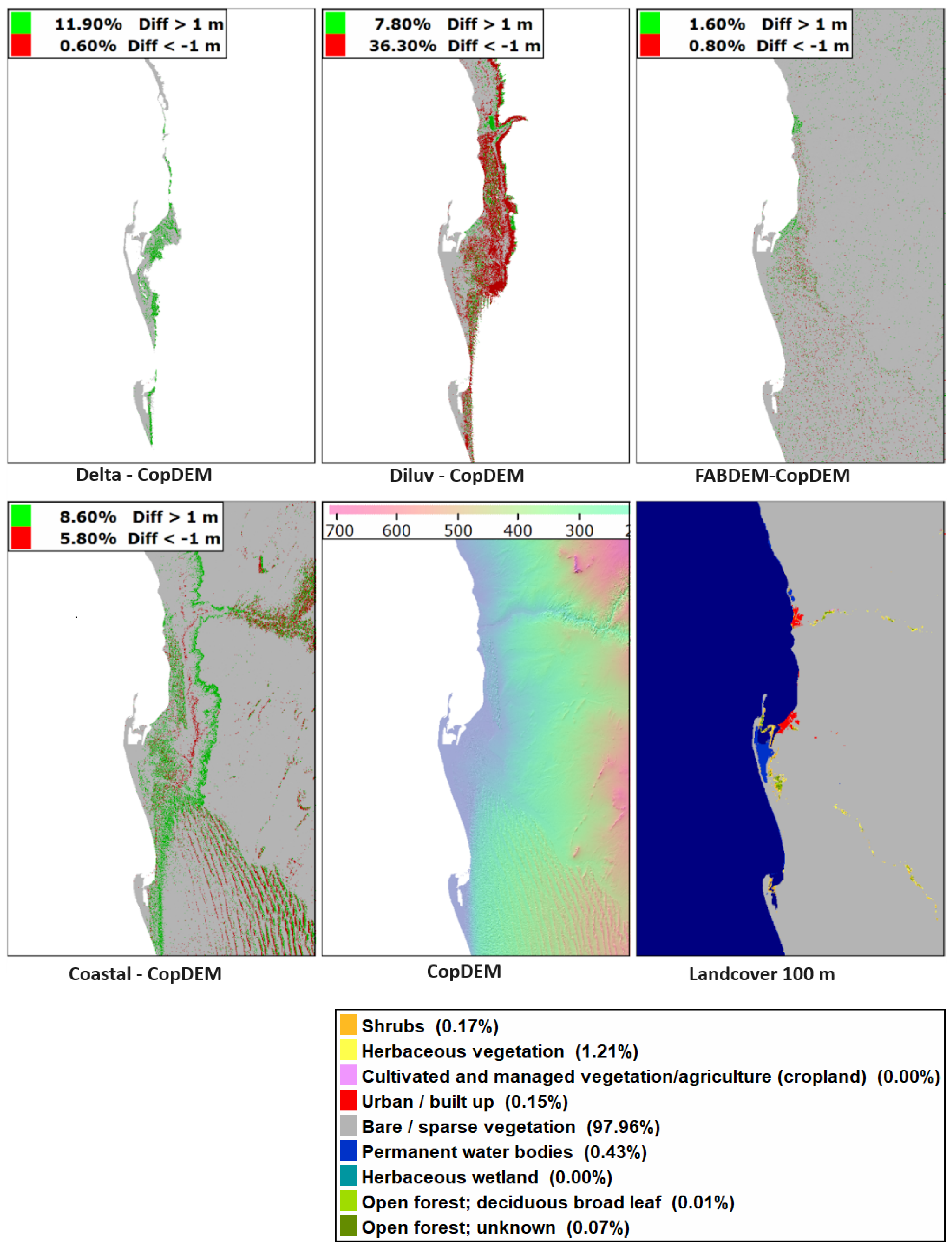
Hallucinations, where artificial intelligence or machine learning algorithms create false answers, occur with some regularity. We use the term to refer to cases when the edited DTM introduces changes to the source DEM that make the new DEM worse than the original DEM. The last section detailed that the edited DTMs generally do not improve derived grids like slope. To look at the extent of hallucinations, we picked a coastal area with very limited vegetation and urban area.

The only global locations with large occurrences of barren coastal areas occur in the Southern Hemisphere on the west coasts of Africa and South America, where we do not have lidar-derived reference data. Figure 16 shows the difference between each of the edited DTMs and CopDEM, from which they are derived, with the 1 m and greater differences highlighted. For some applications 1 m elevation differences might not be severe, but these DEMs are designed for critical use along the shoreline. In this area, minimal changes should have been made to CopDEM, but only FABDEM limited its hallucinations. For CoastalDEM, the large north–south belt of 1 m and greater differences with CopDEM occur at 120 m elevation, the nominal limit for the data set. This indicates problems with the merge between the edits below 120 m and the higher elevations included to fill the one-degree tile.

4. Discussion

Our results assume that the lidar-derived DTMs represent the best available reference DTM. At this point we cannot evaluate this assumption, but we think the airborne lidar will be better than alternatives like ICESat-2 or GEDI, that have been used for many evaluations of the global DEMs, which are point measures with a relatively large footprint. The much higher density of the airborne lidar allows creation of DTMs and the derived grids for our FUV criteria, which is not possible with the linear ICESat-2 or GEDI tracks. With reference DTMs from a wide selection of national mapping agencies, the factors that will affect their matching the actual ground surface include: the age and quality of the source lidar; the filter used to find ground points with potential smoothing; the policy on building and bridge removal and fill, which are much harder than vegetation to deal with; the water filtering or fill of lidar voids; and any hyro-enforcing performed.

4.1. DEM Comparison Methodology

Most previous comparisons of global DEMs have solely looked at difference in elevation to a limited number of reference points, and used a relatively small test region [16]. The DEMIX group extended the analysis to slope and roughness parameters [17]; we extend the number substantially, using 17 different land surface parameters, derived channel networks, and two different terrain classifications. We find the DEMIX group’s 15 criteria redundant because the 5 criteria for each parameter are highly correlated, and they really only compared elevation, slope, and a single roughness index. This was still a big improvement over only looking at a few elevation differences. Differences among the five criteria for each of their parameters represent different behavior on the extreme tail of the distribution, which is not common in these DEMs. Although this might be useful for detailed evaluation of particular areas, we find multiple independent measures to be a better metric to choose the best DEM.

The selection of metrics with a common scale of 0 (best) to 1 (worst), such as those we introduced here for the comparisons, greatly facilitates the analysis compared to the difference distribution criteria for which we could not find an effective way to normalize to a common scale for different areas or criteria. The conclusions that follow would have been much harder to identify had we stayed with criteria like the difference distributions.

The wine contest, with Friedman statistics in a randomized complete block design (RCBD) [17], was designed to allow qualitative criteria in addition to quantitative criteria [17]. The attempt to use the hillshade map and expert judges to rank DEMs [56] showed how hard that would be to run at scale to perform a ranking like this. The quantitative criteria, and results such as Figure 2, highlight that the evaluations themselves have more information value than the statistical rankings.

4.2. Spatial Patterns of One-Arc-Second Global DEM Quality

Challenges in low-relief coastal areas have been extensively documented [57,58]. These issues, and the importance of these highly populated areas, led to the efforts to produce edited DTMs. Our results indicate that in coastal areas one-arc-second DEMs, particularly those derived from the current freely available satellite sensors, may not be the best choice. Much higher-resolution lidar data than 1-arc-second (30 m) may be required to accurately model flooding and sea level rise [59]; our work confirms this.

At the other extreme, mountainous areas also limit the ability for DEMs to capture terrain [54,60,61]. Because of the steep slopes and high roughness in mountainous regions, the combination of horizontal pixel location uncertainty and vertical elevation uncertainty lead to large potential for errors (or just differences) between different DEMs.

Our grouping of the clusters has the best group A, effectively containing only CopDEM, TanDEM-X, and FABDEM (there are two ALOS tiles out of the 601 tiles in the group). The maps of the DEMIX tiles plotted by cluster group (Figure 11) show that the best performers are concentrated in just four countries and a small number of test areas (Table 7). One tile in Switzerland (N46UE010A) has CopDEM, TanDEM-X, and FABDEM in the group, and Haiti tile N18PW072B has CopDEM and TanDEM-X in group A. The remainder of the tiles are in the southwestern United States or Spain.

Figure 10 shows the characteristics of the tiles by cluster.

Table 8. Koppen classification of the group A tiles.

Koppen	DEMIX Tiles	Name
As	2	Tropical savanna—dry summer
BSk	107	Mid-latitude cold steppe
BWh	87	Low-latitude hot desert
BWk	55	Mid-latitude cold desert
Cfa	2	Humid subtropical no dry season hot summer
Cfb	43	Marine west coast no dry season warm to cool summer
Csa	146	Mediterranean summer dry and hot
Csb	67	Mediterranean summer dry and warm
Dfa	3	Humid continental hot summer
Dfb	43	Humid continental mild summer
Dfc	6	Subarctic 1–4 mild months
Dsb	37	Subarctic summer dry mild summer
ET	3	Tundra

shows the Koppen classification [62,63] for the group A tiles. The Haiti tile has a tropical savanna climate, and Switzerland has a tundra climate in this version of the Koppen system. The tiles in Spain and the United States are mostly cold steppe, desert, or Mediterranean climates. The Koppen system uses temperature and rainfall, and the relationship with vegetation was inherent in its creation. These characteristics also expose the ground surface to satellite sensors, which do not have to penetrate significant vegetation. This use of climate might actually reflect vegetation more directly, but we have not found a global vegetation or land cover data set whose categories match the response to the satellite sensors measuring topography.

While we acknowledge the importance of multiple factors in determining the quality of the global DEMs, slope appears to have the most predictable effect. Roughness has a smaller effect, and is not simply correlated with slope. Our data show that for any average tile slope a range of average roughness occurs. Average forest cover and percent barren landscape show much greater scatter in their relationship with FUV.

4.3. Evaluating Reference DTMs

We assume that our reference DTMs are the best available choice to evaluate the test DEMs. Anomalies in the database indicate that in a few cases the reference DTM may account for the low FUV evaluations. Plots of the FUV evaluations versus tile slope highlight anomalies. Figure 17 shows the three representative criteria previously shown (elevation the best, roughness average performer, and profile curvature near the bottom).

For roughness, 21 tiles have moderate slope on the far right, where all the test DEMs have FUV almost 1. They are all in Italy (Tiburon,5 tiles, and Bolzano,16 tiles), and because all the test DEMs have such similar evaluations we suspect the reference DTM.

For elevation, five tiles with moderate slope and elevation FUV are in the middle of the plot, far away from the main trend of the test data. These are in Tiburon (four tiles) and Norway (one tile), and all of the test DEMs have nearly identical FUV scores, again indicating potential problems with the reference DTM.

The Haiti data set likely presented a challenge to collect in 2010 [64], so it is not unexpected that it has problematic tiles, although it also is one of the few test areas to have one of the group A (best) tiles discussed in the last section. Bolzano has a large fraction of its test tiles in the lowest clusters, more than the other areas in Italy with roughly similar Alpine terrain. It was beyond the scope of this paper to investigate individual tiles, but the global DEMs might be a quality control measure for lidar studies when all the global DEMs fail to match a DTM aggregated to their scale.

4.4. Gaps and Data Fill in Global Arc-Second DEMs

None of the global DEMs managed to map every pixel on land, and after the initial releases of SRTM with voids, a number of void filling algorithms appeared. Later editions of all the DEMs used various other available DEMs to fill the voids. Metadata files, commonly ignored, show which pixels were filled and with what other DEM. Summaries by DEMIX tile show the primary data fraction (PDF), the percentage of the tile using original data from the sensor [65]. The fact that a pixel was filled indicates the sensor could not resolve the elevation, but different producers might set different thresholds for when they choose to use fill from another DEM. The producer tolerance might change over time, and if they correctly replace a pixel with a better elevation, the quality of the DEM increases.

Our database [24] contains the PDF for each DEMIX tile extracted from [65]. Figure 10 shows, in the bottom right two panels, the PDFs for CopDEM and ALOS for the nine clusters we extracted to rank DEM performance. CopDEM used more fill pixels than ALOS, with clusters 1 and 2, the best performers, having the fewest voids. In the higher slope and barrenness categories, CopDEM has substantially more filled voids compared to ALOS, indicating the choice of fill was not optimal, and in these tiles ALOS outperforms CopDEM. A full discussion of the reasons for this is beyond the scope of this paper, as it would require looking at the metadata grids with the fill information for all 3424 tiles. This highlights the importance for users to understand the metadata available with these DEMs. Future editions of CopDEM would benefit from improving the DEMs used for fill.

4.5. Parameter Ranking Based on FUV Performance

The FUV parameters can be ranked in terms of how well they perform for the test DEMs relative to the reference DTM. Figure 4 sorts the criteria in terms of the average FUV in cluster group A, which had the highest correlation.

Table 9. Ranking of FUV criteria based on parameter robustness.

Field	Meaning	Mean FUV	${\mathit{r}}^2$
ELEV FUV	Elevation	0.0001	0.9999
HILL FUV	Hillshade	0.0093	0.9907
SLOPE FUV	Slope	0.0202	0.9798
OPEND FUV	Downward openness	0.0279	0.9721
TPI FUV	Terrain position index	0.0279	0.9721
OPENU FUV	Upward openness	0.0285	0.9715
RUFF FUV	Roughness	0.0358	0.9642
CONIN FUV	Convergence index	0.0367	0.9633
HAND FUV	Height above nearest drainage	0.0789	0.9211
RRI FUV	Radial roughness index	0.0832	0.9168
TANGC FUV	Tangential curvature	0.0875	0.9125
PROFC FUV	Profile curvature	0.1169	0.8831
WETIN FUV	Wetness index	0.1271	0.8729
LS FUV	LS factor	0.2096	0.7904
ROTOR FUV	Rotor	0.2867	0.7133
ACCUM FUV	Flow accumulation	0.5040	0.4960
PLANC FUV	Plan curvature	0.5129	0.4871

orders the criteria, listing the FUV and corresponding squared Pearson correlation coefficient. Elevation has by far the best evaluations with low FUV, but several other criteria perform well. As a group the curvature measures perform poorly, especially plan curvature. Unexpectedly, flow accumulation, critical for many hydrological studies, has almost the highest FUV in Table 9.

This ranking applies strictly only to the first cluster, which we interpret as being most amenable to creating a one-arc-second DEM from space. It is almost entirely based on the radar sensor used in CopDEM and TanDEM-X, but applies broadly to all the test tiles. Cluster 2 has slightly higher FUV values for all of the criteria, with a large spike (indicating poorer overall performance) in plan curvature. Cluster 3 follows cluster 2, but the convergence index and tangential curvature both spike. The tile characteristics in the clusters (Figure 10) show that the percent of the tile that is forested increases substantially. Cluster 1 includes tiles with very high percentage forested values derived from land cover [31] for arid forest areas in the Canary Islands and desert southwest of the United States, where the low vegetation density classified as forest apparently does little to affect the radar sensor used for CopDEM. The real drop in performance occurs with cluster 4, with a noticeable spike in tangential curvature and large increases for all parameters other than elevation.

Many users assume that global DEMs can function as a DTM. Depending on the particular DEM, the characteristics of the area, and the parameter involved, the degree of error introduced will vary. Table 9 allows users to assess the effect of using a DSM and assuming it is a DTM. For criteria at the top of the table, the global DEMs closely match a reference DTM. Moving down the table, the DSMs increasingly fail to match the reference DTM. The overall results for CopDEM show that it performs better at penetrating the vegetation canopy compared to any of the other global DEMs. A DTM also requires removing buildings, which none of the global DEMs can, but vegetation is far more prevalent in our data sample compared to buildings (Figure 10 shows the small percentage of urban area in almost all of our test tiles). Our tile sampling could affect this result for forests, because we could not obtain tiles with quality reference DTM data in dense tropical forest. We append an FUV to the criteria names because we envision using additional metrics to measure the similarity between the test and reference grids.

5. Conclusions: Which Global DEM to Use?

Figure 7 and Figure 12 summarize our results for the best of the one-arc-second DEMs. For full consideration of the DEMs not included, use the database [24]. Overall, CopDEM does the best job preserving the most derived parameters while performing well compared to a DTM, even though CopDEM is closer to a DSM, penetrating vegetation somewhat. In very rough terrain ALOS may perform better for many metrics. Of the edited DTMs, CoastalDEM performs best for elevation in all three elevation ranges, U120, U80, and U10, but for many other criteria FABDEM performs better. The performance of all these DEMs in the U10 category is limited and an airborne lidar solution would be much better. The U10 elevation range directly along the shoreline will be critical to address global climate change.

Based on its lack of a restrictive license and overall performance across all of our criteria, CopDEM would be appropriate as the default global one-arc-second DEM. CopDEM already uses national lidar in Norway, and future editions would benefit from adding coastal lidar where available for those critical areas to further improve the product.