Article

Statistically Resolved Planetary Boundary Layer Height Diurnal Variability Using Spaceborne Lidar Data

by
Natalia Roldán-Henao
1,
John E. Yorks
2,*,
Tianning Su
3,
Patrick A. Selmer
2 and
Zhanqing Li
1
1
Department of Atmospheric and Oceanic Sciences and ESSIC, University of Maryland, College Park, MD 20740, USA
2
NASA Goddard Space Flight Center, Greenbelt, MD 20771, USA
3
Lawrence Livermore National Lab, Livermore, CA 94550, USA
*
Author to whom correspondence should be addressed.
Remote Sens. 2024, 16(17), 3252; https://doi.org/10.3390/rs16173252
Submission received: 30 July 2024 / Revised: 26 August 2024 / Accepted: 27 August 2024 / Published: 2 September 2024
(This article belongs to the Special Issue Observation of Atmospheric Boundary-Layer Based on Remote Sensing)

Abstract

:
The Planetary Boundary Layer Height (PBLH) significantly impacts weather, climate, and air quality. Understanding the global diurnal variation of the PBLH is particularly challenging due to the necessity of extensive observations and suitable retrieval algorithms that can adapt to diverse thermodynamic and dynamic conditions. This study utilized data from the Cloud-Aerosol Transport System (CATS) to analyze the diurnal variation of PBLH in both continental and marine regions. By leveraging CATS data and a modified version of the Different Thermo-Dynamics Stability (DTDS) algorithm, along with machine learning denoising, the study determined the diurnal variation of the PBLH in continental mid-latitude and marine regions. The CATS DTDS-PBLH closely matches ground-based lidar and radiosonde measurements at the continental sites, with correlation coefficients above 0.6 and well-aligned diurnal variability, although slightly overestimated at nighttime. In contrast, PBLH at the marine site was consistently overestimated due to the viewing geometry of CATS and complex cloud structures. The study emphasizes the importance of integrating meteorological data with lidar signals for accurate and robust PBLH estimations, which are essential for effective boundary layer assessment from satellite observations.

1. Introduction

The planetary boundary layer (PBL) is the layer of the atmosphere nearest to the Earth’s surface, which is characterized by intense turbulence [1,2]. This turbulence is influenced by various surface forces, such as frictional drag, heat, and momentum fluxes, which ultimately affect the intensity and height of the PBL [3,4,5,6] can vary significantly depending on time and location, ranging from just a few tens of meters during stable conditions (usually at night or early morning) to over a kilometer during unstable or convective regimes (usually in the afternoon). The PBL fundamentally mediates the interactions between the Earth’s surface and the atmosphere and ultimately helps to connect the atmosphere to other Earth system components, bridging the gap between weather and climate [7,8,9].
Accurately estimating the planetary boundary layer height (PBLH) is crucial for various earth science applications, such as climate modeling, numerical weather forecasting, and air quality analysis [10,11,12,13]. Observational estimates of the PBLH include the use of radiosondes [14,15], radars [16], spaceborne and ground-based backscatter lidars [17], ceilometers [18], aircraft [19], Radio Occultation technique [20], and more. These observations have significantly improved our knowledge of boundary layer meteorology and climate, leading to the development of more advanced parameterizations that are critical for modeling endeavors [13]. Nevertheless, despite recent advancements in observations and estimation techniques, the diurnal variations of PBLH on a global scale remain inadequately understood. This gap in understanding is partly due to the limitations of current observation techniques. For instance, radiosonde measurements are temporally constrained, and lidar-based measurements lack comprehensive spatial coverage.
Obtaining global distributions of the PBLH is feasible through satellite observations. In previous studies utilizing spaceborne lidars, the PBLH was computed using the Cloud-Aerosol Lidar and Infrared Pathfinder Satellite Observation (CALIPSO), a sun-synchronous satellite that passes over the equator at 1:30 am/pm [21]. CALIPSO is capable of providing high-resolution vertical distributions of clouds and aerosols, making it a valuable tool for estimating global PBLH from space [22,23,24,25]. Various methods have been employed to compute PBLH from CALIPSO data, such as the lowest occurrence of a local maximum in the vertical standard deviation of the lidar backscatter profile, as used in [22,26]. Other methods include traditional lidar-based algorithms, such as the gradient method and the wavelet covariance transform function [17] but tend to only capture the top of the residual layer during nighttime conditions.
While utilizing CALIPSO offers a daytime-nighttime contrast of the PBLH, it has a limitation in observing the full diurnal variability of the boundary layer due to its fixed overpass times. On the other hand, the Cloud-Aerosol Transport System (CATS) on the International Space Station (ISS) provides vertical backscatter profiles at variable overpass times, allowing for the global statistical resolution of the PBLH’s diurnal cycle [27]. Previous studies have investigated the spatiotemporal variability of the PBLH using CATS data. Palm et al. [28] utilized a threshold approach and a convolutional neural network to estimate the PBLH, exhibiting the ability of CATS data to retrieve the PBLH on seasonal and global scales, but not diurnal scales. Recently, Li et al. [29] statistically resolved the diurnal cycle of the PBLH using CATS data on a near-global scale, showing a 0.6 correlation with radiosonde estimates for clear sky conditions during the daytime only and demonstrating CATS’ potential to retrieve the diurnal variation of the PBLH. However, the authors averaged CATS daytime files to 60 km and excluded instances with cloud bases below 5 km before computing the PBLH, omitting relevant information provided by cloud-topped boundary layers.
To improve the PBLH retrievals from CATS, this research applies a modified version of the Different Thermo-Dynamics Stabilities (DTDS) algorithm [30] to retrieve the PBLH. Previously, DTDS has been successfully used with ground-based lidar sensors [31], offering improved vertical consistency and temporal continuity, especially during stable conditions compared to gradient or wavelet covariance methods. By applying the DTDS algorithm to spaceborne lidar data from CATS, this study allows for direct comparison between satellite and ground-based lidar measurements using the same method, enhancing the robustness of the analysis. The study leverages data from the Atmospheric Radiation Measurement (ARM) program, a leading climate research facility that offers long-term field measurements and comprehensive atmospheric datasets, to validate the PBLH estimates. Using both denoised daytime and regular nighttime CATS data, the research ensures consistent PBLH detection across all hours of the day. This refined approach aims to improve the capability of obtaining PBLH diurnal variability from satellite observations.
The paper is structured as follows: Section 2 provides an overview of the data and geographical locations used in this study. Section 3 describes the modifications made to the original DTDS algorithm and summarizes the denoising technique applied to the daytime files. Section 4 presents the results for a continental and a marine site, highlighting the advances and limitations of the current study and the methodology used here. Lastly, Section 5 provides a final summary.

2. Data and Geographical Information

2.1. The Cloud-Aerosol Transport System (CATS) Data

CATS was an elastic backscatter lidar that operated on the International Space Station (ISS) from February 2015 to October 2017. Because the ISS has a precessing orbit with a 51.8° inclination angle, CATS was able to sample the atmosphere with a unique frequency compared to other NASA A-Train sensors like CALIPSO or MODIS [32]. CATS collected data with a repeat cycle of nearly 3 days (2.3 days in the midlatitudes and 4.3 days in the tropics), passing over the same locations but at different local times [27]. This enabled CATS to sample the entire diurnal cycle approximately every 60 days, making it an ideal sensor for studying the diurnal evolution of clouds, aerosols, and the PBLH between 51°S and 51°N [28,32,33,34].
CATS provided ranged resolved vertical backscatter profiles and depolarization ratio primarily at 1064 nm, information that is used to retrieve the properties of cloud and aerosol layers on a global scale through their Level 1B and Level 2 products. The Level 1B product primarily consisted of attenuated backscatter coefficients, depolarization ratios, and meteorological data obtained from NASA’s Global Modeling and Assimilation Office (GMAO) [27,35]. These data were provided at a horizontal resolution of 350 m (along-track) and a vertical resolution of 60 m. The Level 2 operational (L20) data consisted of a layer detection and cloud-aerosol discrimination product that included variables such as the layer top and base, feature type, cloud phase, and aerosol type [36].
This study used both CATS Level 1B product version 3 and the Level 2 Operational (L2O) product. For the Level 1B product, we used the total attenuated backscatter, and meteorological variables (temperature, atmospheric pressure, and relative humidity profiles) provided in the CATS data products obtained from the MERRA-2 reanalysis data. For the L2O product, we utilized the cloud top height (CTH), cloud base height (CBH), the DEM Mean Elevation, and feature type.
Several differences between spaceborne lidars like CATS and ground-based lidars impact the methodology and results of this paper. Notably, spaceborne lidars operate from satellite platforms located at much greater distances from the Earth’s surface, often spanning several hundred kilometers or more. These long distances lead to a lowered signal-to-noise ratio (SNR) in spaceborne lidars compared to their ground-based counterparts. The weakened return signals result primarily from longer travel distances, which can be much lower than the solar background noise. Consequently, spaceborne lidars struggle to detect weak or distant targets such as thin clouds or aerosol layers, complicating the determination of a precise PBLH. Conversely, ground-based lidars benefit from closer proximity to surface features, yielding stronger return signals and, thereby, a higher SNR. This enhanced SNR enables ground-based lidars to detect atmospheric and surface features with higher accuracy and precision.
During daytime hours, CATS’s SNR is additionally compromised by the solar background noise. This lowered SNR is reflected in the minimum detectable backscatter (MDB) values of CATS, which vary between nighttime and daytime. MBD serves as a parameter to assess the ability of lidar to measure radiatively important features in the atmosphere; a smaller MBD indicating a better performance. For CATS data at 1064 nm, the MBD is 5.00 × 10⁻⁵ for nighttime and 1.30 × 10⁻³ for daytime hours. In other words, the backscatter signal measured by CATS is noisier during daytime operations compared to nighttime. This noisier signal further complicates the estimation of the PBLH under daytime conditions.
Spaceborne lidars like CATS observe Earth’s atmosphere from a top-down perspective, making them excellent for detecting cloud top height. However, in cases with optically thick clouds, the backscatter signal is strongly attenuated below the cloud top, obscuring cloud base height and boundary layer properties. In contrast, ground-based lidars are ideal for monitoring cloud base height, though the signal is attenuated above the cloud base for optically thick clouds, hiding the cloud top signal. These contrasting yet complementary viewing geometries pose challenges in adapting ground-based algorithms to CATS signals, especially for retrieving the cloudy PBLH. Robust PBLH retrievals, as underlined by Su et al. [37], require knowledge of cloud-surface coupling, typically unknown from spaceborne lidars. The CATS viewing geometry not only affects PBLH retrievals during cloudy conditions but also has implications for nighttime boundary layer retrieval. During nocturnal hours, spaceborne lidars initially detect the aerosol residual layer, where a strong gradient in attenuated backscatter is usually observed, before the backscatter signal becomes strongly attenuated, limiting their ability to detect the top of the stable boundary layer (SBL), which tends to have a very weak (if any) attenuated backscatter gradient compared to the residual layer. Despite their proximity to the SBL, ground-based lidar detection of this layer is challenging due to the weak or non-existent attenuated backscatter gradient.

2.2. The Atmospheric Radiation Measurement (ARM) Data

The U.S. Department of Energy (DOE) ARM program is a scientific initiative that aims to enhance the comprehension and modeling of atmospheric processes, with a particular interest in radiative transfer, clouds, and aerosols. For more than three decades, ARM has gathered extensive data on a large number of atmospheric variables at three permanent sites and various mobile facilities worldwide. This study focuses on two ARM permanent sites, namely the Southern Great Plains (SGP) and the Eastern North Atlantic (ENA). Figure 1 shows the geographical location of both sites in colored dots, and the squared boxes represent an area of 8° × 8° where the CATS backscatter data is taken. For each site, we used the vertical profiles of backscatter radiation measured by a 532 nm micropulse lidar (MPL). Furthermore, we incorporated additional ARM information such as Cloud Boundaries (CBH and CTH) from the CLDTYPE ARM product [38], along with detailed meteorological data, including atmospheric pressure, temperature, and relative humidity [39]. Radiosonde measurements provided further insights into the vertical profile of the atmosphere [40]. These datasets significantly enhance the comprehensiveness and accuracy of our PBLH analysis.
The SGP is the first and most comprehensive observatory of the ARM program, being operational since the 1990s [41]. The SGP site central facility (SGP C1) is located in a rural landscape dominated by cattle pasture and wheat fields, with nearby oil and gas refineries that add complexity to the local environment [42]. As a midlatitude and midcontinental observatory, the SGP provides valuable insights into atmospheric properties influenced by both synoptic and local-scale patterns. Low-level clouds, such as warm boundary layer clouds, are prevalent at this site and exhibit distinct diurnal variations, with nighttime liquid water paths consistently higher than daytime values [43]. The cloud bases at this continental site are usually located below 1 km, exhibiting higher bases during the summer months [44]. In contrast, the ENA site is located on Graciosa Island within the Azores archipelago of Portugal, and a marine environment surrounds its area of 60.7 square km. This site is a stratocumulus to cumulus transition region, characterized by a persistent layer of low-level clouds below 2 km that consists of a mix of stratiform and cumulus cloud regimes [32,45].

3. Methodology

3.1. Denoising Raw Photon Counts

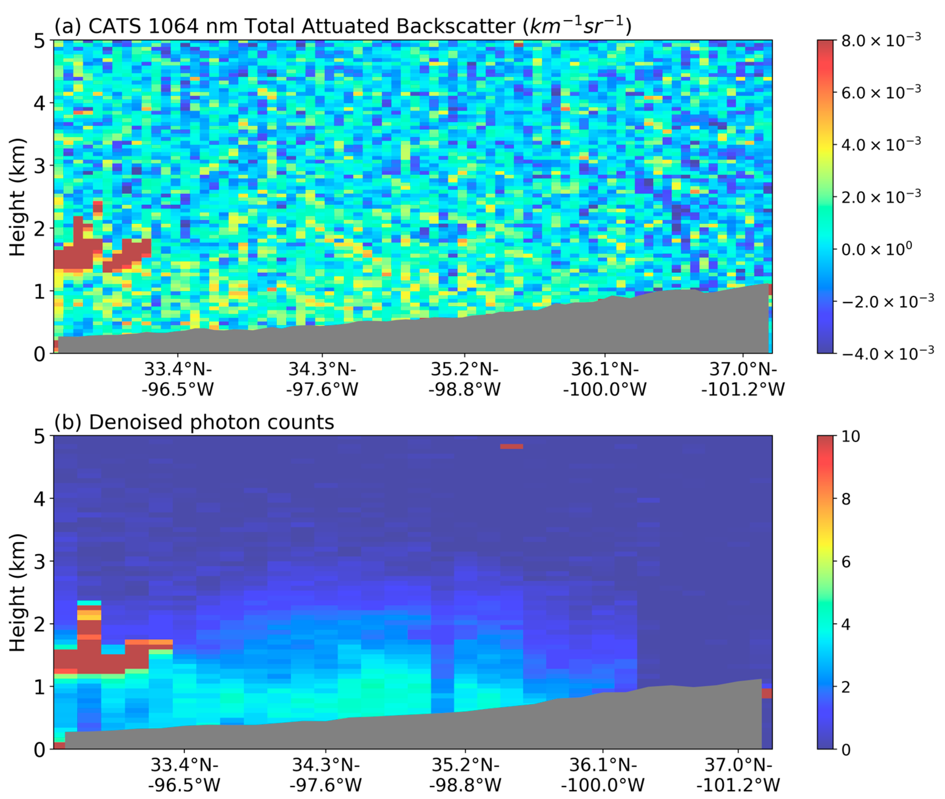
The detection of atmospheric layers and determination of the PBLH is particularly challenging during daytime hours when the high solar background noise significantly obscures the signals of interest. To address this issue and improve the robustness of our analysis, we implemented a deep learning-based denoising approach that improves the SNR of daytime files without coarsening the spatial resolution. Here, we utilized a Deep Neural Network architecture based on a Dense Dense U-Net (DDUNet) model that offers a more complex learning approach incorporating cascading UNets, multi-scale processing, and parameter conservation [46]. Selmer et al. [47] presents a detailed description of the deep neural network architecture and hyperparameters. A training dataset was created using pairs of (1) noisy (daytime simulations created by adding artificial Poisson noise to nighttime CATS data) and (2) noise-free (actual nighttime CATS data) lidar data. The DDUNet model is then trained using these pairs and applied to the CATS daytime data over the SGP and ENA sites to predict residual noise and then subtract the noise from the daytime CATS data. Figure 2 shows an example of the resulting denoised photon counts for daytime CATS data over the SGP site on 11 July 2015. For Figure 2, the denoised photon counts are averaged to 1.8 km along track, while the 1064 nm total attenuated backscatter (Figure 2a) is at the raw horizontal resolution of 350 m. However, we average both to 10 km for input into the DTDS algorithm. Aerosol in the daytime mixed layer is consumed by the solar background noise in the raw CATS daytime data (Figure 2a) but becomes apparent to the eye once the DDUNet denoising method is applied to the data and more similar to the data from the ground-based lidar at the SGP site (Figure 2b). Here, we used daytime denoised photon counts to compute the PBLH.

3.2. Retrieval of the PBLH from Satellite Information Using Traditional Lidar-Based Algorithms

To determine the PBLH from lidar-based information, the underlying assumption is that aerosols are trapped inside the PBL, resulting in a clear contrast between aerosol loading inside the PBL and the surrounding atmosphere. The backscatter signal effectively captures this contrast, mostly during convective boundary layers (CBL), rendering the lidar an ideal tool for PBLH determination. Various methodologies have been proposed for assessing the PBLH from satellite-based lidars, such as CALIOP and CATS, including the maximum standard deviation (MSD), the wavelet covariant transform function (WCT), and the threshold method, all of which are based on this principle.
The MSD method identifies the PBLH by locating a local maximum in the vertical standard deviation of the lidar backscatter [22]. This approach has been successfully applied to both CALIOP and CATS data, demonstrating moderately good performance during daytime hours compared to MPL and radiosondes products [25], particularly in situations with sufficient aerosol loading. The WCT, first introduced by Gamage and Hagelberg in 1993 as a tool for distinguishing step changes from noisy signals, has proven more effective for estimating PBLH using lidar data [48]. The WCT method is defined as follows:
W f a , b = z b z t B z   h z b a d z
where a is the dilation factor, b is the vertical translation factor where the function is centered, B(z) is the backscatter signal, z is altitude, and z b and z t are the integration limits of the Haar function (h). The integration limit, z t , represents the maximum altitude at which the PBLH could grow. For the SGP site, radiosonde observations indicate that the maximum PBLH values are 4.3 km during the day and 2.5 km at night. These values were used as the upper integration limit, z t . At the ENA site, ground-based observations indicate that the PBLH can be as high as 2 km (Figure S2). Given the large heat capacity of the ocean, marine PBLH doesn’t have substantial diurnal variations, so for the entire day at ENA, we use 2 km to capture maximum values. The haar function is defined as:
h z b a = + 1 :           b a 2 z b 1 :           b < z b + a 2 0 :                           e l s e w h e r e
The effectiveness of WCT methods hinges on the careful selection of the dilation factor, typically ranging between 100 m to 1 km. Identifying the ideal value is challenging as it should align with the depth of the entrainment layer, a parameter that is often unknown [29]. Prior research on PBLH computation utilizing CALIPSO data has determined that the best performance is achieved when using a dilation term of 600 to 900 m based on sensitivity analysis [49]. Specificly, this study employs a dilation factor of 400 m, in line with the previous study for the ground-based lidar [30].

3.3. Retrieval of the PBLH from Lidar Data Using DTDS

While traditional methods have been found to provide sound estimations of the PBLH during CBL and neutral boundary layers (NBL), they encounter several issues during SBL, transition periods, cloudy conditions, or during nighttime hours due to the presence of a residual layer. Su et al. [30] addressed some of these limitations by developing the DTDS algorithm. This method uses aerosol backscatter profiles with a stability-dependent model of PBLH temporal variation. DTDS has been shown to perform better under most thermodynamic situations, particularly for SBL and CBL, with higher correlations and smaller errors [31].
The DTDS algorithm is constructed using the traditional WCT and a gradient method, with a selection scheme that determines whether the PBLH is during growing, decaying, or other periods. Unlike traditional methods that use a single backscatter profile to determine the PBLH, DTDS considers current and previous estimations, resulting in a more comprehensive estimation of the PBLH with improved vertical consistency and temporal continuity. First, the local maximum positions (LMPs) in profiles of the wavelet covariance transform function derived from lidar backscatter are identified as potential positions of the PBLH. In the case of CATS denoised daytime files, the LMPs are derived from the denoised photon counts provided by the DDUNet. To ensure good continuity, different stages of PBL development are considered. DTDS-derived PBLHs typically increase during the growth stage and decrease during the decaying stage. However, the algorithm can also identify decreases during the growth stage or increases during the decaying stage based on the available LMPs. When complex aerosol structures (e.g., the residual layer) are present, multiple step signals in the backscatter profiles lead to several PBLH candidates, from which we select the appropriate one based on temporal continuity.
In addition, DTDS can also handle cloudy situations by evaluating the cloud-surface coupling. The methodology classifies clouds as coupled or decoupled to the surface utilizing the lidar-based PBLH estimations, the cloud base height, and the lifted condensation level (LCL). This differentiation aids in accurately diagnosing the PBLH under the cloudy condition [37]. This study applied the DTDS algorithm to estimate the PBLH using both CATS data and ground-based Micropulse Lidar (MPL) observations for both daytime and nighttime periods. Lidar-based techniques face significant challenges in estimating the PBLH during nocturnal boundary layers, particularly below the residual layer. Consequently, most lidar-based algorithms, including DTDS, are typically designed for daytime applications. Given the notably robust SNR of CATS’ nighttime data, we sought to extend the application of DTDS to both daytime and nighttime hours.
Since the original DTDS algorithm was tailored for daytime conditions, we adapted it for nighttime use with ground-based MPL data. This involved running the original DTDS algorithm using both nighttime and daytime backscatter information. Since nighttime turbulence is weak and vertical motion is suppressed within the boundary layer [1], we classify nighttime hours as “other periods” in the DTDS’ selection scheme instead of selecting the growing or decaying periods. Figure S1 in the supplementary information, shows the relationship between the ground-based MPL PBLH and the radiosonde estimates. This study utilizes MPL-derived PBLH estimates and radiosonde data to assess the accuracy of PBLH estimations derived from CATS observations. However, it is important to note that both methodologies are based on different definitions and approaches to evaluate the boundary layer. Lidar PBLH’s retrievals are based on a thermodynamic effect approach, and radiosonde PBLH’s retrievals are based on a substance distribution approach. In the case of the substance distribution approach, the PBLH is retrieved based on the spatial distribution of tracers, such as water vapor or aerosols. Hence, its concept differs from a boundary layer derived from turbulent motions. The difference between the two approaches is more significant when the turbulent transport is weak at nighttime. Still, this substance accumulation layer corresponds to the convective boundary layer during the daytime [50].
Due to the varying measurement methods used by the ground-based MPL and CATS lidar, it is necessary to modify the DTDS algorithm to accommodate satellite data. The original and satellite versions of DTDS differ in several ways, including:
  • The ground-based data allows for continuous tracking of the diurnal variation of the PBLH, enabling the original DTDS algorithm to account for both growing and decaying periods within a single day. In contrast, CATS statistically resolves the diurnal cycle but does not capture those growing or decaying periods in a single pass. Therefore, the adjusted version of DTDS only incorporates “other periods” from the DTDS selection scheme.
  • DTDS algorithm tackles cloudy situations by examining the coupling between the cloud and its surface. Obtaining the PBLH in cloudy conditions is crucial for enhancing the reliability of lidar retrieval systems, as emphasized by Li et al. [29] in their work with CATS. This process necessitates knowledge of the CBH, which can be readily obtained through ground-based lidar. However, the viewing geometry of satellite lidars (such as CATS) renders their signal highly attenuated beneath the cloud top. As a result, the CBH is often impossible to discern for optically thick clouds. To address this challenge, the modified version of the DTDS focuses exclusively on single-layer clouds that are less than 1 km thick and with a CTH lower than the maximum integration limit ( z t ) of the Haar function (see Section 3.2). It is important to note that accurate determination of the cloud thickness depends on knowledge of its CBH. Consequently, we only used CATS data from cloudy conditions in which the mean Feature Type CATS’ classification between the cloud base and the earth’s surface is lower than 3, indicating that the CATS signal is not entirely attenuated beneath the cloud base, and hence, an aerosol layer or ground surface is observable below the cloud base. This serves as confirmation that the estimated CBH is an authentic value and not a byproduct of cloud attenuation.
  • DTDS evaluates the cloud-surface coupling using the LCL. This value is computed based on an exact expression [51] and using ARM’s surface meteorological data (relative humidity, temperature, pressure). Since CATS does not have collocated meteorological measurements, the representation of the LCL is not as robust as ground-based meteorological measurements. CATS meteorological data originates from MERRA-2 reanalysis data at coarse horizontal resolutions (0.5° lat × 0.625° lon), and this data is interpolated down to the CATS horizontal resolution of 5 km; natural variability and interpolation errors can lead to biases in the computed LCL. Therefore, instead of using individual LCL values, our modified version uses the mean LCL value computed from the mean temperature, relative humidity, and atmospheric pressure profiles provided in the CATS data files for the defined ARM-site grid box.
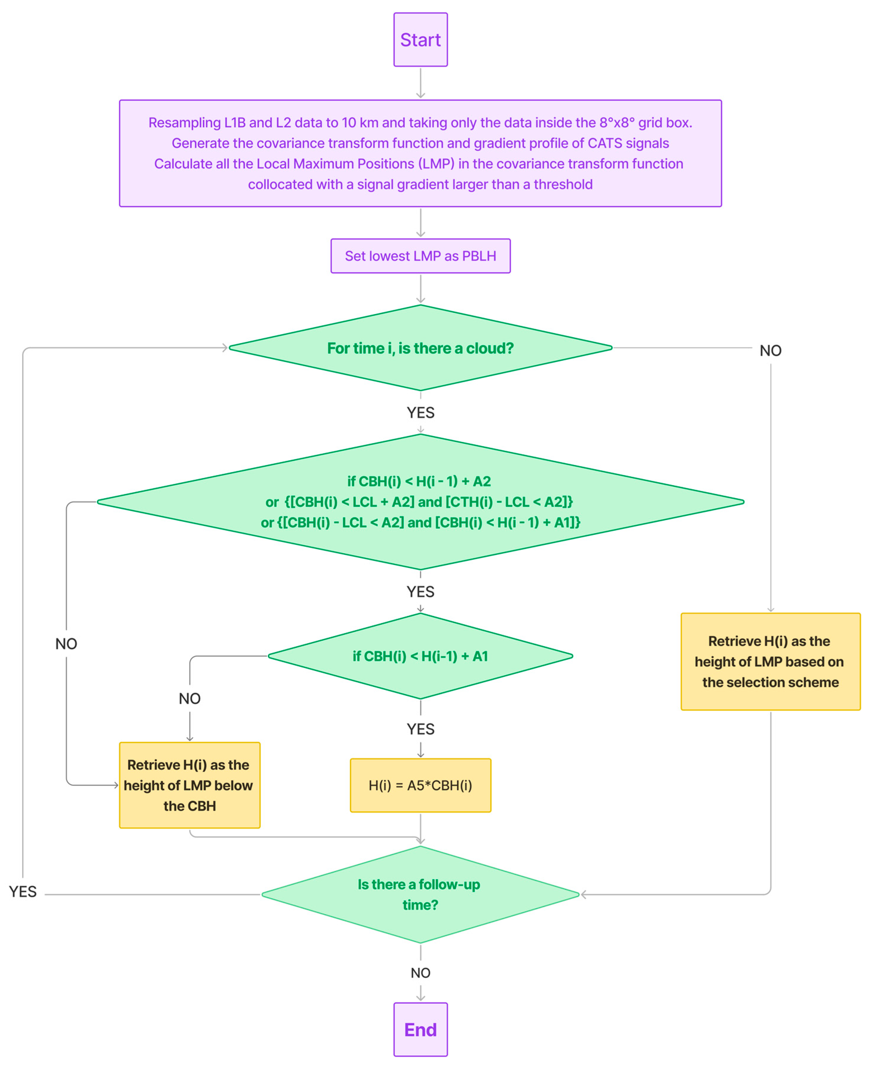
The modified DTDS algorithm adapted for use with CATS is summarized in Figure 3. This diagram includes both determining PBLH under clear sky conditions using the LMPs and handling the PBLH under low cloud conditions. It’s worth noting that the general process of this diagram follows [30,37], although we have removed some LCL constraints from the cloud-surface coupling evaluation. This LCL constraint consists of determining whether or not the computed PBLH was below the LCL value, and if it wasn’t, forcing the PBLH to be placed below it. However, using such constraint led to the PBLH being assigned to or near the LCL altitude frequently, even when the computed LCL was not correlated with the observed aerosol layer due to the LCL errors described above. The experimental parameters A1, A2, and A5 are given by Su et al. [37] as 0.7, 0.2, and 1.1, respectively. As mentioned before, instead of using one single backscatter profile to estimate the PBLH, DTDS uses current and previous PBLH estimations to help constrain it. In the case of ground-based lidars, such previous estimations represent a time evolution. However, for spaceborne lidars, like CATS, this is an along-track spatial evolution of the PBLH, meaning that each (i) interval in Figure 3 doesn’t represent an iteration in time but space.
The quality of each PBLH retrieval is evaluated and classified into bad, mediate, and good based on specific criteria by the DTDS. Bad quality refers to the retrieved PBLH showing abrupt changes or inconsistencies. Meanwhile, if the PBLH exceeds the LCL by more than 1 km, it is also considered bad quality. Mediate quality is assigned when suitable local maximum positions (LMPs) cannot be found to meet the requirement that the gradient significance exceeds a dynamic threshold, equal to three times the noise level. This threshold ensures that the detected step signals in the gradient profiles are significant enough to reliably identify the PBLH. Good quality is assigned if suitable LMPs are found that meet the continuity requirements and exceed the noise threshold, indicating reliable PBLH retrievals. In cases of coupled boundary layer clouds, the quality is automatically set as good, since the cloud base position is a reliable indicator of PBLH. This multi-tiered approach ensures that the PBLH retrievals are classified accurately based on the reliability and robustness of the detected signals.

4. Results

4.1. The Southern Great Plains (SGP)

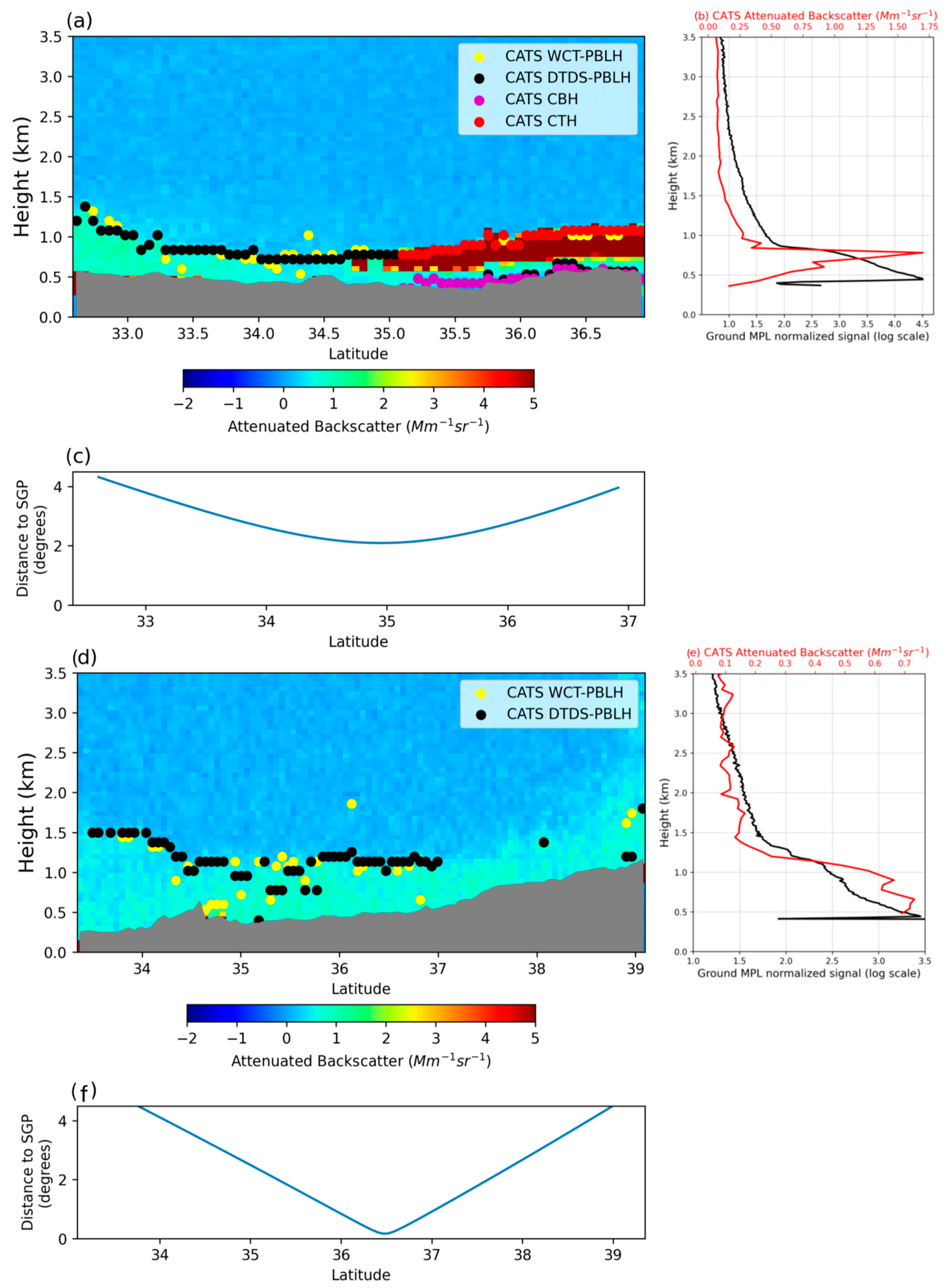
Figure 4 presents two examples of typical CATS samples within the grid box around the SGP site, one example showing a case with majority of retrievals classified as good and the other one with majority of mediate-quality. Figure 4c,f show the distance of CATS trajectory to the SGP site. Figure 4a depicts a distinct aerosol layer and a low-level cloud along the CATS track during 10 January 2016. That day, 80% of the CATS DTDS-PBLH retrievals were classified as good, and the remaining 20% were denoted as mediate. Black dots represent DTDS-PBLH, yellow dots represent the WCT-PBLH, and red dots indicate the Cloud Top Height (CTH). There is notable alignment between the aerosol layer top and the CTH. In Figure 4b, mean vertical profiles of attenuated backscatter are shown for the ground-based MPL (black) and CATS (red). Although not perfectly correlated, both signals exhibit a similar trend, detecting the aerosol layer top at approximately 0.9 km. A prominent disparity between the profiles is the heightened attenuation of the backscatter signal below the aerosol layer top observed in CATS data, and above the cloud base in the MPL data.
Figure 4d presents a case on 29 September 2016, when CATS passed directly over the SGP site. During this overpass, all PBLH retrievals were classified as 38% good and 62% as mediate. The similarity between the CATS backscatter profile and the MPL normalized backscatter signal is noteworthy, as shown in Figure 4e. Both profiles exhibit a distinct step in the backscatter signal at around 1.3 km, with a second step signal apparent at approximately 0.7 km in both datasets. It is worth noting for both examples how the DTDS-PBLH retrievals have higher vertical consistency and spatial continuity than the WCT-PBLH, which jumps between different levels. These examples highlight the consistency and reliability of CATS in capturing key features of the atmospheric boundary layer, reinforcing its utility for PBLH retrievals.
It’s crucial to distinguish between aerosol-based Planetary Boundary Layer Height (PBLH) retrievals from Lidar systems and thermodynamic-based PBLH retrievals using profiles such as those from radiosondes. While these estimations may align well under CBL conditions, they can diverge significantly during nocturnal periods. Aerosol-based PBLH retrievals at night typically reflect the top of the residual aerosol layer, whereas thermodynamic estimates signify the top of the stable layer. Nocturnal hours primarily feature SBLs, though NBL can also manifest, resulting in a closer agreement between aerosol-based and thermodynamic PBLH retrievals. The retrievals depicted in Figure 4a,d likely correspond to the residual layer.
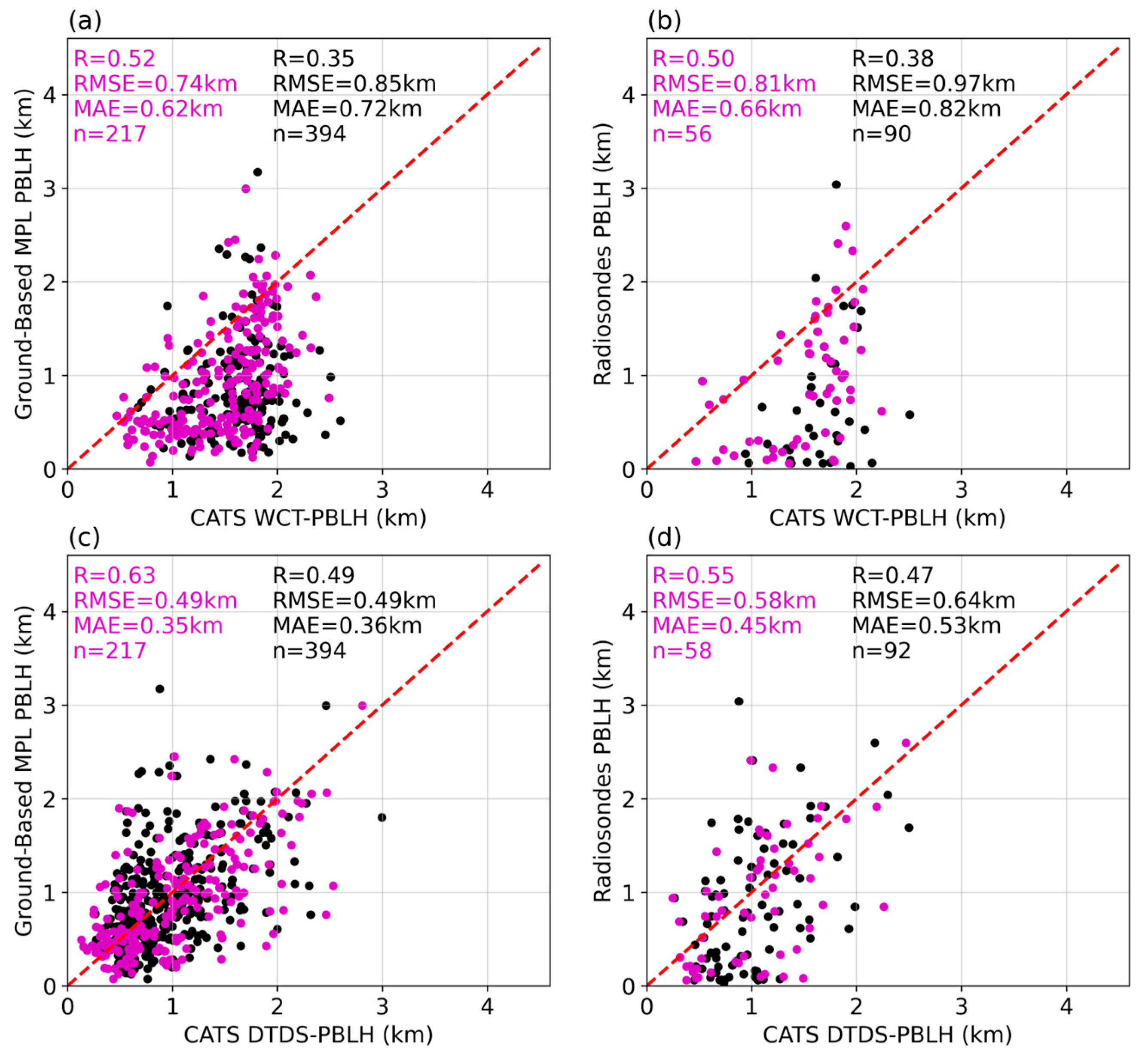
Comparisons of the traditional CATS WCT-PBLH retrievals with the ground-based MPL and PBLHs derived from local radiosondes demonstrate the limitations of the WCT method. In Figure 5a,b, we compare the PBLH estimates derived from CATS using the WCT method (CATS WCT-PBLH) with two different PBLH estimations. The first PBLH estimation is derived from ground-based lidar using the DTDS algorithm (ground-based DTDS-PBLH), while the second is derived from radiosondes (RS-PBLH) using the method of Liu and Liang [15]. These two PBLH products are more robust. Relative to them, the WCT-PBLH significantly overestimates the PBLH that is particularly pronounced for shallow boundary layers below 1 km, height above which the retrievals start to agree better. In contrast, the quality of new CATS DTDS PBLH retrievals is improved considerably, with smaller bias errors. Figure 5a,b include a quality control classification that arises from the DTDS algorithm and is not intrinsically incorporated into the WCT method. Therefore, the two samples shown in Figure 5a,b for the WCT respond to the need to make the WCT and DTDS results comparable.
In Figure 5, the sample size of the CATS DTDS-PBLH is significantly reduced even when using the entire CATS period as we have done in this study. This reduction is due to several factors. First, despite CATS operating for nearly three years, it did not pass through the SGP or ENA boxes on a daily basis. On average, CATS sampled the area around those sites 9 to 10 days per month. Second, on the days when CATS did pass through the box, PBLH retrieval was only feasible under clear sky conditions or single-layered cloudy situations with a cloud thickness equal to or lower than 1 km and a CTH lower than the maximum integration limit ( z t ) of the Haar function (see Section 3.2). Finally, the use of quality control flags in the algorithm also contributed to the reduction in sample size.
Given the top-down viewing geometry of spaceborne lidars, the overestimation of PBLHs derived from the traditional method likely results from the WCT function identifying the top of the residual layer or another elevated aerosol layer as the height of the maximum value in the WCT function. This disagreement between the CATS WCT-PBLH and the ground-based DTDS-PBLH retrievals is reflected in the statistical metrics with a correlation coefficient (R) of 0.52 and a large Root Mean Squared Error (RMSE) of 0.74 km. Compared to the RS-PBLH, the CATS WCT-PBLH has an R of 0.5 and an RMSE of 0.81 km when using the good-quality sample.
In a recent investigation by Li et al. [29], the performance of various traditional techniques, including the WCT, was evaluated, finding an average correlation of 0.6 and an RMSE of 0.9 km compared to radiosonde PBLH retrievals during clear sky conditions. However, our estimations differ from Li et al. [29] in several key aspects. First, they only investigated daytime conditions, while our study incorporates daytime and nighttime PBLH estimates. Second, Li et al. [29] provide statistical metrics from a global perspective, while our analysis focuses specifically on points crossing the SGP and the ENA site to permit satellite-ground comparisons. Finally, Li et al. [29] only considered cloud-free CATS profiles below 5 km, while this analysis includes clouds coupled with the surface, which corresponds to clouds lying below 4 km.
Our research findings highlight the significant improvements in terms of correlation and RMSE when using CATS PBLH retrievals with DTDS (CATS DTDS-PBLH) compared to the traditional WCT method, especially when considering only good-quality retrievals. Figure 5c,d provides a clear visual of these improvements. The DTDS product surpasses the WCT method with respect to comparisons against both the ground-based DTDS-PBLH and RS-PBLH estimate. When looking only at the good-quality retrievals, the correlation coefficient increased by nearly 21%, from 0.52 in the traditional method to 0.63 with the DTDS method, and the RMSE was reduced by almost 34%, decreasing from 0.74 km to 0.49 km. Similarly, when comparing CATS DTDS-PBLH to RS-PBLH (Figure 5d), the correlation increased by 10%, going from 0.5 to 0.55, and the RMSE was reduced by 29%, going from 0.81 km to 0.58 km. The superior performance of DTDS over the WCT method can be attributed to several factors, including the assessment of cloud-surface coupling, the treatment of each local maximum position as a potential PBLH, the use meteorological data in the retrieval algorithm, and the quality control assessment. Therefore, DTDS can be applied to spaceborne lidar datasets, not just point-based ground lidars, to evaluate regional, seasonal, and diurnal trends in PBLH, especially over continental regions.
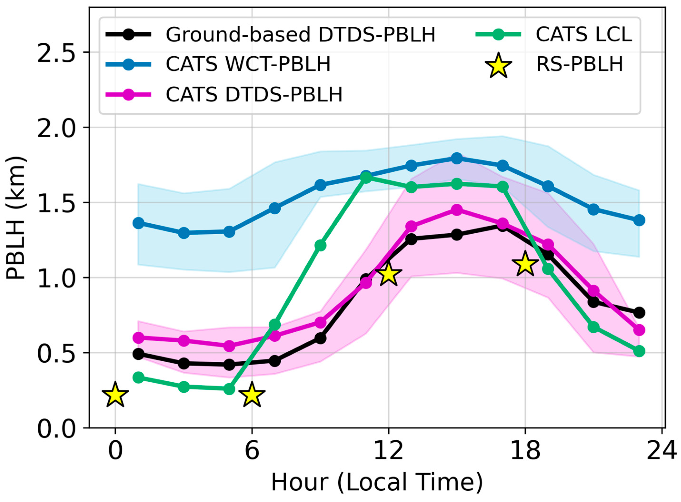
DTDS enables the analysis of the diurnal variability of the PBLH using spaceborne lidar data. Figure 6 presents the diurnal variations of the PBLH based on multiple methodologies with 2-h intervals, for good-quality retrievals only. Notably, the ground-based DTDS-PBLH and the CATS DTDS-PBLH align well at every hour, with overestimation of nearly 0.1 km at nighttime. Compared to the RS-PBLH, both CATS DTDS-PBLH and the ground-based DTDS-PBLH overestimate the RS-PBLH. However, such overestimation is small in the daytime and more significant at nighttime, reflecting the different nature of the PBLH retrieved by the thermodynamic and the substance approaches. Nevertheless, both CATS DTDS-PBLH and the ground-based DTDS-PBLH agree better with the RS-PBLH than the CATS WCT-PBLH does. The largest factor contributing to the higher proximity of DTDS retrievals to radiosonde retrievals at nighttime compared to the traditional WCT retrievals is the consideration of local meteorology through the use of the LCL. This parameter assists in the selection of the LMPs as the PBLH and in the assessment of the cloud-surface coupling.
Figure S3 in the supplementary material is similar to Figure 6, but it includes the mediate-quality retrievals. Overall, there is a good agreement between CATS DTDS-PBLH and surface-based PBLH retrievals using both good and mediate data points. Such an agreement is better when filtering the data to include only the best cases. However, due to the noisy nature of CATS data compared to ground-based lidar, and the uncertainties associated with using reanalysis for computing the LCL, many CATS DTDS-PBLH retrievals are classified as mediate quality. Therefore, for applications requiring a larger number of retrievals, such as case studies analysis, incorporating both good and mediate quality retrievals might be preferred.
Correctly estimating the nighttime PBL has been a key limitation of spaceborne lidars derived PBLHs using traditional approaches. The traditional CATS WCT-PBLH retrieval near the SGP site (Figure 6, blue) overestimates the PBLH by roughly 0.5 km in the afternoon and around 1 km in the night hours. Not only does the WCT product highly overestimate the PBLH, but it also varies a little throughout the day (~0.40 km), with a minimum of 1.3 km in the morning hours and maximum of 1.7 km in the afternoon). Contrary to the traditional method, the CATS DTDS-PBLH (Figure 6, purple/magenta) shows a much better agreement with the ground-based DTDS-PBLH and the RS-PBLH, with a shallow boundary layer at night that starts growing in the morning hours until it reaches its maximum peak (1.5 km) around 3:00 pm. While DTDS still overestimates the PBLH, this overestimation never exceeds 0.4 km, compared to the traditional WCT that overestimates the PBLH even by 1 km at nighttime. The shaded regions in Figure 6 for the CATS WCT-PBLH (blue) and the CATS DTDS-PBLH (purple) illustrate the interquartile range of both estimations. As shown, the ground-based DTDS-PBLH are located between the interquartile range of the CATS DTDS-PBLH, further proving the reliability of the DTDS method.
As stated previously, the inclusion of local meteorological information through the use of the LCL is the primary driver for the robust DTDS PBLH retrievals. The green line in Figure 6 illustrates the LCL computed using the meteorological data provided in the CATS data products. The LCL is a crucial parameter in DTDS as it plays a key role in assessing the cloud-surface coupling, particularly in addressing cloudy boundary layers. The meteorological data in CATS files is obtained from MERRA-2 reanalysis data interpolated to 5 km. In ideal conditions, the PBLH, CBH, and LCL should be located at the same altitudes. However, as Figure 6 shows, the computed LCL is consistently below the PBLH retrievals during nighttime and consistently above the PBLH during daytime. This discrepancy between the two retrievals is a potential source of error in the CATS DTDS-PBLH product. Errors in the computed LCL could lead to further errors in the cloud-surface coupling assessment and, consequently, errors in the PBLH retrieval during cloudy conditions. Therefore, the use of more accurate and precise meteorological data is essential for better assessments of the cloud-surface coupling and potentially increasing the robustness of the DTDS retrievals. This underscores the importance of collocated meteorological data and lidar information, not just as a desirable addition, but as a crucial requirement for future PBLH endeavors.
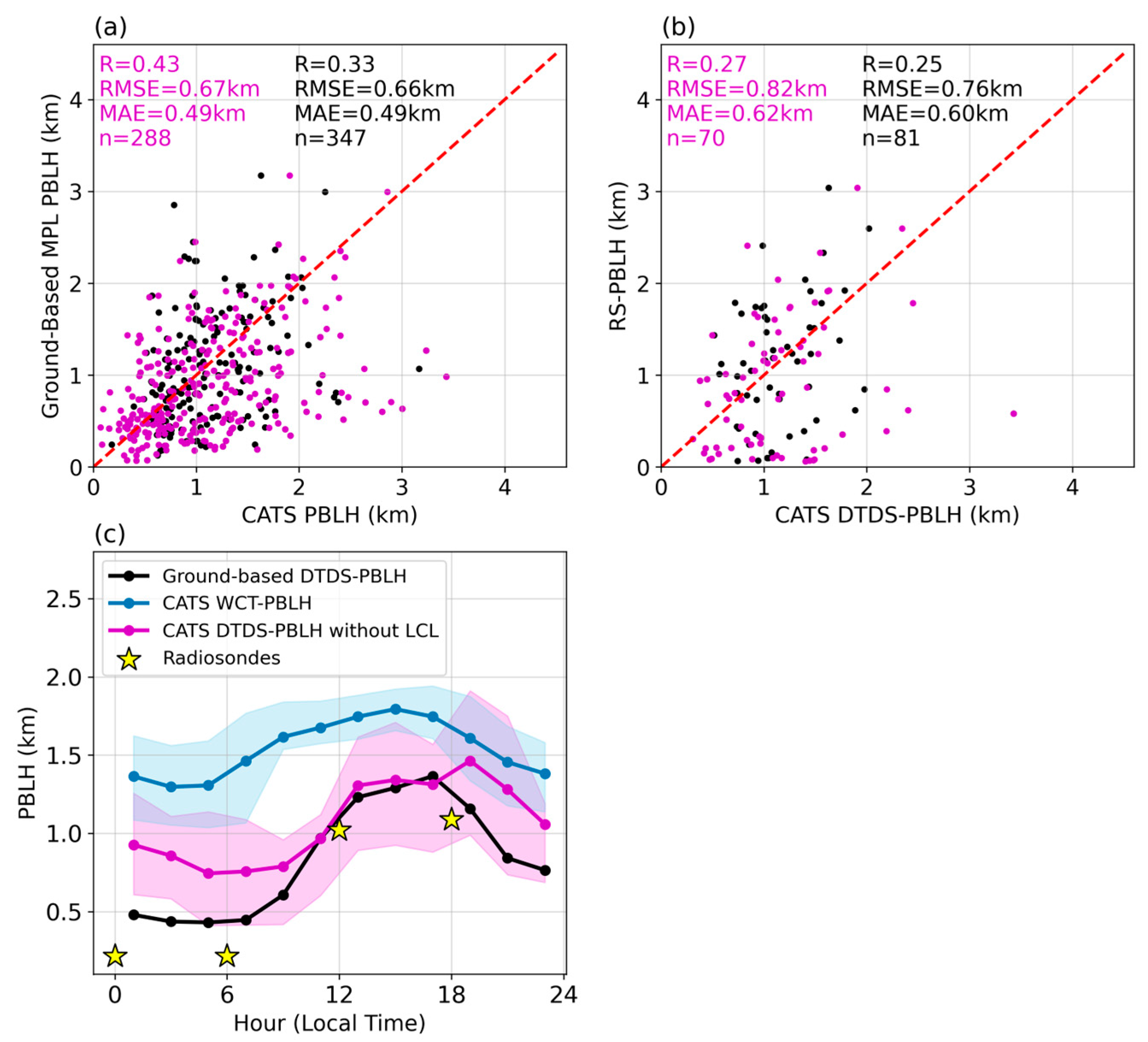
To investigate the effect of the LCL on the CATS DTDS-PBLH retrievals, we ran DTDS without the LCL conditionals in Figure 3, meaning the cloud-surface coupling was only based on the previous PBLH estimates. Figure 7 shows how the results of the CATS DTDS-PBLH without the LCL compare to two ground-based PBLHs. Figure 7c demonstrates that even without the LCL, DTDS can perform relatively well compared to ground-based MPL retrievals for daytime hours (10–17 LT). When analyzing the good-quality retrievals only, the correlation is equal to 0.43, and the RMSE is 0.67 km, both of which indicate worse performance compared to Figure 5c,d and Figure 6. Figure 7b shows the same comparison against radiosonde observations; overall, DTDS performance is highly compromised, with a 31% smaller correlation and 37% larger error.
The errors that occur when LCL is removed from DTDS are not evenly distributed throughout the day. Figure 7c shows the temporal variation of the PBLH computed without the LCL. In this case, the computed nighttime boundary layer is significantly overestimated, with differences as high as 0.5 km. However, it is worth noting that CATS DTDS-PBLH is still closer to the ground-based DTDS-PBLH and RS-PBLH retrievals than the traditional CATS WCT-PBLH estimates. Contrary to nighttime conditions, there is a better agreement between the CATS DTDS-PBLH, the ground-based DTDS-PBLH, and the RS-PBLH retrievals in the afternoon hours, suggesting that the use of LCL in the performance of DTDS is crucial during nighttime boundary layers when the SBL is difficult to detect using aerosol backscatter alone, favoring the determination of the PBLH at the residual layer. The combined use of the aerosol backscatter and meteorological information helps constrain the PBLH, providing better PBLH estimations than traditional algorithms. The results shown here highlight the accuracy of PBLH estimates using lidar data with collocated meteorological information, which can come from satellite and ground-based observations, and/or reanalysis data.

4.2. The Eastern North Atlantic (ENA)

The Eastern North Atlantic (ENA) site is known for its persistent low-level stratocumulus and cumulus clouds [45]. The arrangement of clouds in this area poses challenges for assessing cloud-surface coupling from space, especially when comparing ground-based and satellite lidar measurements. Ground-based sensors measure the base of the cumulus cloud layer, whereas satellite data senses the top of the stratocumulus layer. This difference has significant implications for evaluating cloud-surface coupling, which is critical for the performance of DTDS.
As observed in previous investigations [45,52,53,54], the stratus in this region corresponds to decoupled clouds, while the cumulus clouds lying on top of the mixed layer may be coupled to the PBLH. The base of coupled clouds, lying inside or on top of the mixed layer, serves as a great proxy to the PBLH. Decoupled clouds, however, have no direct contact with the PBLH and cannot be used to estimate it. Figure S2 compares the ground-based DTDS-PBLH with the RS-PBLH. As shown, both measurements have a good agreement with a correlation of 0.65 and an RMSE of 0.23 km. Generally, the ground-based DTDS-PBLH tends to underestimate the PBLH, probably because of the persistent presence of low-level clouds with bases below the PBLH. The strong signal of this cloud layer inhibits the lidar from seeing the atmosphere beyond the cloud base, and hence, DTDS will force the PBLH to be retrieved at the cloud base height. However, even with this limitation, the ground-based MPL senses the cumulus cloud layer that is coupled to the earth’s surface, providing a more reliable estimation of the PBLH. On the other hand, CATS, unable to see this cumulus coupled regime, senses exclusively the decoupled stratus clouds of this region. This limitation will directly impact the reliability of the PBLH estimations at this site using CATS observations.
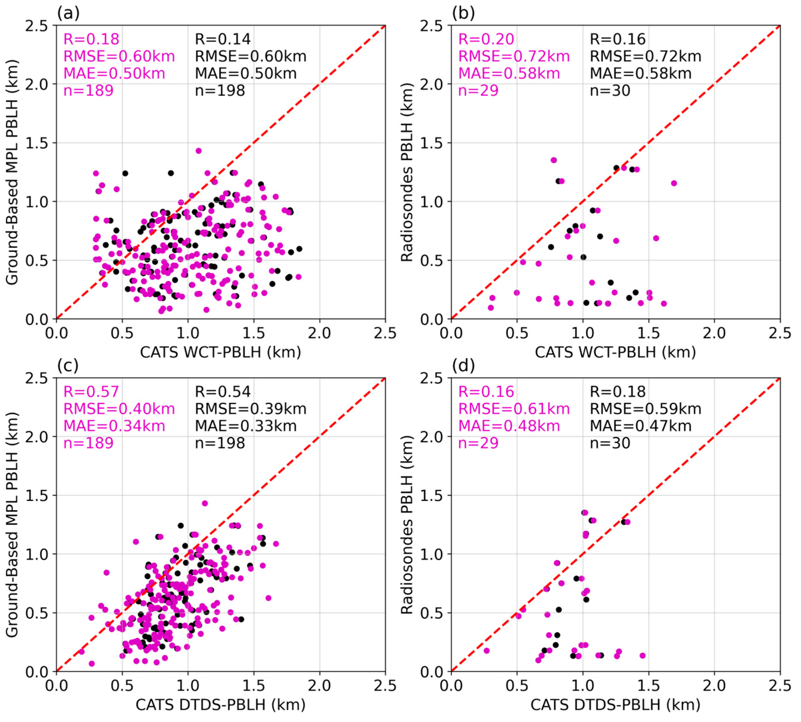
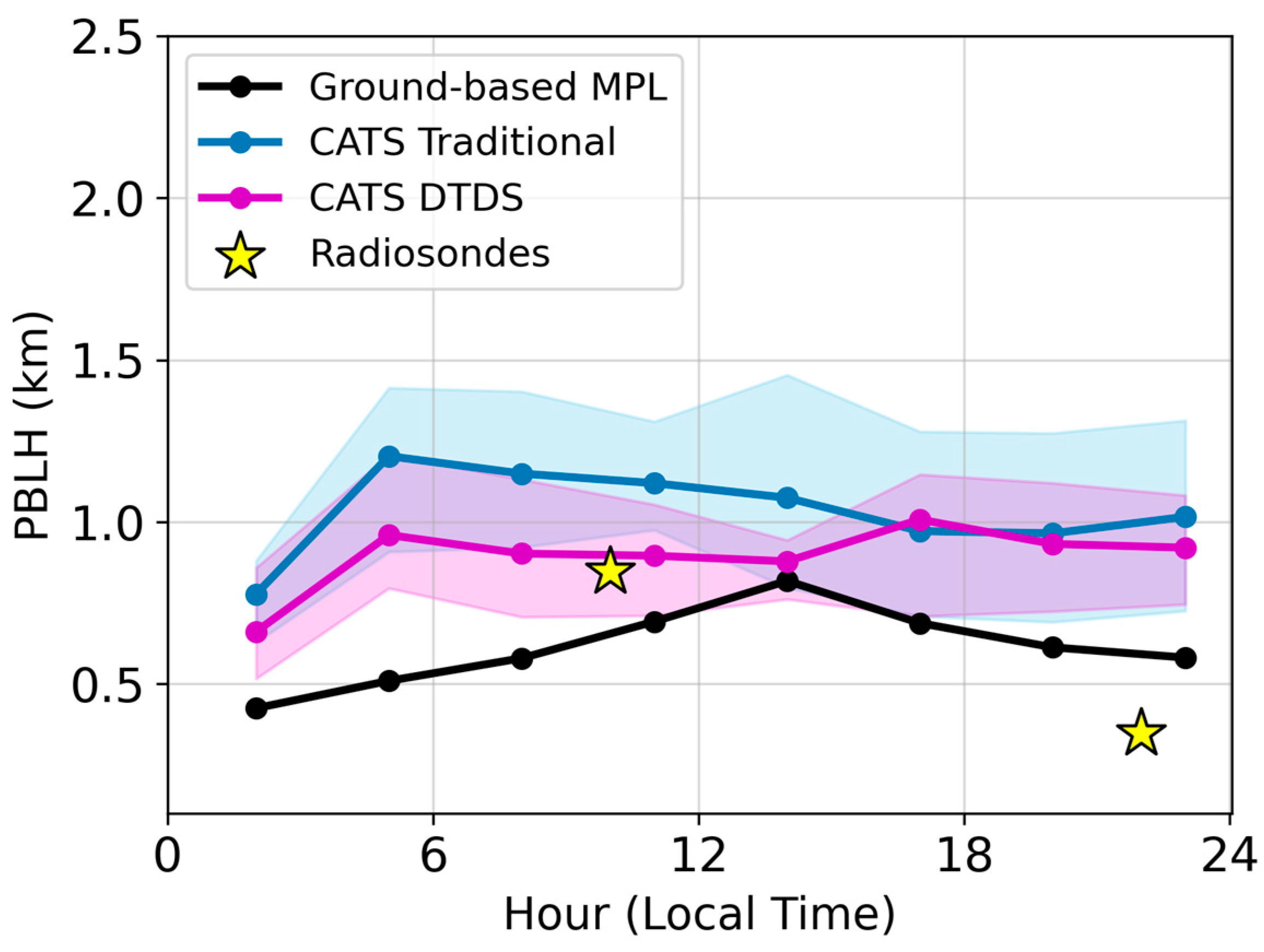
Figure 8a–d compares the ground-based DTDS-PBLH with the CATS DTDS-PBLH and CATS WCT-PBLH at the ENA site. The results show that CATS consistently overestimates the PBLH for both the WCT and DTDS products, with little dependence on the chosen quality control flag. The data also reveals a high degree of variability between the two CATS PBLH products and the two ground-based PBLHs. Considering only the retrievals classified as good-quality, the correlation between the CATS DTDS-PBLH and the ground-based DTDS-PBLH is 0.57, with an RMSE of 0.4 km. When compared to the radiosonde PBLH, the correlation coefficient is 0.16, with an RMSE of 0.61 km. For the CATS WCT-PBLH, the correlation coefficient with the ground-based DTDS-PBLH is 0.18, with an RMSE of 0.6 km, and with the radiosonde PBLH, the correlation coefficient is 0.2, with an RMSE of 0.72 km. Overall, these results suggest that the CATS DTDS-PBLH product performs better than traditional methods, even in complex environments. However, this study also highlights the limitations in the variability and magnitude of the CATS PBLH products, which are reflected in the diurnal temporal variability shown in Figure 9. The CATS DTDS-PBLH product consistently lies between 0.1 and 0.5 km above the ground-based product. The findings shown in Figure 8 and Figure 9 underscore the limitations of the CATS DTDS-PBLH product in accurately estimating the PBLH in different environmental conditions.
The difference in the performance of DTDS at retrieving the PBLH at the SGP site and the ENA site is a reflection of each site’s unique environmental conditions and complexities. The SGP site, situated over a midlatitude continental area, experiences a robust diurnal variation with a shallow boundary layer at nighttime and morning hours and a deep boundary layer in the afternoon. This pronounced diurnal variability is influenced, in part, by the lower heat capacity of soil that allows for larger diurnal variations of sensible heat flux and, hence, more significant variations in buoyancy fluxes and the boundary layer. The low-level clouds at the SGP site, which constitute a significant fraction of coupled boundary layer clouds, are another environmental factor that CATS can sense and DTDS can use to estimate the PBLH. In contrast, the ENA site, located in a marine environment, exhibits a subtle diurnal variability, with a shallow boundary layer that oscillates approximately 0.25 km over the diurnal cycle. This relatively constant boundary layer is influenced, in part, by the large heat capacity of the ocean that inhibits large fluctuations in the heat fluxes and the boundary layer. The complex cloud structure characterized by stratocumulus to cumulus transition is the main challenge when estimating the PBLH at this marine site, as it inhibits the correct assessment of the cloud-coupling regime. As mentioned, spaceborne lidar systems like CATS cannot measure the low-level cumulus clouds below the stratus layer, sensing mainly the top of the decoupled stratus with no information about the PBLH. As a result of the complex cloud structure at the ENA site, adjusting the PBLH estimates by adding or removing the lifting condensation level (LCL) does not correct the observed overestimations. Therefore, the LCL impact analysis was excluded for the ENA site.
To provide a deeper understanding of the diverse environments and cloud regimes at both SGP and ENA sites, Figure S4 presents the probability distribution of cloud fraction at both locations. The cloud fraction, a key indicator, was computed as the ratio between the low-level cloudy pixels vs. total pixels inside the CATS granule that crosses the 8° × 8° area around each site. Cloud fractions at SGP are notably lower than those at ENA. The lower cloud fraction suggests clear sky conditions with some cumulus clouds, while larger cloud fractions are associated with overcast conditions linked with stratus systems. The cloud fraction at ENA is a stark contrast to SGP, with a bimodal distribution featuring a first peak near 0.6 and a second peak above 0.9. These two peaks hint at a complex cloud structure, a feature that aligns with our expectations for a stratocumulus-to-cumulus transition region.

5. Summary

The Planetary Boundary Layer Height (PBLH) is a key parameter for depicting boundary layer characteristics, playing important roles in air quality, weather, and climate. Despite ample efforts and progresses have been made in estimating this quantity, global monitoring of PBH has been challenging, especially regarding its diurnal variation on a global scale. This may only be possible through the use of spaceborne instruments providing the vertical profiles of atmospheric quantities, such as lidars. This study uses the Cloud-Aerosol Transport System (CATS), a spaceborne Lidar aboard the ISS, that measured vertical profiles of atmospheric quantities between March 2015 and October 2017. The precessing inclined orbit of CATS enables the statistical resolution of the PBLH diurnal variability over regions in the tropics and mid-latitudes and over meteorological seasons. To leverage CATS’ dataset, we used the modified and refined Different Thermo-Dynamics Stability (DTDS) algorithm and applied machine learning denoising techniques for retrieving PBLH. The approach computes the PBLH using the traditional wavelet covariance transform function and a scheme for the assessment of the cloud-surface coupling. These characteristics allow DTDS to perform better under stable regimes, including nighttime conditions. In addition, machine learning denoising improved the detection of the PBLH during daytime conditions by increasing CATS’ daytime SNR.
The performance of CATS DTDS-PBLH differs drastically for the continental and marine sites, with the continental site characterized by relatively flat terrain with a high number of boundary layer clouds that help retrieve the PBLH. In contrast, the marine environment presents a complex cloud structure characterized by a mixture of stratocumulus overlying cumulus clouds, complicating the PBLH retrieval from space. DTDS, using retrievals flagged as good, consistently captured the diurnal variability of the PBLH for a continental mid-latitude site (ARM’s SGP site), having a robust correlation of 0.63 and an RMSE of 0.49 km when compared to ground-based DTDS-PBLH. When using mediate-quality retrievals, the R reduces to 0.49, whereas the RMSE stays the same. However, its performance is significantly worse in the marine environment, the ARM’s ENA site, where it exhibited a lower correlation of 0.57 and an RMSE of 0.4 km when compared to ground-based DTDS-PBLH for the good-quality retrievals.
The different environmental conditions and cloud structures of each site are also reflected in the different diurnal variabilities found in each region. In the case of the SGP site, we found a good agreement between the CATS DTDS-PBLH, the ground-based DTDS-PBLH, and the radiosonde PBLH. Each of them shows a shallow boundary layer at night that grows continuously after 6:00 am until reaching its maximum peak in the afternoon hours around 4:00 pm. Contrary to the CATS DTDS-PBLH, the traditional CATS WCT-PBLH highly overestimates the PBLH, especially during nighttime, when the residual layer strongly influences the retrieval. DTDS can better capture the nighttime boundary layer by considering each local maximum position of the covariance transform function as a potential PBLH and assessing the cloud-surface coupling. The latter requires a knowledge of the lifting condensation level, a parameter used to evaluate whether a cloud is coupled or decoupled to the earth’s surface. In this regard, any information pertaining LCL would help such as the atmospheric profiles from sounding sensors. Together with lidar backscatter signals, they help improve estimate PBLH over continental regions with meteorology similar to SGP.
In the case of the ENA site, the PBLH has a relatively shallow and constant diurnal variability, with values that oscillate less than 0.4 km throughout the day. In this site, both CATS DTDS-PBLH and CATS WCT-PBLH overestimate the PBLH during the entire day, primarily because of the viewing geometry of spaceborne lidars and the complex cloud structure of this site. Given complex meteorological regimes like ENA, getting a complete global perspective on the PBLH diurnal variability is still challenging, but much more hopeful over continents than oceans.
To our knowledge, there are few studies of PBLH and its diurnal variability that use a combination of spaceborne lidar and meteorological data as presented in this paper. There are several studies that have found the maximum PBLH during the afternoon hours over continental regions between 1.4 and 2.0 km. McGrath-Spangler and Denning [17], Palm et al. [28] and Li et al. [29] all used spaceborne lidar data and found PBLHs closer to 2.0 km in the US Great Plains, as the PBLH increases from east (~1.0 km) to the mountainous western states (~3.0 km). This study found a maximum value of 1.4 km over the SGP site, which is lower likely due to the differences in techniques. Those studies used WCT, vertical variance of the backscatter, or backscatter thresholds to determine the PBLH for each profile independent of spatial evolution. Furthermore, Li et al. [29] did not include profiles with clouds present below 5 km. This study employs DTDS, which includes both coupled clouds and meteorological information (i.e., the location of the LCL), as well as the spatial evolution of the PBLH along the satellite track. Thus, the PBLHs reported here are more comparable to recent studies using meteorological stations and/or radiosonde data, such as Zhang et al. [55] and Seidel et al. [56], which reported values of ~1.3 km over the US Great Plains, respectively. While PBLH estimates derived from lidar backscatter gradients and sounding data are both important to our overall knowledge of the PBL, they both have limitations for estimating the PBLH diurnal variability across the globe. Lidar backscatter gradients tend to provide the mixing layer height, which at night is more representative of the residual layer than the stable boundary layer, and sub-synchronous orbiting spaceborne sensors only provide 2 datapoints per day. Similarly, most radiosonde sites only launch at 00 and 12 UTC. In this study, we use spaceborne lidar data in combination with the DTDS method to replicate the pattern and magnitude of the diurnal cycle over the US Great Plains compared to a ground-based lidar (Figure 6) and previous studies such as Molod et al. [57] and Zhang et al. (2020) [55] that used wind profiler data and meteorological weather station data, respectively. Similar patterns and magnitudes of diurnal variability were also found in previous studies over other continental regions, such as Europe, using ground-based lidars and advanced PBLH detection techniques [58,59]. Thus, this study demonstrates that spaceborne backscatter measurements, in combination with thermodynamic profiles from passive sounders, can provide accurate estimates of PBLH and its diurnal variability over continental regions like the US Great Plains.

Supplementary Materials

The following supporting information can be downloaded at: https://www.mdpi.com/article/10.3390/rs16173252/s1, Figure S1: Kernel distribution estimates for the ground-based DTDS-PBLH and the RS-PBLH based on the Liu–Liang method using potential temperatures at the ARM SGP site between March 2015 and October 2017. The correlation coefficient (R), root-mean-square error (RMSE), and mean absolute error (MAE) are given in each panel. Dashed red lines correspond to 1:1 lines; Figure S2: Kernel distribution estimates for the ground-based DTDS-PBLH and the RS-PBLH based on the Liu–Liang method using potential temperatures at the ARM ENA site between March 2015 and October 2017. The correlation coefficient (R), root-mean-square error (RMSE), and mean absolute error (MAE) are given in each panel. Dashed red lines correspond to 1:1 lines; Figure S3: Temporal variations of the PBLH with 2 hours intervals for different instruments and methodologies. The black line corresponds to the ground-based MPL PBLH based on DTDS (ground-based DTDS-PBLH). The magenta line is the CATS PBLH estimated using the DTDS algorithm (CATS DTDS-PBLH) considering mediate and good-quality retrievals. The blue line is the CATS PBLH estimated using the traditional WCT method (CATS WCT-PBLH). Yellow stars are the radiosonde PBLH retrieved using the Liu and Liang method (RS-PBLH). The green line is the computed lifting condensation level (LCL) using the provided meteorological data in CATS files (CATS LCL).; Figure S4: Estimated cloud fractions at the (a) Southern Great Plains (SGP) and (b) the Eastern North Atlantic (ENA).

Author Contributions

Conceptualization, J.E.Y.; methodology, N.R.-H., T.S. and P.A.S.; software, N.R.-H., T.S. and P.A.S.; validation, N.R.-H.; formal analysis, N.R.-H.; investigation, N.R.-H.; resources, J.E.Y. and Z.L.; data curation, N.R.-H.; writing—original draft preparation, N.R.-H. and J.E.Y.; writing—review and editing, All authors; visualization, N.R.-H.; supervision, Z.L. and J.E.Y.; project administration, J.E.Y. and Z.L.; funding acquisition, J.E.Y. and Z.L. All authors have read and agreed to the published version of the manuscript.

Funding

This work was funded by internal NASA GSFC strategic science funds and the NASA Decadal Survey Incubation (DSI) program (NNH21ZDA001N-DSI). N.R and Z.L. are also supported by the Atmospheric System Research program of the Department of Energy (Grant DE-SC0022919) and by the US National Science Foundation (NSF) (Grant AGS2126098). T. Su is supported by the DOE Atmospheric System Research Science Focus Area THREAD project. Work at LLNL is performed under the auspices of the U.S. DOE by LLNL under Contract DE-AC52-07NA27344.

Data Availability Statement

The original data presented in the study are openly available in Zenodo at https://zenodo.org/records/13376582 (accessed on 26 August 2024). All ARM data are publicly available at the USA Department of Energy Atmospheric Radiation Measurement Data Center: https://www.arm.gov/capabilities/instruments/sonde (accessed on 26 August 2024).

Conflicts of Interest

The authors declare no conflicts of interest.

References

  1. Stull, R.B. An Introduction to Boundary Layer Meteorology; Springer Science & Business Media: Berlin, Germany, 1988; Volume 13. [Google Scholar]
  2. Kaimal, J.C.; Finnigan, J.J. Atmospheric Boundary Layer Flows: Their Structure and Measurement; Oxford University Press: Oxford, UK, 1994. [Google Scholar]
  3. Garratt, J.R. The Internal Boundary Layer—A Review. Bound. Layer Meteorol. 1990, 50, 171–203. [Google Scholar] [CrossRef]
  4. Caughey, S.J.; Palmer, S.G. Some Aspects of Turbulence Structure through the Depth of the Convective Boundary Layer. Q. J. R. Meteorol. Soc. 1979, 105, 811–827. [Google Scholar] [CrossRef]
  5. Holtslag, A.A.M.; Nieuwstadt, F.T.M. Scaling the Atmospheric Boundary Layer. Bound. Layer Meteorol. 1986, 36, 201–209. [Google Scholar] [CrossRef]
  6. Mahrt, L. Stratified Atmospheric Boundary Layers. Bound. Layer Meteorol. 1999, 90, 375–396. [Google Scholar] [CrossRef]
  7. Teixeira, J.; Piepmeier, J.R.; Nehrir, A.R.; Ao, C.O.; Chen, S.S.; Clayson, C.A.; Fridlind, A.M.; Lebsock, M.; McCarty, W.; Salmun, H.; et al. Toward a Global Planetary Boundary Layer Observing System: The NASA PBL Incubation Study Team Report. In Toward a Global Planetary Boundary Layer Observing System: The NASA PBL Incubation Study Team Report; NASA: Washington, DC, USA, 2021. [Google Scholar]
  8. Moeng, C.H.; Cotton, W.R.; Bretherton, C.; Chlond, A.; Khairoutdinov, M.; Krueger, S.; Lewellen, W.S.; MacVean, M.K.; Pasquier, J.R.M.; Rand, H.A.; et al. Simulation of a Stratocumulus-Topped Planetary Boundary Layer: Intercomparison among Different Numerical Codes. Bull. Am. Meteorol. Soc. 1996, 77, 261–278. [Google Scholar] [CrossRef]
  9. Santanello, J.A.; Dirmeyer, P.A.; Ferguson, C.R.; Findell, K.L.; Tawfik, A.B.; Berg, A.; Ek, M.; Gentine, P.; Guillod, B.P.; Van Heerwaarden, C.; et al. Land-Atmosphere Interactions the LoCo Perspective. Bull. Am. Meteorol. Soc. 2018, 99, 1253–1272. [Google Scholar] [CrossRef]
  10. Knote, C.; Tuccella, P.; Curci, G.; Emmons, L.; Orlando, J.J.; Madronich, S.; Baró, R.; Jiménez-Guerrero, P.; Luecken, D.; Hogrefe, C.; et al. Influence of the Choice of Gas-Phase Mechanism on Predictions of Key Gaseous Pollutants during the AQMEII Phase-2 Intercomparison. Atmos. Environ. 2015, 115, 553–568. [Google Scholar] [CrossRef]
  11. Li, Z.; Guo, J.; Ding, A.; Liao, H.; Liu, J.; Sun, Y.; Wang, T.; Xue, H.; Zhang, H.; Zhu, B. Aerosol and Boundary-Layer Interactions and Impact on Air Quality. Natl. Sci. Rev. 2017, 4, 810–833. [Google Scholar] [CrossRef]
  12. Hu, X.M.; Nielsen-Gammon, J.W.; Zhang, F. Evaluation of Three Planetary Boundary Layer Schemes in the WRF Model. J. Appl. Meteorol. Clim. 2010, 49, 1831–1844. [Google Scholar] [CrossRef]
  13. Lemone, M.A.; Angevine, W.M.; Bretherton, C.S.; Chen, F.; Dudhia, J.; Fedorovich, E.; Katsaros, K.B.; Lenschow, D.H.; Mahrt, L.; Patton, E.G.; et al. 100 Years of Progress in Boundary Layer Meteorology. Meteorol. Monogr. 2018, 59, 9.1–9.85. [Google Scholar] [CrossRef]
  14. Seidel, D.J.; Ao, C.O.; Li, K. Estimating Climatological Planetary Boundary Layer Heights from Radiosonde Observations: Comparison of Methods and Uncertainty Analysis. J. Geophys. Res. Atmos. 2010, 115, 16113. [Google Scholar] [CrossRef]
  15. Liu, S.; Liang, X.Z. Observed Diurnal Cycle Climatology of Planetary Boundary Layer Height. J. Clim. 2010, 23, 5790–5809. [Google Scholar] [CrossRef]
  16. Molod, A.; Salmun, H.; Dempsey, M. Estimating Planetary Boundary Layer Heights from NOAA Profiler Network Wind Profiler Data. J. Atmos. Ocean. Technol. 2015, 32, 1545–1561. [Google Scholar] [CrossRef]
  17. McGrath-Spangler, E.L.; Denning, A.S. Estimates of North American Summertime Planetary Boundary Layer Depths Derived from Space-Borne Lidar. J. Geophys. Res. Atmos. 2012, 117, 15101. [Google Scholar] [CrossRef]
  18. Herrera-Mejía, L.; Hoyos, C.D. Characterization of the Atmospheric Boundary Layer in a Narrow Tropical Valley Using Remote-Sensing and Radiosonde Observations and the WRF Model: The Aburrá Valley Case-Study. Q. J. R. Meteorol. Soc. 2019, 145, 2641–2665. [Google Scholar] [CrossRef]
  19. Dai, C.; Wang, Q.; Kalogiros, J.A.; Lenschow, D.H.; Gao, Z.; Zhou, M. Determining Boundary-Layer Height from Aircraft Measurements. Bound. Layer Meteorol. 2014, 152, 277–302. [Google Scholar] [CrossRef]
  20. Kalmus, P.; Ao, C.O.; Wang, K.N.; Manzi, M.P.; Teixeira, J. A High-Resolution Planetary Boundary Layer Height Seasonal Climatology from GNSS Radio Occultations. Remote Sens. Environ. 2022, 276, 113037. [Google Scholar] [CrossRef]
  21. Winker, D.M.; Hunt, W.H.; McGill, M.J. Initial Performance Assessment of CALIOP. Geophys. Res. Lett. 2007, 34, L19803. [Google Scholar] [CrossRef]
  22. Jordan, N.S.; Hoff, R.M.; Bacmeister, J.T. Validation of Goddard Earth Observing System-Version 5 MERRA Planetary Boundary Layer Heights Using CALIPSO. J. Geophys. Res. Atmos. 2010, 115, D24218. [Google Scholar] [CrossRef]
  23. Leventidou, E.; Zanis, P.; Balis, D.; Giannakaki, E.; Pytharoulis, I.; Amiridis, V. Factors Affecting the Comparisons of Planetary Boundary Layer Height Retrievals from CALIPSO, ECMWF and Radiosondes over Thessaloniki, Greece. Atmos. Environ. 2013, 74, 360–366. [Google Scholar] [CrossRef]
  24. Zhang, W.; Guo, J.; Miao, Y.; Liu, H.; Zhang, Y.; Li, Z.; Zhai, P. Planetary Boundary Layer Height from CALIOP Compared to Radiosonde over China. Atmos. Chem. Phys. 2016, 16, 9951–9963. [Google Scholar] [CrossRef]
  25. Su, T.; Li, J.; Li, C.; Xiang, P.; Lau, A.K.H.; Guo, J.; Yang, D.; Miao, Y. An Intercomparison of Long-Term Planetary Boundary Layer Heights Retrieved from CALIPSO, Ground-Based Lidar, and Radiosonde Measurements over Hong Kong. J. Geophys. Res. 2017, 122, 3929–3943. [Google Scholar] [CrossRef]
  26. Melfi, S.H.; Spinhirne, J.D.; Chou, S.-H.; Palm, S.P. Lidar Observations of Vertically Organized Convection in the Planetary Boundary Layer over the Ocean. J. Clim. Appl. Meteorol. 1985, 24, 806–821. [Google Scholar] [CrossRef]
  27. Yorks, J.E.; McGill, M.J.; Palm, S.P.; Hlavka, D.L.; Selmer, P.A.; Nowottnick, E.P.; Vaughan, M.A.; Rodier, S.D.; Hart, W.D. An Overview of the CATS Level 1 Processing Algorithms and Data Products. Geophys. Res. Lett. 2016, 43, 4632–4639. [Google Scholar] [CrossRef]
  28. Palm, S.P.; Selmer, P.; Yorks, J.; Nicholls, S.; Nowottnick, E. Planetary Boundary Layer Height Estimates From ICESat-2 and CATS Backscatter Measurements. Front. Remote Sens. 2021, 2, 716951. [Google Scholar] [CrossRef]
  29. Li, Y.; Li, J.; Xu, S.; Li, J.; He, J.; Huang, J. Diurnal Variation in the Near-Global Planetary Boundary Layer Height from Satellite-Based CATS Lidar: Retrieval, Evaluation, and Influencing Factors. Remote Sens. Environ. 2023, 299, 113847. [Google Scholar] [CrossRef]
  30. Su, T.; Li, Z.; Kahn, R. A New Method to Retrieve the Diurnal Variability of Planetary Boundary Layer Height from Lidar under Different Thermodynamic Stability Conditions. Remote Sens. Environ. 2019, 237, 111519. [Google Scholar] [CrossRef]
  31. Roldán-Henao, N.; Su, T.; Li, Z. Refining Planetary Boundary Layer Height Retrievals From Micropulse-Lidar at Multiple ARM Sites Around the World. J. Geophys. Res. Atmos. 2024, 129, e2023JD040207. [Google Scholar] [CrossRef]
  32. Noel, V.; Chepfer, H.; Chiriaco, M.; Yorks, J. The Diurnal Cycle of Cloud Profiles over Land and Ocean between 51°S and 51°N, Seen by the CATS Spaceborne Lidar from the International Space Station. Atmos. Chem. Phys. 2018, 18, 9457–9473. [Google Scholar] [CrossRef]
  33. Lee, L.; Zhang, J.; Reid, J.S.; Yorks, J.E. Investigation of CATS Aerosol Products and Application toward Global Diurnal Variation of Aerosols. Atmos. Chem. Phys. 2019, 19, 12687–12707. [Google Scholar] [CrossRef]
  34. Nowottnick, E.P.; Christian, K.E.; Yorks, J.E.; McGill, M.J.; Midzak, N.; Selmer, P.A.; Lu, Z.; Wang, J.; Salinas, S.V. Aerosol Detection from the Cloud–Aerosol Transport System on the International Space Station: Algorithm Overview and Implications for Diurnal Sampling. Atmosphere 2022, 13, 1439. [Google Scholar] [CrossRef]
  35. Pauly, R.M.; Yorks, J.E.; Hlavka, D.L.; McGill, M.J.; Amiridis, V.; Palm, S.P.; Rodier, S.D.; Vaughan, M.A.; Selmer, P.A.; Kupchock, A.W.; et al. Cloud-Aerosol Transport System (CATS) 1064&thinsp;Nm Calibration and Validation. Atmos. Meas. Tech. 2019, 12, 6241–6258. [Google Scholar] [CrossRef] [PubMed]
  36. Yorks, J.E.; Selmer, P.A.; Kupchock, A.; Nowottnick, E.P.; Christian, K.E.; Rusinek, D.; Dacic, N.; McGill, M.J. Aerosol and Cloud Detection Using Machine Learning Algorithms and Space-Based Lidar Data. Atmosphere 2021, 12, 606. [Google Scholar] [CrossRef]
  37. Su, T.; Zheng, Y.; Li, Z. Methodology to Determine the Coupling of Continental Clouds with Surface and Boundary Layer Height under Cloudy Conditions from Lidar and Meteorological Data. Atmos. Chem. Phys. 2022, 22, 1453–1466. [Google Scholar] [CrossRef]
  38. Flynn, D.; Shi, Y.; Lim, K.; Riihimaki, L. Cloud Type Classification (CLDTYPE) Value-Added Product. 2017. Available online: https://www.arm.gov/publications/tech_reports/doe-sc-arm-tr-200.pdf (accessed on 22 July 2024).
  39. Ritsche, M. ARM Surface Meteorology Systems Instrument Handbook; PNNL: Richland, WA, USA, 2011. [Google Scholar]
  40. Holdridge, D.; Ritsche, M.; Prell, J.; Coulter, R. Balloon-Borne Sounding System (SONDE) Handbook. 2011. Available online: https://www.arm.gov/capabilities/instruments/sonde (accessed on 26 August 2024).
  41. Sisterson, D.L.; Peppler, R.A.; Cress, T.S.; Lamb, P.J.; Turner, D.D. The ARM Southern Great Plains (SGP) Site. Meteorol. Monogr. 2016, 57, 6.1–6.14. [Google Scholar] [CrossRef]
  42. Islam, M.M.; Meskhidze, N.; Rasheeda Satheesh, A.; Petters, M.D. Turbulent Flux Measurements of the Near-Surface and Residual-Layer Small Particle Events. J. Geophys. Res. Atmos. 2022, 127, e2021JD036289. [Google Scholar] [CrossRef]
  43. Sengupta, M.; Clothiaux, E.E.; Ackerman, T.P. Climatology of Warm Boundary Layer Clouds at the ARM SGP Site and Their Comparison to Models. J. Clim. 2004, 17, 4760–4782. [Google Scholar] [CrossRef]
  44. Dong, X.; Xi, B.; Minnis, P. A Climatology of Midlatitude Continental Clouds from the ARM SGP Central Facility. Part II: Cloud Fraction and Surface Radiative Forcing. J. Clim. 2006, 19, 1765–1783. [Google Scholar] [CrossRef]
  45. Albrecht, B.A.; Bretherton, C.S.; Johnson, D.; Schubert, W.H.; Frisch, A.S. The Atlantic Stratocumulus Transition Experiment—ASTEX. Bull. Am. Meteorol. Soc. 1995, 76, 889–904. [Google Scholar] [CrossRef]
  46. Jia, F.; Wong, W.H.; Zeng, T. DDUNet: Dense Dense U-Net With Applications in Image Denoising. In Proceedings of the IEEE/CVF International Conference on Computer Vision (ICCV) Workshops, Virtual, 11–17 October 2021; pp. 354–364. [Google Scholar]
  47. Selmer, P.; Yorks, J.; Nowottnick, E.; Christian, K.; Cresanti, A. A Deep Learning Lidar Denoising Approach for Improving Atmospheric Feature Detection. Remote Sens. 2024, 16, 2735. [Google Scholar] [CrossRef]
  48. Davis, K.J.; Gamage, N.; Hagelberg, C.R.; Kiemle, C.; Lenschow, D.H.; Sullivan, P.P. An Objective Method for Deriving Atmospheric Structure from Airborne Lidar Observations. J. Atmos. Ocean. Technol. 2000, 17, 1455–1468. [Google Scholar] [CrossRef]
  49. Brooks, I.M. Finding Boundary Layer Top: Application of a Wavelet Covariance Transform to Lidar Backscatter Profiles. J. Atmos. Ocean. Technol. 2003, 20, 1092–1105. [Google Scholar] [CrossRef]
  50. Zhang, H.; Zhang, X.; Li, Q.; Cai, X.; Fan, S.; Song, Y.; Hu, F.; Che, H.; Quan, J.; Kang, L.; et al. Research Progress on Estimation of the Atmospheric Boundary Layer Height. J. Meteorol. Res. 2020, 34, 482–498. [Google Scholar] [CrossRef]
  51. Romps, D.M. Exact Expression for the Lifting Condensation Level. J. Atmos. Sci. 2017, 74, 3891–3900. [Google Scholar] [CrossRef]
  52. Zheng, Q.; Miller, M.A. Summertime Marine Boundary Layer Cloud, Thermodynamic, and Drizzle Morphology over the Eastern North Atlantic: A Four-Year Study. J. Clim. 2022, 35, 4805–4825. [Google Scholar] [CrossRef]
  53. Rémillard, J.; Tselioudis, G. Cloud Regime Variability over the Azores and Its Application to Climate Model Evaluation. J. Clim. 2015, 28, 9707–9720. [Google Scholar] [CrossRef]
  54. Jensen, M.P.; Ghate, V.P.; Wang, D.; Apoznanski, D.K.; Bartholomew, M.J.; Giangrande, S.E.; Johnson, K.L.; Thieman, M.M. Contrasting Characteristics of Open-and Closed-Cellular Stratocumulus Cloud in the Eastern North Atlantic. Atmos. Chem. Phys. 2021, 21, 14557–14571. [Google Scholar] [CrossRef]
  55. Zhang, Y.; Sun, K.; Gao, Z.; Pan, Z.; Shook, M.A.; Li, D. Diurnal Climatology of Planetary Boundary Layer Height Over the Contiguous United States Derived From AMDAR and Reanalysis Data. J. Geophys. Res. Atmos. 2020, 125, e2020JD032803. [Google Scholar] [CrossRef]
  56. Seidel, D.J.; Zhang, Y.; Beljaars, A.; Golaz, J.C.; Jacobson, A.R.; Medeiros, B. Climatology of the Planetary Boundary Layer over the Continental United States and Europe. J. Geophys. Res. Atmos. 2012, 117, D17106. [Google Scholar] [CrossRef]
  57. Molod, A.; Salmun, H.; Marquardt Collow, A.B. Annual Cycle of Planetary Boundary Layer Heights Estimated From Wind Profiler Network Data. J. Geophys. Res. Atmos. 2019, 124, 6207–6221. [Google Scholar] [CrossRef]
  58. De Bruine, M.; Apituley, A.; Donovan, D.P.; Baltink, H.K.; De Haij, M.J. Pathfinder: Applying Graph Theory to Consistent Tracking of Daytime Mixed Layer Height with Backscatter Lidar. Atmos. Meas. Tech. 2017, 10, 1893–1909. [Google Scholar] [CrossRef]
  59. Kambezidis, H.D.; Psiloglou, B.E.; Gavriil, A.; Petrinoli, K. Detection of Upper and Lower Planetary-boundary Layer Curves and Estimation of Their Heights from Ceilometer Observations under All-weather Conditions: Case of Athens, Greece. Remote Sens. 2021, 13, 2175. [Google Scholar] [CrossRef]
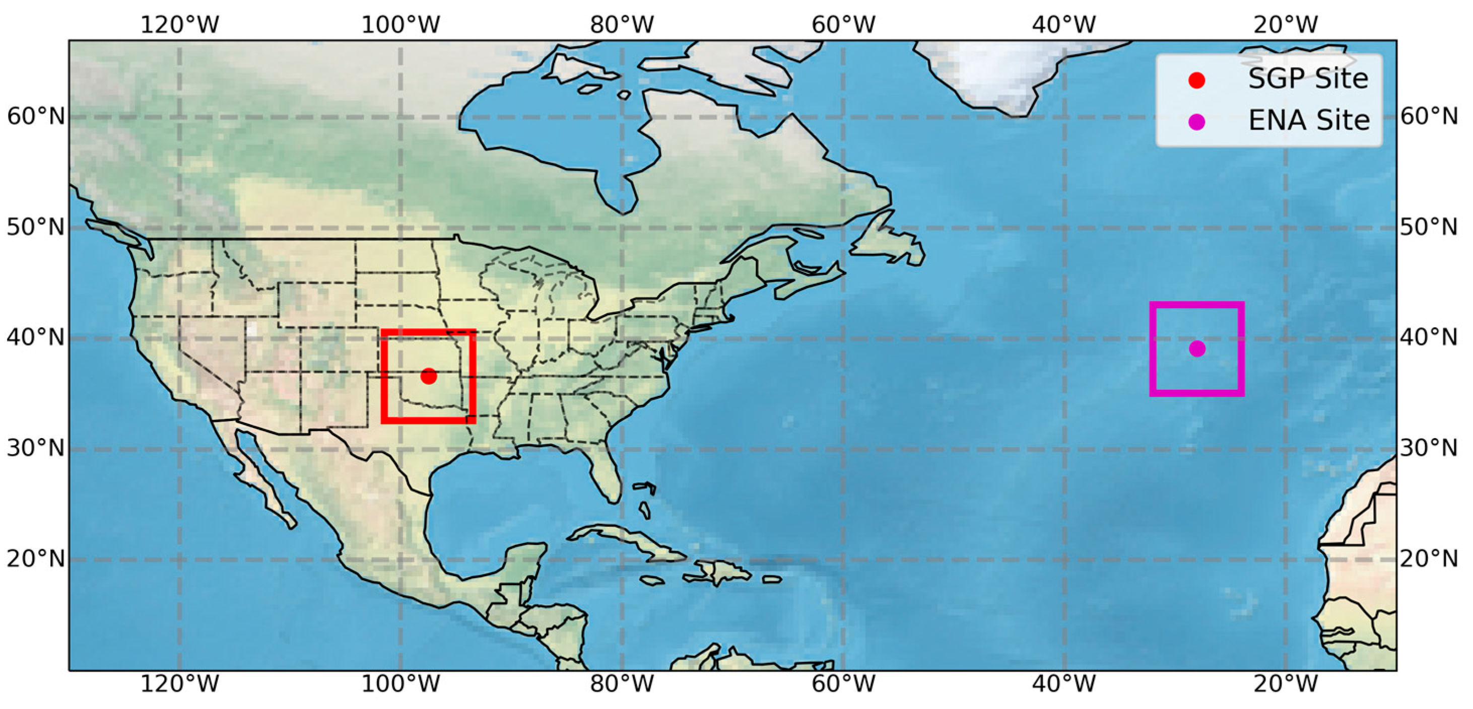
Figure 1. The locations of the two primary ARM sites used in this study. The red and magenta dots correspond to the Southern Great Plains (SGP) and Eastern North Atlantic (ENA) central locations, respectively. The squared boxes enclosing the dots correspond to the geographical region where CATS backscatter data is taken.
Remotesensing 16 03252 g001
Figure 2. (a) CATS Total Attenuated Backscatter and (b) CATS Denoised photon counts on 11 July 2015.
Remotesensing 16 03252 g002
Figure 3. Schematic diagram of the modified DTDS algorithm for the space-borne lidars. In this diagram, H(i) represents the Planetary Boundary Layer Height (PBLH) at each spatial interval i; CBH indicates the cloud base in single-layer clouds with a thickness smaller than 1 km. The PBLH selection identify the local maximum positions (LMPs) based on the spatial continuity. PBLH under the cloudy condition is determined by assessing cloud-surface coupling and utilizing information on the adjacent (nearby pixels) PBLH, cloud base height (CBH) and the lifted condensation level (LCL). Empirical parameters A1, A2, and A5 are set to 0.7, 0.2, and 1.1, respectively.
Remotesensing 16 03252 g003
Figure 4. (a) Example of the computed PBLH on 10 January 2016, the background colors correspond to the total attenuated backscatter measured by CATS over the Southern Great Plains (SGP). Black dots correspond to the Different Thermo-Dynamics Stability (DTDS) Planetary Boundary Layer Height (DTDS-PBLH), yellow dots are the wavelet covariant transform (WCT) PBLH (CATS WCT-PBLH), red dots are the Cloud Top Height (CTH), and magenta dots are the Cloud Base Height (CBH). (b) Average vertical profile of the attenuated backscatter measured by CATS (red line), and the ground-based Lidar backscatter profile measured at the same time as the CATS overpass (black line). (c) Distance of CATS to the SGP site in degrees. (df) same as (ac) but for 29 September 2016.
Remotesensing 16 03252 g004
Figure 5. (a) Scatter plots showing the relationship between the ground-based Micropulse DTDS-PBLH and CATS WCT-PBLH for samples classified as good quality only (magenta dots) and samples considered good and mediate (black dots) over the Southern Great Plains (SGP). The quality classification results from the DTDS algorithm and is not incorporated in the WCT method. Classifying the WCT dataset between good (magenta dots) and good and mediate (black dots) responds to the need to make the samples of both methodologies comparable. (b) same as (a) but comparing CATS WCT-PBLH with radiosonde PBLH retrievals. (c,d) same as (a,b) but for CATS DTDS-PBLH.
Remotesensing 16 03252 g005
Figure 6. Temporal variations of the PBLH with 2 h intervals for different instruments and methodologies over the Southern Great Plains (SGP). The black line corresponds to the ground-based MPL PBLH based on DTDS (ground-based DTDS-PBLH). The magenta line is the CATS PBLH estimated using the DTDS algorithm (CATS DTDS-PBLH) only considering good-quality retrievals. The blue line is the CATS PBLH estimated using the traditional WCT method (CATS WCT-PBLH). Yellow stars are the radiosonde PBLH retrieved using the Liu and Liang method (RS-PBLH). The green line is the computed lifting condensation level (LCL) using the provided meteorological data in CATS files (CATS LCL).
Remotesensing 16 03252 g006
Figure 7. (a,b) same as Figure 5c,d but without the use of the lifting condensation level (LCL) in the DTDS algorithm. (c) same as Figure 6 but without LCL in the DTDS algorithm.
Remotesensing 16 03252 g007
Figure 8. (a) Scatter plots showing the relationship between the ground-based Micropulse DTDS-PBLH and CATS WCT-PBLH for samples classified as good quality only (magenta dots) and samples considered good and mediate (black dots) at the Eastern North Atlantic (ENA) site. Notice that the quality classification results from the DTDS algorithm and is not incorporated in the WCT method. Classifying the WCT dataset between good (magenta dots) and good and mediate (black dots) responds to the need to make the samples of both methodologies comparable. (b) same as (a) but comparing CATS WCT-PBLH with radiosonde PBLH retrievals. (c,d) same as (a,b) but for CATS DTDS-PBLH.
Remotesensing 16 03252 g008
Figure 9. Temporal variations of the PBLH with 2 h intervals for different instruments and methodologies over the Eastern North Atlantic (ENA). The black line corresponds to the ground-based MPL PBLH based on DTDS. The magenta line is the CATS PBLH estimated using the DTDS algorithm (CATS DTDS-PBLH). The blue line is the CATS PBLH estimated using the WCT method (also called the traditional method here). Yellow stars are the radiosonde PBLH retrieved using the Liu and Liang method.
Remotesensing 16 03252 g009
Disclaimer/Publisher’s Note: The statements, opinions and data contained in all publications are solely those of the individual author(s) and contributor(s) and not of MDPI and/or the editor(s). MDPI and/or the editor(s) disclaim responsibility for any injury to people or property resulting from any ideas, methods, instructions or products referred to in the content.