Abstract
In the infrared remote sensing imaging system, the output of the detector is uneven, resulting in noticeable stripe noise in the image, which significantly reduces the image quality. Therefore, in response to the problem of establishing a variational model for the image globally and fixing the fractional order of the regularization term in the existing stripe noise removal algorithms based on model optimization, a stripe noise removal algorithm for infrared remote sensing images based on an adaptive weighted variable order model is proposed. In this algorithm, the vertical and approximate components containing stripe noise in the image are first separated through multi-level and multi-scale wavelet transform, and only these two components are processed; secondly, the global sparsity and the gradient sparsity of stripe noise and the variable order gradient sparsity of the information component are constrained by L1 norm, so as to establish the stripe noise removal model. The order of the fractional derivative is adaptively assigned to each pixel of the information component through local variance; then, an adaptive weight operator is introduced, which can assign different weights to the pixels in the variable order derivative of the information component on the basis of the image gradient information. Finally, through the ADMM algorithm, we can obtain the optimal solution of this model. The processing results of simulated and actual data indicate that the proposed algorithm performs well in all indexes and has obvious advantages in removing stripe noise and preserving image details.
1. Introduction
Infrared remote sensing images are widely applied in agriculture, environmental protection, meteorological prediction, and other fields. However, due to the inconsistency of the readout circuits of the detector in the infrared remote sensing imaging system, the readout circuits of different channels have different output amplification levels when the input response levels are the same, resulting in non-uniformity. This non-uniformity often manifests as stripe noise in the images, directly affecting the image quality and causing difficulties for subsequent image classification, image detail enhancement, and target recognition [1,2,3]. Therefore, for the sake of enhancing the quality of infrared remote sensing images, it is essential to study methods that can not only preserve image details but also remove the stripe noise effectively.
In recent years, researchers have proposed a large number of methods for stripe noise removal, which can be mainly categorized into the following four types:
1. Stripe noise removal methods based on filtering. This type of method essentially uses various filters to filter out noise and preserve edge texture information. In 2015, Cao et al. proposed a non-uniformity correction method that performed one-dimensional guided filtering in the horizontal and vertical directions to separate noise from the image [4]. In 2016, Li et al. proposed a method for reducing ghosting on the basis of a bilateral filter [5] and time-domain high-pass filter, which divided the image into three regions and used different adjustment factors for different regions. In 2021, Shao et al. proposed a method for removing stripe noise in infrared images [6]. This method applied the least squares method and one-dimensional gradient domain guided filtering to separate stripe noise in the high-frequency image. The filter-based methods are more effective in removing stripe noise with a periodic pattern, but no filter can perfectly accommodate the frequency of all stripe noise, and it is inevitable to filter out some image components containing information, which makes the obtained clean image lose some effective information or makes “artifacts” appear.
2. Stripe noise removal methods based on statistics. This kind of method mainly utilizes the grayscale statistical characteristics of the detector, that is, from a statistical perspective, it assumes that the response expectation and variance of all detectors are consistent, represented by histogram matching and moment matching. In 2013, Geng L. et al. proposed an adaptive constant statistical method that analyzed the statistical features of each pixel and used a mean filter to estimate the parameters of the detector [7]. In 2016, Gao et al. proposed a stripe denoising method based on the statistical features of an image histogram [8]. In this method, the differences between the centroids of the histogram of the entire image and each pixel were taken as the coarse correction coefficients, and the fine correction coefficients were obtained according to the correlation coefficients of the histogram and the coarse correction coefficients. In 2022, Yan et al. proposed a non-uniformity correction method on the basis of adaptive moving window moment matching [9]. This method adaptively controlled the width of the moving window by calculating the scene complexity of the image and the local scene complexity of the image within the window, and then calculated the correction gain and offset value of the image within the moving window. The statistically based stripe noise removal methods have simple algorithm structure and high computational efficiency, but they are prone to produce the “band effect” when facing complex scenes.
3. Stripe noise removal methods based on a neural network. The proposal of the neural network method utilized the mechanism of the human retina in capturing image information, and corrected each pixel according to the information in the field of view. In 2019, Guan et al. proposed an innovative wavelet deep neural network [10], which accurately estimated the noise according to the inherent features of stripe noise and the complementary information between different wavelet sub-band coefficients, and separated stripe noise and scene details more thoroughly through a special directional regularizer. In 2023, Huang et al. proposed a dual-denoising-driven convolutional neural network [11], which introduced two auxiliary variables corresponding to the denoised image and stripe noise, respectively, and used the U-shaped network for the denoising auxiliary variable and the residual CNN for the stripe auxiliary variable. The neural network-based method does not have much requirement for noise characteristics in terms of noise removal, but we need to focus on the “artifacts” problem of moving objects caused by the excessive iteration of these methods.
4. Stripe noise removal methods based on model optimization. This kind of method has achieved better results in all the research at present, making full use of the obvious features of stripe noise and image information, constructing a minimized energy function and completing the solution, ultimately obtaining the optimized denoised image. The most classical denoising model is the total variation (TV) regularization denoising model [12,13,14], which can effectively separate stripe noise without losing too much edge information. Because the TV model is non-convex, the solving process of this model is very difficult. Therefore, it can be equivalent to an optimization problem of solving the energy functional equation. In 2004, Farsiu et al. used the principles of L1 norm minimization and robust regularization to optimize the TV model, and obtained a BTV model that can handle different types of noise [15]. Subsequently, in 2011, Bouali M analyzed the structural properties of stripe noise [16] and obtained a rule: the gradient change of stripe noise in the direction perpendicular to the stripe was much greater than that in the direction parallel to the stripe, so the Unidirectional Total Variational model (UTV) was proposed. The optimal solution obtained by this model not only achieved the removal of stripe noise but also effectively protected the details. In this model, the use of the L1 norm could better protect the detail characteristics in actual information.
Although the first-order variational model has proved to be a highly effective denoising method, the resulting image often exhibits the undesirable “staircase effect” when dealing with severe irregular stripe noise, as shown in Figure 1.
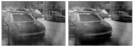
Figure 1.
Example images of “staircase effect”.
In order to overcome this drawback, in 2018, Song et al. proposed a weighted dual sparsity unidirectional variation (WDSUV) model based on the sparse characteristics of the spatial and gradient domains of stripe noise, which adopted different processing strategies for heavy stripe regions, extreme regions, and regular noise destruction regions [17]. In 2022, Song et al. proposed an enhanced prior combining double low-rank attributes, and combined this prior information with a total variational model, which not only effectively removed banding noise but also did not produce the “staircase effect” [18]. In addition, researchers have developed the high-order variational model. The well-known TVBH (TV bound Hessian) model [19] combined first-order variational and second-order variational, which not only achieved a better stripe noise removal effect but also prevented the “staircase effect” generated by the first-order variational model. In 2020, Yang et al. proposed a stripe removal model based on Schatten 1/2 norm regularization to describe the low rank of stripes, and based on UTV and unidirectional higher-order total variational (UHTV) regularization to ensure the smoothness of the underlying image and reduce the “staircase effect” [20]. Although the high-order variational model effectively overcomes the “staircase effect”, it uses a fixed fractional order for the image, making it difficult to make good adjustments to all parts of the image.
Therefore, aiming at the problems existing in the methods based on model optimization, this paper puts forward a stripe noise removal algorithm for infrared remote sensing images based on an adaptive weighted variable order model, so as to achieve an excellent denoising effect while preserving image details to the maximum extent.
The main contributions of this paper are summarized as follows:
(1) The stripe noise and useful image information are separated by multi-level and multi-scale wavelet transform, only the approximate and vertical components containing noise are processed, and the wavelet decomposition level is selected according to the information entropy of the approximate components, so as to prevent the loss of texture information caused by the excessive smoothing of pixels in the non-stripe area.
(2) A variable order model for removing stripe noise in infrared remote sensing images is proposed. Firstly, the L1 norm of the global sparsity of stripe noise and the L1 norm of the gradient sparsity of stripe noise in the vertical direction are taken as the regularization terms. Secondly, the L1 norm of the fractional derivative of the information component is taken as the fidelity term and, based on the local variance of the image, the order is automatically assigned to each pixel in the information component. The first-order variation is established for the pixel with small local variance and the second-order variation is established for the pixel with large local variance. Then, the denoising model is established through the regularization terms and fidelity term, which is solved by the ADMM algorithm [21,22]. In this way, the edge and texture information can be retained and the “staircase effect” can be avoided while removing stripe noise.
(3) A weight operator adapted to the image gradient is proposed, which adaptively gives different weights to the pixels in the edge area and the pixels in the texture area through the gradient information of the fractional derivative of the information component, achieving the effect of improving the ability of the model to protect image edge and texture information.
2. Materials and Methods
The algorithm proposed in this paper mainly includes five processes: In the first process, the wavelet transform is used to decompose the infrared remote sensing image containing stripe noise at multiple levels and scales, and stripe noise is concentrated in the approximate and vertical components of different levels. These two components are used to reconstruct the image through inverse wavelet transform, where the horizontal and diagonal components are set to zero, and the wavelet decomposition level is selected according to the information entropy of the approximate components. In the second process, a stripe noise removal model with fractional order adaptive selection according to local variance is established for the reconstructed noise image. In the third process, on the basis of the gradient values of the image information component, different weights are assigned to the edge and texture pixels. In the fourth process, the ADMM algorithm is utilized to solve this model to obtain the image containing clean multi-level vertical components and approximate components. In the fifth process, the multi-level vertical components and approximate components without stripe noise obtained in the fourth step and the horizontal and diagonal components obtained in the first step are reconstructed to obtain the clean image information component. Figure 2 shows the concrete flow of the algorithm.
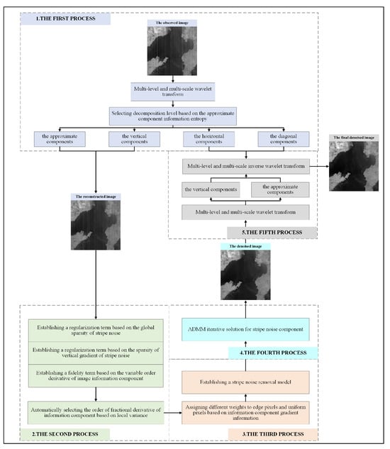
Figure 2.
The algorithm flowchart.
2.1. Obtaining the Noise Image through Multi-Level and Multi-Scale Wavelet Transform
After the decomposition of an infrared remote sensing image by multi-level and multi-scale wavelet transform, four sub-images of the horizontal, vertical, diagonal, and approximate components can be obtained [23,24].
2.1.1. Multi-Level and Multi-Scale Wavelet Decomposition
The decomposition of image by the wavelet transform is shown in the following equation:
where Y represents the observed noise image, n represents the wavelet decomposition level , , , , and represent the approximate components, horizontal components, vertical components, and diagonal components obtained by n-level wavelet decomposition, respectively, “.=” represents the decomposition and reconstruction relationship in the wavelet sense, and “.+” represents the set in the wavelet sense.
The formula for performing the first-level wavelet transform on the image with vertical stripe noise is shown in (1).
As can be seen from Figure 3, the relevant information of stripe noise along the vertical direction is distributed in the approximate and vertical components after the first-level wavelet decomposition, and there is no stripe noise in the horizontal and diagonal components. The frequency of stripe noise in the approximate component is lower than that in the vertical component. Therefore, stripe noise can be continuously separated from the image by performing the wavelet transform on the approximate component.

Figure 3.
First-level wavelet transform results.
The formula for performing the second-level wavelet transform on is as follows:
As can be seen from Figure 4, the intensity of stripe noise in the approximate and vertical components obtained from the second-level wavelet transform is significantly weaker than that in the first-level approximate and vertical components, but there is still a certain amount of stripe noise remaining in .

Figure 4.
Second-level wavelet transform results.
2.1.2. The Wavelet Reconstruction
After obtaining each component by wavelet transform, the image is reconstructed using the approximate component and the vertical detail components and through inverse wavelet transform. Since there is no stripe noise in the horizontal and diagonal detail components, these two components are set to zero in inverse wavelet transform. Due to the absence of vertical and diagonal components in the reconstructed image, it will be blurry, but stripe noise is basically restored.
The formula for the first-level inverse wavelet transform using and is as follows:
The formula for the second-level inverse wavelet transform using and is as follows:
2.1.3. The Selection of the Wavelet Decomposition Level
The higher the wavelet decomposition level, the more thorough the separation of stripe noise and other image details, but, at the same time, it can increase the time for image decomposition and reconstruction, which will reduce the processing efficiency of the algorithm. Therefore, selecting an appropriate decomposition level can better adapt to different types of images and noise patterns.
In this paper, a method of selecting wavelet decomposition level based on the approximate component information entropy is proposed. Information entropy is an index that can measure image complexity and uncertainty [25]. Generally, the higher the information entropy, the higher the complexity of the image, and the more information it contains, so a larger decomposition level is needed to capture this information. In order to select the optimal decomposition level, non-periodic stripe noise with noise ratio and intensity of 0.4 (−20∼20), 0.6 (−60∼60), and 0.8 (−100∼100) is added to Figure 5a, and the fixed wavelet basis function is used to perform multi-level and multi-scale decomposition on the image after adding noise, the information entropy of the decomposed approximate components is calculated, and the change in information entropy is observed with the increase in wavelet decomposition level. The graph is shown below, with the abscissa representing the decomposition level and the ordinate representing the information entropy of the approximate components:

Figure 5.
Inverse wavelet transform results.
From Figure 6, it can be seen that, as the decomposition level increases, the image is further subdivided into more sub-bands, and the detail information in the approximate components gradually decreases, resulting in a reduction in the information entropy. When the decomposition level increases to a certain extent, the approximate component contains very little detail information, so the information changes insignificantly after decomposition, and the information entropy tends to be stable. Moreover, when stripe noise in the image accounts for a relatively high proportion and the intensity is very large, a larger wavelet decomposition level is required to accurately capture the detail information. Therefore, this paper chooses the decomposition level that makes the approximate component information entropy curve tend to be stable as the optimal decomposition level, that is, the difference between the information entropy of the approximate component of the optimal level and the information entropy of the approximate component of the next level is less than 0.01, which can not only meet the denoising performance but also reduce the processing resources.
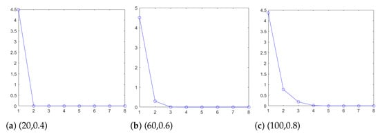
Figure 6.
The variation curves of approximate component information entropy with wavelet decomposition level.
2.2. Adaptive Weighted Variable Order Model
2.2.1. Problem Description
In the research on stripe noise removal algorithms based on model optimization, it is generally believed that stripe noise is additive noise [26,27,28], and the degradation process of the stripes can be expressed as follows:
, , and represent the original image, the image information component, and the stripe noise component, respectively. represents the pixel position. In this paper, model optimization is considered as the process of extracting the noise component from reconstructed by wavelet transform, which is transformed into the estimation problem of stripe noise. For the sake of calculation, Equation (6) is changed to matrix form:
2.2.2. Characteristics Description
In this section, the properties of the stripe noise component and the information component in structure and directionality are fully utilized, and the appropriate regularization constraints are used to describe them, so as to establish an estimation model about the noise component .
As shown in Figure 7c, in the infrared remote sensing image, stripe noise presents a column structure and accounts for a relatively small proportion of the image, which can be considered as a sparse matrix. L0 norm is most suitable for describing sparsity but, because of its non-convexity and difficult solvability [29,30], this paper uses L1 norm to constrain the global sparsity of stripe noise. L1 norm is a convex function that can be used as an approximation of L0 norm. From this, the regularization term is established as follows:
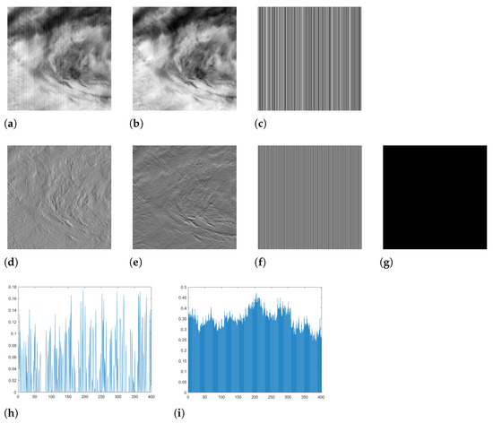
Figure 7.
Differences in various characteristics between the stripe noise component and the information component. (a) The original image. (b) The information component. (c) The stripe noise component. (d) The horizontal gradient of the information component. (e) The vertical gradient of the information component. (f) The horizontal gradient of the noise component. (g) The vertical gradient of the noise component. (h) The proportion of L1 norm of each column of the noise component to L1 norm of each column of the original image. (i) The proportion of L1 norm of the horizontal gradient in each row of the information component to L1 norm of the horizontal gradient in each row of the original image.
As shown in Figure 7e–h, the smoothness of the stripe noise component in the vertical direction is better than that of the information component, and L1 norm of each column of stripe noise only accounts for a very small part of L1 norm of each column of the original image. However, the smoothness of the gradient of the stripe noise component in the horizontal direction is not as good as that of the information component. Therefore, in order to distinguish these two components and better maintain the gradient sparsity of stripe noise in the vertical direction, the regularization term is established as follows:
where is a convolutional gradient operator along the vertical direction.
As shown in Figure 7d–f,i, in the horizontal direction, there are some obvious stripes in the gradient domain of stripe noise, while the gradient of the information component is smoother, and L1 norm of the gradient of each row of the information component also accounts for a small proportion in that of the original image. In addition, in the vertical direction, although the gradient of the information component is not as smooth as that of the information component, its gradient domain also has a certain sparsity. Therefore, utilizing these two features to establish the fidelity term,
Although the stripe noise removal model established by using only the first-order variation has a good denoising effect, it can cause the “staircase effect” in the edge area of the image. One way to avoid this effect to a certain extent is to use the second-order total variation, but it is easy to excessively smooth the image, and the fixed order of fractional derivative makes it difficult for the model to effectively process the edge area and uniform area of the image simultaneously. Therefore, it is necessary to adopt a variable order model, and Equation (10) is changed to the following:
where is the order of the fractional derivative, or .
2.2.3. Adaptive Selection of the Order of the Fractional Derivative
In this paper, we introduce a method to estimate the order of the fractional derivative based on local variance, which can adaptively assign fractional order to each pixel in the information component according to the size of local variance of the image. A small has a strong smoothing effect on the image, but it may overly emphasize the edges, resulting in a “staircase effect”. A large has a great ability to keep the edge and detail information. Therefore, in the uniform area, that is, the area with small variance, should be selected to protect the texture information and smooth stripe noise; in the edge area, that is, the area with large variance, should be chosen to maintain good image details and eliminate the “staircase effect”.
Firstly, the local variance of the image is calculated with the pixel as the center, the window size is , and the mean of the local variance of the entire image is obtained:
In Equation (12), is the mean gray value of all pixels in the window, and the fractional order is dynamically selected according to the relationship between and :
where T is the threshold that controls the value of .
2.2.4. A Weight Operator That Adapts to the Gradient of the Image
In infrared remote sensing images, the values of pixels located in the edge area of the image information component usually vary more than those of pixels located in the uniform area. Therefore, in the gradient plot of the information component, the pixel values located at the edge are larger than the other pixel values, as shown in Figure 8. When dealing with complex images that are heavily disturbed by stripe noise, the established regularization terms tend to weaken the contrast of the image edge and texture information. If the edge and texture structure are over-smoothed, the quality of the image will be greatly affected.
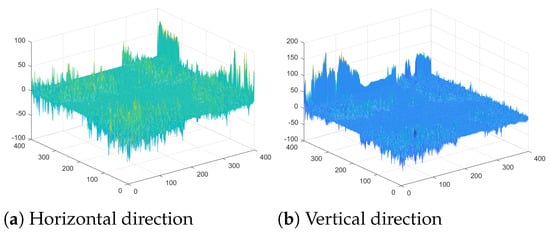
Figure 8.
Gradient plot of the image information component.
Therefore, in response to this issue, this paper proposes a weight operator that adapts to the image gradient; the weights assigned to each pixel are determined by the gradient plot of the estimated information component. Pixels with larger changes, namely edge area pixels, should be assigned smaller weights to weaken the sparsity constraints of these pixels. Conversely, pixels with smaller changes, namely uniform area pixels, should be assigned larger weights to enhance their sparsity constraints. Therefore, the weights need to be well aligned with the image texture information.
According to the principle that the weights are inversely proportional to the image texture, the obtained texture information is converted into weights, and the whole process is adaptive and efficient. The calculation formula is as follows:
where represents the absolute value operator and represents the threshold for controlling the weight range.
2.2.5. The Stripe Noise Removal Model
Combining the above three items, , , and , and the weight operator , the final model for removing stripe noise is as follows:
where , , and are regularization parameters used to balance various terms.
2.3. ADMM Optimization
The regularization terms containing L1 norm are not continuously differentiable, so the model cannot be solved by quadratic derivation. The essence of ADMM algorithm is to utilize block coordinate descent method to optimize the unconstrained optimization parts, which is one of the most effective algorithms to solve the model.
Firstly, three auxiliary variables, ,, and , are introduced to transform Formula (17) into a constrained optimization problem:
Formula (18) is transformed into an unconstrained equation through the Lagrange multiplier method:
where , , and are the ADMM penalty coefficients. When solving the equation, , , , , , and are separated.
(1) problem
The shrink operator is introduced to solve the problem, and :
(2) problem
(3) problem
(4) problem
The energy functional related to is as follows:
The closed-form solution of Equation (27) can be obtained by fast Fourier transform.
(5) , , problem
The substitution method is used directly to solve iteratively:
where k represents the number of iterations. After obtaining the noise component in the reconstructed noise image, the denoised image is obtained by .
The whole solution process of the model is summarized as Algorithm 1:
| Algorithm 1: The proposed algorithm. |
|
2.4. Obtaining the Final Denoised Image through Multi-Level and Multi-Scale Inverse Wavelet Transform
The model for stripe noise removal is adopted to process the reconstructed image. The reconstructed image does not contain the vertical and diagonal detail components, so the image information in these two directions will not be blurred while removing stripe noise. Since the image with non-periodic stripe noise with a noise ratio of 0.4 and an intensity of (−20∼20) is selected as experimental data in this section, as described in Section 2.1.3, the second-level wavelet decomposition is chosen. The denoised image is further decomposed by wavelet transform to obtain , , , , , , , and . At this point, stripe noise in the vertical detail components and approximate components has been removed, and , , and obtained in this section, and , , , and obtained in Section 2.1 are used to reconstruct image, which is the final denoised image.
The formula for the first-level inverse wavelet transform using , , , and is as follows:
The formula for the second-level inverse wavelet transform using , , , and is as follows:
3. Experiment and Analysis
For the sake of verifying the superiority and universality of the proposed algorithm, two kinds of experimental data are used in this experiment; one is the simulated infrared remote sensing image data with artificially added stripe noise, the other is the actual infrared remote sensing image data captured by the camera, both of which have a resolution of . In addition, the image processing effect of the proposed algorithm is compared with that of four advanced stripe noise removal algorithms in recent years: 1-D GF [4], ADOM [31], TSWEU [32], and LRDS [33]. In order to comprehensively evaluate the performance of each algorithm, in terms of quantification, the reference evaluation indexes PSNR and SSIM are utilized to measure the denoising effect of each algorithm on simulated infrared remote sensing images, and the non-reference evaluation indexes NR, MRD, and ID are utilized to measure the denoising effect of each algorithm on actual infrared remote sensing images. In terms of qualitative analysis, the row-average power spectral density curve is used to measure the striping ability of each algorithm. The computer hardware running platform for the experiment is 12th Gen Intel (R) Core (TM) i9-12900H@2.50 GHz and 32 GB RAM. The software platform is Matlab 2019b.
3.1. Experimental Setup
3.1.1. Evaluation Indexes
The reference evaluation indexes peak signal-to-noise ratio (PSNR) and structural similarity (SSIM) are defined as follows:
where MSE represents the mean square error and m is the number of bits per pixel.
In Formula (34), and , respectively, represent the average value of the current image X and the reference image Y, and , respectively, represent the variance of X and Y, represents the covariance of X and Y, and and are constants.
The higher the values of PSNR and SSIM, the better the image restoration.
The non-reference evaluation indexes noise reduction (NR) [34,35], mean relative deviation (MRD) [35,36], and image distortion (ID) [37,38] are defined as follows:
where and represent the power of the stripe noise frequency component in the input noise image and the denoised image, respectively. NR can reflect the overall performance of the image after striping and, the larger the NR, the better the image denoising effect.
where and represent the pixel values of the original image and the denoised image, respectively. is the size of the selected image area. MRD can reflect the image retention ability of areas less affected by stripes and, the smaller the MRD, the better the image retention ability.
where and represent the power spectrum of all frequencies of the original image and the information image after removing stripe noise, respectively. ID is used to measure the degree of image distortion after denoising and, the larger the ID, the better the image restoration effect.
3.1.2. Parameter Selection
Choosing appropriate parameters is crucial for the algorithm proposed in this paper, which involves three regularization parameters, , , and , and three penalty parameters, , , and , as well as the threshold T for controlling the value of and the threshold for controlling the range of . According to experience, is set in the range of [0.1, 1], is set in the range of [0.01, 0.1], is set in the range of [0.001, 0.1], , , and .
3.2. Ablation Experiment
For the sake of verifying the ability of to protect the edge and texture information of infrared remote sensing images, we process the same set of simulated image data with non-periodic stripe noise, which has a noise ratio of 0.4 and a noise intensity of (−20∼20), and quantitatively analyze the removal effect of the two stripe noise removal models without the weight operator and with the weight operator on stripe noise by PSNR and SSIM. The values marked in red and bold represent the optimal value of each index. Figure 9 and Table 1 show the experimental results:
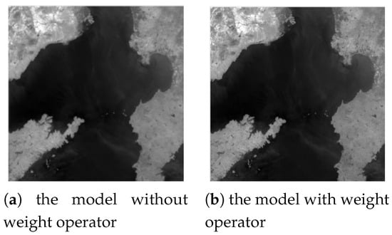
Figure 9.
Comparison of denoising effects between the two models.

Table 1.
PSNR values for the two models processing the same image.
It can be concluded that both models have removed stripe noise from the image but, compared with the stripe noise removal model without the weight operator, the image processed by the stripe noise removal model with the weight operator not only has clearer texture but also has better retention of detail information. Moreover, there are obvious advantages in PSNR and SSIM indexes, which fully demonstrates the effectiveness of the weight operator.
3.3. Results and Discussion
3.3.1. The Simulated Infrared Remote Sensing Image Data
In this section, three infrared remote sensing image scenes with different grayscale and contrast are selected for experimental comparison, namely the mountain image, the city image, and the desert image. In this paper, non-periodic stripe noise with a noise ratio of 0.6 and intensity of (−60∼60) is added to the images, which is relatively close to actual stripe noise. The actual information images obtained by each algorithm after striping are shown below. The small red and yellow boxes represent part of the image area, and the large red and yellow boxes represent part of the image area that has been enlarged.
The evaluation indexes PSNR and SSIM of the images processed by each algorithm are, respectively, shown in Table 2 and Table 3, and the optimal values of each index are highlighted in red and bold.

Table 2.
PSNR values of images processed by various denoising algorithms.

Table 3.
SSIM values of images processed by various denoising algorithms.
As shown in Figure 10, Figure 11 and Figure 12, when processing these three types of infrared remote sensing images, 1-D GF is unable to effectively distinguish and remove this irregular and high-intensity stripe noise, resulting in a significant amount of noise residue in the denoised images, and the red large square box indicates the location of the noise remnants. The PSNR and SSIM indexes also show that 1-D GF has the worst denoising effect. ADOM can remove all stripe noise; compared with 1-D GF, TSWEU, and LRDS, ADOM shows significant superiority in the PSNR index, but the SSIM index is lower than 0.997, indicating that the denoised images have not achieved good structural recovery, as shown in the yellow large square box, and the denoised images have the problem of attenuation of detail information. TSWEU is unable to remove all stripe noise, so that some noise remains in the denoised images. Moreover, the PSNR index is lower than 37 and the SSIM index is lower than 0.990, indicating that the detail information in some areas of the denoised images is blurred. Compared with 1-D GF and TSWEU, LRDS has a better effect on noise removal, with the PSNR index around 40 and the SSIM index greater than 0.996. Although the texture detail information of the images is effectively retained, a few stripes still remain. In this paper, as shown in the yellow large square box, the proposed algorithm not only completely removes stripe noise but also effectively preserves the edge texture information, and is superior to the previous four methods in PSNR and SSIM, which fully illustrates the advantages of this algorithm.
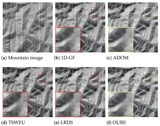
Figure 10.
Comparison of the denoising effects of each algorithm on mountain image.
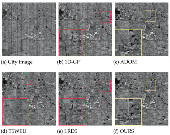
Figure 11.
Comparison of the denoising effects of each algorithm on city image.
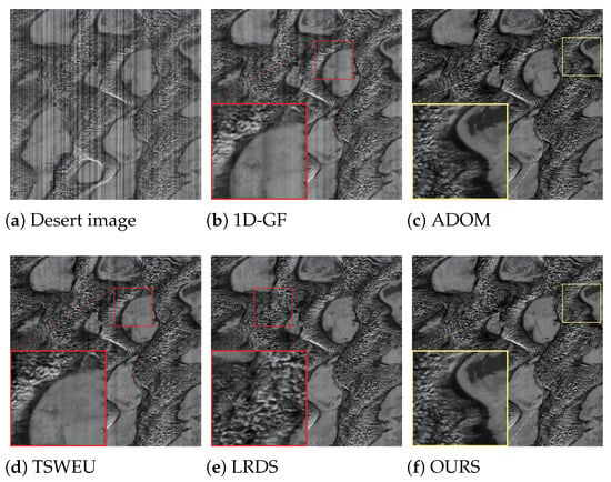
Figure 12.
Comparison of the denoising effects of each algorithm on desert image.
3.3.2. The Actual Infrared Remote Sensing Image Data
In this section, four actual infrared remote sensing image scenes with different grayscale and contrast are selected for experimental comparison, namely the mountain image, the building image, the cloud image, and the city image. The actual information images and the row average power spectral density graphs obtained before and after striping by each algorithm are shown below, with the abscissa as the normalized frequency and the ordinate as the average power spectrum of all rows; the blue and red curves represent the power spectral density of the original image and the denoised image, respectively. In the comparison graph of the row average power spectral density, the enlarged portion of the contrast curve is in the red rectangle box shown at the top. There are obvious blue spike pulses in the original image at a certain frequency, indicating that the original image contains some stripe noise. The reduction in red pulses after denoising can indicate that stripe noise has been eliminated to a certain extent, and the presence of smaller red pulses indicates that residual stripe noise has not been completely eliminated [39].
The non-evaluation indexes, NR, MRD, and ID, of the images processed by each algorithm are listed in Table 4. In this paper, five uniform regions of are selected to calculate the average MRD, and the optimal values of each index are highlighted in red and bold.

Table 4.
NR, MRD, and ID values of images processed by various denoising algorithms.
As shown in Figure 13, Figure 14, Figure 15 and Figure 16, compared with other methods, 1-D GF has the worst denoising effect. Although it preserves the edges and details, it is difficult to completely remove stripe noise in actual images. There is a certain amount of noise residue in the red square box. Moreover, small red pulses still present at the positions of larger blue pulses in the power spectral density graphs, which also indicates that some of the stripe noise has not been removed. ADOM performs well on the power spectral density graphs, with only very small spike pulses. ADOM can basically remove the majority of stripe noise, but there is a phenomenon of edge area pixels being excessively smoothed in the denoised images.
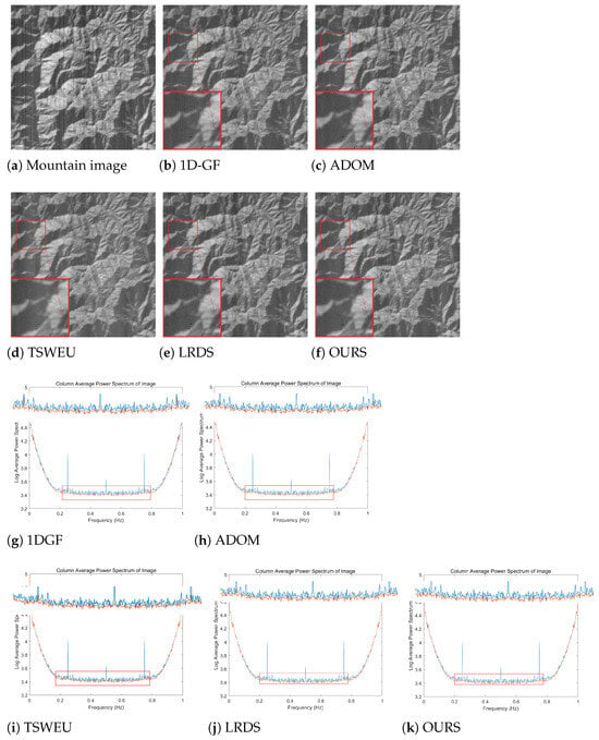
Figure 13.
Comparison of the denoising effects of each algorithm on mountain image.
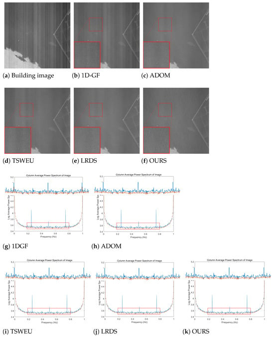
Figure 14.
Comparison of the denoising effects of each algorithm on building image.
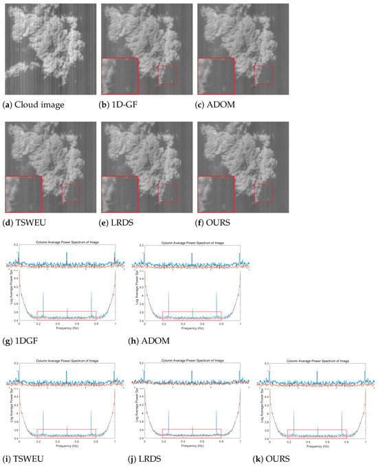
Figure 15.
Comparison of the denoising effects of each algorithm on cloud image.
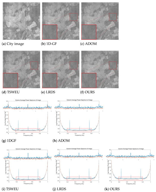
Figure 16.
Comparison of the denoising effects of each algorithm on city image.
Although TSWEU removes most of the stripe noise when processing the building image and cloud image, there are still some stripes remaining in the area marked by the red square box. When processing the mountain image and city image, the denoising effect of TSWEU is better than that of the first two images, with only a small number of stripes remaining. In addition, there are obvious red peak pulses in the power spectral density graphs of the four images. However, LRDS cannot take into account removing stripe noise and protecting image detail information at the same time; as a result, although the texture of the denoised images is clear, the stripe noise is not completely removed. There are still small red peak pulses in the power spectral density graphs. Although the proposed algorithm has a small part of the stripe noise left in the cloud image, it performs well on the other three images; the stripe noise has also been completely removed, and the red peak pulses on the power spectral density are relatively smaller compared with the other algorithms, effectively preserving the image edge and texture information. Therefore, considering the processing effect on four actual infrared remote sensing images, this algorithm is better than the first four methods in removing stripes, preserving image details, and power spectrum.
As shown in the table, the NR index of the proposed algorithm has the best results in all four images, indicating that, compared with the other four methods, it has excellent stripe removal ability.
In addition, the algorithm obtained the optimal MRD index on the mountain, cloud, and city images, showing a strong ability to maintain image detail information. Although the optimal MRD value is not obtained on the building image, the difference from the MRD value of ADOM is only 0.006%, indicating a good result. The algorithm in this paper achieves the optimal ID index on the mountain, building, and city images, but the ID index is higher than 0.95 on the cloud image, preserving the original information of images to the greatest extent. Through the qualitative and quantitative analysis of the denoised images, we can fully prove that this algorithm has excellent denoising ability and image information retention ability, and meets the satisfactory index requirements.
4. Conclusions
4.1. Summary
This paper proposes a stripe noise removal algorithm for infrared remote sensing images based on an adaptive weighted variable order model, which fully utilizes the multi-scale property of wavelet transform and the structural and directional differences between the stripe noise component and the information component to establish a variable order stripe noise removal model, and adaptively assigns the order of the fractional derivative and weights to each pixel of the information component according to the local variance and gradient information of the image, respectively. Finally, the ADMM algorithm is introduced to solve this model. The advantage of this algorithm lies in its ability to maximize the protection of texture information in the non-stripe area, while also taking into account the removal of stripe noise and the preservation of image edge information. The extensive experiments provided also demonstrate the effectiveness, superiority, and universality of this algorithm in stripe noise removal.
4.2. Limitations of the Proposed Algorithm
1. In infrared remote sensing images, there is not only vertical stripe noise, but also horizontal and oblique stripe noise. However, the algorithm in this paper does not fully consider the potential characteristics of oblique stripe noise, and can only be used to remove horizontal or vertical stripe noise.
2. In this paper, the average processing time of the proposed algorithm for the same type of actual infrared remote sensing images is calculated, and each type of images is not less than 100. The image processing time of the actual mountain and cloud types is 15 to 17 s, and the image processing time of the actual building and city types is 25 to 27 s. Compared with other comparison algorithms, the denoising model established in this paper is more complex and requires parameter adjustment calculation, resulting in a longer processing time.
4.3. Future Research Directions
1. Robustness to random noise. Although this algorithm has achieved remarkable results in removing stripe noise in infrared remote sensing images, random noise often affects image quality in practical applications. The model established in this paper is mainly aimed at removing stripe noise, and the processing of random noise is relatively insufficient. Therefore, future work can focus on optimizing the current model, mainly including studying the statistical characteristics and spatial distribution of random noise, optimizing the denoising model using these characteristics, and considering improving the regularization terms of the model and making adaptive selection of regularization parameters to enhance the robustness of the model to random noise. In addition, we will also study how to apply the improved denoising algorithm to a real-time image processing system to achieve the fast and effective removal of stripe noise and random noise.
2. Downstream tasks. For this paper, it will be an important research direction to further explore the influence of this stripe noise removal algorithm on various downstream tasks. For example, in the target detection task, we investigate whether the denoising algorithm in this paper can significantly improve the detection accuracy and recall rate; in the image segmentation task, we evaluate the effect of the denoising algorithm on the segmentation accuracy and edge detection. By conducting comprehensive tests on these tasks, we can understand how the denoising algorithm in this paper improves task performance and determine whether there is a performance bottleneck or room for improvement. In addition, different downstream tasks have different requirements for image quality. In the future, the adaptability of this denoising algorithm in specific tasks can be discussed, and whether it is necessary to make task-specific adjustments to the denoising model to optimize its performance in specific application scenarios can be considered. After that, we can further explore how to jointly optimize the denoising model in this paper and the downstream task model to ensure the stability and accuracy of the model in different tasks.
3. The utilization of multi-spectral information. In the study of removing stripe noise in infrared remote sensing images, we can explore how to fuse the multi-spectral image data of different bands in the future. Multi-spectral data provide rich spectral information, which can be combined to identify and remove noise more accurately and improve the image quality. In addition, we can study how to use the spectral features in multi-spectral images to improve the denoising algorithm. The introduction of spectral information helps to identify and process stripe noise more accurately, especially in the case of high spectral resolution, which can better distinguish noise from different sources. We can also develop denoising models suitable for multi-spectral data, which can deal with stripe noise in different spectral bands, enhance the overall image denoising effect, and achieve more comprehensive noise suppression.
Author Contributions
Conceptualization, L.H.; methodology, L.H.; software, L.H. and M.G.; validation, L.H. and M.L.; writing—original draft preparation, L.H.; writing—review and editing, L.H., T.N., M.L., H.Y. and M.G. All authors have read and agreed to the published version of the manuscript.
Funding
This work was supported by the National Natural Science Foundation of China (No. 62105328).
Data Availability Statement
Simulated infrared remote sensing image data used to support the research are available from the website https://github.com/JasonLi-UCAS/NIR-VIS-RS (accessed on 30 May 2024). Actual infrared remote sensing image data used to support the research are obtained from the AS-03 “Zhongdian Nongchuang” infrared remote sensing satellite.
Acknowledgments
The authors would like to thank the anonymous reviewers for their valuable comments.
Conflicts of Interest
The authors declare no conflicts of interest.
References
- Cao, Y.; He, Z.; Yang, J.; Cao, Y.; Yang, M.Y. Spatially adaptive column fixed-pattern noise correction in infrared imaging system using 1D horizontal differential statistics. IEEE Photonics J. 2017, 9, 7803513. [Google Scholar] [CrossRef]
- Liu, C.; Sui, X.; Gu, G.; Chen, Q. Shutterless non-uniformity correction for the long-term stability of an uncooled long-wave infrared camera. Meas. Sci. Technol. 2018, 29, 025402. [Google Scholar] [CrossRef]
- Chen, B.; Feng, X.; Wu, R.; Guo, Q.; Wang, X.; Ge, S. Adaptive wavelet filter with edge compensation for remote sensing image denoising. IEEE Access 2019, 7, 91966–91979. [Google Scholar] [CrossRef]
- Cao, Y.; Yang, M.Y.; Tisse, C.L. Effective strip noise removal for low-textured infrared images based on 1-D guided filtering. IEEE Trans. Circuits Syst. Video Technol. 2015, 26, 2176–2188. [Google Scholar] [CrossRef]
- Li, Z.; Shen, T.; Lou, S. Scene-based nonuniformity correction based on bilateral filter with reduced ghosting. Infrared Phys. Technol. 2016, 77, 360–365. [Google Scholar] [CrossRef]
- Shao, Y.; Sun, Y.; Zhao, M.; Chang, Y.; Zheng, Z.; Tian, C.; Zhang, Y. Infrared image stripe noise removing using least squares and gradient domain guided filtering. Infrared Phys. Technol. 2021, 119, 103968. [Google Scholar] [CrossRef]
- Geng, L.; Chen, Q.; Shi, F.; Wang, C.; Yu, X. An improvement for scene-based nonuniformity correction of infrared image sequences. In Proceedings of the International Symposium on Photoelectronic Detection and Imaging 2013: Infrared Imaging and Applications; SPIE: Bellingham, WA, USA, 2013; Volume 8907, pp. 669–677. [Google Scholar]
- Gao, H.t.; Liu, W.; He, H.y.; Zhang, B.x.; Jiang, C. De-striping for tdiccd remote sensing image based on statistical features of histogram. Int. Arch. Photogramm. Remote Sensing And Spat. Inf. Sci. 2016, 41, 311–316. [Google Scholar] [CrossRef]
- Yan, J.; Kang, Y.; Ni, Y.; Zhang, Y.; Fan, J.; Hu, X. Non-uniformity correction method of remote sensing images based on adaptive moving window moment matching. J. Imaging Sci. Technol. 2022, 66, 50502. [Google Scholar] [CrossRef]
- Guan, J.; Lai, R.; Xiong, A. Wavelet deep neural network for stripe noise removal. IEEE Access 2019, 7, 44544–44554. [Google Scholar] [CrossRef]
- Huang, Z.; Zhu, Z.; Wang, Z.; Li, X.; Xu, B.; Zhang, Y.; Fang, H. D3CNNs: Dual denoiser driven convolutional neural networks for mixed noise removal in remotely sensed images. Remote Sens. 2023, 15, 443. [Google Scholar] [CrossRef]
- Islam, M.R.; Xu, C.; Han, Y.; Ashfaq, R.A.R. A novel weighted variational model for image denoising. Int. J. Pattern Recognit. Artif. 2017, 31, 1754022. [Google Scholar] [CrossRef]
- Boutemedjet, A.; Deng, C.; Zhao, B. Edge-aware unidirectional total variation model for stripe non-uniformity correction. Sensors 2018, 18, 1164. [Google Scholar] [CrossRef] [PubMed]
- Zhang, Y.; Shao, Y.; Shen, J.; Lu, Y.; Zheng, Z.; Sidib, Y.; Yu, B. Infrared image impulse noise suppression using tensor robust principal component analysis and truncated total variation. Appl. Opt. 2021, 60, 4916–4929. [Google Scholar] [CrossRef] [PubMed]
- Farsiu, S.; Robinson, M.D.; Elad, M.; Milanfar, P. Fast and robust multiframe super resolution. IEEE Trans. Image Process. 2004, 13, 1327–1344. [Google Scholar] [CrossRef]
- Bouali, M.; Ladjal, S. Toward optimal destriping of MODIS data using a unidirectional variational model. IEEE Trans. Geosci. Remote Sens. 2011, 49, 2924–2935. [Google Scholar] [CrossRef]
- Song, Q.; Wang, Y.; Yan, X.; Gu, H. Remote sensing images stripe noise removal by double sparse regulation and region separation. Remote Sens. 2018, 10, 998. [Google Scholar] [CrossRef]
- Song, Q.; Huang, Z.; Ni, H.; Bai, K.; Li, Z. Remote sensing images destriping with an enhanced low-rank prior and total variation regulation. Signal, Image Video Process. 2022, 16, 1895–1903. [Google Scholar] [CrossRef]
- Papafitsoros, K.; Schönlieb, C.B. A combined first and second order variational approach for image reconstruction. J. Math. Imaging Vis. 2014, 48, 308–338. [Google Scholar] [CrossRef]
- Yang, J.H.; Zhao, X.L.; Ma, T.H.; Chen, Y.; Huang, T.Z.; Ding, M. Remote sensing images destriping using unidirectional hybrid total variation and nonconvex low-rank regularization. J. Comput. Appl. Math. 2020, 363, 124–144. [Google Scholar] [CrossRef]
- Xie, W.S.; Yang, Y.F.; Zhou, B. An ADMM algorithm for second-order TV-based MR image reconstruction. Numerical Algorithms 2014, 67, 827–843. [Google Scholar] [CrossRef]
- Xu, J.; Wang, N.; Xu, Z.; Xu, K. Weighted lp norm sparse error constraint based ADMM for image denoising. Math. Probl. Eng. 2019, 2019, 1262171. [Google Scholar] [CrossRef]
- Wang, E.; Jiang, P.; Hou, X.; Zhu, Y.; Peng, L. Infrared stripe correction algorithm based on wavelet analysis and gradient equalization. Appl. Sci. 2019, 9, 1993. [Google Scholar] [CrossRef]
- Wang, E.; Jiang, P.; Li, X.; Cao, H. Infrared stripe correction algorithm based on wavelet decomposition and total variation-guided filtering. J. Eur. Opt.-Soc.-Rapid Publ. 2020, 16, 1. [Google Scholar] [CrossRef]
- Liu, J.; Xu, M.; Xu, X.; Huang, Y. Nonreference image quality evaluation algorithm based on wavelet convolutional neural network and information entropy. Entropy 2019, 21, 1070. [Google Scholar] [CrossRef]
- Zhou, G.; Fang, H.; Yan, L.; Zhang, T.; Hu, J. Removal of stripe noise with spatially adaptive unidirectional total variation. Optik 2014, 125, 2756–2762. [Google Scholar] [CrossRef]
- Liu, X.; Lu, X.; Shen, H.; Yuan, Q.; Jiao, Y.; Zhang, L. Stripe noise separation and removal in remote sensing images by consideration of the global sparsity and local variational properties. IEEE Trans. Geosci. Remote Sens. 2016, 54, 3049–3060. [Google Scholar] [CrossRef]
- Kłosowski, M.; Sun, Y. Fixed pattern noise reduction and linearity improvement in time-mode CMOS image sensors. Sensors 2020, 20, 5921. [Google Scholar] [CrossRef]
- Guo, D.; Tu, Z.; Wang, J.; Xiao, M.; Du, X.; Qu, X. Salt and pepper noise removal with multi-class dictionary learning and l0 norm regularizations. Algorithms 2018, 12, 7. [Google Scholar] [CrossRef]
- Gu, Y.; Jin, J.; Mei, S. l_{0} norm constraint LMS algorithm for sparse system identification. IEEE Signal Process. Lett. 2009, 16, 774–777. [Google Scholar]
- Kim, N.; Han, S.S.; Jeong, C.S. ADOM: ADMM-based optimization model for stripe noise removal in remote sensing image. IEEE Access 2023, 11, 106587–106606. [Google Scholar] [CrossRef]
- Chang, Y.; Chen, M.; Yan, L.; Zhao, X.L.; Li, Y.; Zhong, S. Toward universal stripe removal via wavelet-based deep convolutional neural network. IEEE Trans. Geosci. Remote Sens. 2019, 58, 2880–2897. [Google Scholar] [CrossRef]
- Wu, X.; Qu, H.; Zheng, L.; Gao, T.; Zhang, Z. A remote sensing image destriping model based on low-rank and directional sparse constraint. Remote Sens. 2021, 13, 5126. [Google Scholar] [CrossRef]
- Shen, H.; Zhang, L. A MAP-based algorithm for destriping and inpainting of remotely sensed images. IEEE Trans. Geosci. Remote Sens. 2008, 47, 1492–1502. [Google Scholar] [CrossRef]
- Wang, J.L.; Huang, T.Z.; Ma, T.H.; Zhao, X.L.; Chen, Y. A sheared low-rank model for oblique stripe removal. Appl. Math. Comput. 2019, 360, 167–180. [Google Scholar] [CrossRef]
- Zeng, Q.; Qin, H.; Yan, X.; Yang, T. Fourier domain anomaly detection and spectral fusion for stripe noise removal of TIR imagery. Remote Sens. 2020, 12, 3714. [Google Scholar] [CrossRef]
- Li, Q.; Zhong, R.; Wang, Y. A method for the destriping of an orbita hyperspectral image with adaptive moment matching and unidirectional total variation. Remote Sens. 2019, 11, 2098. [Google Scholar] [CrossRef]
- Chen, Y.; Huang, T.Z.; Deng, L.J.; Zhao, X.L.; Wang, M. Group sparsity based regularization model for remote sensing image stripe noise removal. Neurocomputing 2017, 267, 95–106. [Google Scholar] [CrossRef]
- Wang, J.L.; Huang, T.Z.; Zhao, X.L.; Huang, J.; Ma, T.H.; Zheng, Y.B. Reweighted block sparsity regularization for remote sensing images destriping. IEEE J. Sel. Top. Appl. Earth Obs. Remote Sens. 2019, 12, 4951–4963. [Google Scholar] [CrossRef]
Disclaimer/Publisher’s Note: The statements, opinions and data contained in all publications are solely those of the individual author(s) and contributor(s) and not of MDPI and/or the editor(s). MDPI and/or the editor(s) disclaim responsibility for any injury to people or property resulting from any ideas, methods, instructions or products referred to in the content. |
© 2024 by the authors. Licensee MDPI, Basel, Switzerland. This article is an open access article distributed under the terms and conditions of the Creative Commons Attribution (CC BY) license (https://creativecommons.org/licenses/by/4.0/).