Abstract
As we take stock of the contemporary issue, remote sensing images are gradually advancing towards hyperspectral–high spatial resolution (H2) double-high images. However, high resolution produces serious spatial heterogeneity and spectral variability while improving image resolution, which increases the difficulty of feature recognition. So as to make the best of spectral and spatial features under an insufficient number of marking samples, we would like to achieve effective recognition and accurate classification of features in H2 images. In this paper, a cross-hop graph network for H2 image classification(H2-CHGN) is proposed. It is a two-branch network for deep feature extraction geared towards H2 images, consisting of a cross-hop graph attention network (CGAT) and a multiscale convolutional neural network (MCNN): the CGAT branch utilizes the superpixel information of H2 images to filter samples with high spatial relevance and designate them as the samples to be classified, then utilizes the cross-hop graph and attention mechanism to broaden the range of graph convolution to obtain more representative global features. As another branch, the MCNN uses dual convolutional kernels to extract features and fuse them at various scales while attaining pixel-level multi-scale local features by parallel cross connecting. Finally, the dual-channel attention mechanism is utilized for fusion to make image elements more prominent. This experiment on the classical dataset (Pavia University) and double-high (H2) datasets (WHU-Hi-LongKou and WHU-Hi-HongHu) shows that the H2-CHGN can be efficiently and competently used in H2 image classification. In detail, experimental results showcase superior performance, outpacing state-of-the-art methods by 0.75–2.16% in overall accuracy.
1. Introduction
Hyperspectral-high spatial resolution (H2) [1] images have finer spectral and spatial information [2] and can effectively distinguish spectrally similar objects by capturing subtle differences in continuous shape of the spectral features [3], realizing landmark recognition at the image element level [4]. H2 images have been widely used in environmental monitoring, pollution monitoring, geologic exploration, agricultural evaluation, etc. [5]. However, high dimensionality, a small number of labeled samples, spectral variability, and complex noise effects in H2 data [6] make it a great challenge to perform effective feature extraction, which leads to poor classification accuracy and low accuracy of feature recognition [7].
Traditional machine learning methods have a strong dependence on a priori knowledge and specialized knowledge when extracting features of an HSI, which makes it hard to extract deep features from an HSI [8]. Deep learning methods can better handle nonlinear data and outperform traditional machine learning-based feature extraction methods [9]. Convolutional neural networks (CNNs) [10] are good at extracting effective spectral spatial features from HSIs. Zhong et al. [11] operated directly on an original HSI and designed an end-to-end spectral spatial residual network (SSRN) using spectral and spatial residual blocks. Roy et al. [12] constructed a model called HybridSN by concatenating a 2D-CNN and a 3D-CNN to maximize accuracy. However, these methods also exhibit complex structures and high computational requirements [13]. Recently, transformers [14] have had good performance in processing HS data due to their self-self attention mechanism. Hong et al. [15]. proposed a novel network called SpectralFormer, which learns local spectral features from multiple neighboring bands at each coding location. Nonetheless, the transformers-based networks, e.g., ViT [16], inevitably experience a degradation in performance when processing HSI data [17]. Johnson et al. [18] proposed a neuro-fuzzy modeling method for constructing a fitness predictive model. Zhao et al. [19] proposed a new shuffle Net-CA-SSD lightweight network. Li et al. [20] proposed a variational autoencoder, GAN, for fault classification. Yu Li et al. [21] proposed a distillation-constrained prototype representation network for image classification. Bhosle et al. [22] proposed a deep learning CNN model for digit recognition. Sun et al. [23] proposed a deep learning data generation method for predicting ice resistance. Wang et al. [24] proposed a spatio-temporal deep learning model for predicting streamflow. Shao et al. [25] proposed a task-supervised ANIL for fault classification. Dong et al. [26] designed a hybrid model with a support vector machine and a gate recurrent unit. Dong et al. [27] designed a region-based convolutional neural network for epigraphical images. Zhao et al. [28] designed a interpretable dynamic inference system based on fuzzy broad learning. Yan et al. [29] designed a lightweight framework using separable multiscale convolution and broadcast self-attention. Wang et al. [30] designed a deep learning interpretable model with multi-source data fusion. Li et al. [31] proposed an adaptive weighted ensemble clustering method. Li et al. [32] proposed an automatic assessment method for depression symptoms. Li et al. [33] proposed an optimization-based federated learning for non-IID data. Xu et al. [34] proposed an ensemble clustering method based on structure information. Li et al. [35] proposed a deep convolutional neural network for automatic diagnosis of depression.
Deep learning-based feature extraction methods for HSIs are widely used because they can better extract the deep features of the image. Traditional convolutional neural networks (CNNs) [10] need to be trained with a massive number of labeled samples and have a high training time complexity. Graph Convolutional Neural Networks (GCNs) [36] can handle arbitrary structural data, adaptively learn parameters according to specific feature types, and optimize these parameters, which improves a model’s recognition performance in different feature types compared to traditional CNNs [37]. Hong et al. [3] proposed a miniGCN to reduce computation cost and realize the complementary positive aspect between a CNN and a GCN in a small batch. However, pixel-based feature extraction methods generate high-dimensional feature vectors and extract a large amount of redundant information. Therefore, in order to extract features more efficiently, researchers have introduced superpixels for use instead of pixels. Sellars et al. proposed a semi-supervised method (SGL) [38] that combines superpixels with graphical representations and pure-graph classifiers to greatly reduce the computational overhead. Sheng et al. [39] designed a multi-scale dynamic graph-based network (MDGCN), exploiting the multi-scale information with dynamic transformation. To enhance the computational efficiency and speed up the training process, Li et al. [40] designed a new symmetric graph metric learning (SGML) model by introducing a symmetry mechanism, which mitigates the spectral variability through symmetry mechanisms. Although the above methods utilize superpixels instead of pixels to reduce the computational complexity, these methods can only generate features at the superpixel level and fail to take into account subtle features within each superpixel during the spectral feature extraction process. Consequently, classification maps generated by GCNs are sensitive to over-smoothing and produce false boundaries between classes [17]. To overcome this problem, Liu et al. [41] proposed a heterogeneous deep network (CEGCN) that utilizes CNNs to complement the superpixel-level features of GCNs by generating local pixel-level features. Moreover, graph encoders and decoders are proposed to solve the incompatibility between CNNs and GCN data. Based on the above idea, the Multi-layer Superpixel Structured Graph U-Net (MSSG-UNet) [42], which gradually extracts varied scale features from coarse to fine and performs feature fusion, was generated. Meanwhile, in order to better utilize neighboring nodes to prevent information loss, [36] proposed the graph attention network (GAT), which uses k-nearest neighbors to find the adjacency matrix and compute the weights of different nodes. Dong et al. [43] used weighted feature fusion of a CNN and a GAT. Ding et al. [44] designed a fusion network (MFGCN) [45] and a multi-scale receptive field graph attention neural network (MRGAT). The above improved GCNs and enabled a more comprehensive use of spatial and spectral features by reconfiguring the adjacency matrices; however, converting the connections of the nodes may present superfluous information and degrade the classification performance. Xue et al. designed a multihop GCN using different branches and different hopping graphs [46], which aggregates multiscale contextual information by hopping. Zhou et al. proposed a fusion network with attention multi-hop graph and multi-scale convolutional (AMGCFN) [47]. Xiao et al. [48] proposed a privacy-preserving federated learning system in IIoT. Tao et al. [49] proposed a memory-guided population stage-wise control spherical search algorithm. However, the above networks are complex in structure and inefficient in model training. Some new methods have been proposed in recent years [50,51,52,53,54,55,56,57,58,59], which can be used to optimize these models.
Aimed at solving the above problems in extracting and classifying features from HSIs, such as the inconsistency of superpixel segmentation processing for similar feature classification, the limitation of the traditional single-hop GCN for node characterization, and the loss of information in joint classification of the spatial spectrum, this paper proposes a cross-hop graph network model for H2 image classification (H2-CHGN). The model utilizes two branches consisting of a cross-hop graph attention network (CGAT) and a multiscale convolutional neural network (MCNN) to classify H2 images in parallel. Considering the computational complexity of graph construction, the GCN-based feature extraction first refines the graph nodes by means of superpixel segmentation, then constructs the graph convolution by using the cross-hop graph (replacing the ordinary neighbor-hopping operation with interval-hopping), which is combined with the multi-head GAT to jointly extract the superpixel features in order to obtain more representational global features. CNN-based feature extraction is performed in parallel to obtain multi-scale pixel-level features using improved CNNs. Finally, features from both branches are fused using a two-channel attention mechanism to gain more comprehensive and enriched feature representation. The contributions of this paper are outlined below:
- (1)
- A two-branch neural network (CGAT and MCNN) was designed for feature extraction of H2 images separately, which aims at fully leveraging the collective characteristics of hyperspectral imagery, encompassing both the superpixel and pixel levels.
- (2)
- A cross-hopping graph operation algorithm was proposed to perform graph convolution operations from near to far, which can better capture the local and global correlation features between spectral features. To better capture multi-scale node features, a pyramid feature extraction structure was used to comprehensively learn multilevel graph structure information.
- (3)
- In order to improve the adaptivity of the multilayer graph, a multi-head graph attention mechanism was introduced to portray different aspects of similarity between nodes, thus providing richer feature information.
- (4)
- So as to reduce the computational complexity, dual convolutional kernels were utilized in convolutional neural networks using different sizes of convolutional kernels at different layers to extract pixel-level multiscale features by means of cross connectivity. The features from the two branches were fused through the dual-channel attention mechanism, in order to gain a more comprehensive and accurate feature representation.
2. Proposed H2-CHGN Framework
We denote the H2 image cube as , and ,, and represent the height, width, and number of spectral bands of the spatial dimension, respectively.
In the H2-CHGN model, as shown Figure 1, the CGAT branch first uses superpixel segmentation on the H2 image to filter out the samples with high spatial correlation with samples to be classified. The data structure transformation is performed through the coder (decoder), which facilitates the operations in the graph space. The cross-hop operation is utilized in graph convolution to broaden the range of graph convolution. For increasing feature diversity, we use the pyramid feature extraction structure to comprehensively learn multilevel graph structure information. Then, the contextual information is captured by graph attention mechanism to obtain more representational global features. Meanwhile, for enriching local features, the MCNN branch extracts multi-scale pixel-level features by parallel cross connectivity with dual convolutional kernels (3 × 3 and 5 × 5). Finally, in order to make image elements more prominent, the features of varied scales are transferred into the dual-channel attention fusion module to obtain fused features, then final classification results are obtained through the layer.

Figure 1.
The framework of H2-CHGN model for H2 image classification.
2.1. Graph Construction Process Based on Superpixel Segmentation
In order to apply graph neural networks to an HSI, we need to convert standard Euclidean data like H2 images into graph data. However, if we directly consider the pixels in H2 images as graph nodes, the resulting graph must be very large and the computational complexity will be extremely high. Thus, we first applied principal component analysis (PCA) on the original HSI to improve the efficiency of the graph construction process. It is followed by a simple linear iterative clustering (SLIC) method, which generated spatially neighboring and spectrally similar superpixels. The adjacency matrix input into the GCN afterwards is constructed by establishing the adjacency relationship between superpixels, as shown in Figure 2.
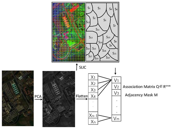
Figure 2.
Superpixel and pixel feature conversion process.
Specifically, an H2 image is divided into superpixels by PCA-SLIC, wherein is the superpixel segmentation scale. Let denote the superpixels set, with as the superpixel, as the number of pixels in , and as the pixel in ( and ).
Since the subsequent output features of the GCN need to be merged with the CNN’s, in order to alleviate the data incompatibility between the two networks, we apply the graphical encoder and decoder proposed in [41] to perform the data structure conversion. It is assumed that the association matrix of conversion is and is denoted as follows [41]:
where denotes the expansion of original data into spatial dimensions and denotes the value at position . Then the matrix of node v in graph () can be expressed as follows [41]:
where is the result of column normalization and represents the process that encodes the pixel map of the HSI into the graph node of G. The superpixel node features are then mapped back to pixel features using the equation as follows [41]:
2.2. Cross-Hop Graph Attention Convolution Module
It is feasible to obtain more node information by the way of stacking multiple convolutional layers in the GCN model; however, this operation will inevitably increase the computational complexity of the network. Merely using a shallow GCN lacks deeper feature information and causes poor classification accuracy. In contrast, the multi-hop graph [46] has more flexibility and can fully utilize the multi-hop node information to broaden the acceptance domain and mine the potential relationship between hop nodes.
As shown in Figure 3, the weight matrix between the superpixel nodes is obtained by the superpixel segmentation algorithm for constructing the neighbor matrix of the multi-hop graph structure; the concrete steps are as follows:
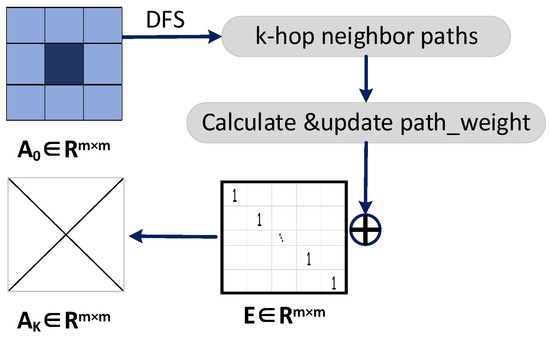
Figure 3.
The procedure for k-hop matrices.
Step 1. Assuming that the graph node is at located at the center, first obtain all the surrounding k-hop neighborhood paths by using a Depth-First Search (DFS) starting at .
Step 2. Calculate the path weights as:
where ,…, represents the nodes in the path. (Note: For the case of having different paths, we select the maximum value of the corresponding path weight and the current weight.)
Step 3. Add the current weight matrix with the unit matrix to ensure that each node is connected to itself to obtain a new k-hop matrix (,,…,).
The k-hop neighbor matrix is applied to find the graph convolution through the GCN and BN layers as follows:
where denotes the output of k-hop neighbor matrix through layer , is the degree matrix of , and indicates weight matrix. The node features of different jumps can feed different visual field information, as in the structure of Figure 4a, through the pyramid feature extraction structure to obtain the features of different depths and splice them to obtain the following:
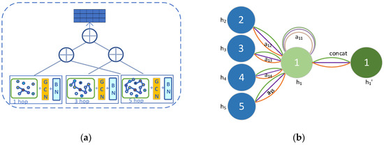
Figure 4.
Cross-hop graph attention module: (a) pyramid structure by cross-connect feature and (b) graph attention mechanism.
To compute the hidden information of each node, as in Figure 4b, a self-attention sharing mechanism was applied to compute the attention coefficients between node and node : . Here, the first-order attention mechanism is carried by merely computing the first-order neighbor nodes of the node , where is a domain of . Then, normalization by the function is executed to make the coefficients more easily comparable across nodes:
Then, the corresponding features undergo a linear combination to calculate the node output features .
To obtain the node features stably, we apply multiple attention mechanisms to obtain multiple sets of new features, which are spliced in feature dimensions and placed into the final fully connected layer to obtain the final features as follows:
where denotes the group of attention coefficients; is the number of heads, which means there are groups of attention coefficients; and denotes splicing operation of the total number of groups in the feature dimensions. denotes the weight matrix, where indicates input feature dimensions and denotes the output feature dimensions, which equal the number of classes of the hyperspectral images.
2.3. CNN-Based Multiscale Feature Extraction Module
Although traditional 2D-CNNs can extract context space features, considering the multi-parameters in the convolutional kernel and a limited number of training samples, we prevent overfitting and enhance training efficiency by applying batch normalization (BN) to each convolutional layer unit [47], which is calculated as follows:
where , , ,, , and denote the size of the convolution kernel and their corresponding indices; indicates the output by the convolutional layer at ; and , , and denote the weight, bias term, and activation function, respectively.
For broadening the sensory field of the network to obtain local features at varied scales, as shown in Figure 5, features are extracted from different sized convolution kernels in parallel, and then the different scale information is integrated by cross-path fusion. Because of the high dimensionality of the HSI spectrum, a 1D convolution kernel is first used in the convolution module to remove redundant spectral information and reduce parameter usage. Then an average pooling layer is used between the different convolutional layers to reduce the feature space size and prevent overfitting, where the pooling window size, stride, and padding size are, respectively, set to 3 × 3, 1, and 1.
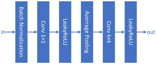
Figure 5.
The structure of ConvBlock.
2.4. Dual-Channel Attention Fusion Module
To better employ the channel relationship between hyperspectral pixels, we utilize the Convolutional Block Attention Network [60] (CBAM) module displayed in Figure 6 to sequentially infer the attention mapping along channel and spatial dimensions independently, multiplying it by the input for adaptive feature refinement.

Figure 6.
Convolutional block attention network module: (a) channel attention module and (b) spatial attention module.
Suppose the input feature map is ; after the CBAM module there are channel and spatial attention maps and and their attention processes is expressed as follows:
Feature fusion inspired by [47] utilizes the cross-attention fusion mechanism as shown in Figure 7.
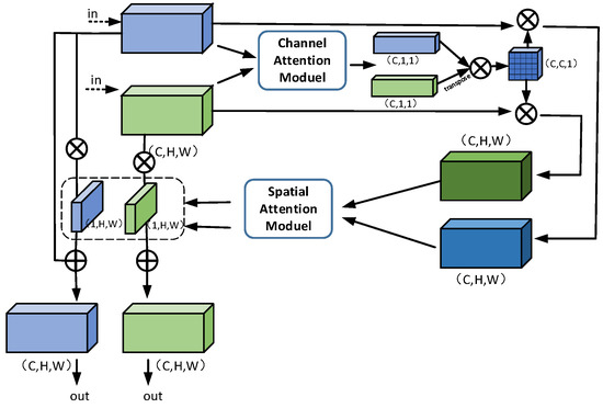
Figure 7.
Dual-channel attention fusion module.
Specifically, the input is first aggregated by global and max pooling on the spatial information of the feature maps to generate two features: and . There is a shared network composed of a multilayer perceptron (MLP) and a hidden layer where the above-mentioned features are input to get a channel attention map :
where and represent the shared weight parameters of the MLP, is the reduction ratio in the hidden layer, and and is the function. From this, we can obtain mappings and , which correspond to the previous two branch features and , respectively, and multiply them to obtain :
After the channel crossing module, the characteristics are obtained as follows:
Unlike the channel attention operation, we input two pooled features into the convolutional layer to generate the spatial attention mapping [47]
where is a convolutional layer with kernel size . Similarly obtain the spatial weight coefficients and , multiply them with the input features, and add the residuals to get the noted features, respectively:
Eventually, through the fully connected layer, the last features are obtained [47] as follows:
where and are the weight and bias. The progress is summarized in Algorithm 1.
| Algorithm 1 Dual-Channel Attention Fusion Algorithm |
| Input: |
| Step 1: Calculate and of separately by global pooling and max pooling. |
| Step 2: Calculate channel weight coefficients for both branches as and according to Equation (12). Step3: Calculate crossover coefficient by Equation (13). Step 4: Use the channel crossover module to calculate and , respectively, according to Equations (14) and (15). Step 5: Similar to steps 1–4 above, calculate the spatial weight coefficients and and the fusion features and by Equations (16)–(18). Step 6: Calculate final fusion features according to Equation (19). |
| Output: |
3. Experimental Details
To validate the effectiveness and generalization of the H2-CHGN, we chose the following three datasets: a classical HSI dataset (Pavia University) and two H2 image datasets (WHU-Hi-LongKou [1] and WHU-Hi-HongHu [61]). They are captured by different sensors for different types of scenes, providing richer samples. This diversity helps to improve the generalization ability of the model so that it performs well in different scenes. Table 1 lists the detailed information about the datasets. Table 2, Table 3 and Table 4 list training and testing set divisions of the three datasets. The comparison methods are SVM (OA: PU = 79.54%, LK = 92.88%, and HH = 66.34%), CEGCN [41] (OA: PU = 97.81%, LK = 98.72%, and HH = 94.01%), SGML (OA: PU = 94.30%, LK = 96.03%, and HH = 92.51%), WFCG (OA: PU = 97.53%, LK = 98.29%, and HH = 93.98%), MSSG-UNet (OA: PU = 98.52%, LK = 98.56%, and HH = 93.73%), MS-RPNet (OA: PU = 96.96%, LK = 97.17%, and HH = 93.56%), AMCGFN (OA: PU = 98.24%, LK = 98.44%, and HH = 94.44%) and H2-CHGN (OA: PU = 99.24%, LK = 99.19%, and HH = 96.60%). To quantitatively and qualitatively assess the classification performance of the network [62], three evaluation indices are used: overall accuracy (OA), average accuracy (AA), and kappa coefficient (Kappa). All experimental results are averaged over ten runs independently. The experiments were run via Python 3.7.16 with i5-8250U CPU and NVIDIA GeForce RTX 3090 GPU.

Table 1.
Information about datasets.

Table 2.
Category information of Pavia University dataset.

Table 3.
Category information of WHU-Hi-LongKou dataset.

Table 4.
Category information of WHU-Hi-HongHu dataset.
3.1. Parametric Setting
Table 5 shows the architecture of the H2-CHGN where it is used for all activation functions. In addition, the network uses the Adam optimizer with a learning rate of 5 ×10⁻⁴ to train. The remaining setup parameters include the superpixel segmentation scale and the number of attentional heads, and the iterations are explained in the following sections. We discuss and analyze these parameters through experiments, and the ultimate optimal parameter settings are shown in Table 6.

Table 5.
The architectural details of H2-CHGN.

Table 6.
Parameter settings for different datasets.
3.2. Analysis of Multi-Head Attention Mechanism in Graph Attention
By using multiple attention heads, a GAT is able to learn the attention weights between different nodes and combine them to obtain a more comprehensive and accurate image features. Notably, the number of heads controls different node relationships that the model is able to learn. Increasing attention heads allows the model to capture richer node relationships and improves the model’s representation, but at the same time this increases the computational complexity and memory overhead and is prone to overfitting. Therefore, as shown in Figure 8, so as to weigh the balance between model performance and computational complexity, the number of heads is taken as 7, 6, and 5 for three datasets individually.

Figure 8.
OAs under a different number of heads and epochs: (a) Pavia University; (b) WHU-Hi-LongKou; and (c) WHU-Hi-HongHu.
3.3. Impact of Superpixel Segmentation Scale
The size of the superpixel segmentation scale molds the size of the graph construction area. The larger the superpixel area, the more pixels are contained in the segmented superpixel area and the fewer the number graph nodes that have to be constructed. The experiments are set ’s as 150, 200, 250, 300, 350, 400. Regions with different numbers of superpixels are visualized in mean color as in Figure 9, where the most representative features of each region can be seen more clearly. The larger the superpixel segmentation scale, the more superpixels in the segmented region, indicating a more detailed segmentation. Figure 10 demonstrates that as the scale increases, the classification accuracy initially increases but eventually declines, with the WHU-Hi-HongHu dataset experiencing a more significant decrease compared to the other two datasets. This is attributed to its greater complexity, featuring 22 categories and a relatively denser distribution of features. When different varieties of the same crop type are planted in a region, finer segmentation can lead to a higher likelihood of misclassifying various pixel categories into a single node. Additionally, the overall accuracy improves again when the segmentation scale increases from 350 to 400, likely due to the enhanced category separability achieved through more detailed segmentation.
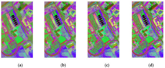
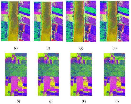
Figure 9.
Mean color visualization of superpixel segmented regions on different datasets: (a–d): Pavia University; (e–h): WHU-Hi-LongKou; and (i–l): WHU-Hi-HongHu.
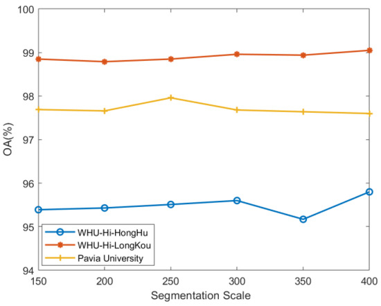
Figure 10.
Effect of different superpixel segmentation scales on classification accuracy.
3.4. Cross-Hopping Connection Analysis
Because HSI contains feature distributions of varying shapes and sizes, the cross-hop mechanism plays a critical role in modeling complex spatial topologies. Precisely, the near-hop graph structure contains fewer nodes, which is good for modeling small feature distributions, but makes it hard to learn continuous smooth features on large one. In contrast to the neighbor-hopping graph structure, in which most of the graph nodes are duplicated, the cross-hopping graph can better model large feature distributions but fails to account for subtle differences. To affirm the competence of the cross-hop hopping operation, we repeated the experiment 10 times for three sets of experiments (123-hop for adjacent hops, 124-hop for cross-even hops, and 135-hop for cross-odd hops). As shown in Figure 11, there is no significant effect for the simpler WHU-Hi-LongKou dataset. In contrast, for other two more complex datasets, the cross odd-hop 135-hop operation has a better performance. The reason can be inferred that the cross-hop mechanism enables a larger range of graph convolution operations, which can effectively extract a wider range of sample information and perform better.
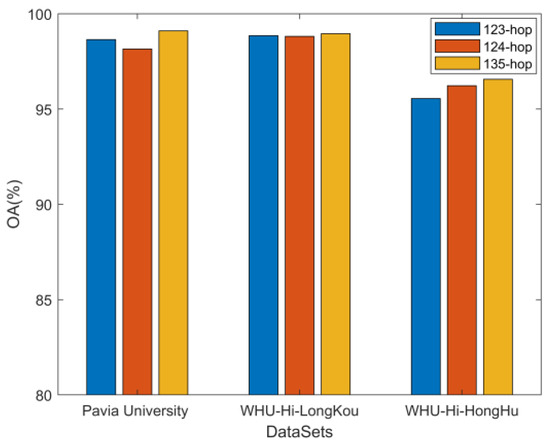
Figure 11.
Effect of different cross-hopping methods on classification accuracy.
4. Comparative Experimental Analysis and Discussions
4.1. Comparison of Classification Performance
The classification accuracies of the diverse methods on the three datasets are described in Table 7, Table 8 and Table 9, and the matching classification diagrams are shown in Figure 12, Figure 13 and Figure 14. From the results, SVM achieves poorer results when the training samples are small. In contrast, GCN-based SGML achieves smoother features, but also suffers from many scattered pretzel noises and susceptibility to misclassification. In addition, other models based on the fusion mechanism of a GCN and a CNN can obviously achieve higher classification accuracy despite their more complex structure, which indicates that the training sample features can be fully exploited by using the superpixel-based multiscale fusion mechanism. As seen in classification Figure 12, Figure 13 and Figure 14, the H2-CHGN achieves better classification results than other models on both classical and double-high (H2) datasets. It is obvious that the model provides a more significant improvement effect on WHU-Hi-HongHu dataset. Its plots vary in size and exhibit a more fragmented distribution, making them susceptible to generating isolated regions of classification errors in classification tasks. The proposed cross-hop graph operation facilitates the acquisition of contextual information and global association features from near to far, achieving a maximum accuracy of 96.6% on the WHU-Hi-HongHu dataset. In summary, the H2-CHGN not only integrates a CNN and a GCN well, but also effectively handles complex spatial features by using superpixel segmentation on the GCN branch, extracts structure-learning multi-scale features by using pyramid features of the spanning-hopping graphs, and captures local and global information by a GAT. The combined effect of superpixel segmentation, cross-hop map convolution, and attention mechanism can alleviate the problem of high spatial-spectral heterogeneity.

Table 7.
Classification accuracy of the Pavia University dataset.

Table 8.
Classification accuracy of the WHU-Hi-LongKou dataset.

Table 9.
Classification accuracy of the WHU-Hi-HongHu dataset.
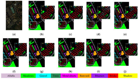
Figure 12.
Classification maps for the Pavia University dataset: (a) False-color image; (b) ground truth; (c) SVM (OA = 79.54%); (d) CEGCN (OA = 97.81%); (e) SGML (OA = 94.30%); (f) WFCG (OA = 97.53%); (g) MSSG-UNet (OA = 98.52%); (h) MS-RPNet (OA = 96.96%); (i) AMGCFN (OA = 98.24%); and (j) H2-CHGN (OA = 99.24%).
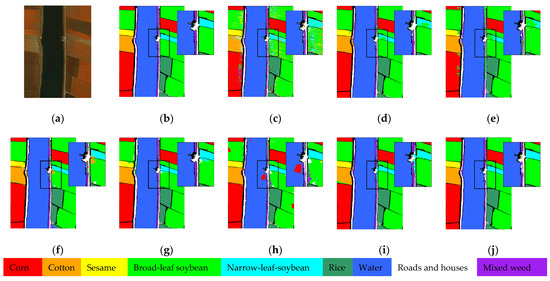
Figure 13.
Classification maps for the WHU-Hi-LongKou dataset: (a) False-color image; (b) ground truth; (c) SVM (OA = 92.88%); (d) CEGCN (OA = 98.72%); (e) SGML (OA = 96.03%); (f) WFCG (OA = 98.29%); (g) MSSG-UNet (OA = 98.56%); (h) MS-RPNet (OA = 97.17%); (i) AMGCFN (OA = 98.44%); and (j) H2-CHGN (OA = 99.19%).
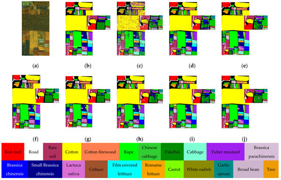
Figure 14.
Classification maps for the WHU-Hi-HongHu dataset: (a) False-color image; (b) Ground truth; (c) SVM (OA = 66.34%); (d) CEGCN (OA = 94.01%); (e) SGML (OA = 92.51%); (f) WFCG (OA = 93.98%); (g) MSSG-UNet (OA = 93.73%); (h) MS-RPNet (OA = 93.56%); (i) AMGCFN (OA = 94.44%); (j) H2-CHGN (OA = 96.60%).
4.2. Ablation Analysis
To validate the efficacy of each module, we conducted ablation experiments on three datasets. Table 10 presents the results of these experiments: (1) and (2) represent the experiments conducted solely on the two-branch module, while (3) and (4) depict the experiments conducted with the combination of the Dual-Channel Fusion module with one or the other of the two branches, respectively. By comparing (1) and (3), as well as (2) and (4), it is evident that the Dual-Channel Fusion module enhances the classification performance by improving the output features of the corresponding branches. Moreover, Experiment (5) demonstrates the indispensable contribution of each component to the overall model.

Table 10.
OA (%) of ablation of each module on three datasets.
4.3. Performance under Limited Samples
H2 data usually have high dimensionality and plenty of spectral bands, but training samples are usually odd in that samples of each category are limited. Therefore, the small-sample learning ability of the model is crucial in HSI classification methods. Experimentally, 0.1–0.6% samples are selected as training samples. As is described in Figure 15, OA increases with more training samples, and the H2-CHGN outperforms the other models on all three datasets. It is worth noting that due to the possible imbalance of samples in hyperspectral datasets, over-sampling of certain categories may lead to a decrease in accuracy with an increase in sampling rate.

Figure 15.
Effect of different numbers of training samples for the methods: (a) Pavia University; (b) WHU-Hi-LongKou; and (c) WHU-Hi-HongHu.
4.4. Visualization by t-SNE
T-distributed stochastic neighbor embedding (t-SNE) [63] is a nonlinear dimensionality reduction technique which is particularly suitable for the visualization of high-dimensional data. Figure 16 shows the t-SNE result of four methods on three datasets. For a more straightforward view, the experiment was visualized by randomly selecting one of the bands of the feature. By comparison, a larger interclass gap and smaller intraclass disparity are displayed in the proposed feature space, and all categories are distinguished by acceptable boundaries [64].
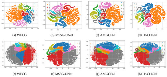

Figure 16.
t-SNE results of different methods on three datasets: (a–d) Pavia University; (e–h) WHU-Hi-LongKou; and (i–l) WHU-Hi-HongHu.
4.5. Comparison of Running Time
To evaluate the efficiency of the H2-CHGN, the running times of different methods were recorded on the same computing platform, and comparisons are shown in Table 11. In this paper, the H2-CHGN, as in CEGCNs and MSSGU-Nets, inputs the whole H2 image into the network and classifies all the pixels in parallel through two branches, which also results in a shorter training time of the network compared to other methods and proves the superiority of the method.

Table 11.
Running time for different methods.
5. Conclusions
In this paper, a cross-hop graph network (H2-CHGN) model for H2 image classification is proposed to alleviate the spatial heterogeneity and spectral variability of an H2 image. It is also essentially a hybrid neural network based on a superpixel-based GCN and a pixel-based CNN to extract spatial and global spectral features. Among them, a cross-hop graph attention network (CGAT) branch widens the range of graph convolution and the pyramid feature extraction structure is utilized to fuse multilevel features. So as to better capture relationship between nodes and contextual information, the H2-CHGN also employs a graph attention mechanism that specializes in graph-structured data. Meanwhile, the multi-scale convolutional neural network (MCNN) employs dual convolutional kernels to extract features at different scales and obtains multi-scale localized features in pixel level by means of cross connectivity. Finally, the dual-channel attention fusion module is used to effectively integrate multi-scale information, while strengthening the key features and improving generalization capability. Experimental results verify the validity and generalization of the H2-CHGN. Specifically, the overall accuracy of the three datasets (Pavia University, WHU-Hi-LongKou, WHU-Hi-HongHu) is as high as 99.24%, 99.19%, 96.60% respectively.
Our study possesses certain limitations containing a large number of model parameters and high computational demands. First, we noticed that the H2-CHGN is the result of superpixel segmentation, cross-hop convolution, and the attention mechanism working together. Therefore, suitable parameter matching is essential. In addition, a GCN needs to construct the adjacency matrix on all data, while the H2-CHGN can reduce the computational cost by cross-hop graph convolution.
In the future, we will explore strategies to enhance the cross-hop graph by employing more advanced techniques, such as transformers. Additionally, we aim to develop lighter-weight networks to reduce complexity while preserving performance.
Author Contributions
Conceptualization, T.W. and H.C.; methodology, T.W. and B.Z.; software T.C.; validation, W.D.; resources, H.C.; data curation, T.W.; writing—original draft preparation, T.W. and H.C.; writing—review and editing, T.C. and W.D.; visualization, T.W.; supervision, B.Z.; project administration, T.C.; funding acquisition, H.C. All authors have read and agreed to the published version of the manuscript.
Funding
This work was supported in part by the National Natural Science Foundation of China (62176217), the Innovation TeamFunds of ChinaWest Normal University (KCXTD2022-3), the Sichuan Science and Technology Program of China (2023YFG0028, 2023YFS0431), the A Ba Achievements Transformation Program (R23CGZH0001), the Sichuan Science and Technology Program of China (2023ZYD0148, 2023YFG0130), and Sichuan Province Transfer Payment Application and Development Program (R22ZYZF0004).
Data Availability Statement
Dataset available on request from the authors.
Conflicts of Interest
The authors declare no conflicts of interest.
References
- Zhong, Y.; Hu, X.; Luo, C.; Wang, X.; Zhao, J.; Zhang, L. WHU-Hi: UAV-borne hyperspectral with high spatial resolution (H2) benchmark datasets and classifier for precise crop identification based on deep convolutional neural network with CRF. Remote Sens. Environ. 2020, 250, 112012. [Google Scholar] [CrossRef]
- Paoletti, M.E.; Haut, J.M.; Plaza, J.; Plaza, A. Deep learning classifiers for hyperspectral imaging: A review. ISPRS J. Photogramm. Remote Sens. 2019, 158, 279–317. [Google Scholar] [CrossRef]
- Hong, D.; Gao, L.; Yao, J.; Zhang, B.; Plaza, A.; Chanussot, J. Graph convolutional networks for hyperspectral image classification. IEEE Trans. Geosci. Remote Sens. 2020, 59, 5966–5978. [Google Scholar] [CrossRef]
- Landgrebe, D. Hyperspectral image data analysis. IEEE Signal Process. Mag. 2002, 19, 17–28. [Google Scholar] [CrossRef]
- Shimoni, M.; Haelterman, R.; Perneel, C. Hypersectral imaging for military and security applications: Combining myriad processing and sensing techniques. IEEE Geosci. Remote Sens. Mag. 2019, 7, 101–117. [Google Scholar] [CrossRef]
- Li, S.; Song, W.; Fang, L.; Chen, Y.; Ghamisi, P.; Benediktsson, J.A. Deep learning for hyperspectral image classification: An overview. IEEE Trans. Geosci. Remote Sens. 2019, 57, 6690–6709. [Google Scholar] [CrossRef]
- Long, H.; Chen, T.; Chen, H.; Zhou, X.; Deng, W. Principal space approximation ensemble discriminative marginalized least-squares regression for hyperspectral image classification. Eng. Appl. Artif. Intell. 2024, 133, 108031. [Google Scholar] [CrossRef]
- Li, J.; Zheng, K.; Yao, J.; Gao, L.; Hong, D. Deep unsupervised blind hyperspectral and multispectral data fusion. IEEE Geosci. Remote Sens. Lett. 2022, 19, 1–5. [Google Scholar] [CrossRef]
- Chen, H.; Long, H.; Chen, T.; Song, Y.; Chen, H.; Zhou, X.; Deng, W. M3FuNet: An Unsupervised Multivariate Feature Fusion Network for Hyperspectral Image Classification. IEEE Trans. Geosci. Remote Sens. 2024, 62, 1–15. [Google Scholar]
- Makantasis, K.; Karantzalos, K.; Doulamis, A.; Doulamis, N. Deep supervised learning for hyperspectral data classification through convolutional neural networks. In Proceedings of the 2015 IEEE international geoscience and remote sensing symposium (IGARSS), Milan, Italy, 26–31 July 2015; pp. 4959–4962. [Google Scholar]
- Zhong, Z.; Li, J.; Luo, Z.; Chapman, M. Spectral–spatial residual network for hyperspectral image classification: A 3-D deep learning framework. IEEE Trans. Geosci. Remote Sens. 2017, 56, 847–858. [Google Scholar] [CrossRef]
- Roy, S.K.; Krishna, G.; Dubey, S.R.; Chaudhuri, B.B. HybridSN: Exploring 3-D–2-D CNN feature hierarchy for hyperspectral image classification. IEEE Geosci. Remote Sens. Lett. 2019, 17, 277–281. [Google Scholar] [CrossRef]
- Chen, H.; Ru, J.; Long, H.; He, J.; Chen, T.; Deng, W. Semi-supervised adaptive pseudo-label feature learning for hyperspectral image classification in internet of things. IEEE Internet Things J. 2024. [Google Scholar] [CrossRef]
- Vaswani, A. Attention is all you need. arXiv 2017, arXiv:1706.03762. [Google Scholar]
- Hong, D.; Han, Z.; Yao, J.; Gao, L.; Zhang, B.; Plaza, A.; Chanussot, J. SpectralFormer: Rethinking hyperspectral image classification with transformers. IEEE Trans. Geosci. Remote Sens. 2021, 60, 1–15. [Google Scholar] [CrossRef]
- Dosovitskiy, A.; Beyer, L.; Kolesnikov, A.; Weissenborn, D.; Zhai, X.; Unterthiner, T.; Dehghani, M.; Minderer, M.; Heigold, G.; Gelly, S.; et al. An image is worth 16 × 16 words: Transformers for image recognition at scale. arXiv 2020, arXiv:2010.11929. [Google Scholar]
- Sun, L.; Zhang, H.; Zheng, Y.; Wu, Z.; Ye, Z.; Zhao, H. MASSFormer: Memory-Augmented Spectral-Spatial Transformer for Hyperspectral Image Classification. IEEE Trans. Geosci. Remote Sens. 2024, 62, 5516415. [Google Scholar] [CrossRef]
- Johnson, F.; Adebukola, O.; Ojo, O.; Alaba, A.; Victor, O. A task performance and fitness predictive model based on neuro-fuzzy modeling. Artif. Intell. Appl. 2024, 2, 66–72. [Google Scholar] [CrossRef]
- Zhao, H.; Gao, Y.; Deng, W. Defect detection using shuffle Net-CA-SSD lightweight network for turbine blades in IoT. IEEE Internet Things J. 2024. [Google Scholar] [CrossRef]
- Li, W.; Liu, D.; Li, Y.; Hou, M.; Liu, J.; Zhao, Z.; Guo, A.; Zhao, H.; Deng, W. Fault diagnosis using variational autoencoder GAN and focal loss CNN under unbalanced data. Struct. Health Monit. 2024. [Google Scholar] [CrossRef]
- Yu, C.; Zhao, X.; Gong, B.; Hu, Y.; Song, M.; Yu, H.; Chang, C.I. Distillation-Constrained Prototype Representation Network for Hyperspectral Image Incremental Classification. IEEE Trans. Geosci. Remote Sens. 2024, 62, 5507414. [Google Scholar] [CrossRef]
- Bhosle, K.; Musande, V. Evaluation of deep learning, C.N.N Model for recognition of Devanagari digit. Artif. Intell. Appl. 2023, 1, 114–118. [Google Scholar]
- Sun, Q.; Chen, J.; Zhou, L.; Ding, S.; Han, S. A study on ice resistance prediction based on deep learning data generation method. Ocean. Eng. 2024, 301, 117467. [Google Scholar] [CrossRef]
- Wang, Z.; Xu, N.; Bao, X.; Wu, J.; Cui, X. Spatio-temporal deep learning model for accurate streamflow prediction with multi-source data fusion. Environ. Model. Softw. 2024, 178, 106091. [Google Scholar] [CrossRef]
- Shao, H.; Zhou, X.; Lin, J.; Liu, B. Few-shot cross-domain fault diagnosis of bearing driven by Task-supervised ANIL. IEEE Internet Things J. 2024, 11, 22892–22902. [Google Scholar] [CrossRef]
- Dong, J.; Wang, Z.; Wu, J.; Cui, X.; Pei, R. A novel runoff prediction model based on support vector machine and gate recurrent unit with secondary mode decomposition. Water Resour. Manag. 2024, 38, 1655–1674. [Google Scholar] [CrossRef]
- Preethi, P.; Mamatha, H.R. Region-based convolutional neural network for segmenting text in epigraphical images. Artif. Intell. Appl. 2023, 1, 119–127. [Google Scholar] [CrossRef]
- Zhao, H.; Wu, Y.; Deng, W. An interpretable dynamic inference system based on fuzzy broad learning. IEEE Trans. Instrum. Meas. 2023, 72, 2527412. [Google Scholar] [CrossRef]
- Yan, S.; Shao, H.; Wang, J.; Zheng, X.; Liu, B. LiConvFormer: A lightweight fault diagnosis framework using separable multiscale convolution and broadcast self-attention. Expert Syst. Appl. 2024, 237, 121338. [Google Scholar] [CrossRef]
- Wang, Z.; Wang, Q.; Liu, Z.; Wu, T. A deep learning interpretable model for river dissolved oxygen multi-step and interval prediction based on multi-source data fusion. J. Hydrol. 2024, 629, 130637. [Google Scholar] [CrossRef]
- Li, T.Y.; Shu, X.Y.; Wu, J.; Zheng, Q.X.; Lv, X.; Xu, J.X. Adaptive weighted ensemble clustering via kernel learning and local information preservation. Knowl.-Based Syst. 2024, 294, 111793. [Google Scholar] [CrossRef]
- Li, M.; Lv, Z.; Cao, Q.; Gao, J.; Hu, B. Automatic assessment method and device for depression symptom severity based on emotional facial expression and pupil-wave. IEEE Trans. Instrum. Meas. 2024. [Google Scholar]
- Li, X.; Zhao, H.; Deng, W. IOFL: Intelligent-optimization-based federated learning for Non-IID data. IEEE Internet Things J. 2024, 11, 16693–16699. [Google Scholar] [CrossRef]
- Xu, J.; Li, T.; Zhang, D.; Wu, J. Ensemble clustering via fusing global and local structure information. Expert Syst. Appl. 2024, 237, 121557. [Google Scholar] [CrossRef]
- Li, M.; Wang, Y.Q.; Yang, C.; Lu, Z.; Chen, J. Automatic diagnosis of depression based on facial expression information and deep convolutional neural network. IEEE Trans. Comput. Soc. Syst. 2024. [Google Scholar] [CrossRef]
- Veličković, P.; Cucurull, G.; Casanova, A.; Romero, A.; Lio, P.; Bengio, Y. Graph attention networks. arXiv 2017, arXiv:1710.10903. [Google Scholar]
- Saber, S.; Amin, K.; Pławiak, P.; Tadeusiewicz, R.; Hammad, M. Graph convolutional network with triplet attention learning for person re-identification. Inf. Sci. 2022, 617, 331–345. [Google Scholar] [CrossRef]
- Sellars, P.; Aviles-Rivero, A.I.; Schönlieb, C.B. Superpixel contracted graph-based learning for hyperspectral image classification. IEEE Trans. Geosci. Remote Sens. 2020, 58, 4180–4193. [Google Scholar] [CrossRef]
- Wan, S.; Gong, C.; Zhong, P.; Du, B.; Zhang, L.; Yang, J. Multiscale dynamic graph convolutional network for hyperspectral image classification. IEEE Trans. Geosci. Remote Sens. 2019, 58, 3162–3177. [Google Scholar] [CrossRef]
- Li, Y.; Xi, B.; Li, J.; Song, R.; Xiao, Y.; Chanussot, J. SGML: A symmetric graph metric learning framework for efficient hyperspectral image classification. IEEE J. Sel. Top. Appl. Earth Obs. Remote Sens. 2021, 15, 609–622. [Google Scholar] [CrossRef]
- Liu, Q.; Xiao, L.; Yang, J.; Wei, Z. CNN-enhanced graph convolutional network with pixel-and superpixel-level feature fusion for hyperspectral image classification. IEEE Trans. Geosci. Remote Sens. 2020, 59, 8657–8671. [Google Scholar] [CrossRef]
- Liu, Q.; Xiao, L.; Yang, J.; Wei, Z. Multilevel superpixel structured graph U-Nets for hyperspectral image classification. IEEE Trans. Geosci. Remote Sens. 2021, 60, 1–5. [Google Scholar] [CrossRef]
- Dong, Y.; Liu, Q.; Du, B.; Zhang, L. Weighted feature fusion of convolutional neural network and graph attention network for hyperspectral image classification. IEEE Trans. Image Process. 2022, 31, 1559–1572. [Google Scholar] [CrossRef]
- Ding, Y.; Zhang, Z.; Zhao, X.; Hong, D.; Cai, W.; Yang, N.; Wang, B. Multi-scale receptive fields: Graph attention neural network for hyperspectral image classification. Expert Syst. Appl. 2023, 223, 119858. [Google Scholar] [CrossRef]
- Ding, Y.; Zhang, Z.; Zhao, X.; Hong, D.; Cai, W.; Yu, C.; Yang, N.; Cai, W. Multi-feature fusion: Graph neural network and CNN combining for hyperspectral image classification. Neurocomputing 2022, 501, 246–257. [Google Scholar] [CrossRef]
- Xue, H.; Sun, X.K.; Sun, W.X. Multi-hop hierarchical graph neural networks. In Proceedings of the 2020 IEEE International Conference on Big Data and Smart Computing (BigComp), Busan, Republic of Korea, 19–22 February 2020; IEEE: Piscataway, NJ, USA, 2020; pp. 82–89. [Google Scholar]
- Zhou, H.; Luo, F.; Zhuang, H.; Weng, Z.; Gong, X.; Lin, Z. Attention multi-hop graph and multi-scale convolutional fusion network for hyperspectral image classification. IEEE Trans. Geosci. Remote Sens. 2023, 61, 1–14. [Google Scholar]
- Xiao, Y.; Shao, H.; Lin, J.; Huo, Z.; Liu, B. BCE-FL: A secure and privacy-preserving federated learning system for device fault diagnosis under Non-IID Condition in IIoT. IEEE Internet Things J. 2024, 11, 14241–14252. [Google Scholar] [CrossRef]
- Tao, S.; Wang, K.; Jin, T.; Wu, Z.; Lei, Z.; Gao, S. Spherical search algorithm with memory-guided population stage-wise control for bound-constrained global optimization problems. Appl. Soft Comput. 2024, 161, 111677. [Google Scholar] [CrossRef]
- Song, Y.J.; Han, L.H.; Zhang, B.; Deng, W. A dual-time dual-population multi-objective evolutionary algorithm with application to the portfolio optimization problem. Eng. Appl. Artiffcial Intell. 2024, 133, 108638. [Google Scholar] [CrossRef]
- Li, F.; Chen, J.; Zhou, L.; Kujala, P. Investigation of ice wedge bearing capacity based on an anisotropic beam analogy. Ocean Eng. 2024, 302, 117611. [Google Scholar] [CrossRef]
- Chen, H.; Heidari, A.A.; Chen, H.; Wang, M.; Pan, Z.; Gandomi, A.H. Multi-population differential evolution-assisted Harris hawks optimization: Framework and case studies. Future Gener. Comput. Syst. 2020, 111, 175–198. [Google Scholar] [CrossRef]
- Zhao, H.; Wang, L.; Zhao, Z.; Deng, W. A new fault diagnosis approach using parameterized time-reassigned multisynchrosqueezing transform for rolling bearings. IEEE Trans. Reliab. 2024. [Google Scholar] [CrossRef]
- Xie, P.; Deng, L.; Ma, Y.; Deng, W. EV-Call 120: A new-generation emergency medical service system in China. J. Transl. Intern. Med. 2024, 12, 209–212. [Google Scholar] [CrossRef] [PubMed]
- Ahmadianfar, I.; Heidari, A.A.; Gandomi, A.H.; Chu, X.; Chen, H. RUN Beyond the Metaphor: An Efficient Optimization Algorithm Based on Runge Kutta Method. Expert Syst. Appl. 2021, 115079. [Google Scholar] [CrossRef]
- Deng, W.; Chen, X.; Li, X.; Zhao, H. Adaptive federated learning with negative inner product aggregation. IEEE Internet Things J. 2023, 11, 6570–6581. [Google Scholar] [CrossRef]
- Gao, J.; Wang, Z.; Jin, T.; Cheng, J.; Lei, Z.; Gao, S. Information gain ratio-based subfeature grouping empowers particle swarm optimization for feature selection. Knowl.-Based Syst. 2024, 286, 111380. [Google Scholar] [CrossRef]
- Yang, Y.; Chen, H.; Heidari, A.A.; Gandomi, A.H. Hunger games search: Visions, conception, implementation, deep analysis, perspectives, and towards performance shifts. Expert Syst. Appl. 2021, 177, 114864. [Google Scholar] [CrossRef]
- Wang, J.; Shao, H.; Peng, Y.; Liu, B. PSparseFormer: Enhancing fault feature extraction based on parallel sparse self-attention and multiscale broadcast feed-forward block. IEEE Internet Things J. 2024, 11, 22982–22991. [Google Scholar] [CrossRef]
- Woo, S.; Park, J.; Lee, J.Y.; Kweon, I.S. Cbam: Convolutional block attention module. In Proceedings of the European conference on computer vision (ECCV), Munich, Gernamy, 8–14 September 2018; pp. 3–19. [Google Scholar]
- Zhong, Y.; Wang, X.; Xu, Y.; Wang, S.; Jia, T.; Hu, X.; Zhao, J.; Wei, L.; Zhang, L. Mini-UAV-borne hyperspectral remote sensing: From observation and processing to applications. IEEE Geosci. Remote Sens. Mag. 2018, 6, 46–62. [Google Scholar] [CrossRef]
- Chen, H.; Wang, T.; Chen, T.; Deng, W. Hyperspectral image classification based on fusing S3-PCA, 2D-SSA and random patch network. Remote Sens. 2023, 15, 3402. [Google Scholar] [CrossRef]
- Van der Maaten, L.; Hinton, G. Visualizing data using t-SNE. J. Mach. Learn. Res. 2008, 9, 2579–2605. [Google Scholar]
- Yang, J.; Du, B.; Wang, D.; Zhang, L. ITER: Image-to-pixel representation for weakly supervised HSI classification. IEEE Trans. Image Process. 2024, 33, 257–272. [Google Scholar] [CrossRef] [PubMed]
Disclaimer/Publisher’s Note: The statements, opinions and data contained in all publications are solely those of the individual author(s) and contributor(s) and not of MDPI and/or the editor(s). MDPI and/or the editor(s) disclaim responsibility for any injury to people or property resulting from any ideas, methods, instructions or products referred to in the content. |
© 2024 by the authors. Licensee MDPI, Basel, Switzerland. This article is an open access article distributed under the terms and conditions of the Creative Commons Attribution (CC BY) license (https://creativecommons.org/licenses/by/4.0/).