Spatial Feature Enhancement and Attention-Guided Bidirectional Sequential Spectral Feature Extraction for Hyperspectral Image Classification

Abstract

Hyperspectral images have the characteristics of high spectral resolution and low spatial resolution, which will make the extracted features insufficient and lack detailed information about ground objects, thus affecting the accuracy of classification. The numerous spectral bands of hyperspectral images contain rich spectral features but also bring issues of noise and redundancy. To improve the spatial resolution and fully extract spatial and spectral features, this article proposes an improved feature enhancement and extraction model (IFEE) using spatial feature enhancement and attention-guided bidirectional sequential spectral feature extraction for hyperspectral image classification. The adaptive guided filtering is introduced to highlight details and edge features in hyperspectral images. Then, an image enhancement module composed of two-dimensional convolutional neural networks is used to improve the resolution of the image after adaptive guidance filtering and provide a high-resolution image with key features emphasized for the subsequent feature extraction module. The proposed spectral attention mechanism helps to extract more representative spectral features, emphasizing useful information while suppressing the interference of noise. Experimental results show that our method outperforms other comparative methods even with very few training samples.

1. Introduction

In the field of remote sensing imaging earlier, the electromagnetic wave reflection of objects was often used to obtain the feature information of objects, which could obtain good imaging results for distant targets. However, the information obtained from electromagnetic waves was mainly two-dimensional (2D) spatial information, and there were still some limitations in detecting and classifying objects being observed. In the 1960s, the concept of hyperspectral remote sensing began to emerge. Compared with remote sensing imaging, hyperspectral remote sensing can obtain spectral information in addition to spatial information. The spectral information and spatial information mentioned here are one-dimensional and two-dimensional, respectively, so the original hyperspectral image (HSI) [1] containing these two kinds of information is a three-dimensional data cube with multiple bands. Spectral information contains detailed descriptions of ground objects, including small differences between different categories, and has a better effect on feature recognition, which also makes hyperspectral images widely used in the collaborative classification of multi-source data in the field of remote sensing. In addition, the large amount of information and high spectral resolution of hyperspectral images also make them play an increasingly important role in scenarios such as forest fire prevention, ocean exploration, environment detection [2], and disaster assessment, and become the hotspots of research.

Hyperspectral image classification is a common research direction in the field of HSI processing, which uses a large number of continuous narrow spectral band features and spatial features acquired during hyperspectral imaging to determine the category of each pixel. The earliest HSI classification method only extracted the spectral information of images as the basis for feature classification, such as the support vector machine (SVM) proposed by Melgani and Bruzzone [3]. SVM converts input images into points in space by using the labeling information in the training dataset, and effectively separates samples of different categories in space by searching for the best hyperplane, thus achieving efficient classification. However, SVM is limited by the low spatial resolution of HSIs and the sensitivity to parameter selection. In 1933, the principal component analysis (PCA) method was proposed [4]. Camps et al. [5] initially used a hybrid kernel function to combine spectral and spatial features, which required complex calculations, so Tarabalka et al. [6] proposed the method of clustering and watershed segmentation in 2010 to improve the extraction of spatial features and simplify the calculation process. However, there may be certain information loss in PCA as well as the disability of retaining the nonlinear correlation between samples, which often leads to the lack of sufficient feature information for classification.

Among the methods that focus on spatial feature processing, guided filtering has gradually gained people’s attention in recent years because of its ability to better optimize the results of morphological filtering. Guided filtering constructs a local linear model of the guidance image and the output image, solving the difference function between input and output for implicit filtering, and the edge information of the guidance image is extracted and emphasized. He et al. [7] first proposed a guided filtering method and applied it to spatial feature extraction, whereas Li et al. [8] added an edge-preserving filter and got better classification results. In 2019, Guo et al. [9] proposed multi-scale spatial features and cross-domain convolutional neural networks (MSCNN) to combine guided filtering with deep learning for spatial feature extraction. The multi-scale spatial features obtained by guided filtering were reordered for classification, which greatly improved the classification accuracy. But there was often detailed information lost in traditional guided filtering, and the extraction of edge information was insufficient, influencing the accuracy of classification results.

With the help of deep learning (DL), feature extraction is greatly improved in HSI classification, where a convolutional neural network (CNN) is widely used. Zhao et al. [10] added dimensionality reduction to the two-dimensional convolutional neural network (2DCNN) to obtain deeper spatial and spectral features for better classification results. Subsequently, the three-dimensional convolutional neural network (3DCNN) [11], which outperformed 2DCNN, was proposed. 3DCNN divided the HSI into many neighborhood blocks as the input of the network, and fully extracted the spatial spectral features to improve the classification effects, which took huge amount of calculation and training samples in the case of limited labeled samples. In 2017, Mou et al. [12] proposed to use time series networks that were relatively simple and with less computational cost for HSI classification, including the long short-term memory (LSTM) network. To make better use of spectral features for classification, spectral attention mechanism was proposed. Squeeze and excitation net (SENet) [13] squeezed each channel through a pooling operation and learned attention weights between channels with an activation function. Efficient channel attention (ECA) [14] uses one-dimensional convolution to learn attention weights. And the idea of the convolutional block attention module (CBAM) [15] was to combine traditional channel attention and spatial attention.

The end-to-end spectral-spatial residual network (SSRN) proposed by Zhong et al. [16] implemented the residual module to extract continuous spatial and spectral features of HSI, respectively, and achieved classification with fused spatial and spectral features. The flaw of SSRN was that only single-scale features were considered, and the extraction of global features was not sufficient. Song et al. [17] proposed the deep feature fusion network (DFFN), which used residual learning to synthesize the outputs of different layers of the network but lost some spatial features and lacked contextual information. Based on the residual block, Mu et al. [18] constructed 3D-2D alternating residual blocks for further extraction of multi-scale spatial and spectral features. Both the hybrid spectral convolutional neural network (HybridSN) [19] and the spectral-spatial feature tokenization transformer (SSFTT) [20] proposed recently adopted the residual block structure that combined 2DCNN and 3DCNN for joint features extraction, while SSFTT added a transformer module to represent high-level semantic features. However, SSFTT did not fully consider the details and edge information of HSIs. In 2021, the HSI spectral-spatial classification method based on deep adaptive feature fusion (SSDF) [21] was proposed with a U-shaped, network-based module for feature fusion. Although it greatly combined multi-scale features for better classification results, the generalization of feature fusion operations still needed to be strengthened.

In recent years, many HSI classifiers have introduced Transformers [22] and self-attention modules since Vision Transformer (ViT) [23] was proposed in 2021. He et al. [24] first applied the Transformer model to HSI classification and achieved good results. Hong et al. [25] focused on improving spectral feature extraction in Transformer, proposing Spectralformer to learn spectral sequence information between neighbor channels. Combining Transformer with deep learning was also a good idea to make full use of two different models [26]. Yang et al. [27] changed the structure of Transformer and took the convolution process as embedding. Interactive spectral-spatial transformer (ISSFormer) [28] combined the multi-head self-attention mechanism (MHSA) for spectral features with the local spatial perception mechanism (LSP) for spatial features and had a feature interaction mechanism. To fully explore the rich semantic information in HSIs, SemanticFormer [29] was proposed to learn discriminative visual representations using semantic tokens.

So far, there are still some intractable problems with existing DL-based methods. The low spatial resolution of HSIs often leads to fewer details of ground objects, so it is generally difficult to obtain rich and detailed spatial features, which limits the final classification performance. How to improve the spatial resolution of HSIs and enhance spatial features in HSIs for better classification performance is still a problem to be solved. What’s more, HSIs have dozens to hundreds of continuous bands containing abundant spectral information. By extracting spectral features and capturing the subtle spectral differences between different bands, the accuracy of classification can be further improved. However, the strong correlation between spectral bands and the number of bands makes the extraction of spectral features prone to the influence of noise and information redundancy, and the dimensionality reduction of HSIs may ignore boundary information, which is not conducive to good classification results. In addition, there is always a small number of hyperspectral samples available for training, and labeling requires time and effort, but a good effect of DL demands massive training data. Due to this contradiction, it is necessary to find a model that can get good classification performances with fewer training samples.

To address the problems above, this paper proposes an improved feature enhancement and extraction model (IFEE) using spatial feature enhancement and attention-guided bidirectional sequential spectral feature extraction for hyperspectral image classification. Through adaptive guided filtering, the subtle features and edge information of the input image are preserved and enhanced in the filtered image, which helps to make the categories more distinguishable. With the introduction of a spatial feature enhancement module composed of 2DCNNs, IFEE can improve the resolution of the image after adaptive guidance filtering and provide a high-resolution image with key features emphasized for the subsequent feature extraction module, which will significantly enhance the effect of spatial feature extraction and effectively improve the classification performance. In addition, we refer to the multi-scale and multi-level feature extraction (MMFE) module proposed in SSDF for spatial features extraction to combine deep and shallow convolution features, which adds 2D convolution with different kernels after each pooling layer to get multi-level spatial features. Considering the effect of noise and information redundancy on spectral features extraction, the spectral attention mechanism combined with bidirectional sequential spectral features extraction is designed to emphasize significant and representative spectral features and suppress noise interference, which reduces the interference and increases the classification accuracy. We also discuss the performance of the proposed IFEE with fewer training samples. The main contributions of this paper can be concluded as follows:

(1)

As the effect of traditional guided filtering is limited with fixed regularization coefficients, we introduce an adaptive guided filtering module to preserve and enhance the subtle features and edge information of the input HSIs, which may be lost in dimensionality reduction operations.

(2)

The low spatial resolution of HSIs makes it hard to obtain sufficient spatial features and details of ground objects, thus limiting the classification performance. As a response, we propose a lightweight image enhancement module composed of 2DCNNs to improve the spatial resolution of the feature map after adaptive guided filtering processing and enhance spatial features, preparing more detailed spatial information for feature extraction.

(3)

To reduce the noise and mitigate the impact of data redundancy in spectral dimension, we design a spectral attention mechanism creatively taking spatial patches and sequences randomly selected from original HSIs as two different inputs, which can emphasize representative spectral channels as well as suppressing noise. The spectral attention mechanism is combined with bidirectional sequential spectral features extraction, which further improves the classification accuracy.

(4)

In consideration of the situation that labeled samples are limited in reality, we have discussed the classification performance of the proposed IFEE with a small number of training samples. Our method can get the best classification results on three datasets with only five labeled samples per class for training.

2. Materials and Methods

2.1. Guided Filtering

Traditional guided filtering [30] better preserves the edge gradient information of the original image by introducing the original image as the guidance image, supplementing the image information lost by filtering to a certain extent. There is a local linear relationship between the input and output of guided filtering, which only exists in the square local window θ_k with the size of (2r + 1) × (2r + 1). r is a parameter controlling the size of the window, and k indicates the center pixel of the window. Suppose the filtered image is ff and the input guidance image is I; then the i-th channel feature map of the filtered image ff_i is

$$f{f}_i=a_k{I}_i+d_k\hspace{1em}\hspace{1em}\hspace{1em}\forall i\in {\theta }_k,f{f}_i\in ff$$

(1)

where a_k and d_k are unknown coefficients that will be solved by minimizing the cost function between the input image s and output image ff. The cost function E and the expressions to obtain coefficients are defined as

$$E\left(a_k,d_k\right)={\displaystyle \sum _{i\in {\omega }_k}\left({\left(a_k{I}_i+d_k-s_i\right)}^2+\lambda {{\mathrm{a}}_k}^2\right)}$$

(2)

$$a_k={\displaystyle \frac{1}{\left|\theta \right|}}{\displaystyle \frac{{\displaystyle \sum _{i\in {\theta }_k}{I}_i{s}_i-{\mu }_k{\overline{s}}_k}}{{\sigma }_k^2+\lambda }}$$

(3)

$$d_k=s_k-a_k{\mu }_k$$

(4)

$\lambda$ in Equation (2) is a regularization parameter that is used to control the value of the parameter a_k, and is usually a given value. The value of coefficients is determined by μ_k, the mean of the guidance image I, as well as the variance ${\sigma }_k^2$. The mean of the input image is expressed as ${\overline{s}}_k$, and $\left|\theta \right|$ in Equation (3) indicates how many pixels are contained in the window θ_k. From the linear relationship between the guided filtering output and guidance image, it can be concluded that $\Delta f{f}_i=a_k\Delta I_i$, so the edge gradient information in the guidance image will be retained by the output image, as well as supplementing certain information of image features.

2.2. Image Enhancement and 2D Convolution

The traditional image enhancement methods are the spatial domain method for computing pixel gray values [31], the frequency domain method for transforming spectral components [32], and the combination of these two methods [33]. Common methods including histogram equalization and wavelet transform [34] are characterized by simplicity and speed, but ignore the context. The introduction of CNN greatly improves the effect of image enhancement. The mapping relationship between the original image and the high-spatial-resolution image is learned through the CNN structure, which can enhance a certain part of the image information. Specifically, CNN structure first utilizes convolutional layers to extract features from the input image. During the convolution process, the network learns local features in the image, such as edges and textures. As the depth of the network increases, the level of abstraction of features also increases gradually, with more complex image structures to be represented. The subsequently extracted low-resolution image features are mapped into the space of the high-resolution image by up-sampling or decoder to gradually recover the details and structure of the image.

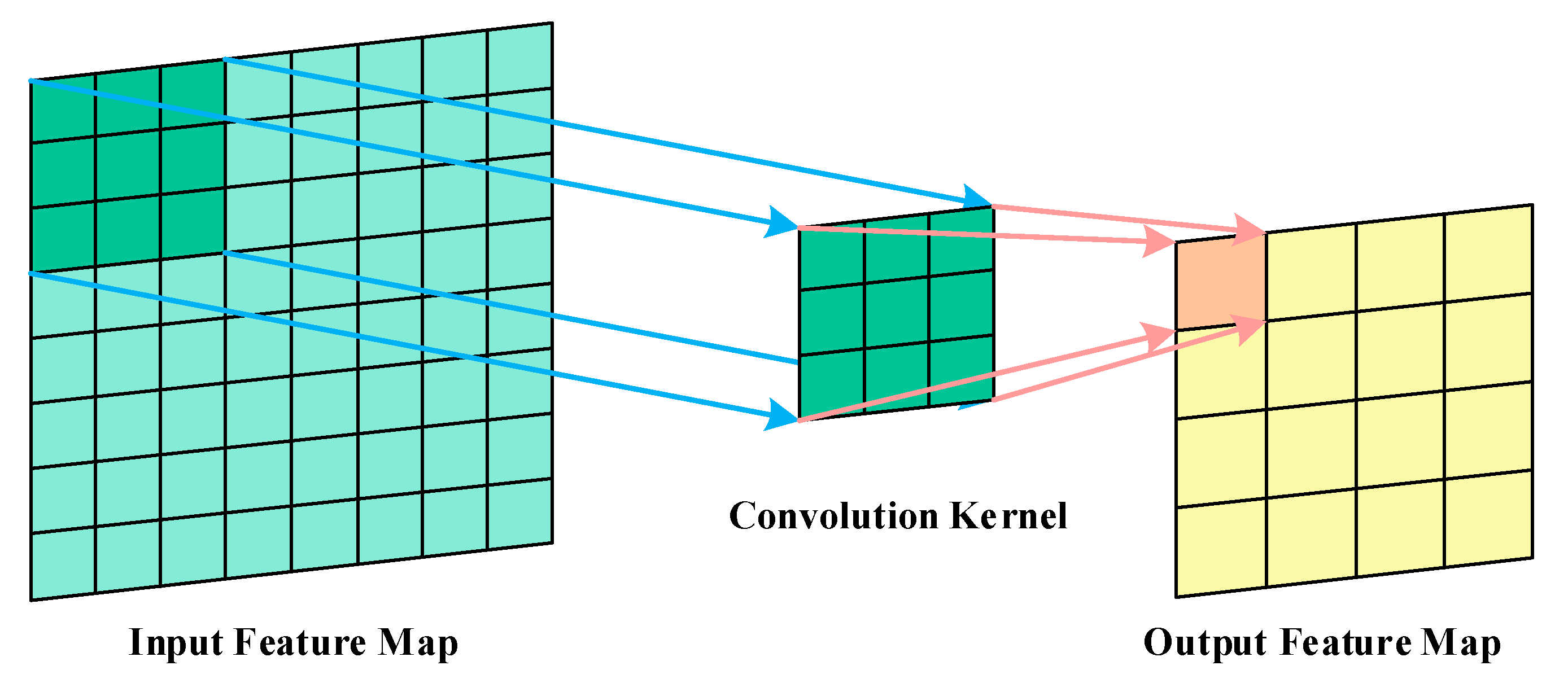
The 2DCNN can extract features from the previous layer, and its convolution kernel slides in the 2D direction, which is sensitive to spatial features such as edges and can be used to enhance the spatial feature information of the image. Figure 1 shows the feature extraction principle of 2D convolution. For the pixel corresponding to the position (p, q), the feature value of the point is equal to the cumulative sum of the products of the pixel value and the corresponding elements of the convolution kernel matrix. If the activation function is f, then the eigenvalue h_pq at (p, q) can be expressed as:

$$h_{pq}=f\left({\displaystyle \sum _{i,j}{\omega }_{ij}{x}_{\left(p+i\right)\left(q+j\right)}+b_1}\right)$$

(5)

The position (p + i, q + j) is in the area selected by the 2D convolution kernel (i, j), x refers to the input feature at different positions and is multiplied by ω_ij, which is the weight of the input in the position of the convolution kernel. $b_1$ is the bias term. The output feature map is smaller than the input feature map, and the side length Len is related to the input image side length W as well as the convolution kernel size F, which can be calculated as:

$$Len=W-F+1$$

(6)

2.3. Attention Mechanism

The proposal of an attention mechanism is to emphasize the interesting information among the numerous pieces of information, reducing the presence of useless information [35]. It has been widely used in image classification. Squeeze and excitation net (SENet) [13] and Efficient channel attention (ECA) [14] both were classic channel attention models with good classification performance, which learned the correlation between the channel features as the attention weights. There were also spatial attention mechanisms and spatial-spectral attention mechanisms [36,37,38,39,40]. The focus of spatial attention was the spatial position of the target in the image, and the spatial-spectral attention mechanism combined the advantages of spatial and spectral attention, which was more comprehensive and effective. Central vector-oriented self-similarity network (CVSSN) [41] calculated self-similarity for attention on deeper spatial features. Triple-attention residual networks (TARN) [42] paid more attention to associations between individual pixels during spatial feature extraction. Convolutional block attention module (CBAM) [15] is a representative spatial-spectral attention mechanism and has achieved remarkable classification results in the field of HSI, more attention mechanisms have been introduced into HSI classification. Meng et al. [43] proposed a novel dynamic spatial-spectral attention network (DSSAN) to adaptively adjust the spatial and spectral feature responses for more discriminative features. The coordinate attention module (CA) proposed by Hou et al. [44] creatively calculated the attention weight for horizontal and vertical input features and fused information among channels.

In recent years, Transformer [22] has become popular due to the proposal of a self-attention mechanism (SA). The self-attention in the Encoder module made full use of global information to train the model in parallel, and were combined in a multi-head self-attention module (MSA) to obtain the global correlation of input token sequences. Then, a Vision Transformer (ViT) [23] was proposed first to introduce Transformer to the vision domain, after which a series of studies were conducted to use Transformer in HSI classification tasks [45,46,47,48,49,50]. Huang et al. [51] utilized self-attention and cross-attention mechanisms to associate features of different samples with the same category. Tang et al. [52] recently proposed a double-attention transformer encoder (DATE) with two self-attention modules focusing on local spatial and global spectral features, respectively, and obtained great classification results. In general, the attention mechanisms mentioned above usually take image patches as the only input to calculate attention weights which will be put to input patches through global pooling and convolution processing. Only one form of input is considered, and information loss might arise during attention weights calculation, which can lead to a bias in the weights.

2.4. Methods

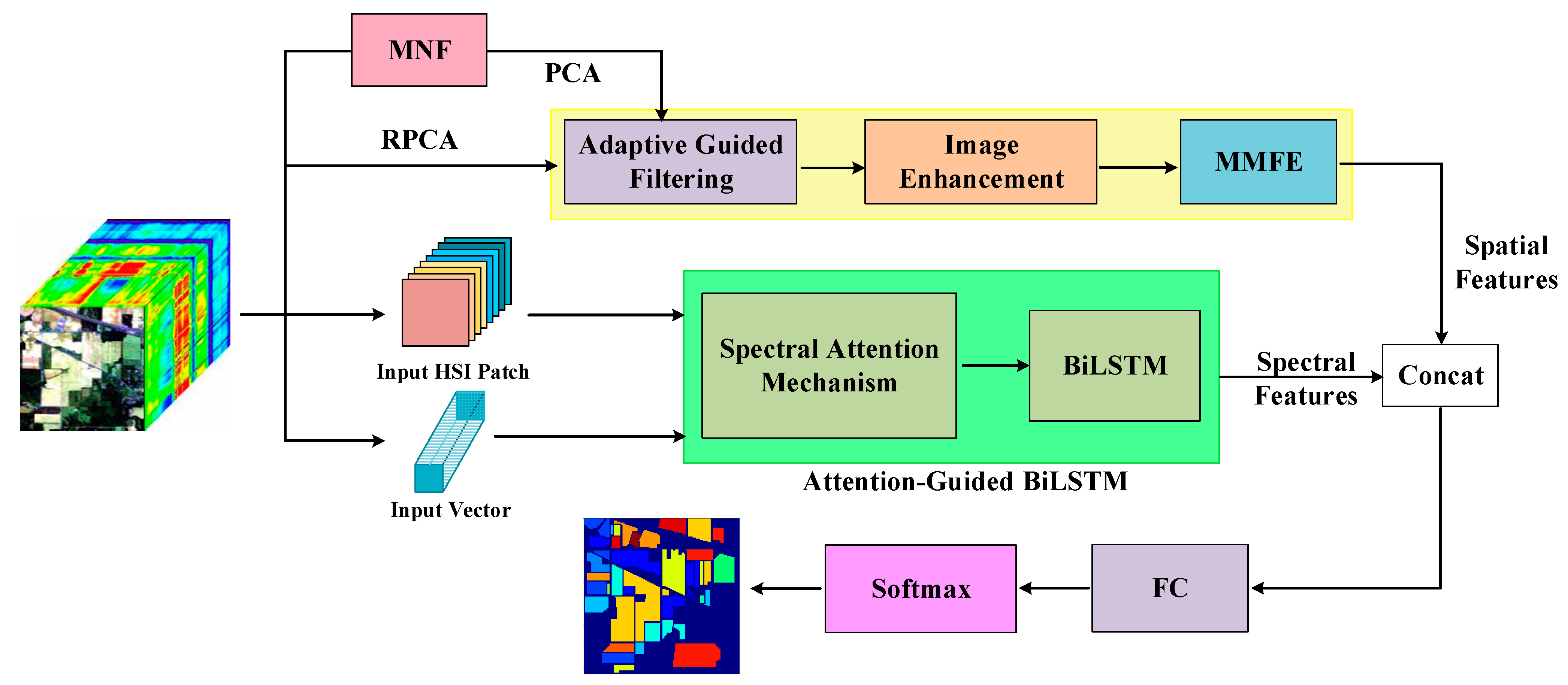
In this paper, we propose an improved feature enhancement and extraction model (IFEE) for hyperspectral image classification. The whole structure of IFEE is shown in Figure 2, the adaptive guided filtering module first helps to better retain the edge gradient information of input HSI and supplements some image information, after which spatial features are emphasized by the image enhancement module. To extract spatial features, we directly introduce the MMFE module proposed in SSDF [21] to obtain multiple features and spectral feature extraction is achieved through an attention-guided bidirectional sequential network. Extracted spatial and spectral features are concatenated and then classified.

2.4.1. Adaptive Guided Filtering Module

Traditional guided filtering [30] does well in retaining the edge gradient information of the input image by introducing the original image as the guiding image, which supplements the image information lost by filtering to a certain extent. Equations (1)–(4) explain the principle of traditional guided filtering, in which the coefficients a_k and b_k are obtained through Equations (3) and (4). However, traditional guided filtering can cause a halo during the smoothing operation on the boundary due to the fixed regularization coefficient λ in Equation (1). Specifically, the filtering operation on boundary region with high variance area can extract edge information very well with a_k closed to 1 and b_k closed to 0, while in smooth region with low variance, the values of a_k and b_k are expected to be 0 and the mean value within the guided filter window θ_k respectively. However, Equation (1) is unable to effectively adjust a_k and b_k across different regions. To avoid halos and retain clearer edge features, we introduce a guided filtering method called adaptive guided filtering that can adaptively adjust the regularization coefficients according to the guidance image through an edge ware weighting ${\phi }_k$ added to the same parameter λ in Equation (2) and the controlling parameter ${\gamma }_k$ to make a_k closer to 0 or 1. The definitions of the new energy function E′ and ${\phi }_k$, ${\gamma }_k$ are as follows:

$$E\left(a_k,d_k\right)={\displaystyle \sum _{i\in {\theta }_k}\left({\left(a_k{I}_i+d_k-s_i\right)}^2+\frac{\lambda }{{\phi }_k}{{\mathrm{a}}_k}^2\right)}$$

(7)

$${\phi }_k={\displaystyle \frac{1}{N}}{\displaystyle \sum _{i=1}^n\frac{{\chi }_k+\epsilon }{{\chi }_i+\epsilon }}, {\chi }_k={\sigma }_1\left(k\right){\sigma }_r\left(k\right)$$

(8)

$${\gamma }_k=1-{\displaystyle \frac{1}{1+e^{\eta \left({\chi }_k-{\mu }_i\right)}}}$$

(9)

where ε is set to (0.001 × L)² and $\eta$ in Equation (9) is a parameter calculated by ${\mu }_{\chi }$. ${\mu }_{\chi }$ is the mean of ${\chi }_k$ and ${\chi }_k$ is the combination of local variances of 3 × 3 window ${\sigma }_1\left(k\right)$ and (2r + 1) × (2r + 1) window ${\sigma }_r\left(k\right)$. N is the number of total pixels, and L means the gray value range of the input image.

Besides, we choose the image with robust PCA (RPCA) [53] processing as the guidance image while the image with minimum noise fraction rotation (MNF) [54] dimension reduction process is selected to be the input image. The addition of RPCA and MNF processing helps to denoise before filtering for better filtering results. As RPCA is not affected by the strength of noise on the assumption that the noise is sparse, while PCA is the opposite with its reliance on Gaussian noise assumptions, we choose RPCA with stronger anti-interference ability rather than PCA. Equation (10) summarizes the convex function optimization problem to be solved for RPCA processing.

$$\underset{A,R}{\min }{‖A‖}_{*}+\lambda {‖R‖}_1\hspace{1em}\hspace{1em}\hspace{1em}\mathrm{subject} A+R=D$$

(10)

where the low-rank matrix A with structural information and the sparse matrix R containing noise are decomposed from the image matrix D, and the sum of the nuclear norm of A and the 1-norm of R needs to be minimal. By removing R and keeping A as the guidance image of our adaptive guided filtering, the influence of noise can be greatly reduced.

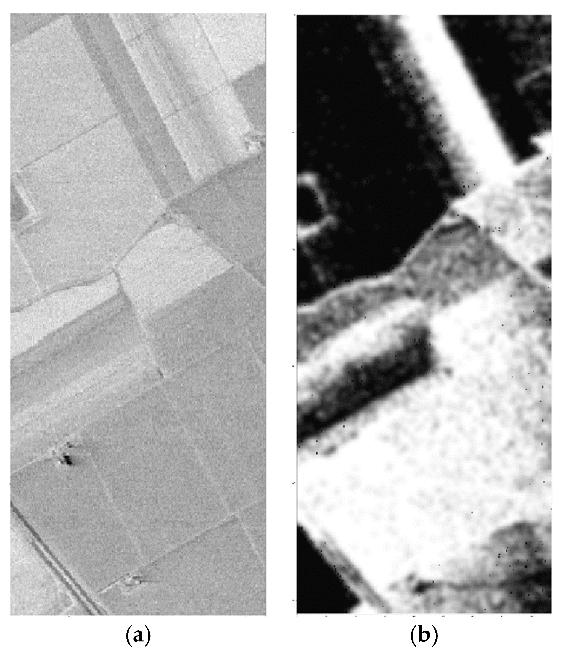
Specifically, we use PCA to reduce the dimensionality of the input HSI with MNF denoising before filtering for less computation. The adaptive guided filtering is conducted on each band of the images after dimensionality reduction by using the guidance image. Taking the Salinas Scene (SS) dataset as an example, Figure 3 shows the input and output image of the adaptive guided filtering module. By comparing the images before and after adaptive guided filtering processing, we can intuitively see that our adaptive guided filtering filters out certain noise which makes the image smoother, but the edges are clearer, indicating that the edge information is preserved.

2.4.2. Image Enhancement Module

The low spatial resolution of HSIs often makes it hard to obtain sufficient spatial features and details of ground objects, thus limiting the classification performance. For this problem, image enhancement methods can be used to improve the spatial resolution of HSI, which is convenient for subsequent feature extraction and fusion. We propose a lightweight image enhancement module composed of 2DCNNs in IFEE to improve the spatial resolution of the feature map after adaptive guided filtering processing, and the structure of the image enhancement module is shown in Figure 4.

In Figure 4, the whole image after adaptive guided filtering is regarded as the input cube P of the image enhancement module. P needs to go through a pre-processing stage first, where the image is shrunk by bicubic interpolation and then enlarged to obtain the feature map P+ with the same size but lower resolution compared with P. Compared to other interpolation methods, the bicubic interpolation image has more details and is smoother. The subsequent three-layer 2DCNN can successively extract the low-level spatial features from P+ and reconstruct them to obtain the feature map H with higher spatial resolution.

Table 1. Parameters in the image enhancement module.

Layer	Input	Convolution Kernel	Output
Conv1	$n_1\times n_2\times c\times 1$	$9\times 9\times c\times 64$	$n_1\times n_2\times 64\times 1$
ReLU1	$n_1\times n_2\times 64\times 1$	-	$n_1\times n_2\times 64\times 1$
Conv2	$n_1\times n_2\times 64\times 1$	$1\times 1\times 64\times 32$	$n_1\times n_2\times 32\times 1$
ReLU2	$n_1\times n_2\times 32\times 1$	-	$n_1\times n_2\times 32\times 1$
Conv3	$n_1\times n_2\times 32\times 1$	$5\times 5\times 32\times c$	$n_1\times n_2\times c\times 1$

lists the parameters of each 2D convolution layer and rectified linear unit (ReLU) layer in the proposed image enhancement module, all of which use 0-pixel edge padding operations to ensure that the input and output images have the same size. The second layer of 1 × 1 convolution is used to map the extracted low-resolution features to high-resolution image blocks through nonlinear mapping, and then these image blocks are aggregated through a 5 × 5 convolution layer to recover the high-frequency detail information lost before and reconstruct the output image H with higher spatial resolution than the input image P, so as to achieve image enhancement. It should be noted that using the low-dimensional image after adaptive guided filtering as the input of the image enhancement module can greatly reduce the computational complexity of the enhancement network and save time. Besides, we choose mean square error (MSE) between the output feature map H and the original guided filtered image P as the loss function to optimize the parameters of the network. The formula of the MSE loss function is as follows:

$$MSE={\displaystyle \frac{1}{M}}{\displaystyle \sum _{m=1}^M{\left({\mathrm{P}}_m-{\mathrm{H}}_m\right)}^2}$$

(11)

where m means the m-th pixel of the image, and M is the total number of pixels in the image.

2.4.3. Attention-Guided Bidirectional Sequential Spectral Feature Extraction Module

As for the extraction of spectral features, we use bi-directional long short-term memory (BiLSTM) [55], which is composed of forward and reverse LSTM. The image is input into two LSTM paths in the order of forward and reverse for feature extraction, and then the extracted spectral features from LSTM in different directions are concatenated correspondingly as the final output. Although LSTM makes up for the problem of gradient disappearance at farther positions in recurrent neural networks (RNN), there are still limitations in LSTM with one direction. Different from LSTM in one direction, BiLSTM considers all the information in the front and back directions and captures whether the position is near or far. Thus, the extracted spectral features are richer. Figure 5 shows the specific structure of BiLSTM, and the right side is the spectral feature extraction process of LSTM.

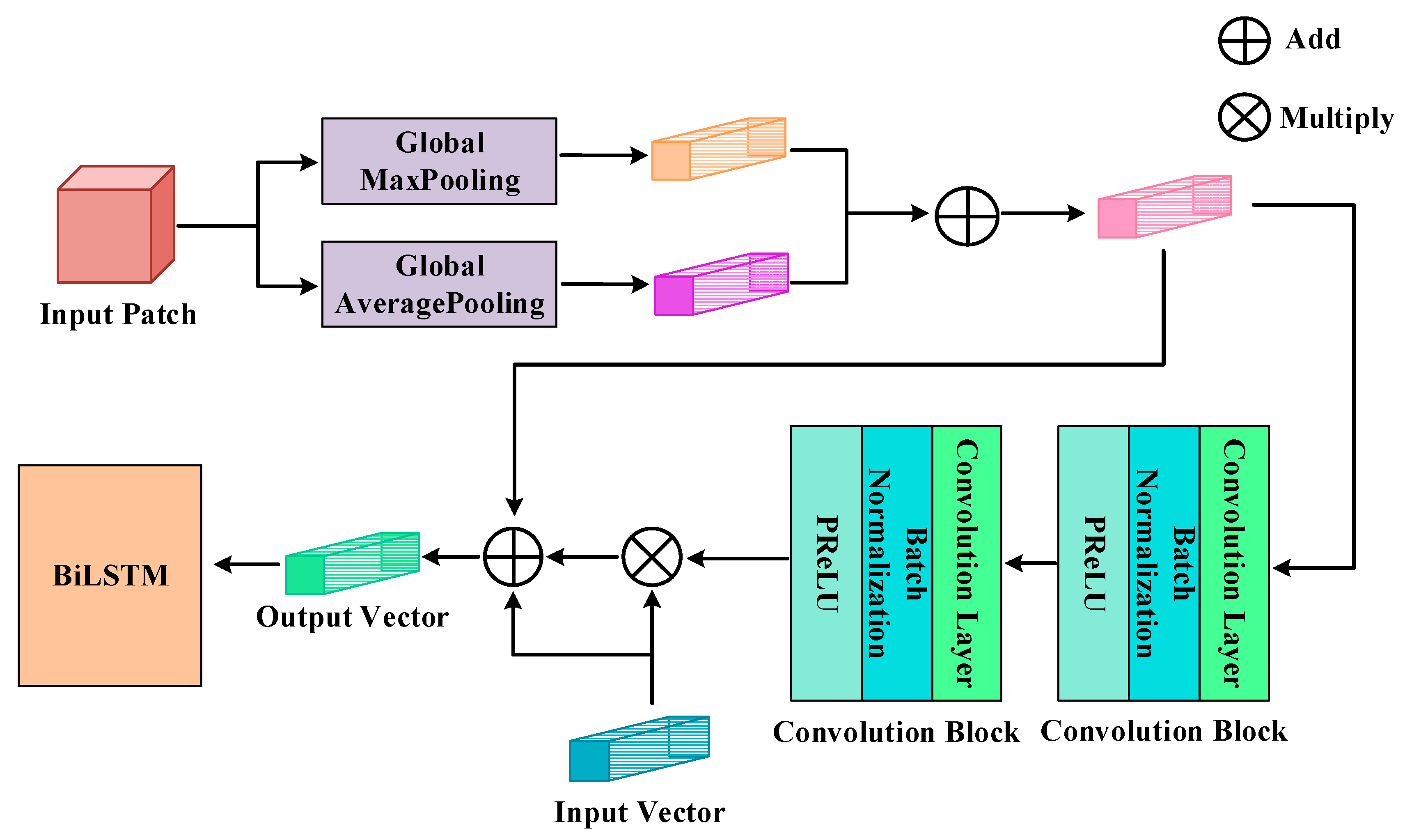
In order to further reduce the interference of noise as well as other factors and obtain important spectral information, we also design a spectral attention mechanism to emphasize the required spectral information and suppress irrelevant information before extracting features. Different from other attention mechanisms, there are two inputs in our spectral attention mechanism. One input is the patch taken from the original HSI dataset, and the other input is the vector sampled as sequences from the original HSI dataset. As shown in Figure 6, the principle of the attention mechanism can be expressed as

$$g=mp+ap$$

(12)

$$Z=Conv\left(Conv\left(g\right)\right)$$

(13)

$$Output=T\times Z+g+T$$

(14)

where mp and ap are the results of the input patch after global maximum pooling focusing on local features and global average pooling focusing on global features, respectively, and the addition of mp and ap can make features complementary. As Equation (12) shows, g is the combination of two kinds of pooling results mp and ap. Z means the channel attention weight obtained from g through two one-dimensional convolution processes, while T refers to the input vector, which is sampled from the original HSI and processed as a sequence.

The extraction of spatial features on spatial enhanced images is completed through the MMFE module proposed in [21]. There are four 3 × 3 2D convolutional layers in MMFE to obtain different hierarchical spatial features; a 2D convolution is added after each pooling layer to acquire more hierarchical features while changing the size of the feature map so that the feature maps of different levels have the same size after going through the convolutional layer. Let f be the activation function, p_i represents the output of each pooling layer, w_i and bi_i represent the corresponding weight matrix and bias item, respectively, the obtained i-th layer feature map Q_i can be calculated as Equation (15). The feature maps of each level are added in the added layer, after which they are stretched by the global average pooling (GAP) layer and output by the fully connected (FC) layer. MMFE performs deep feature extraction on the spatial features, and the obtained features are multi-level.

$$Q_i=f\left(w_i{p}_i+b{i}_i\right)$$

(15)

3. Results

3.1. Experimental Settings

Our experiments were conducted on a computer with a graphics card of NVIDIA GeForce GTX 1660 Super 6 GB, Intel Core i7-8700K CPU and memory of 16 GB. The software framework was Tensorflow 1.14.0 and the programming language was Python 3.6.13. Additionally, both RPCA and MNF were processed on MATLAB R2022a. The experiments select three widely used hyperspectral datasets to prove the effectiveness of our proposed method, including Indian Pines (IP), Pavia University (UP), Salinas Scene (SS). Each dataset is divided into training set, validation set and test set, the setting of validation set can prevent overfitting and improve the generalization ability of the model. We randomly select samples from each category of initial dataset in a certain proportion as the training set, then take samples in the same proportion with that of the training set from the remaining samples as the verification set, and the rest of samples are regarded as the test set. To discuss the performance of the proposed IFEE with fewer training samples, the proportion of training samples is set to 1% for larger datasets including UP and SS, while 3% for smaller IP dataset. We also discuss the classification performance under the condition of a small number of samples.

The epoch of experiment is set to 350, and the number of input images for adaptive guided filtering is selected from 25 and 20. We set the training times of the enhanced network as 10,000 and make the learning rate be 0.0001. All the patches used as the inputs of the proposed IFEE were in the size of 17. Batch size was set as 128. The patch size and batch size remained consistent across the three datasets. We also select some related classification methods with better effects as comparative methods, including SVM [3], LSTM [12], 3DCNN [11], MSCNN [9], SSFTT [20], HybridSN [19] and SSDF [21]. The main parameters of these comparative methods are consistent with those of the proposed IFEE, and the patch size in each comparative method is set to 17. SSDF introduces guided filtering and multi-scale spatial feature extraction for classification and achieves great results, but it takes quite a long time to process. In order to avoid random interference, we take the average of five experiments as the final results.

The evaluation indicators of experimental results include Overall Accuracy (OA), Average Accuracy (AA), and Kappa Coefficient (Kappa). OA measures the proportion of correctly classified samples out of the total number of test samples which provides an overall assessment of the classification performance across all classes. And AA refers to the mean accuracy rate of each category, evaluating the average classification performance across different classes. As a more robust indicator, Kappa has a better understanding of how well the model’s predictions align with the actual class labels.

3.2. Datasets

The IP dataset was captured at the Indian Pine test site in northwest Indian, including 224 spectral reflection bands with the size of 145 × 145, and the wavelength range was 0.4~2.5 μm. The existing ground-truth are divided into 16 classes, and are not entirely mutually exclusive. UP dataset was obtained during an air race over Pavia in northern Italy, including 115 spectral reflection bands with the size of 610 × 340. The existing ground-truth are divided into 9 classes, including trees, bricks, meadows, and so on. As for SS dataset, the scene was captured by a 224-band sensor over the Salinas Valley in California, featuring a high spatial resolution. As in the Indian Pines scene, 20 water absorption bands were discarded. The existing ground-truth are divided into 16 classes, with 54,129 samples in total. More detailed information about these datasets is described in [56].

From

Table 2. The details of IP dataset with 3% training samples.

Class	Category	Training	Validation	Test
1	Alfalfa	2	2	42
2	Corn	43	43	1342
3	Corn-mintill	25	25	780
4	Corn	8	8	221
5	Grass-pasture	15	15	453
6	Grass-tree	22	22	686
7	Grass-pasture-moved	1	1	26
8	Hay-windrowed	15	15	448
9	Oats	1	1	18
10	Soybean-notill	30	30	912
11	Soybean-mintill	74	74	2307
12	Soybean-clean	18	18	557
13	Wheat	7	7	191
14	Woods	38	38	1189
15	Buildings-Grass-Trees-Drives	12	12	362
16	Stone-Steel-Towers	3	3	87
Total		314	314	9621

,

Table 3. The details of UP dataset with 1% training samples.

Class	Category	Training	Validation	Test
1	ASphalt	67	67	6497
2	Meandows	187	187	18,275
3	Gravel	21	21	2057
4	Trees	31	31	3002
5	Painted metal sheet	14	14	1317
6	Bare Soil	51	51	4927
7	Bitumen	14	14	1302
8	Self-Blocking Bricks	37	37	3608
9	Shadows	10	10	927
Total		432	432	41,912

and

Table 4. The details of SS dataset with 1% training samples.

Class	Category	Training	Validation	Test
1	Brocoli_green_weeds_1	21	21	1967
2	Brocoli_green_weeds_2	38	38	3650
3	Fallow	20	20	1936
4	Fallow_rough_plow	14	14	1366
5	Fallow_smooth	27	27	2624
6	Stubble	40	40	3879
7	Celery	36	36	3507
8	Grapes_untrained	113	113	11,045
9	Soil_vinyard_develop	63	63	6077
10	Corn_senesced_green_weeds	33	33	3212
11	Lettuce_romaine_4wk	11	11	1046
12	Lettuce_romaine_5wk	20	20	1887
13	Lettuce_romaine_6wk	10	10	896
14	Lettuce_romaine_7wk	11	11	1048
15	Vinyard_untrained	73	73	7122
16	Vinyard_vertical_trellis	19	19	1769
Total		549	549	53,031

, we can see the details of each dataset used in our experiments.

3.3. Experimental Results

Table 5. Classification results on the IP dataset.

Class	SVM	3DCNN	LSTM	MSCNN	HybridSN	SSDF	SSFTT	IFEE
1	8.61	42.22	23.53	70.22	16.89	95.67	36.44	97.66
2	63.84	67.79	64.84	94.65	80.71	90.76	86.99	91.75
3	51.89	56.23	61.06	91.02	84.57	91.58	89.42	93.46
4	25.04	47.39	42.17	84.61	70.96	92.77	92.52	93.57
5	69.85	78.42	91.77	82.09	94.88	90.27	97.23	95.37
6	86.83	94.19	79.66	98.39	97.85	97.31	97.20	95.34
7	0.00	0.00	25.00	0.00	55.56	57.59	100.00	47.87
8	98.41	97.28	82.24	98.06	99.96	98.98	98.66	99.78
9	0.00	0.00	0.00	0.00	91.58	78.53	93.68	96.98
10	65.56	67.34	73.38	87.85	89.65	94.62	93.04	95.63
11	74.37	75.35	65.86	96.59	95.22	97.78	98.16	98.26
12	42.57	43.23	56.11	87.99	64.90	82.85	82.61	87.88
13	90.45	87.64	80.25	98.39	81.71	97.53	94.27	97.43
14	92.39	93.52	88.71	99.85	98.53	99.27	98.94	98.34
15	33.28	51.84	50.25	85.23	85.83	94.71	92.73	93.65
16	45.05	76.04	86.56	99.34	72.22	88.04	77.78	92.85
OA (%)	69.13	73.09	71.24	93.22	88.99	94.30	93.64	95.42
	1.02	1.68	0.01	0.91	1.11	1.83	0.68	0.16
AA (%)	52.97	61.16	60.71	79.43	80.06	90.52	89.36	92.03
	0.93	3.35	0.04	0.84	1.47	1.49	1.88	0.65
Kappa (×100)	64.58	69.25	66.90	92.24	87.40	93.51	92.73	94.78
	1.10	2.00	0.01	1.04	1.23	2.08	0.78	0.19

,

Table 6. Classification results on UP dataset.

Class	SVM	3DCNN	LSTM	MSCNN	HybridSN	SSDF	SSFTT	IFEE
1	86.98	86.18	80.84	97.22	93.43	97.10	90.50	97.54
2	97.57	96.91	85.43	99.17	99.53	98.86	99.57	99.68
3	50.95	55.48	53.80	86.53	83.88	93.39	92.94	94.47
4	86.57	91.40	91.02	93.44	80.38	97.86	73.53	97.63
5	98.77	98.32	97.18	99.86	99.85	99.00	96.88	95.41
6	71.62	64.52	63.92	98.96	99.14	97.24	100.00	99.42
7	77.89	66.58	49.61	95.52	97.51	80.97	96.70	99.62
8	85.61	88.48	73.75	91.56	82.02	86.41	96.55	94.80
9	99.83	91.88	99.13	91.43	68.71	97.64	61.13	92.38
OA (%)	88.25	87.27	80.51	96.89	94.16	96.20	94.74	98.19
	0.66	0.98	0.01	0.69	0.90	0.19	1.58	0.22
AA (%)	83.98	82.19	77.19	94.86	89.38	94.27	89.76	96.77
	1.80	1.53	0.01	0.85	1.57	0.77	1.59	0.67
Kappa (×100)	84.21	82.88	73.78	95.88	92.22	94.96	93.02	97.59
	0.92	1.36	0.01	0.92	1.20	0.26	2.06	0.29

and

Table 7. Classification results on SS dataset.

Class	SVM	3DCNN	LSTM	MSCNN	HybridSN	SSDF	SSFTT	IFEE
1	98.58	85.54	98.68	99.98	99.76	99.47	99.95	100.00
2	98.19	99.49	98.96	100.00	99.99	99.90	100.00	99.50
3	94.05	94.50	85.03	95.91	99.60	97.59	99.78	99.18
4	96.54	96.29	97.61	97.45	99.42	99.31	99.36	98.81
5	96.55	97.20	95.93	97.63	98.94	99.05	98.36	97.68
6	99.23	98.35	99.85	99.66	99.54	99.66	99.99	99.98
7	99.51	97.05	93.57	99.60	99.93	98.33	99.93	100.00
8	86.30	83.41	75.72	94.32	95.54	95.97	98.71	99.12
9	99.39	98.10	97.93	99.77	99.99	99.48	99.99	99.69
10	87.58	87.22	83.72	95.22	98.76	98.89	98.88	99.63
11	89.81	90.55	77.57	94.67	98.22	86.76	98.75	97.52
12	98.31	96.68	95.99	98.78	99.79	99.65	99.95	96.75
13	97.95	95.46	90.24	93.30	90.80	96.51	96.87	99.19
14	90.57	93.68	97.63	87.22	97.26	94.83	98.47	99.62
15	62.23	74.29	71.26	88.91	90.70	94.22	95.24	97.39
16	91.67	83.81	94.09	98.96	99.32	98.79	99.34	99.99
OA (%)	89.75	89.73	87.58	96.05	97.34	97.47	98.78	99.08
	0.53	1.02	0.01	0.25	0.17	0.72	0.36	0.04
AA (%)	92.90	91.98	90.86	96.25	97.97	97.40	98.97	99.11
	0.75	1.09	0.01	0.63	0.67	0.68	0.39	0.20
Kappa (×100)	88.56	88.58	86.16	95.60	97.04	97.18	98.64	98.98
	0.60	1.13	0.01	0.28	0.18	0.81	0.40	0.05

show the classification results of the proposed method on the three datasets, as well as the experimental results of the corresponding comparative methods. We can see that the proposed method has the highest OA, AA, and Kappa among all the comparison methods for each dataset. Figure 7, Figure 8 and Figure 9 list the classification results of IFEE and various comparison methods on the IP, UP, and SS datasets, making it more intuitive to see the stand and fall of classification results. As an effective method for HSI classification, SSDF outperforms other comparison methods on the IP and UP datasets, which makes it a competitive method for the proposed IFEE. Therefore, we will pay more attention to SSDF during the analysis of experimental results.

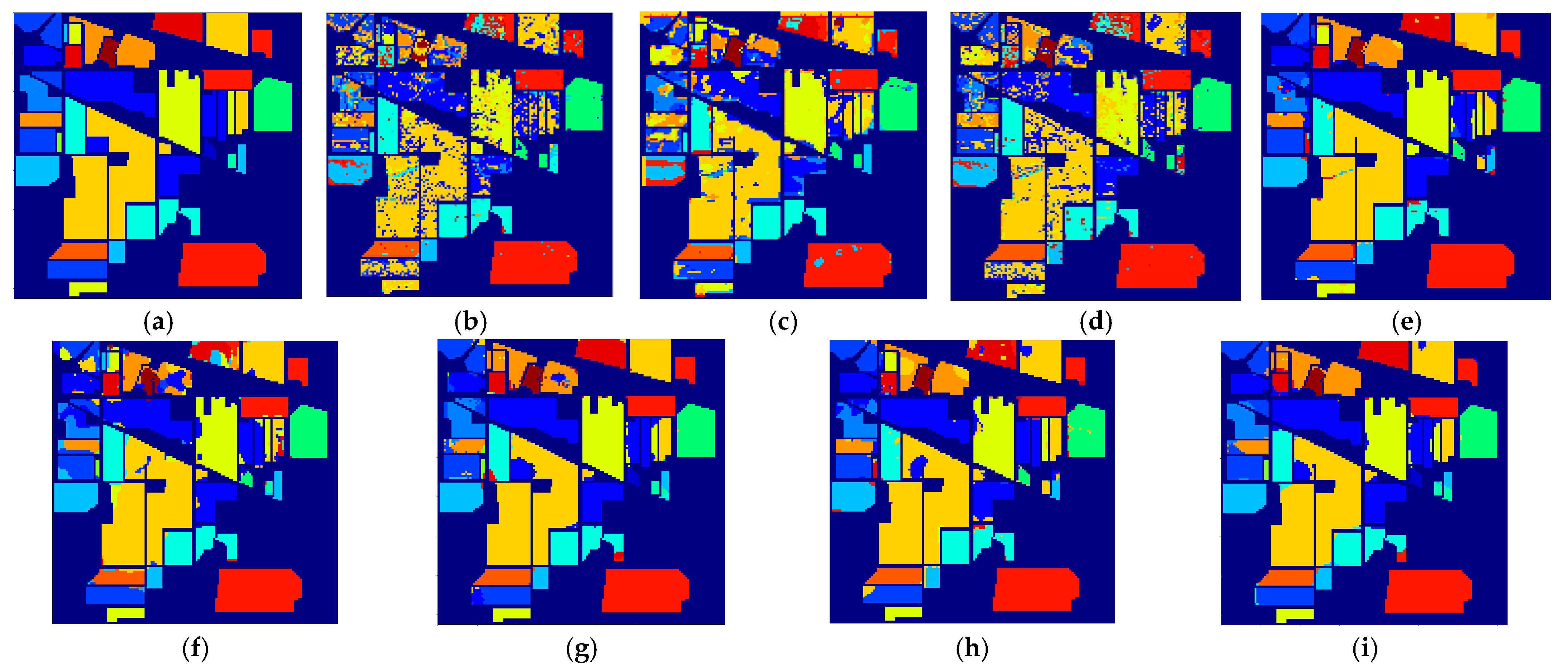
It can be seen from the experimental results on IP in Table 5 that IFEE performs the best in three evaluation indicators with the value of 95.42%, 92.03% and 94.78% compared with other methods. Although IFEE does not achieve the highest classification accuracy on some categories, it shows a better classification effect on categories 1, 3, 4, and 10, where other methods generally don’t perform very well, and the classification accuracy is greatly improved as the highest. Compared with SSDF, the classification results of IFEE in most categories have certain improvements, and the OA, AA, and Kappa of IFEE have a significant improvement of 1.12%, 1.51%, and 1.27%, respectively. It’s probably because the spectral attention mechanism in IFEE helps extract more beneficial spectral features for classification, thus providing more abundant features for network training than SSDF. And the image enhancement module also plays a significant role in better spatial feature extraction. Figure 7 lists the classification maps of all methods on IP dataset. As the number of samples in the IP dataset is quite small and 3DCNN does not make full use of the spectral information, it is easy to explain the large misclassification areas in the classification map of 3DCNN. There are also obvious misclassified pixels in the maps of LSTM, MSCNN and HybridSN, while SSDF, SSFTT, and IFEE having clearer areas classification. However, IFEE has the least misclassification at the bottom boundary and gets the best classification results. The reason could be the adaptive guided filtering of IFEE helps to preserve more edge information for classification.

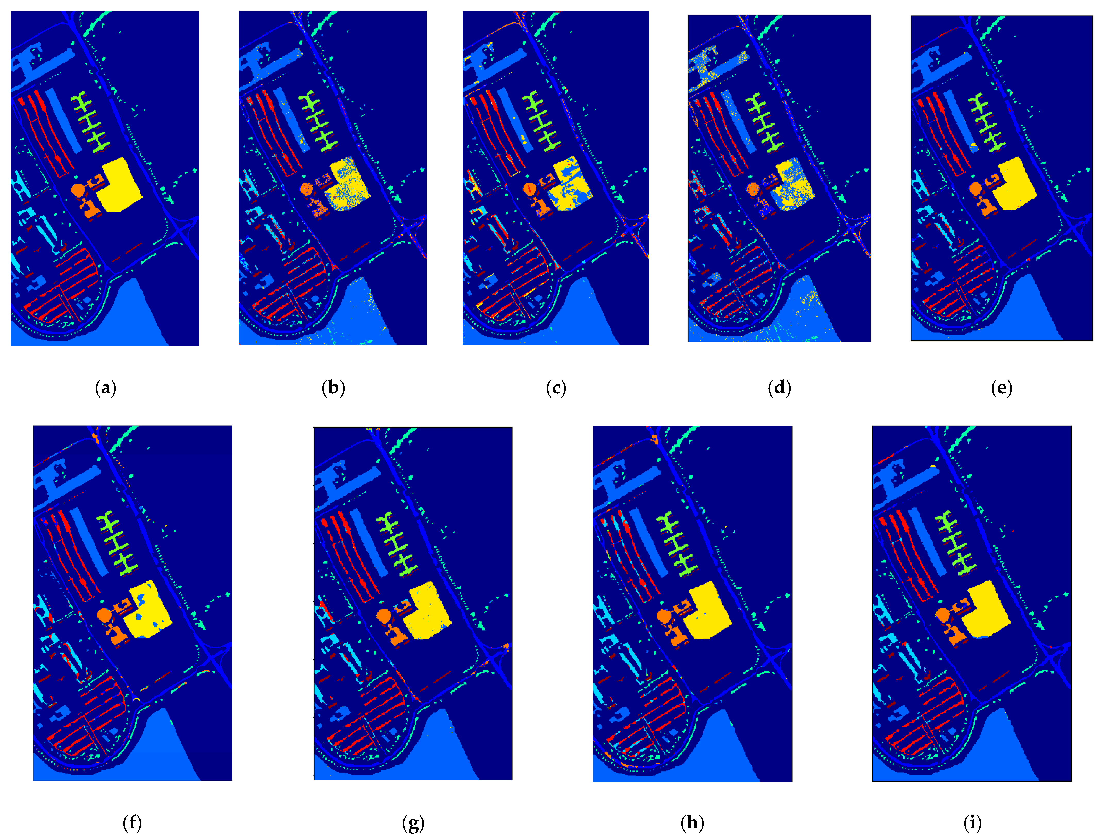
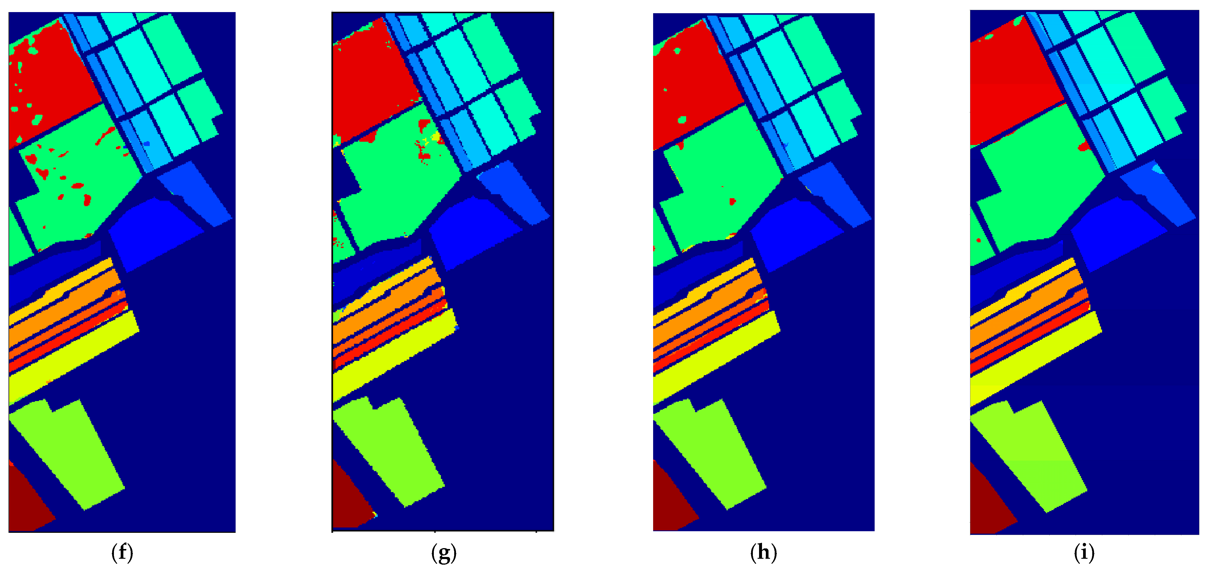
Figure 8 lists the classification maps of all methods on the UP dataset. There are many misclassifications around green and yellow areas in most comparison methods, which is difficult to classify with a small training set. However, MSCNN, SSFTT, and IFEE do well in these areas with a clear yellow area and edge, among which IFEE acquires the best classification map considering the classification color blocks of other detailed and small areas. From Table 6, we can see that the proposed IFEE achieves the highest OA, AA, and Kappa on the UP dataset with 98.19%, 96.77%, and 97.59%, revealing that the overall classification performance of IFEE is excellent compared with other classic methods. It is worth mentioning that the values of evaluation indicators obtained by IFEE and MSCNN are close, mainly because MSCNN uses multi-scale convolution kernels to capture feature information of different scales simultaneously; the multi-scale features enable the network to extract and utilize the key features effectively even when the number of labeled samples is limited. However, IFEE specifically considers the introduction of spectral features during classification, which is lacking in MSCNN, and the variances of the proposed IFEE in the three indicators are much smaller than that of MSCNN, indicating that IFEE has more advantages in stability. In addition, IFEE can maintain relatively good classification results for each category, which is very balanced, even though the classification accuracy for very few categories is slightly lower than the best. Based on the above analysis, IFEE still has significant advantages over other methods.

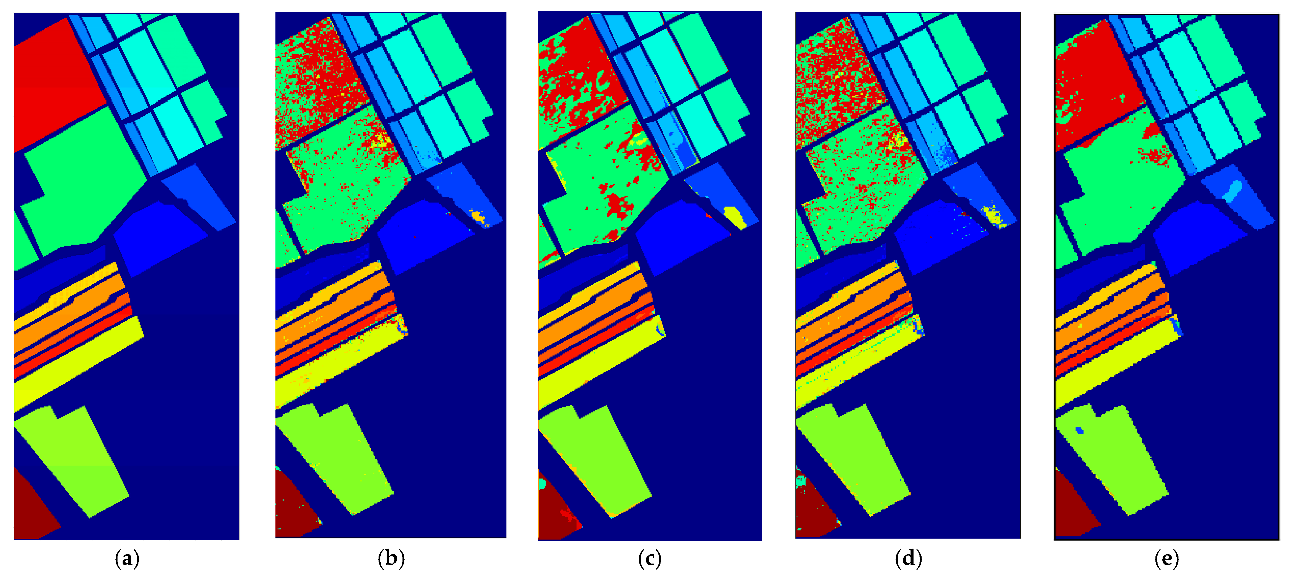
Table 7 shows all classification results of comparison methods on the Salinas dataset. We can see that the IFEE model achieves an average OA, AA, and Kappa of 99.08%, 99.11%, and 98.98%, outperforming the SSDF and SSFTT models, which perform the best among comparison methods by 1.61% and 0.30%, respectively. Specifically, it can be seen that IFEE achieves the highest classification accuracy in most categories, especially in class 8 and class 14, which were difficult to classify. The variance values of the evaluation indicators shown in Table 7 are the smallest, proving the stability of the proposed IFEE. Such classification effect can be seen more intuitively from the classification result maps listed in Figure 9. It can be found that the adjacent red and green areas in classification maps are very prone to misclassification, and a large area of pixels with incorrect classification still obviously appears in the classification maps of most comparison methods. However, we can only see several small patches with wrong classification pixels in the classification map of IFEE on the SS dataset, which has great accuracy and visual effect overall. Although SSDF also introduces guided filtering and has quite good classification effects on the SS dataset, the adaptive guided filtering in IFEE can adjust the regularization parameter of guided filtering according to the changes of pixel values in the image and the boundary information of both local and global ranges can be well preserved. The image enhancement module in IFEE helps to supplement the detailed information, contributing to the good performance of IFEE as well.

In general, the classification performance of IFEE on the three datasets is significantly better than traditional machine learning methods, and it is also highly competitive compared with the current excellent hyperspectral image classification methods based on deep learning. The introduced guided filtering and image enhancement operations optimize spatial features before they are input to the classification network, while the attention-guided BiLSTM module also enhances the extraction of spectral information. These processes help ease the learning of features by the classification network burden while also improving learning efficiency and classification accuracy.

4. Discussion

4.1. Effectiveness of Dual-Branch Structure

Our proposed IFEE is a dual-branch structure model, which combines the spatial information and spectral information extracted from two separate branches respectively. Theoretically speaking, the information that can be obtained by a single-branch structure is very limited. A dual-branch structure that combines different types of features often extracts richer and more comprehensive information than a single-branch structure. Therefore, it should be easier for the dual-branch structure to get better performance in classification tasks. So, we split the spatial branch and spectral branch of IFEE into two single-branch models and conducted experiments on the IP, UP and SS datasets respectively. By comparing the experimental results with the original IFEE method, it can be found that the experimental results on both the spatial single branch and spectral single branch have a large gap with that of the dual branch, confirming the dual branch structure adopted by IFEE has higher classification accuracy. The results are listed in

Table 8. The OA (%) results of experiments on the dual-branch structure of IFEE.

Methods	IP	UP	SS
Spatial Branch	94.65	97.51	98.77
Spectral Branch	75.63	83.63	92.23
IFEE	95.42	98.19	99.08

.

The results in Table 8 reveal that our proposed IFEE with dual-branch structure has a better performance than each single branch of IFEE on all three datasets, with the OA of 95.42%, 98.19% and 99.08%, respectively. The spectral branch concentrates on spectral feature extraction and does not fully utilize the spatial features, thus obtaining quite low classification accuracy. Meanwhile, the spatial branch already has great classification results with the combination of guided filtering and enhancement modules. It achieves an improvement of 19.02%, 13.88%, and 6.54%, respectively, on OA compared with the spectral branch. Still, the spectral information supplemented by the dual-branch structure can further improve the classification accuracy on the basis of the spatial branch. Therefore, it is effective and necessary to choose the dual-branch structure rather than a single branch for better classification results.

4.2. Effectiveness of Different Modules

To verify the effectiveness of different modules in our proposed structure, we perform various combinations of main modules including adaptive guided filtering (AGF) module, spatial image enhancement (SIE) module, BiLSTM with spectral attention mechanism (Bi + SAM) module, and compare the experimental results of combined structures on three datasets. As MMFE [21] is an existing module used as the basic feature extraction module in the proposed IFEE, we do not discuss about its effectiveness. The OA results can be shown in

Table 9. The OA (%) results of experiments on the module construction of IFEE.

AGF	SIE	Bi + SAM	IP	UP	SS
×	√	√	93.86	93.40	94.89
√	×	√	95.05	97.77	98.96
√	√	×	94.65	97.51	98.77
√	√	√	95.42	98.19	99.08

, where × indicates the corresponding module is not included, and √ means this module is included. The abbreviations of each module are used in the Table 9.

As we can see from Table 9, removing any module can result in a decrease in OA on all datasets, which proves that all the three modules are beneficial for classification results. By comparing the differences in classification results among different rows in Table 9, we can demonstrate the effectiveness of each module in the classification network structure. Since the BiLSTM with spectral attention mechanism module forms the spectral branch of IFEE, the structure removing Bi + SAM module from the IFEE network is equivalent to the spatial branch of IFEE which is mentioned earlier in Table 8. The introduction of Bi + SAM module implies the extraction of spectral features leading to a significant improvement in classification results. The comparison results of OA in Table 9 confirm this trend, showing that independently adding this module can improve the OA on the three datasets by 0.77%, 0.68% and 0.31%, respectively. Next, we will analyze the effectiveness of the guided filtering and spatial image enhancement modules.

Effectiveness of Guided Filtering. The guided filtering module is designed for denoising and smoothing on the input HSI while preserving certain edge information. The process of this module prepares for subsequent enhancement and extraction of spatial features with greater specificity for classification. The first and fourth rows of Table 9 precisely constitute a set of comparative experiments regarding to the effectiveness of the guided filtering module. When the guided filtering process is removed, the spatial image enhancement is directly applied to the original HSI input without altering other parts of the network. The changes in OA on the three datasets before and after removing the guided filtering module indicate that enhancing and classifying the guided filtered image is more effective than performing post-processing on the input HSIs directly. The improvement of OA can achieve up to 4.97%, suggesting that the introduction of the guided filtering module can significantly improve the classification accuracy.

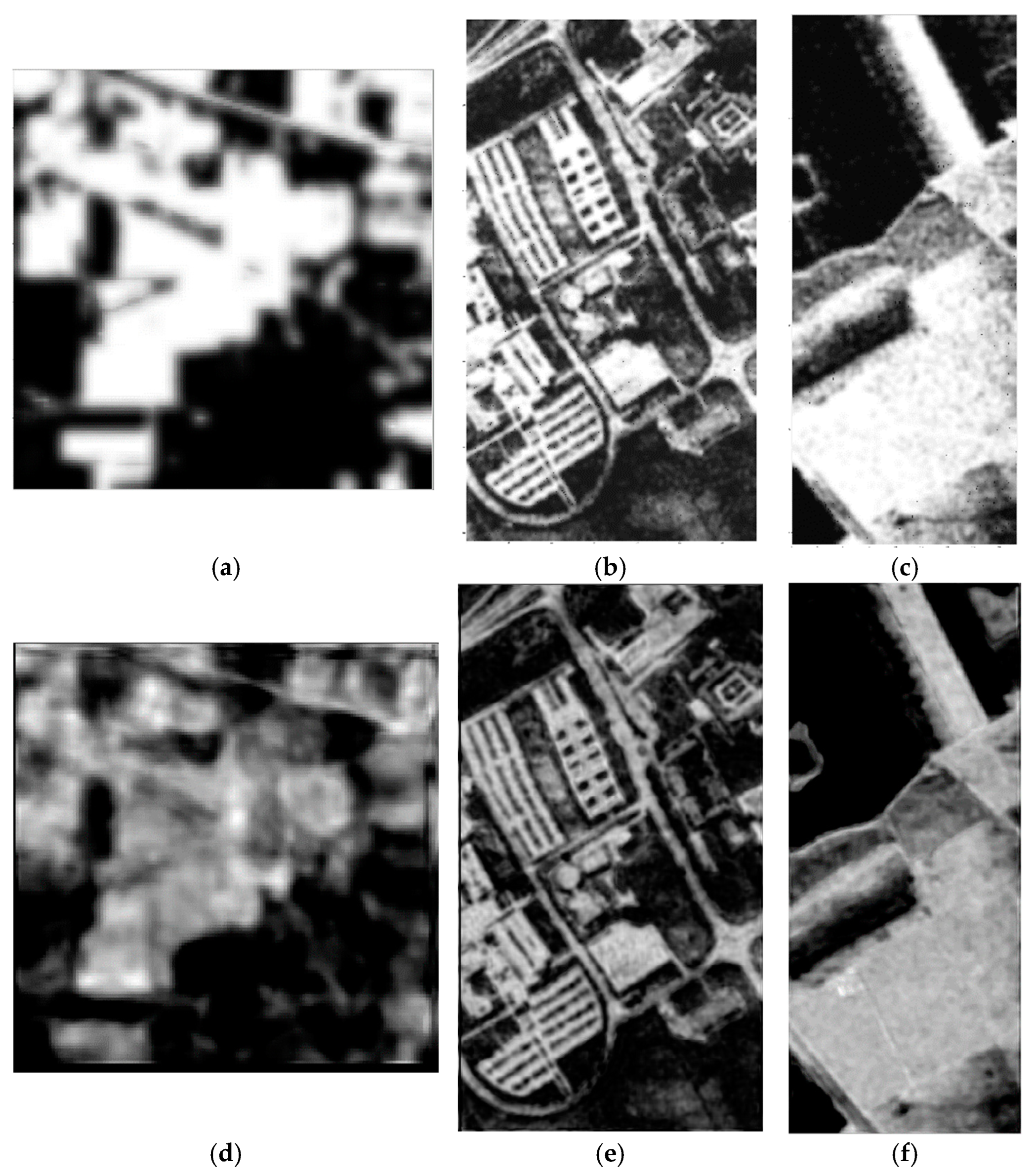
Effectiveness of Spatial Image Enhancement. In our proposed method, the introduction of spatial image enhancement also plays an important role in improving the HSI classification results. By comparing the classification results in the second and fourth rows of Table 9, which correspond to the IFEE method without the spatial image enhancement module and complete IFEE method respectively, the effectiveness of spatial image enhancement module can be proved on IP, UP and SS datasets. In the absence of the image enhancement module, there is a decrease of 0.12–0.42% in OA on IP, UP and SS datasets. Although the magnitude is not significant, this trend indicates that SIE module is beneficial for achieving better classification results with spatial features enhanced. To more intuitively demonstrate the effect of the image enhancement module, we choose the first channel of feature matrix to draw a 2D gray image as the visualization of feature processing effects. Figure 10 compares the 2D gray images before and after enhancement processing on all three datasets. Each image after enhancement is clearer and more colorful than before, with more obvious partitions of different colors. It can be concluded that the joining of spatial image enhancement is necessary and beneficial for classification.

In the collocation of modules, the best OA can be obtained on all datasets only if all modules are present, which indicates that the network construction of IFEE is reasonable and efficient.

4.3. Analysis of BiLSTM with Spectral Attention Mechanism Module

Next is the further analysis of the spectral branch part composed of the BiLSTM with spectral attention mechanism module. We first verify the effectiveness of the spectral attention mechanism and BiLSTM through two sets of experiments: one is to compare IFEE before and after removing the spectral attention mechanism, and the other is to compare IFEE and IFEE without BiLSTM which only has the spectral attention mechanism part for spectral information processing. By comprehensively comparing the classification results of these two sets of experiments, it can be determined whether the spectral attention mechanism and BiLSTM are helpful in improving the classification accuracy at the same time.

Table 10. The OA (%) results of experiments on IFEE without SAM or BiLSTM, IFEE with LSTM instead of BiLSTM, and IFEE.

Methods	IP	UP	SS
IFEE × SAM	95.35	98.14	98.82
IFEE × Bi	95.21	97.97	98.68
IFEE × Bi + LSTM	94.78	97.27	98.79
IFEE	95.42	98.19	99.08

lists the OA results of IFEE without the spectral attention mechanism or BiLSTM on IP, UP, and SS datasets; the experimental models are named by abbreviation, where IFEE × SAM stands for IFEE without the spectral attention mechanism (SAM), IFEE × Bi stands for IFEE without BiLSTM (Bi), IFEE × Bi + LSTM means replacing the BiLSTM part of IFEE with LSTM.

As for the first set of comparison experiments, we can compare the OA results of IFEE without spectral attention mechanism and IFEE in Table 10. From Table 10, it can be seen that without the spectral attention mechanism, the accuracy of classification drops about 0.05% to 0.26%, revealing that the attention mechanism contributes to better classification results. Though there is rich spectral information in HSIs, noises, and interferences still exist. The spectral attention mechanism helps to pick the spectral bands with more feature information from multiple bands, which suppresses irrelevant channels and avoids noise interference, thus making BiLSTM extract more needed spectral information. Therefore, the proposed IFEE with the spectral attention module can achieve better classification performances as richer spectral features being extracted. The experimental results show that it is necessary and effective to introduce the attention mechanism to assign weights to different spectral channels, which can help improve the performance of classification.

The results of the second set of comparison experiments are the OA results of IFEE without BiLSTM and IFEE in Table 10, which can validate the effectiveness of BiLSTM. When BiLSTM is removed from the original IFEE structure, the classification results on the IP, UP, and SS datasets decrease by 0.21%, 0.22%, and 0.40%, respectively. Besides, removing BiLSTM module from IFEE causes a greater decline in OA values than removing the SAM module. The reduction of OA provides intuitive evidence that the addition of BiLSTM to the overall network can enhance the accuracy of classification results. Since BiLSTM plays a significant role in the long-term tracking of effective spectral information in the spectral branch, more distinguishable spectral features can be extracted for classification.

BiLSTM is composed of forward and reverse LSTM and considers the information in two directions captures whether the position is near or far, while LSTM only contains information in a single direction. Therefore, the use of BiLSTM in the network should be more effective than using LSTM. To support this conclusion, we cautiously conduct an additional experiment by replacing the BiLSTM component in IFEE with LSTM and reported the classification results in Table 10. It can be observed that after replacing BiLSTM with LSTM in IFEE, the OA declines and is worse than the OA of IFEE with only BiLSTM in spectral branch, further confirming the effectiveness of BiLSTM.

We know that the inputs of BiLSTM are usually sequences. But the inputs of BiLSTM with spectral attention mechanism module in our proposed method are segmented patch blocks, which are processed by the attention mechanism part and converted into a sequence format to feed into BiLSTM. So, what would the experimental results be under the same structure if we serialize the HSI and input sequences into this module?

To explain the problem, we first carried out the experiments on the spectral branch of IFEE with a single-branch structure, using sequences and patch blocks as the inputs, respectively. In

Table 11. The OA (%) results of experiments on the input types of BiLSTM with spectral attention mechanism module.

Methods	IP	UP	SS
SB-P	75.63	83.63	92.23
SB-S	56.35	73.76	65.10
IFEE-P	95.42	98.19	99.08
IFEE-S	94.94	97.82	98.83

, methods SB-P and SB-S refer to the spectral branch of IFEE with patch block input and sequence input, respectively. As shown in Table 11, when patch blocks are used as inputs on the spectral branch, the OA values on all three datasets are higher than those of the sequence inputs. Such gap in classification results is more evident on the SS dataset, where there is an 27.13% improvement in OA when using patch blocks as inputs. Subsequently, we conducted experiments in our proposed dual-branch IFEE network structure, using patch blocks and sequences as the inputs to the spectral branch respectively while combining them with the spatial branch. The experimental results under the dual-branch structure are also listed in Table 11, where methods IFEE-P and IFEE-S stand for IFEE with patch block input and with sequence input, respectively. Similarly, it can be seen from Table 11 that although the differences in classification results of IFEE with dual-branch structure with the two types of inputs is not so notable on three datasets, the classification performance is generally better when patch blocks are used as the inputs of the spectral branch, which is consistent with the experimental results of spectral branch of IFEE with single-branch structure. This may be because converting HSI into a sequence format can disrupt the spatial relationship between neighboring pixels, thus resulting in the inability to fully utilize the spatial structural relationship between pixels. However, the patch blocks obtained by dividing the HSI retain certain spatial structural information and complement local features for classification. Therefore, using patch blocks as the inputs of the BiLSTM with spectral attention mechanism module achieves better classification results and is a superior choice.

4.4. Performance under Limited Labeled Samples

To discuss the performance of the proposed IFEE with fewer training samples, we designed a group of experiments that only selected a small number of labeled samples as the training set. 3%, 5%, 8%, and 10% of labeled samples were extracted as the training set on the IP dataset, and the training set division ratios on UP and SS datasets are 1%, 3%, 4%, and 5%, respectively. We also conducted another set of experiments, considering situations closer to the problem of insufficiently labeled samples. The training set is obtained by selecting 5, 10, 15, and 20 labeled samples from each class. There are discussions about the classification performance of the proposed IFEE and various comparison methods under different training set division ratios as well as with different numbers of training samples in each class. The classification results of all methods in these two different ways of training samples selection are compared and represented with line charts.

As can be seen from Figure 11, with the increase in the number of training set samples, the OA values showed an upward trend, and the curve of the proposed IFEE is at the highest position under different proportions on three datasets, indicating that IFEE has good robustness and can maintain the best classification performance even when the size of the training set is changed. At the same time, from (a)–(c) in Figure 11, it can be found that when the percentage of training samples is large, the OA values of IFEE on IP and UP datasets are very close to those of SSDF, and the advantage is not obvious. However, when the proportion of the training set is minimized to 3% and 1%, the OA values of IFEE significantly exceed those of other comparison methods, and it can be clearly seen on the SS dataset that when the proportion of the training set is 1%, IFEE outperforms SSFTT, while the OA value gap between IFEE and SSFTT is very small under larger proportions. From (d)–(f) in Figure 11, we can see that the OA values of all methods have dropped a lot by using much fewer training samples. MSCNN performs second best on the IP dataset, the classification results of which on the IP dataset are very close to those of IFEE, while SSFTT performs second best on UP and SS datasets. However, IFEE still outperforms other methods on three datasets by a certain margin, proving that IFEE is more stable and can better adapt to the situation with fewer training samples. In conclusion, the results of the two groups of experiments in Figure 11 show that IFEE is very competitive and can obtain satisfying classification results in situations where the number of training samples is quite small and most methods cannot achieve good classification results. Hopefully, the proposal of IFEE can alleviate the problem of insufficient labeled samples, which has been difficult to solve for a long time in hyperspectral image classification.

5. Conclusions

This paper proposes an improved feature enhancement and extraction model (IFEE) using spatial feature enhancement and attention-guided bidirectional sequential spectral feature extraction for hyperspectral image (HSI) classification to fully extract spatial and spectral features. Before enhancement, the image processed by robust principal component analysis (RPCA) is used as the guidance image to perform adaptive guided filtering on the denoised HSI to reduce the influence of noise as well as supplement details and boundary information. IFEE uses the automatically learned and updated two-dimensional convolutional neural network (2DCNN) to enhance the spatial features of filtered images by increasing the image resolution, making it better to extract the spatial features. Meanwhile, IFEE combines the spectral attention mechanism and bi-directional long short-term memory (BiLSTM) to extract spectral features, reducing redundant information in spectral features. Experimental results show that IFEE can get the best classification results on three datasets with even only five labeled samples per class for training.

References

1. Sun, G.; Zhang, A.; Ren, J.; Ma, J.; Wang, P.; Zhang, Y.; Jia, X. Gravitation-based edge detection in hyperspectral images. Remote Sens. 2017, 9, 592. [Google Scholar] [CrossRef]
2. Yang, X.; Yu, Y. Estimating soil salinity under various moisture conditions: An experimental study. IEEE Trans. Geosci. Remote Sens. 2017, 55, 2525–2533. [Google Scholar] [CrossRef]
3. Melgani, F.; Bruzzone, L. Classification of hyperspectral remote sensing images with support vector machines. IEEE Trans. Geosci. Remote Sens. 2004, 42, 1778–1790. [Google Scholar] [CrossRef]
4. Hotelling, H. Analysis of a complex of statistical variables into principal components. J. Educ. Psychol. 1933, 24, 417–441. [Google Scholar] [CrossRef]
5. Camps-Valls, G.; Bruzzone, L. Kernel-based methods for hyperspectral image classification. IEEE Trans. Geosci. Remote Sens. 2005, 43, 1351–1362. [Google Scholar] [CrossRef]
6. Tarabalka, Y.; Chanussot, J.; Benediktsson, J.A. Segmentation and classification of hyperspectral images using watershed transformation. Pattern Recogn. 2010, 43, 2367–2379. [Google Scholar] [CrossRef]
7. He, K.; Sun, J.; Tang, X. Guided image filtering. IEEE Trans. Pattern Anal. Mach. Intell. 2013, 35, 1397–1409. [Google Scholar] [CrossRef]
8. Li, S.; Kang, X.; Hu, J. Image fusion with guided filtering. IEEE Trans. Image Process. 2013, 22, 2864–2875. [Google Scholar]
9. Guo, Y.; Cao, H.; Bai, J.; Bai, Y. High efficient deep feature extraction and classification of spectral-spatial hyperspectral image using cross domain convolutional neural networks. IEEE J. Sel. Topics in Appl. Earth Observ. Remote Sens. 2019, 12, 345–356. [Google Scholar] [CrossRef]
10. Zhao, W.; Du, S. Spectral-spatial feature extraction for hyperspectral image classification: A dimension reduction and deep learning approach. IEEE Trans. Geosci. Remote Sens. 2016, 54, 4544–4554. [Google Scholar] [CrossRef]
11. Chen, Y.; Jiang, H.; Li, C.; Jia, X.; Ghamisi, P. Deep feature extraction and classification of hyperspectral images based on convolutional neural networks. IEEE Trans. Geosci. Remote Sens. 2016, 54, 6232–6251. [Google Scholar] [CrossRef]
12. Mou, L.; Ghamisi, P.; Zhu, X. Deep recurrent neural networks for hyperspectral image classification. IEEE Trans. Geosci. Remote Sens. 2017, 55, 3639–3655. [Google Scholar] [CrossRef]
13. Hu, J.; Shen, L.; Albanie, S.; Sun, G.; Wu, E. Squeeze-and-excitation networks. IEEE Trans. Pattern Anal. Mach. Intell. 2020, 42, 2011–2023. [Google Scholar] [CrossRef] [PubMed]
14. Wang, Q.; Wu, B.; Zhu, P.; Zuo, W.; Hu, Q. ECA-Net: Efficient channel attention for deep convolutional neural networks. In Proceedings of the IEEE Conference on Computer Vision and Pattern Recognition (CVPR), Seattle, WA, USA, 13–19 June 2020; pp. 11534–11542. [Google Scholar]
15. Woo, S.; Park, J.; Lee, J.; Kweon, I. CBAM: Convolutional block attention module. In Proceedings of the European Conference on Computer Vision (ECCV), Munich, Germany, 8–14 September 2018; pp. 3–19. [Google Scholar]
16. Zhong, Z.; Li, J.; Luo, Z.; Chapman, M. Spectral-spatial residual network for hyperspectral image classification: A 3-D deep learning framework. IEEE Trans. Geosci. Remote Sens. 2017, 56, 847–858. [Google Scholar] [CrossRef]
17. Song, W.; Li, S.; Fang, L.; Lu, T. Hyperspectral image classification with deep feature fusion network. IEEE Trans. Geosci. Remote Sens. 2018, 56, 3173–3184. [Google Scholar] [CrossRef]
18. Mu, C.; Guo, Z.; Liu, Y. A multi-scale and multi-level spectral-spatial feature fusion network for hyperspectral image classification. Remote Sens. 2020, 12, 125. [Google Scholar] [CrossRef]
19. Swalpa, K.R.; Gopal, K.; Shiv, R.D.; Bidyut, B.C. HybridSN: Exploring 3-D–2-D CNN feature hierarchy for hyperspectral image classification. IEEE Geosci. Remote Sens. Lett. 2020, 17, 277–281. [Google Scholar]
20. Sun, L.; Zhao, G.; Zheng, Y.; Wu, Z. Spectral–spatial feature tokenization transformer for hyperspectral image classification. IEEE Trans. Geosci. Remote Sens. 2022, 60, 0196–2892. [Google Scholar] [CrossRef]
21. Mu, C.; Liu, Y.; Liu, Y. Hyperspectral image spectral-spatial classification method based on deep adaptive feature fusion. Remote Sens. 2021, 13, 746. [Google Scholar] [CrossRef]
22. Vaswani, A.; Shazeer, N.; Parmar, N.; Uszkoreit, J.; Jones, L.; Gomez, A.; Kaiser, L.; Polosukhin, I. Attention is all you need. In Proceedings of the Neural Information Processing Systems (NIPS), Long Beach, CA, USA, 4–9 December 2017; pp. 6000–6010. [Google Scholar]
23. Dosovitskiy, A.; Beyer, L.; Kolesnikov, A.; Weissenborn, D.; Zhai, X.; Unterthiner, T.; Dehghani, M.; Minderer, M.; Heigold, G.; Gelly, S.; et al. An image is worth 16x16 words: Transformers for image recognition at scale. arXiv 2020, arXiv:2010.11929. [Google Scholar]
24. He, J.; Zhao, L.; Yang, H.; Zhang, M.; Li, W. HSI-BERT: Hyperspectral image classification using the bidirectional encoder representation from transformers. IEEE Trans. Geosci. Remote Sens. 2020, 58, 165–178. [Google Scholar] [CrossRef]
25. Hong, D.; Han, Z.; Yao, J.; Gao, L.; Zhang, B.; Plaza, A.; Chanussot, J. Spectralformer: Rethinking hyperspectral image classification with transformers. IEEE Trans. Geosci. Remote Sens. 2021, 60, 1–15. [Google Scholar] [CrossRef]
26. Zhang, J.; Meng, Z.; Zhao, F.; Liu, H.; Chang, Z. Convolution transformer mixer for hyperspectral image classification. IEEE Geosci. Remote Sens. Lett. 2022, 19, 1–5. [Google Scholar] [CrossRef]
27. Yang, X.; Cao, W.; Lu, Y.; Zhou, Y. Hyperspectral image transformer classification networks. IEEE Trans. Geosci. Remote Sens. 2022, 60, 1–15. [Google Scholar] [CrossRef]
28. Song, L.; Feng, Z.; Yang, S.; Zhang, X.; Jiao, L. Interactive spectral-spatial transformer for hyperspectral image classification. IEEE Trans. Circuits Syst. Video Technol. 2024, 1, 1. [Google Scholar] [CrossRef]
29. Liu, Y.; Wang, X.; Jiang, B.; Chen, L.; Luo, B. SemanticFormer: Hyperspectral image classification via semantic transformer. Pattern Recognit. Lett. 2024, 179, 1–8. [Google Scholar] [CrossRef]
30. Yuan, W.; Meng, C.; Bai, X. Weighted side-window based gradient guided image filtering. Pattern Recognit. 2023, 146, 110006. [Google Scholar] [CrossRef]
31. Tyagi, V. Image enhancement in spatial domain. In Understanding Digital Image Processing; CRC Press: Boca Raton, FL, USA, 2018; pp. 36–56. [Google Scholar]
32. Zhang, X.; Qin, H.; Yu, Y.; Yan, X.; Yang, S.; Wang, G. Unsupervised low-light image enhancement via virtual diffraction information in frequency domain. Remote Sens. 2023, 15, 3580. [Google Scholar] [CrossRef]
33. Yao, Z.; Fan, G.; Fan, J.; Gan, M.; Chen, C. Spatial-frequency dual-domain feature fusion network for low-light remote sensing image enhancement. IEEE Trans. Geosci. Remote Sens. 2024, 1, 1. [Google Scholar] [CrossRef]
34. Li, Y.; Liu, Z.; Yang, J.; Zhang, H. Wavelet transform feature enhancement for semantic segmentation of remote sensing images. Remote Sens. 2023, 15, 5644. [Google Scholar] [CrossRef]
35. Ye, X.; He, Z.; Heng, W.; Li, Y. Toward understanding the effectiveness of attention mechanism. AIP Adv. 2023, 13, 035019. [Google Scholar] [CrossRef]
36. Feng, Y.; Zhu, X.; Zhang, X.; Li, Y.; Lu, H. PAMSNet: A medical image segmentation network based on spatial pyramid and attention mechanism. Biomed. Signal Proces. 2024, 94, 106285. [Google Scholar] [CrossRef]
37. Yu, Y.; Zhang, Y.; Cheng, Z.; Song, Z.; Tang, C. Multi-scale spatial pyramid attention mechanism for image recognition: An effective approach. Eng. Appl. Artif. Intel. 2024, 133, 108261. [Google Scholar] [CrossRef]
38. Kang, J.; Zhang, Y.; Liu, X.; Cheng, Z. Hyperspectral image classification using spectral-spatial double-branch attention mechanism. Remote Sens. 2024, 16, 193. [Google Scholar] [CrossRef]
39. Wang, Y.; Wang, W.; Li, Y.; Jia, Y.; Xu, Y.; Ling, Y.; Ma, J. An attention mechanism module with spatial perception and channel information interaction. Complex Intell. Syst. 2024, 10, 5427–5444. [Google Scholar] [CrossRef]
40. An, W.; Wu, G. Hybrid spatial-channel attention mechanism for cross-age face recognition. Electronics 2024, 13, 1257. [Google Scholar] [CrossRef]
41. Li, M.; Liu, Y.; Xue, G.; Huang, Y.; Yang, G. Exploring the relationship between center and neighborhoods: Central vector oriented self-similarity network for hyperspectral image classification. IEEE Trans. Circuits Syst. Video Technol. 2022, 33, 1979–1993. [Google Scholar] [CrossRef]
42. Zhang, L.; Ruan, C.; Zhao, J.; Huang, L. Triple-attention residual networks for hyperspectral image classification. In Proceedings of the International Conference on Computer Vision, Image and Deep Learning (CVIDL), Zhuhai, China, 19–21 April 2024; pp. 1065–1070. [Google Scholar]
43. Meng, Z.; Yan, Q.; Zhao, F.; Liang, M. Hyperspectral image classification with dynamic spatial-spectral attention network. In Proceedings of the Workshop on Hyperspectral Imaging and Signal Processing: Evolution in Remote Sensing (WHISPERS), Athens, Greece, 31 October–2 November 2023; pp. 2158–6268. [Google Scholar]
44. Hou, Q.; Zhou, D.; Feng, J. Coordinate attention for efficient mobile network design. In Proceedings of the IEEE/CVF Conference on Computer Vision and Pattern Recognition (CVPR), Nashville, TN, USA, 20–25 June 2021; pp. 13708–13717. [Google Scholar]
45. Zhou, H.; Zhang, X.; Zhang, C.; Ma, Q. Vision transformer with contrastive learning for hyperspectral image classification. IEEE Trans. Geosci. Remote Sens. Lett. 2023, 20, 1. [Google Scholar] [CrossRef]
46. Li, Z.; Huang, W.; Wang, L.; Xin, Z.; Qiao, M. CNN and Transformer interaction network for hyperspectral image classification. Int. J. Remote Sens. 2023, 44, 5548–5573. [Google Scholar] [CrossRef]
47. Yang, X.; Cao, W.; Lu, Y.; Zhou, Y. Qtn: Quaternion transformer network for hyperspectral image classification. IEEE Trans. Circuits Syst. Video Technol. 2023, 10, 1109. [Google Scholar] [CrossRef]
48. Jia, S.; Wang, Y.; Jiang, S.; He, R. A center-masked transformer for hyperspectral image classification. IEEE Trans. Geosci. Remote Sens. 2024, 62, 1–16. [Google Scholar] [CrossRef]
49. Ahmad, M.; Ghous, U.; Usama1, M.; Mazzara, M. WaveFormer: Spectral–spatial wavelet transformer for hyperspectral image classification. IEEE Trans. Geosci. Remote Sens. 2024, 21, 1–5. [Google Scholar] [CrossRef]
50. Zhao, Z.; Xu, X.; Li, S.; Plaza, A. Hyperspectral image classification using groupwise separable convolutional vision transformer network. IEEE Trans. Geosci. Remote Sens. 2024, 62, 1–17. [Google Scholar] [CrossRef]
51. Huang, K.; Deng, X.; Geng, J.; Jiang, W. Self-attention and mutual-attention for few-shot hyperspectral image classification. In Proceedings of the IEEE International Geoscience and Remote Sensing Symposium (IGARSS), Brussels, Belgium, 11–16 July 2021; pp. 2153–6996. [Google Scholar]
52. Tang, P.; Zhang, M.; Liu, Z.; Song, R. Double attention transformer for hyperspectral image classification. IEEE Geosci. Remote Sens. Lett. 2023, 20, 1–5. [Google Scholar] [CrossRef]
53. Nie, F.; Huang, H.; Ding, C.; Luo, D.; Wang, H. Robust principal component analysis with non-greedy L1-norm maximization. In Proceedings of the International Joint Conference on Artificial Intelligence (IJCAI), Barcelona, Spain, 16–22 July 2011; pp. 1433–1438. [Google Scholar]
54. Chen, G.; Krzyzak, A.; Qian, S. Noise robust hyperspectral image classification with MNF-based edge preserving features. Image Anal. Stereol. 2023, 42, 93–99. [Google Scholar] [CrossRef]
55. Li, X.; Rodolfo, C. BiLSTM model with attention mechanism for sentiment classification on Chinese mixed text comments. IEEE Access 2023, 11, 26199–26210. [Google Scholar]
56. Yang, A.; Li, M.; Ding, Y.; Hong, D.; Lv, Y.; He, Y. GTFN: GCN and transformer fusion with spatial-spectral features for hyperspectral image classification. IEEE Trans. Geosci. Remote Sens. 2023, 61, 0196–2892. [Google Scholar] [CrossRef]
Figure 1. The feature extraction principle of 2D convolution.
Remotesensing 16 03124 g001
Figure 2. The architecture of the proposed IFEE. In the spatial feature extraction branch, the adaptive guided filtering process supplements the edge information to the whole HSI input. Then, the filtered image gets improved in spatial resolution by the image enhancement module, and the enhanced HSI patches are sent to the MMFE module to obtain multi-scale spatial features. Spectral features are extracted by the attention-guided bidirectional sequential spectral feature extraction module with two forms of inputs: patch input and vector input. Spatial and spectral features will be concatenated and then classified through Softmax.
Remotesensing 16 03124 g002
Figure 3. The images before and after adaptive guided filtering processing on SS dataset. (a) Input image; (b) Output image.
Remotesensing 16 03124 g003
Figure 4. The image enhancement module with 2DCNNs. During the pre-processing stage, the input image cube P is first reduced by a certain proportion through bicubic interpolation and obtains a smaller image cube B, which is enlarged and restored to image P+ with the same size as the original input P. The three 2D convolution layers with different sizes of convolution kernels after the pre-processing sequentially enhance the spatial information with the reconstruction of image P+; thus, the output H has higher spatial resolution compared to input image P. We take mean square error (MSE) as the loss function for back propagation and parameter update.
Remotesensing 16 03124 g004
Figure 5. The specific structure of BiLSTM and LSTM. In BiLSTM, forward and reverse LSTMs perform spectral feature extraction on the input vector in both front and back directions. Output (1) and Output (2) are the output feature vectors of the reverse processing and the forward processing, respectively, which will be concatenated as the final output feature vector Y. LSTM is mainly composed of the forget gate, input gate, and output gate, which are combinations of the sigmoid and tanh functions. Input h (t − 1) means the output of the last cell, and h (t) is the output we need. C (t−1) adds the memory state of the last cell and is updated to C (t) as an output, and r (t) is the input of the current cell. (a) BiLSTM; (b) LSTM.
Remotesensing 16 03124 g005
Figure 6. The structure of the attention mechanism. We add the output vectors after the input patch goes through a two-branch pooling process to combine the global and local spectral information. Then, there are two convolution blocks for the attention weight which will be multiplied by the input vector transformed into a sequence. By synthesizing the pooled sequence after addition and the input vector before and after weight processing, we obtain the output vector for the process of BiLSTM.
Remotesensing 16 03124 g006
Figure 7. Classification maps generated by different models on the IP dataset. (a) Ground Truth; (b) SVM; (c) 3DCNN; (d) LSTM; (e) MSCNN; (f) HybridSN; (g) SSDF; (h) SSFTT; (i) IFEE.
Remotesensing 16 03124 g007
Figure 8. Classification maps generated by different models on the UP dataset. (a) Ground Truth; (b) SVM; (c) 3DCNN; (d) LSTM; (e) MSCNN; (f) HybridSN; (g) SSDF; (h) SSFTT; (i) IFEE.
Remotesensing 16 03124 g008
Figure 9. Classification maps generated by different models on the SS dataset. (a) Ground Truth; (b) SVM; (c) 3DCNN; (d) LSTM; (e) MSCNN; (f) HybridSN; (g) SSDF; (h) SSFTT; (i) IFEE.
Remotesensing 16 03124 g009aRemotesensing 16 03124 g009b
Figure 10. The 2D gray images before and after enhancement processing on IP, UP, and SS datasets. (a) IP before; (b) UP before; (c) SS before; (d) IP after; (e) UP after; (f) SS after.
Remotesensing 16 03124 g010
Figure 11. The curves of OA values of IFEE and other methods using two different ways of selecting training samples. (ac) Curves with different proportions of training samples in three datasets. (df) Curves with a different number of training samples in each class in three datasets. (a) Different proportions of training samples in IP. (b) Different proportions of training samples in UP. (c) Different proportions of training samples in SS. (d) Different numbers of training samples in each class in IP. (e) A different number of training samples in each class in UP. (f) Different numbers of training samples in each class in SS.
Remotesensing 16 03124 g011