Article

Noise-Disruption-Inspired Neural Architecture Search with Spatial–Spectral Attention for Hyperspectral Image Classification

1
Heilongjiang Province Key Laboratory of Laser Spectroscopy Technology and Application, Harbin University of Science and Technology, Harbin 150080, China
2
Computer Science, Chubu University, Kasugai 487-8501, Japan
3
College of Electron and Information, University of Electronic Science and Technology of China, Zhongshan Institute, Zhongshan 528402, China
*
Author to whom correspondence should be addressed.
Remote Sens. 2024, 16(17), 3123; https://doi.org/10.3390/rs16173123
Submission received: 11 July 2024 / Revised: 15 August 2024 / Accepted: 22 August 2024 / Published: 24 August 2024
(This article belongs to the Special Issue Recent Advances in the Processing of Hyperspectral Images)

Abstract

:
In view of the complexity and diversity of hyperspectral images (HSIs), the classification task has been a major challenge in the field of remote sensing image processing. Hyperspectral classification (HSIC) methods based on neural architecture search (NAS) is a current attractive frontier that not only automatically searches for neural network architectures best suited to the characteristics of HSI data, but also avoids the possible limitations of manual design of neural networks when dealing with new classification tasks. However, the existing NAS-based HSIC methods have the following limitations: (1) the search space lacks efficient convolution operators that can fully extract discriminative spatial–spectral features, and (2) NAS based on traditional differentiable architecture search (DARTS) has performance collapse caused by unfair competition. To overcome these limitations, we proposed a neural architecture search method with receptive field spatial–spectral attention (RFSS-NAS), which is specifically designed to automatically search the optimal architecture for HSIC. Considering the core needs of the model in extracting more discriminative spatial–spectral features, we designed a novel and efficient attention search space. The core component of this innovative space is the receptive field spatial–spectral attention convolution operator, which is capable of precisely focusing on the critical information in the image, thus greatly enhancing the quality of feature extraction. Meanwhile, for the purpose of solving the unfair competition issue in the traditional differentiable architecture search (DARTS) strategy, we skillfully introduce the Noisy-DARTS strategy. The strategy ensures the fairness and efficiency of the search process and effectively avoids the risk of performance crash. In addition, to further improve the robustness of the model and ability to recognize difficult-to-classify samples, we proposed a fusion loss function by combining the advantages of the label smoothing loss and the polynomial expansion perspective loss function, which not only smooths the label distribution and reduces the risk of overfitting, but also effectively handles those difficult-to-classify samples, thus improving the overall classification accuracy. Experiments on three public datasets fully validate the superior performance of RFSS-NAS.

Graphical Abstract

1. Introduction

Remote sensing observation is a basic procedure in earth monitoring. Among various remote sensing observation technologies, hyperspectral image classification (HSIC) is a fundamental but essential technique, which aims to categorize the content of each pixel in the scene [1]. HSIs provide more discriminative spectral–spatial information for remote sensing observation as they contain both a high spatial resolution and continuous spectral bands reflecting various features of the ground objects [2]. Therefore, HSIs have been usefully applied in various areas including ecosystem measurement [3], military reconnaissance [4], disease diagnosis [5], the identification of minerals [6], and so on.
Many HSIC methods have been proposed to date, which can be generally divided into handcrafted-feature-based methods and deep-learning-based methods. In the early years, research is mainly focused on handcrafted-feature-based methods which consist of a feature extraction module and a classifier module. The feature extraction module mainly relies on a manual design and selection of features. The different classifiers, such as support vector machines (SVMs) [7], decision trees (DTs) [8], and random forests (RFs) [9], are employed to categorize pixels based on the extracted features. However, handcrafted-feature-based methods are limited by their inability to extract deep features and fully utilize the information of HSI. Moreover, these methods have a certain subjectivity and experiential nature in feature extraction.
Deep-learning-based methods have achieved rapid development, providing a new research perspective for HSIC. In 2013, Lin et al. [10] firstly introduced the theory of deep learning into the HSIC task. Compared with handcrafted-feature-based methods, the deep-learning-based methods can fully exploit the deep information of HSI, with a better robustness and feature representation ability. Therefore, in subsequent research, deep-learning-based methods have become the mainstream. Typical works include the deep belief network (DBN) [11], capsule network [12], and convolutional neural network (CNN) [13]. The 3D-CNN can directly end-to-end obtain the joint features of the spectral–spatial in HSI data, providing a robust feature extraction mechanism [14]. Therefore, many optimized 3D-CNNs have been widely employed in HSIC and demonstrated excellent performance [15].
However, the network structures of the aforementioned models require manual design. In practice, designing an optimal architecture is inherently a complex and time-consuming task and highly dependent on the expertise and extensive validation experiments of researchers. With the complexity of the models and the dramatic increase in the number of hyperparameters, it is difficult to manually adjust the parameters to achieve an optimal solution. Meanwhile, due to the significant differences in the number of bands, spectral range, and spatial resolution among different HSI datasets, the optimal network structures suitable for different HSI datasets also vary [16], which undoubtedly poses a serious challenge in designing a versatile classification model applicable to various HSI datasets.
Fortunately, the development of an automated design for an optimal model is gradually emerging. For example, neural architecture search (NAS) aims to achieve the automatic adjustment of parameters, automate the design process of the network architecture, and automatically design an optimal architecture for specific data. Currently, NAS has made substantial progress in computer vision [17,18]. To date, NAS has been divided into three stages based on search strategies: NAS based on evolutionary algorithms (EAs) [19], NAS based on reinforcement learning (RL) [20], and NAS based on gradient [21].
In the NAS based on EA, a string of randomly constructed models is evolved into optimal architectures through operations such as selection, crossover, and mutation. In the NAS enlightened by RL, reward and punishment mechanisms are employed to guide the training and optimization of the network, thereby finding the optimal network structure. However, due to the fact that NAS based on EA and RL employs random search strategies and needs to traverse through a large number of candidate models, it faces the issue of a low search efficiency and requires significant computational resources. For example, Hier-Evolution based on EL demands to spend 300 GPU days to obtain an optimal architecture in CIFAR-10 [22]. In a subsequent study, gradient-based methods have effectively alleviated this issue. The differentiable architecture search (DARTS) employs a continuous representation of the search space, allowing architecture parameters to vary continuously within a larger range [23]. In contrast, the EA- and RL-based methods typically adopt discrete representations, which means that the parameters of the architecture can only take a limited set of discrete values. The continuous relaxation enables DARTS to use gradient-based optimization methods for search, thereby improving the search efficiency.
Inspired by DARTS, Chen et al. [24] proposed the 3-D Auto-CNN by introducing DARTS to realize the automatic design of the network in the HSIC task. Subsequently, Zhang et al. [25] proposed the three-dimensional asymmetric NAS (3-D-ANAS) method and constructed a 3-D asymmetric search space based on the DARTS strategy under a pixel-to-pixel framework, which is able to better match the characteristics of HSI data. Xue et al. [16] optimized the search space and introduced a Transformer structure based on the 3-D-ANAS to add global information to local focused features. Cao et al. [26] proposed a lightweight multiscale spatial–spectral attention NAS (LMSS-NAS). In their work, a lightweight and efficient search space is proposed, which effectively reduces the number of parameters and significantly improves the inference speed of the model. These proposed methods have achieved a performance that surpasses manually designed neural networks.
Traditional DARTS-based methods possess an efficient search process, but the performance can be affected by unfair competition. The main reason for this is due to the fact that the competitive advantage of skip-connections in the search phase can squeeze the viability of other operators to a certain extent, which leads to a performance collapse of the final architecture. Furthermore, in manually designed networks, the attention mechanisms are commonly used to extract discriminative features of different ground objects to improve the classification accuracy. However, the attention mechanism is not a widely used one in NAS approaches for HSCI. Among them, EA-NAS [27] applies the squeeze and excitation (SE) [28] attention mechanism as a separate operator in the architectural design to achieve effective attention to the spectral channels. Within the framework of the HSIC task, the high-dimensional nature of the spatial dimension constitutes one of the core challenges in data processing and analysis. In the face of tens of thousands of pixel points, the introduction of spatial attention to efficiently and accurately extract the key information embedded in HSI becomes crucial to improve the performance of the task.
Based on the above analysis, we proposed the receptive field spectral–spatial attention-based NAS for HSIC, named RFSS-NAS. Specifically, considering that spatial–spectral information is the basis of HSI pixel-level classification, we combine the receptive field attention (RFA) mechanism [29] to propose a receptive field spatial–spectral attention separable convolution (RFSSA_SepConv) operator, which fully takes into account the importance of each feature in the receptive field and effectively enhances the discriminative feature extraction capability of the model. Meanwhile, to address the performance collapse due to unfair competition during search, we build a Noisy-DARTS-based HSIC network in a cubic-pixel framework to maintain the most efficient search architecture by dissipating the competitive advantage of skip-connections through noise disruption. The main contributions of the paper are summarized as follows:
  • By investigating the characteristics of HSI, a new and efficient search space is proposed, which consists of receptive field spatial–spectral attention separable convolution operators. The convolution operators focus on receptive field features, separately weighting spatial and spectral attention to ensure different attention weights for each spectral and spatial dimension. Accordingly, the operators can effectively extract discriminatory features from HSI data.
  • The proposed RFSS-NAS successfully solves the unfair competition problem in the search process through the Noisy-DARTS strategy, and efficiently realizes the automatic DL network architecture design for the HSIC task. Therefore, the efficient neural architecture search strategy proposed in the paper automatically builds task-driven deep-learning optimal models for HSI with different characteristics.
  • HSIs have an uneven distribution of sample sizes for certain classes, creating a long-tailed distribution phenomenon. Therefore, we proposed a novel fusion loss function by combining the label smoothing (SM) loss function with the polynomial expansion perspective (PL) loss function to cope with the phenomenon of long-tailed distributions in unbalanced HSI datasets.
  • By analyzing the effectiveness of architectures, we determined that RFSS-NAS improves classification accuracy by searching for effective architectures rather than simply integrating operations. The searched architectures possess topological and local optimality.
The rest of the paper is organized as follows: Section 2 describes the proposed RFSS-NAS in detail. Section 3 indicates the datasets used in our experiments and the experiment environment, then analyzes the experiment results. In Section 4, we perform an optimal architecture analysis and ablation experiments. Finally, our work is summarized in Section 5.

2. Materials and Methods

2.1. Overall Framework

Figure 1 illustrates the architecture of the RFSS-NAS for HSIC.
Initially, we randomly select pixels from the HSI as the training, validation, and test sets according to a certain ratio series. The training and validation sets have been divided into two parts, one for the search phase and one for the training phase. Second, considering that HSI has low spatial resolution and high spectral correlation, we adopt the cube-to-pixel framework to fully mine the correlation between spatial and spectral dimension of HSI. Thirdly, the automated network design process includes supernet architecture searching and final net optimizing, where we propose the RFSSA_SepConv operators for search space. During the search process, the final network structure is deduced by alternately training the network weights and model weights in supernet. Then, the best performing substructure is kept as the final component network. It is worth noting that there may be unfair competition during the training process, leading to a substantial performance loss in the final model. Therefore, we introduce Noisy-DARTS to mitigate the apparent problem. Meanwhile, we chose multi-layer perceptron (MLP), which performs better in capturing global dependencies, as the output layer to deal with nonlinear features more effectively in HSIC. Eventually, in performance evaluation phase, unlike traditional classification algorithms that usually utilize cross-entropy loss, we introduce an innovative loss function by integrating PL with SM for addressing the sample imbalance due to long-tailed distributions and model generalization.

2.2. Neural Architecture Search

RFSS-NAS has made comprehensive improvements to the search space, search strategy, and performance loss, including a search space for RFSSA_SepConv, a search strategy for Noisy-DARTS, and a performance evaluation method for fusion of loss functions. In the following subsections, we will describe our work in detail.

2.2.1. Modular Search Space

Since NAS-based methods require an exhaustive search in a predefined search space, the size of the search space becomes a key factor affecting the effectiveness of the search. A search space that is too small may limit the potential of the search strategy to discover superior architectures, while a search space that is too large may be unsustainable due to the exhaustion of computational resources. Therefore, we construct a modular search space O = { o i , j } that aims to balance the space size requirement and achieve the quest for accurate and efficient search results in the HSIC task. The information of search space is described in Table 1. The search space contains a total of 10 operations, mainly consisting of convolution operators, pooling operations, and skip-connection. Among them, o 1 denotes skip-connection to alleviate gradient vanishing. The o 2 and o 3 represent average pooling and max pooling to filter out redundant information and capture more contextual information. o 4 o 6 are RFSSA_SepConv operators, which maintain the convolution effectiveness while deeply focusing the receptive field to accurately extract discriminative spatial–spectral features. By applying depth-separable convolution in high-dimensional space, the computational complexity is effectively reduced, and efficient and accurate feature learning is realized. The Fused_MB convolution operators employ 3 × 3, 3 × 5, and 3 × 7 convolution with SE attention. The strategy of using different convolution sizes can effectively enrich the select ability and multi-scale information of the operations in the search space.
Where RFA is receptive field attention mechanism, convolutional block attention module (CBAM) [30] is spatial–spectral attention adaptive to HSI discriminative features. RFSSA_sepConv_K × K (K = 3, 5, 7) is the proposed receptive field spatial–spectral attention separable convolution operators, which can extract deeper spatial–spectral features in HSI. The convolution kernel of the standard convolution operator extracts information using the same parameters in each receptive field and is insensitive to differential information at different locations. Therefore, the performance of automatically designed CNNs can be limited by the standard convolution operators. The spatial attention mechanism essentially solves the issue of sharing convolution kernel parameters. However, there is an overlap of receptive field features when the attention weights and the convolution operation are operated, resulting in the attention weights still sharing parameters in each receptive field [29]. The RFA mechanism generates non-overlapping feature maps for each receptive field feature, and solves the parameter-sharing problem in the attention mechanism by pooling the feature information of each receptive field to learn the attention map.
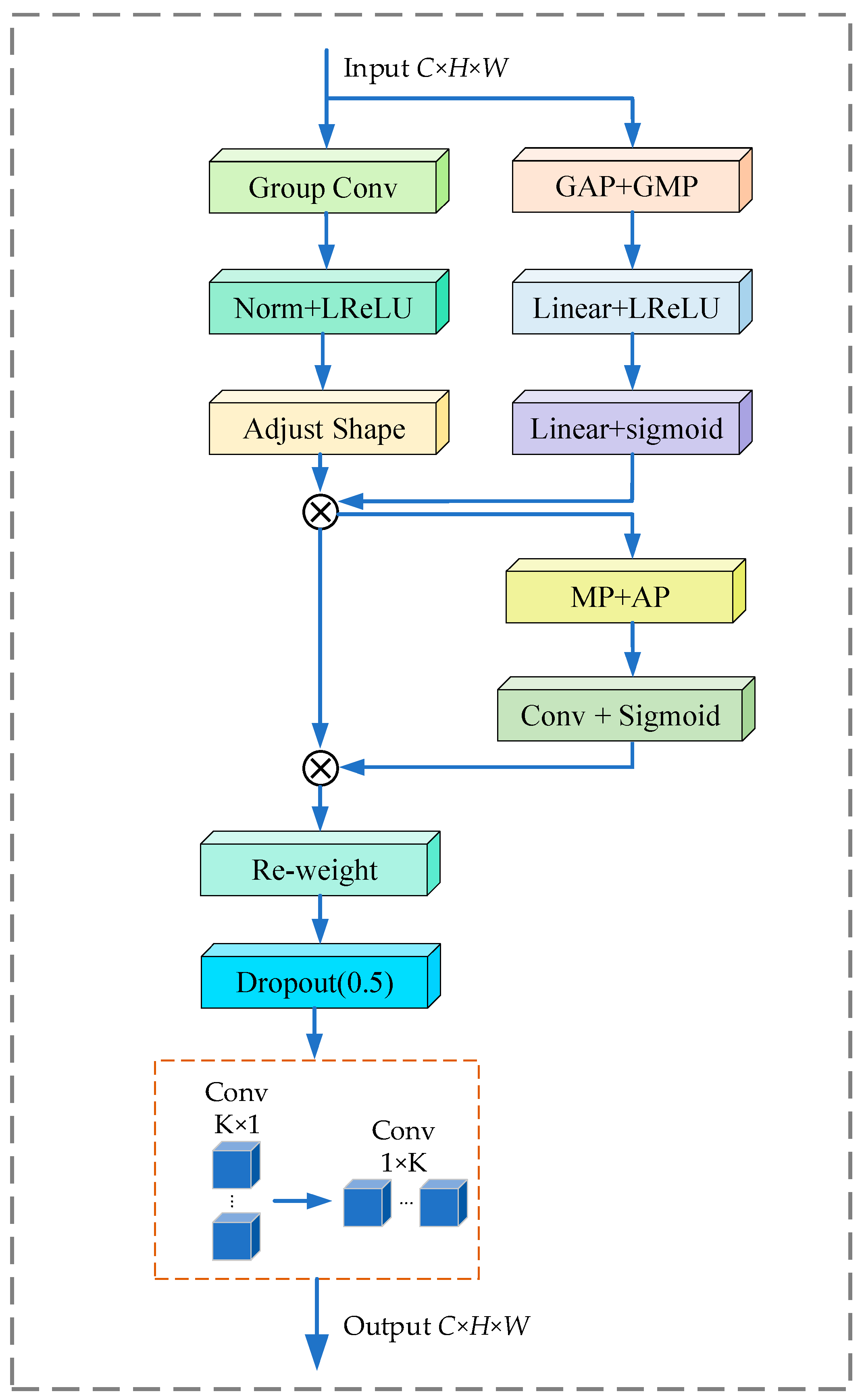
Inspired by RFA, we construct a new modular search space and propose the RFSSA_SepConv operator as shown in Figure 2. C denotes the number of channels in the input. The W denotes the width of the input. H denotes the height of the input. RFSSA_SepConv first extracts the receptive field spatial features using group convolution method. Learning the feature map by interacting with the receptive field feature information can improve the performance of the network. Then, it is normalized by Norm and the LReLu (Leaky ReLu) function, followed by Adjust Shape, in order to adjust the feature shapes. RFSSA_SepConv can completely solve this problem by emphasizing the importance of different features within the receptive field slider and prioritizing the receptive field space features. The feature maps obtained through RFA are sense field space features that do not overlap after “adjust shape”. The learned feature map aggregates the feature information of each receptive field slider. Then, we introduce a spectral attention mechanism and a spatial force mechanism directed to the receptive field features to extract the spectral and spatial information of the HSI. The spectral attention module extracts the spectral global features by both global average pool (GAP) and global max pool (GMP), and passes the obtained features through Linear, LRelu, Linear, and sigmoid activation functions to obtain the spectral weight coefficients. Secondly, the input to the spatial attention module is the result of spectral weighting by HSI, and the spatial attention is max pool and average pool in the channel dimensions, respectively, and then goes through the convolutional layer, and the spatial weight coefficients are obtained by the sigmoid activation function as well. The spatial weight coefficients are subjected to re-weight operation with the spectral weight coefficients to obtain new features. Finally, the standard convolution is decomposed into two steps, depth convolution and point-by-point convolution, by means of the depth-separable convolution module, in order to achieve the purpose of reducing the amount of computation and the number of parameters.
The beginning of the RFSSA_sepConv is a receptive field spatial–spectral attention (RFSSA) module. The end of the RFSSA_sepConv is a depthwise separable convolution module. In the operator, RFA learns the attention graph as non-overlapping receptive field spatial features and summarizes the feature information of each receptive field slider. The method achieves matching spatial attention that focuses on spatial features in the receptive field with convolution, which enhances the advantages of feature extraction and the ability to capture detailed feature information in automatic convolutional neural networks. Meanwhile, it is worth noting that this strategy effectively improves the spatial attention in CBAM, further learns the correlation between the spatial and spectral information of the HSI data, and integrates the information of these two dimensions when performing feature extraction and decision making. Meanwhile, to integrate the global context information into the operator, we employ global average pooling (GAP) to obtain global features of HSI.
In the search for optimal structures, keeping the size of the search space within manageable limits while increasing the likelihood of generating more sub-networks is key to ensuring model diversity and innovation. In addition, the efficiency of searching the search space is crucial. Different convolutions for feature extraction are commonly used operations in NAS-based HSIC tasks, including conventional convolution (CC), separable convolution (SC), and dilated convolution (DC). For different convolutions, the most important issue to consider is the number of parameters. Depthwise separable convolution, as an effective parameter compression technique, significantly reduces the number of parameters in the model, thus helping to reduce computational complexity and storage requirements. In order to simplify the complexity of a single candidate operation and to reduce the burden on the search space, our operators employed depthwise separable (DS) convolution for the extraction of features.
Assume that the input and output of spectral bands are C i n and C o u t , respectively. The parameter P C C of CC is computed as follows:
P C C = C i n × C o u t × K 2
The parameter P D S of DS is expressed as follows:
P D C = C i n × K 2 + C o u t × 1 × 1 × C i n
Taking C i n = C o u t = C , the number of parameters of DS is ( 1 / K 2 + 1 / C ) of CC. Therefore, compared with CC, DS has fewer parameters with the receptive field of the same size.
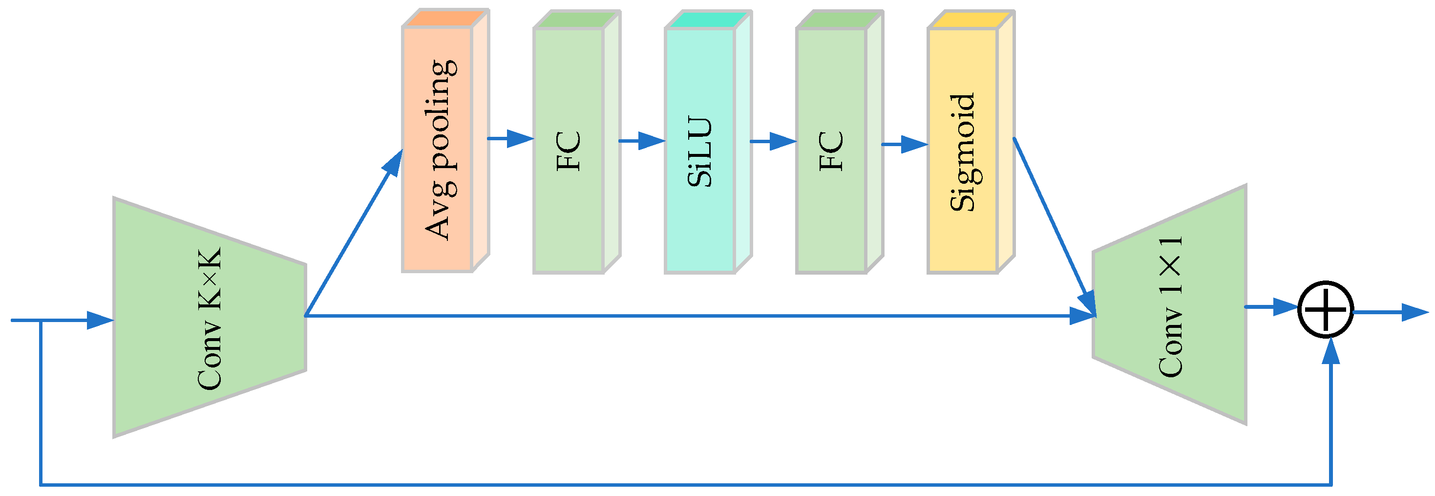
At the same time, considering the requirements of diversity and selectivity of operations within the search space, we successfully introduce Fused_MB convolution [31] as important operators in the search space, as shown in Figure 3. The operator embeds a channel attention module in the convolution layer, which enhances the representation of the network by capturing the interdependencies between feature channels through average pooling operation. This diverse modular search space design not only helps to improve the performance of the model, but may also mitigate the negative impact of shallow inference speed by optimizing feature extraction and attention allocation. During the optimization process, NAS automatically explores the best combinations between operators, thus enriching the selectivity of the model without increasing the burden on the search space. In this way, we are able to search more network structures with excellent performance while maintaining search efficiency.

2.2.2. Search Strategy

As a gradient-based approach, DARTS has become one of the mainstream strategies for neural network structure search. In the search architecture, the architectural parameters a and the network weights w are alternately optimized to minimize the validation loss L v a l ( w , a ) . DARTS employed a bilevel optimization approach to realize the process, shown in Equation (3).
a * = a r g m i n a L v a l ( w * ( a ) , a ) s . t .     w * ( a ) = a r g m i n w L t r a ( w , a )
where L v a l and L t r a denote the validation loss and training loss, respectively.
However, DARTS is largely plagued by the problem of performance collapse due to the aggregation of skip-connections. Specifically, skip-connections form a residual structure that accelerates the flow of information when summed with other candidate operations. Skip-connections benefit overly from the unfair competitive advantage, resulting in searched models that tend to have an excessive number of skip-connections appearing, drastically reducing search performance. To weaken the impact, the unfair competitive advantage of skip-connections is reduced by injecting unbiased noise into the skip-connections to impede the flow. Therefore, in the paper, Noisy-DARTS [32] is employed to search the network architecture. We add noise after skip-connections to disrupt the gradient flow and allow all candidate operations to compete on a fair field. The search process is displayed in Figure 4 where different colored arrows indicate different candidate operations.
In Noisy-DARTS, we add unbiased Gaussian noise x ˜ ~ N ( μ , σ ) (taken μ = 0 , σ = 0.2 ) into skip-connections to diminish the benefits of the residual structure and address the performance collapse. The loss function of a skip-connection can be written as
L = L v a l ( y * ) ,   y * = f ( a s k i p ) ( x + x ˜ )
where a s k i p is the corresponding architectural weight of skip-connection and f ( a s k i p ) is the softmax output for a s k i p . When the Gaussian noise is much smaller than the output feature, we get Equation (5).
y * f ( a s k i p ) · x   when   x ˜ < < x
After adding the noise, the gradient of the parameters of the skip-connection is shown in Equation (6).
L a s k i p = L y * y * a s k i p = L y * f ( a s k i p ) a s k i p ( x + x ˜ )
Based on the analysis, assuming x ˜ < < x , injection of noise does not affect the normal gradient update during the architecture search. Therefore, the unbiased Gaussian noise is used to balance the unfair competition. The Noisy-DARTS injects the Gaussian noise x ˜ into skip-connection to obtain Equation (7).
o ¯ i , j = k = 1 S - 1 f ( a o k ) o k ( x ) + f ( a o s k i p ) o s k i p ( x + x ˜ )
where n i is a node in cell and o i , j ( x i ) is an output feature operation set between n i and n j . O = { o i , j 0 , o i , j 1 , , o i , j S 1 } was denoted as S candidate operations on e i , j . o i , j s k i p was denoted as the skip-connection between n i and n j x ˜ introduces uncertainty into the gradient update, and the skip-connections need to overcome the uncertainty to compete with other operators. As a result, the unfair advantage is effectively minimized, thus creating a fair competition environment.

2.2.3. Performance Evaluation Strategy

The number of samples of multiple categories in the HSI dataset exhibits a long-tailed distribution, which brings about the problem of category imbalance; i.e., the number of samples of certain categories is small, which leads to difficulties in classifying these categories. In classification tasks, the commonly used cross-entropy loss function focuses on learning information between categories. However, the category imbalance problem and classification boundary blurring problem of HSI data lead to the dispersion of features learnt by the cross-entropy loss function. Therefore, we introduce PL [33] on top of SM and construct a fusion loss function to deal with the category imbalance problem.
PL approximates the commonly used efficient loss functions by Taylor expansion, which designs the loss function as a linear combination of polynomials. In the paper, PL skillfully decomposes loss function into a series of weighted polynomial bases, each corresponding to a set of polynomial coefficients. By adjusting the weights of these polynomial bases, the model is made to pay more attention to hard-to-classify samples during training, thus achieving higher classification performance. The experimental results show that the loss function based on multiple categories has excellent results and helps to alleviate the category imbalance problem.
L P L = ( 1 P t ) γ log ( P t ) + j = 1 N ε j ( 1 P t ) j + γ
where j denotes the power of the polynomial basis. γ denotes the power shift of the polynomial term. P t denotes predicted probability for samples. ε j [ 1 / j , ) denotes the perturbation term that allows us to determine the first N polynomials while ignoring the coefficients of multiple higher-order ( j > N + 1 ). In Formula (8), tuning the first polynomial often yields the most significant gains. Thus, PL can be further simplified as shown in Formula (9).
L P L = 1 P t γ log P t + ε 1 1 P t 1 + γ
Label smoothing, as a regularization technique, can effectively help models generalize better, prevent overfitting, and improve model correction, which is expressed as follows:
L SM = i = 1 K y i log q i
y i = ( 1 θ ) ,   if   ( i = y ) ( θ K 1 ) ,   if   ( i y )
q i = exp ( x i ) j = 1 K exp ( x j )
where θ denotes hyperparameters and is set to 0.05. y is the label of x with K categories. y i is the probability of each category of label.
We combine PL with SM to construct an efficient fusion loss function. When confronted with the problem of class imbalance, we can increase the loss weights of the unbalanced categories, thus improving the ability of the model to recognize these categories.
L P M = L P L + L S M
The overall algorithm flow of the proposed RFSS-NAS is written as Algorithm 1.
Algorithm 1
Input: Training set ( X t r a , Y t r a ) ,   validation   set   ( X v a l , Y v a l ) ,   test   set   ( X t e s t , Y t e s t )
Initialization: Defining the search space (including candidate operation set O ), construct supernet S (network weights W = { w ( i , j ) }   and   architecture   parameters   A = { α ( i , j ) } ), noise standard variance σ , batch size = 32, epochs = 100.
Search Stage:
     While reach epochs do
         1. Inject Gaussian noise x ˜ into the output of skip-connections
         2. Input   training   set   and   compute   L t r a
         3. Update the weight w   by   compute   w L t r a ( w , a )
         4. Input   validation   set   and   compute   L v a l
         5. Fix w and update the architecture parameters α   by   compute   α L v a l ( w , α )
     End while
Deducing the Final Network: Derive sub-network consisting of the operations with the highest weights at each layer is selected as the final network according to learned α .
Final Network: Input training set and validation set to train the final network and optimizes weighs w .
Classification Stage:
     for sample in  X t e s t :
          Output the predicted results.
Obtain classification results.

3. Results

In this section, we designed a series of related experiments on three public datasets to validate the performance of the proposed RFSS-NAS. First, we described the datasets and experimental setup in detail. Second, for the purpose of evaluating the validity, we compared the RFSS-NAS with classification methods of HSI. Finally, to showcase the comprehensive RFSS-NAS, we provided the exhaustive visualization results and a detailed dissection.

3.1. Datasets Description

In the process of performing our experiments and analyses, three available HSI datasets are employed to evaluate the RFSS-NAS, including the Kennedy Space Center (KSC), Pavia University (PU), and Houston (HU) datasets. Among them, the PU and HU datasets cover complex and varied urban scenarios with rich and diverse data characteristics, which provide researchers with challenging experimental environments. Especially in the small sample classification task, due to the limited number of samples and subtle features, the accuracy and robustness of the classification algorithms are more demanding.
  • The KSC dataset was taken by the AVIRIS sensor at the Kennedy Space Center in Florida in 1996. There are 224 bands in the raw data, and, after removing the water vapor noise and low signal-to-noise bands, 176 bands remained for the experiments. The spectral range is 0.4–2.5 µm and the spatial resolution is 18 m with 13 categories. The KSC dataset labeled sample information is described in Table 2.
2.
The PU dataset was gathered on the campus map of the Pavia University in northern Italy in 2003. The spatial resolution is 1.3 m size of 610 × 340 pixels. It covers nine different urban categories, totaling 42,776 samples and retaining 103 spectral bands, with a spectral region of 0.43–0.86 µm. The PU dataset labeled sample information is described in Table 3.
3.
The HU dataset was acquired in 2013 by the ITRES CASI-1500 sensor, which covered the University of Houston campus and surrounding urban land area. The spatial dimension is 329 × 1905 pixels with spatial resolution of 2.5 m. It contains a total of 54,129 samples, covering 15 land cover categories and retaining 144 spectral bands for research with a spectral region of 0.36–1.05 µm. The HU dataset labeled sample information is described in Table 4.

3.2. Implementation Details

To comprehensively and objectively evaluate the performance of different methods in the HSIC task, we combined both quantitative and qualitative analyses to provide an in-depth and detailed assessment of the various methods. For the quantitative assessment, the study used three metrics, including overall accuracy (OA), average accuracy (AA), and Kappa coefficient (K). Table 5 reported the information of the training and validation samples.
All the experiments are conducted under the computer configuration as follow: an Intel (R) Xeon (R) CPU E5-2620 v4 @ 2.10 GHz, 128 GB RAM (Intel Corporation, Santa Clara, CA, USA), and an NVIDIA GeForce 2080 Ti graphical processing unit (GPU) (Nvidia Corporation, Santa Clara, CA, USA). The software environment is the system of 64-bit Windows 10 with open-source framework Pytorch 1.12.1. The Adam optimizer is used to optimize the architecture parameters with the default weight decay = 0.0003, the learning rate = 0.004, the grad clip = 5, the drop prob = 0.2, and the momentum = 0.9.
For the purpose of verifying the classification accuracy under the condition of limited training samples, we adopt a well-designed sample division strategy. First, 30 samples of each class are randomly selected as the training set, another 10 samples are selected as the validation set for model parameter tuning and performance evaluation, and the remaining samples form the test set. Meanwhile, to ensure a fair and stable comparison, all experimental results were averaged after ten repetitions as the final result. To adapt to the hardware resource limitation and reduce the computational load of network training, we set the batch size of both training and validation to 32. In the search phase of the supernet architecture, we set the search epochs to 100. The experimental results show that all the experimental networks are able to reach a stable convergence state after 200 epochs of training. Therefore, to ensure that the final network is fully optimized, we extend the training epochs to 500 to fully exploit the potential of the network and improve the model performance.

3.3. Comparison of the Proposed RFSS-NAS with the State-of-the-Art Methods

In this section, we focus on comparing the proposed RFSS-NAS with the traditional methods, and CNN-based and NAS-based methods, including the radial basis function support vector machine (RBF-SVM) [34] and CNN [35], pyramidal residual networks (PyResNet) [36], spectral–spatial residual network (SSRN) and NAS-based automatic design of convolutional neural network (3-D AT-CNN) [24], hybrid neural architecture search (HNAS) [37], and lightweight multiscale neural architecture search (LMSS-NAS) [26].

3.3.1. Quantitative Analysis

Table 6, Table 7 and Table 8 reported the quantitative experimental results of various methods on different datasets. Clearly, the proposed RFSS-NAS consistently outperforms other comparative methods in terms of evaluation metrics, which shows that RFSS-NAS effectively avoids the biases of manual design by using automated architectural search and delivers an optimized resource-efficient model.
Specifically, for the KSC dataset, especially on the fifth class of samples, the OA of RBF-SVM and CNN are only 60.22% and 38.73%. We attribute this phenomenon to the unique challenges posed by the sparser sample distribution of the KSC dataset. However, 3-D AT-CNN (97.46%), HNAS (96.46%), LMSS-NAS (97.40%), and RFSS-NAS (97.90%) generally demonstrated a superior performance on the fifth category. Meanwhile, the OA of RFSS-NAS is comparable to LMSS-NAS, which further illustrates the greater adaptability of NAS-based methods to categories with complex feature distributions. On the PU dataset, RFSS-NAS obtains a superior OA of 98.79%. Compared to other NAS-based approaches, RFSS-NAS improves +3.97% (3-D AT-CNN), +3.48% (HNAS), and +2.45% (LMSS-NAS), respectively. The HU dataset covers more categories and has a more discrete distribution of the same categories, which creates challenges for small sample classification tasks. With 30 training samples taken from each category, RFSS-NAS achieves an OA of 96.91%, while the handcrafted models of RBF-SVM, CNN, PyResNet, and SSRN reach 76.15%, 93.55%, 91.29%, and 94.69%, respectively. For NAS-based methods, 3-D AT-CNN, HNAS, and LMSS-NAS achieve 89.59%, 88.40%, and 93.07% in terms of OA.
After a careful evaluation of the experimental results, it can be understood that the NAS-based approach outperforms the handcrafted approach in terms of overall performance, which clearly showcases that NAS has a greater adaptability to various HSI datasets. In addition, from the perspective of models based on spectral–spatial information, the methods equipped with attention mechanisms, such as HNAS, LMSS-NAS, and RFSS-NAS, have demonstrated superior overall classification accuracy compared to those without attention mechanisms, such as CNN, PyResNet, RSSN, and 3-D AT-CNN. This observation underscores the significance of incorporating attention mechanisms in spectral–spatial analysis, enabling the models to focus on salient features and enhance classification performance. Meanwhile, from the perspective of NAS methods that also incorporate attention mechanisms, LMSS-NAS and RFSS-NAS demonstrate a superior performance compared to HNAS. This observation suggests that the modular design that combines attention with convolution within NAS methods is more advantageous for spatial–spectral feature extraction than treating attention as a standalone operator. Our proposed RFSS-NAS exhibits optimal overall performance, primarily due to the RFSSA_SepConv, which not only focuses on critical features but also possesses the capability to extract long-range information. Furthermore, RFSS-NAS employs the Noisy-DARTS search strategy to address the issue of unfair competition, thereby preventing significant performance losses in the final model, ensuring a more balanced and optimal search process to improve the classification accuracy and stability.

3.3.2. Qualitative Analysis

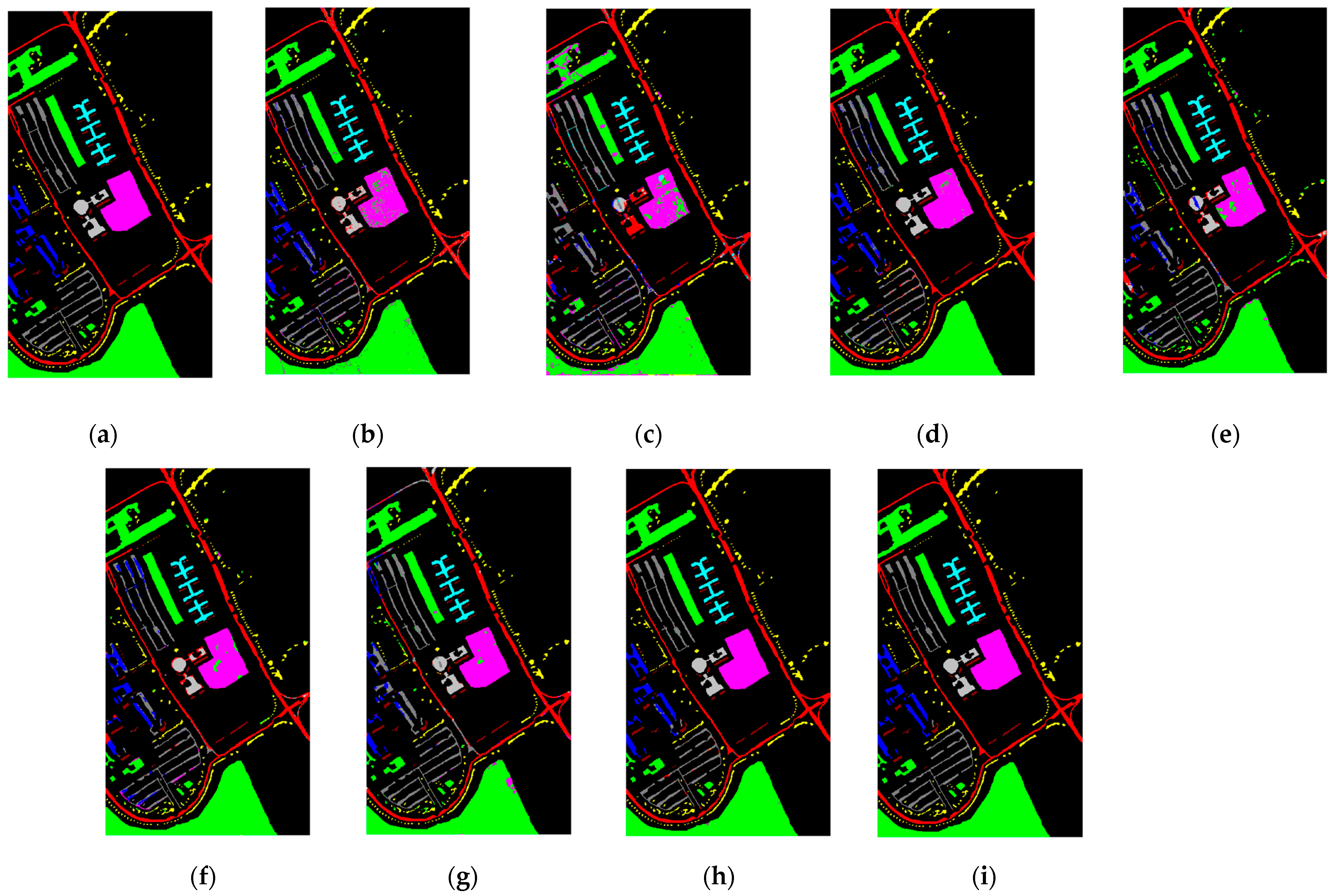
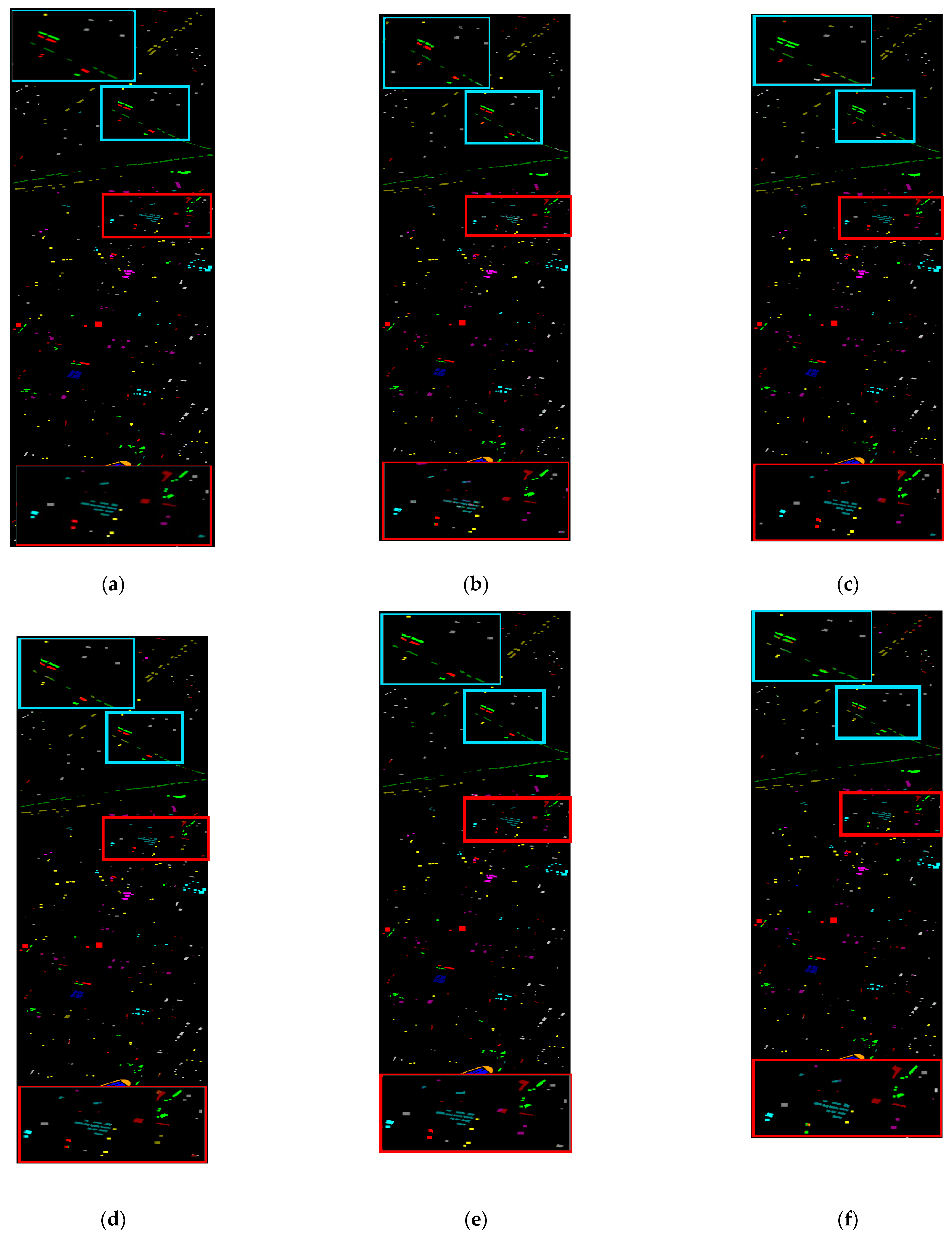
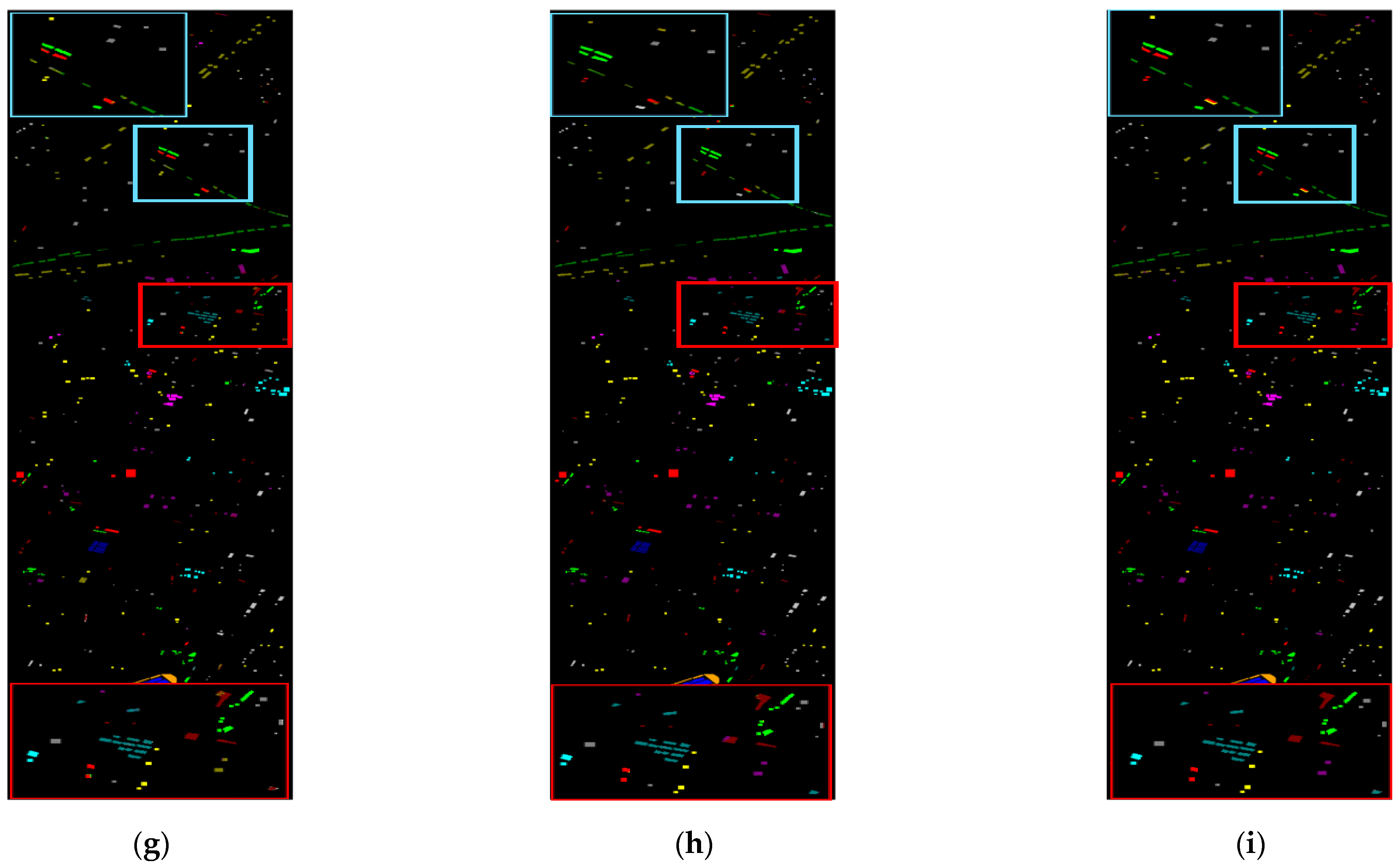
Figure 5, Figure 6 and Figure 7 show the classification visual effects of eight different classification methods on the KSC, PU, and HU datasets, respectively. Compared with the classification maps of other methods, our proposed classification method is the closest to the real ground truth. On the PU dataset, it can be clearly seen that the RBF-SVM CNN method has a very obvious classification error on the Bare Soil category, which is misclassified as the Meadows category, and there is a lot of noise scattering in the other classification methods, and, in analyzing a large area of the same kind of area, the proposed method effectively reduces the noise and misclassified area, showing a smoother categorization effect, which reflects the spatial continuity. On the KSC dataset and HU dataset, compared with the truth map, it can be seen that the classification effect of the proposed method has a higher classification accuracy in recognizing relatively scattered and complex features.

4. Discussion

4.1. Optimal Architecture Analysis

Figure 8, Figure 9 and Figure 10 displayed the optimal architectural units obtained through our proposed approach. In the experiments, we adopted the Noisy-DARTS search strategy to precisely find the optimal cell architecture for different datasets in a specific supernet. It is clear from the following figures that the cell architecture connections and operations searched for each dataset exhibit uniqueness. This is precisely because the Noisy-DARTS search strategy is able to adaptively select the cell structure that best matches the characteristics of different datasets. On the KSC dataset, the normal cell exhibits a balanced choice between convolution and pooling operations, reflecting the algorithm’s comprehensive consideration of different features in the dataset. On the PU and HU datasets, the normal cell prefers the convolution operation to dig deeper into the discriminative features in the dataset. This difference in cell structure not only reflects the adaptability of RFSS-NAS to different datasets, but also demonstrates its flexibility in handling different tasks.

4.2. Search Space Validity Analysis

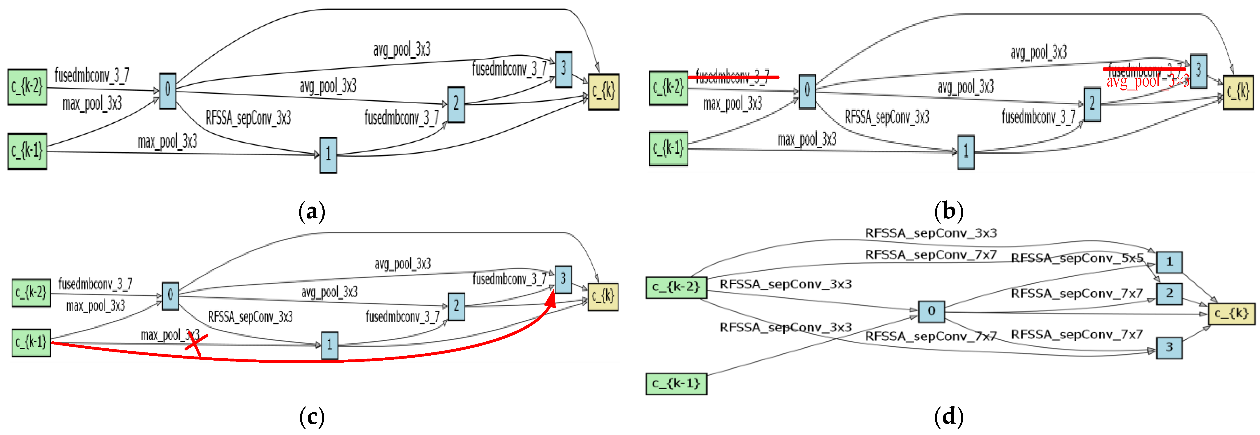
In the RFSS-NAS method, the cell structure is based on the combination of candidate operations in the search space. By finely searching the optimal combinations between candidate operations, the adaptive learning of HSI features can be efficiently realized to perform high-precision classification tasks. Therefore, to verify the reasonableness and effectiveness of the final unit structure, we manually modify the searched final architecture in different ways to verify whether RFSS-NAS has truly found an efficient architecture through the search, rather than simply integrating various convolutions and branches to improve the performance.
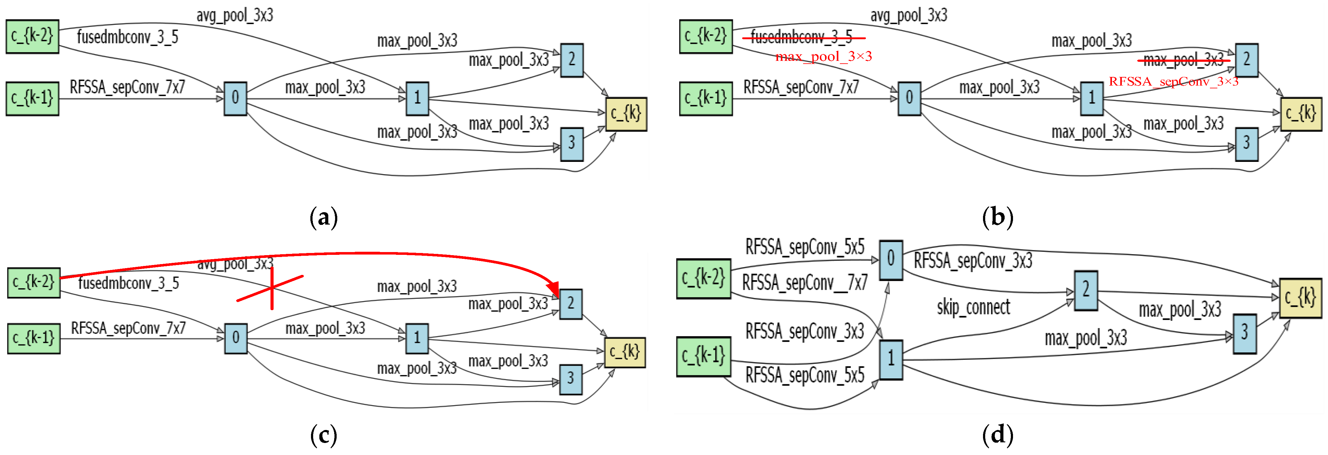
Specifically, the modifications are: (1) randomly replacing selected operations with candidate operations in the search space (called RFSS-NAS-Rop); (2) changing the connectivity between nodes in the cell (called RFSS-NAS-Rtopo); and (3) performing HSIC tasks on the KSC dataset with the final architecture of the HU dataset (called RFSS-NAS- Rob). Following the above three modifications, we have modified the structure of the searched cells using the KSC dataset as an example, and its modified structure is shown in Figure 11 and Figure 12.
Based on the analysis of the experimental results, we found that the performance derived from the modified structure is lower than the final architecture automatically searched out. The results are listed in Table 9, from which the following conclusions can be drawn: (1) RFSS-NAS can select the optimal operation for each node. Comparing RFSS-NAS and RFSS-NAS-Rop, the performance of the architecture after randomly replacing the operations is lower than that of the automatically searched out architecture. (2) The final architecture searched out by RFSS-NAS has the capability of efficient topology. The modification in topology decreases the evaluation metric AA to 98.63%. (3) Changing the node connections of the network architecture has a greater impact on the classification accuracy than randomly replacing the selected operations. (4) RFSS-NAS is able to search for the respective optimal architecture based on the characteristics of different datasets. Comparing RFSS-NAS and RFSS-NAS-Rbop, the architecture of RFSS-NAS with HU has decreased the classification accuracy on the KSC dataset.
Overall, the experiments fully validate the effectiveness of RFSS-NAS in searching for neural network architectures, which search for optimal structures that are not the result of random integration operations. Any minor adjustments to the final architecture resulted in performance degradation, proving its local optimality in the search space.

4.3. The T-Distributed Stochastic Neighbor Embedding Analysis

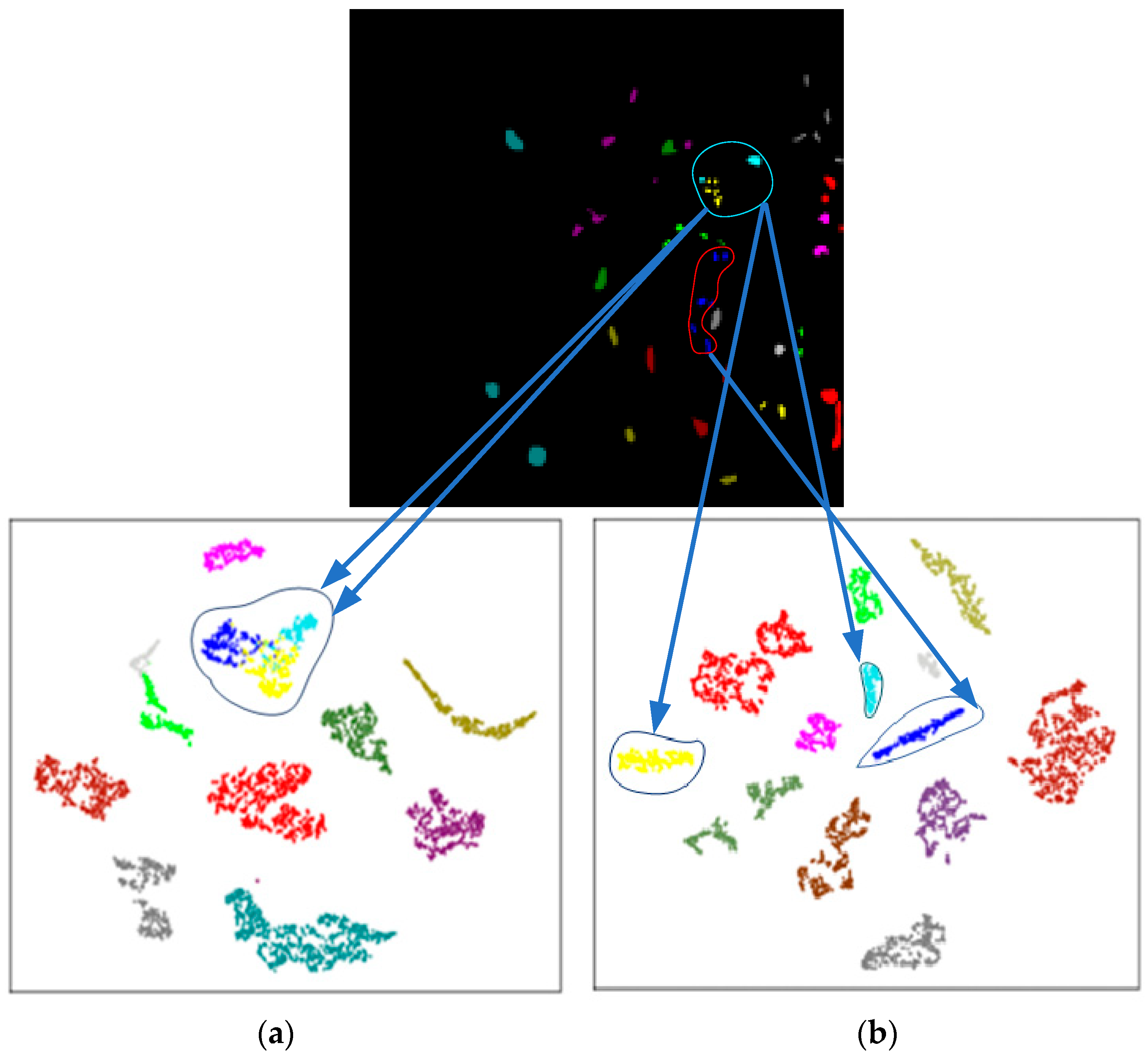
To verify the superiority of RFSSA in terms of model performance, we deeply explored the data distribution characteristics of the labeled samples on the KSC dataset. With the help of 2D t-distributed stochastic neighbor embedding (t-SNE) visualization technique, we obtained the results as displayed in Figure 13. Without applying RSSFA, the heterogeneous labels in the feature space are highly confounded. However, when RSSFA is added, the sample distribution becomes significantly more compact and the data point clustering is significantly improved with more distinct boundaries. This significant change fully demonstrates the power of RFSSA in extracting and representing spatial–spectral features, and its ability to effectively learn and abstract feature information that is essential to the HSIC task. Therefore, we have reason to believe that the introduction of RFSSA will greatly enhance the classification accuracy and stability of the model.

4.4. Confusion Matrix

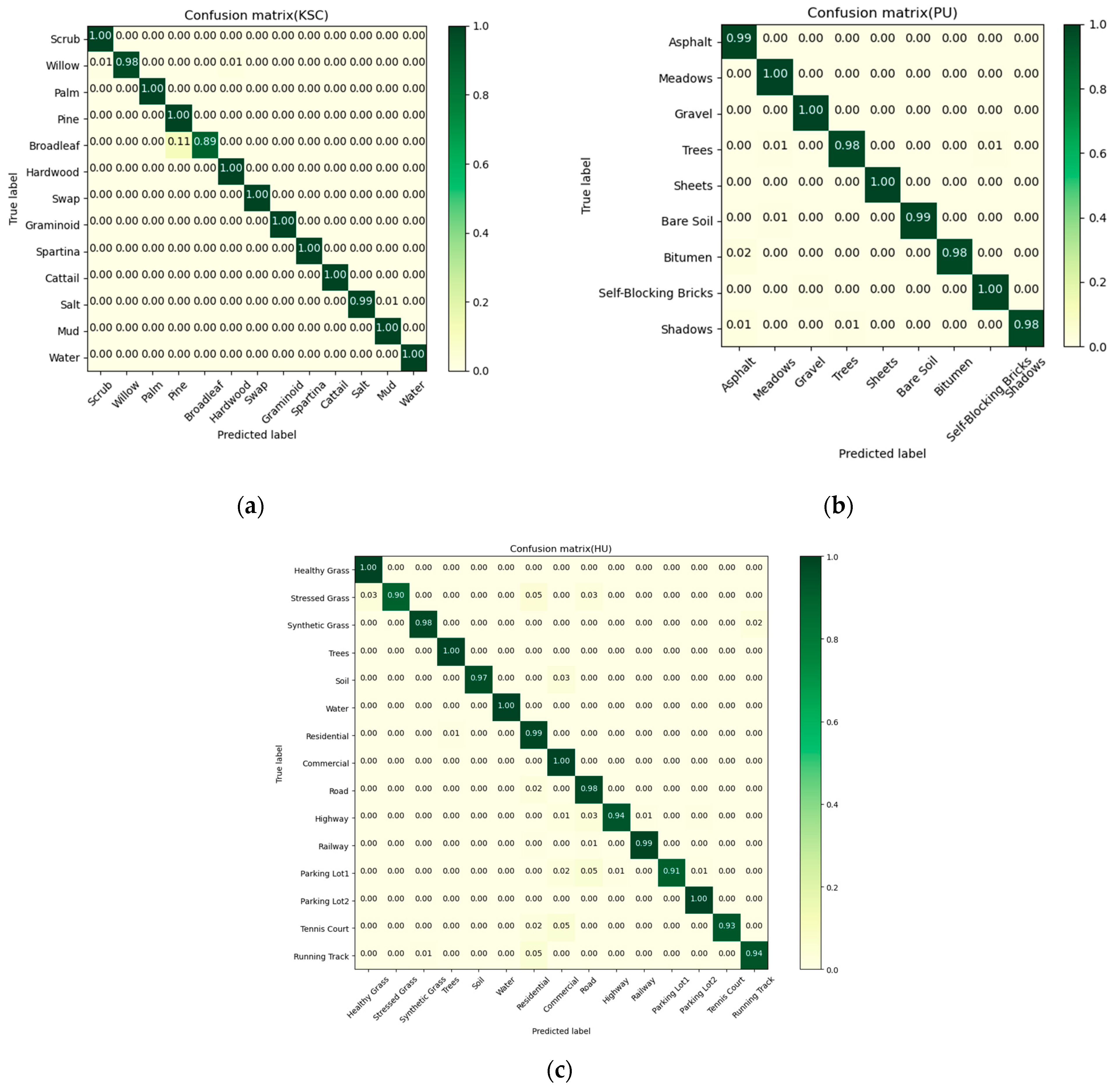
For the purpose of more intuitively displaying the HSIC efficacy of RFSS-NAS, we specifically plotted the confusion matrices on the KSC, PU, and HU datasets, as shown in Figure 14. For both the KSC and PU datasets, the high degree of matching between the predicted and true labels of the classification results demonstrates the ability of RFSS-NAS to robustly and accurately classify different land feature categories. However, on the HU dataset, due to the complex distribution of features, RFSS-NAS performs slightly poorly on some hard-to-recognize categories such as Stressed Grass, Highway, etc. Nonetheless, RFSS-NAS can still achieve a satisfactory classification accuracy with its ability to capture a larger range of homogeneity as well as the error reduction mechanism. Overall, RFSS-NAS demonstrates stable classification performance on multiple datasets.

4.5. Ablation Experiments and Dada Imbalance Analysis

To evaluate the gain effects of Fused_MBConv, RFSSA_SepConv, and Noisy-DARTS, we designed ablation experiments on the PU dataset. The results are exhibited in Table 10. The results of the ablation experiments show that the absence of any of the modules in the model leads to performance degradation. Only when all three modules are retained intact, the final network obtained through the search can achieve optimal classification. Among these, compared to the combination of Fused + Noisy-DARTS (96.36%), the combination of RFSSA + Noisy-DARTS (98.20%) improves by +1.84%, which proves that the RFSSA has a stronger performance in the extraction of discriminative features. Moreover, when Noisy-DARTS is adopted as the search strategy, the performance of the final network searched is further optimized, which fully proves that Noisy-DARTS robustly creates a level playing field for the search environment and effectively mitigates the performance crash during the search process. This finding emphasizes the critical effect of synergy among modules in improving model performance, further highlighting the rationality and necessity of model design.
Due to the long-tailed distribution of the HSI data, there will exist a sample imbalance problem. Therefore, we introduced PL to construct a fusion loss function based on SM. The core idea of the PL function is to assign more attention to categories with fewer samples by adjusting the polynomial coefficients. In order to verify the performance of this loss function, we conducted ablation experiments on three datasets, and the results are shown in Table 11.
It can be seen that PL has a positive effect on all three datasets. The use of PL improves OA by 0.47–1.70%, AA by 0.78–1.13%, and Kappa by 0.62–1.51%. Meanwhile, we noticed that PL significantly improves AA, which proves that PL effectively improves the accuracy of single-class categorization and mitigates the sample imbalance problem. These quantitative results tabulate that the loss function favorably contributes to the HSIC results, especially for the unbalanced sample classification task. The method further improves the classification accuracy mainly by weighting the loss function to speed up the model convergence, decreasing the intra-class distance and increasing the inter-class distance, and emphasizing the categories that are prone to misclassification.
Combined with the results in Table 8, although RFSS-NAS achieves a good classification accuracy on OA, AA and most of the classes, the accuracy of category 14 (Tennis Court) performs a little poorly. Based on the analysis of the results in Figure 14c, we can see that a few edge samples in category 14 by having 0.05% and 0.02% are misclassified as category 8 (Commercial) and category 7 (Residentail), respectively. The main reason for this is their similar spatial–spectral features, which leads to the misclassification of edge samples in category 14. Although RFSS-NAS performs poorly in some hard-to-classify categories, it still achieves a good overall classification accuracy due to its ability to capture a larger range of homogeneity and reduce misclassification.

4.6. Convergence Experiment and Correlative Parameter Analysis

Table 12 presents the resource cost of 3D-CNN, PyResNet, SSRN, 3-D AT-CNN, HNAS, LMSS-NAS, and RFSS-NAS, including the parameters, training time, and test time. Compared to 3-D AT-CNN, RFSS-NAS employs more efficient and complex modules, and, therefore, searches an increased number of parameters in the final architecture. However, it is worth noting that RFSS-NAS has a significant advantage in classification accuracy. This advantage compensates for the shortcomings of RFSS-NAS in terms of resource consumption. Considering that classification performance is a critical metric in practical applications, RFSS-NAS’s balance between performance and efficiency is reasonable. Meanwhile, compared with PyResNet and HNAS, RFSS-NAS has obvious advantages in both efficiency and performance. This excellent performance demonstrates that RFSS-NAS is able to achieve superior classification performance at moderate computational cost, providing an effective and feasible solution for automatically generating optimal architectures for HSI classification tasks.
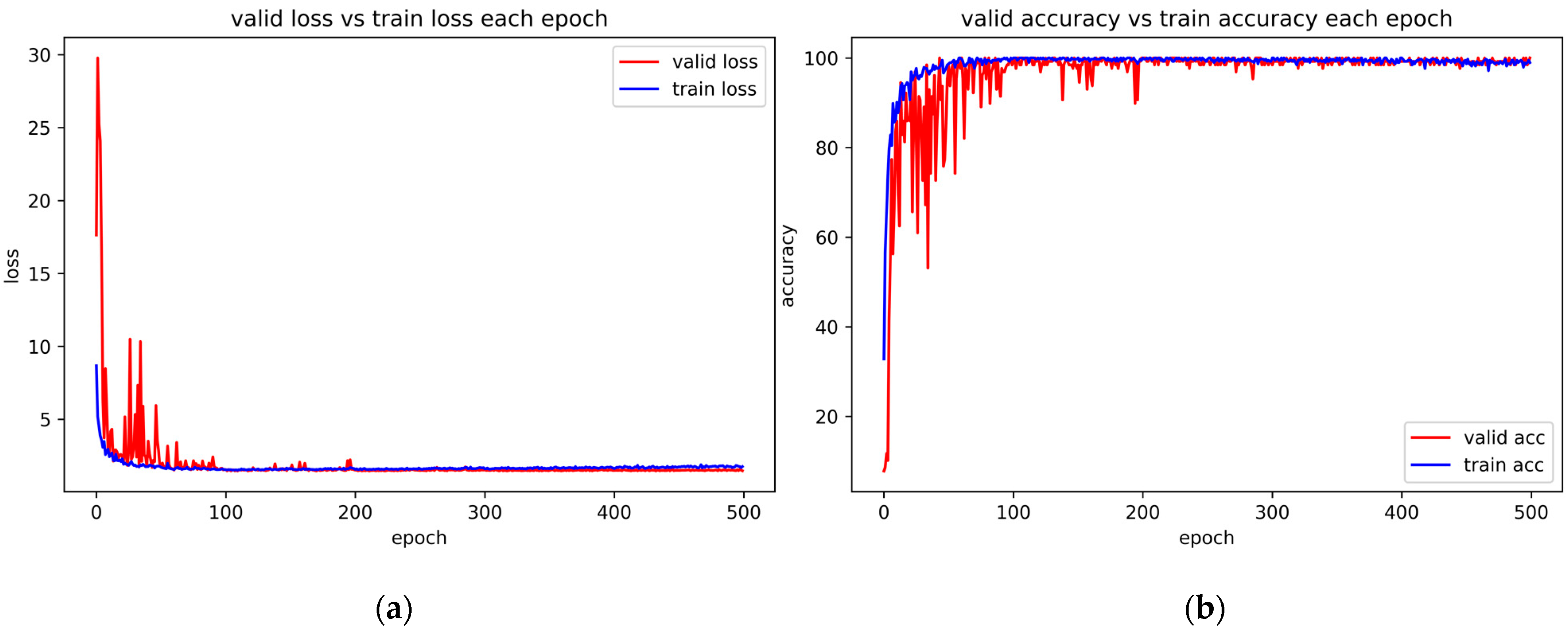
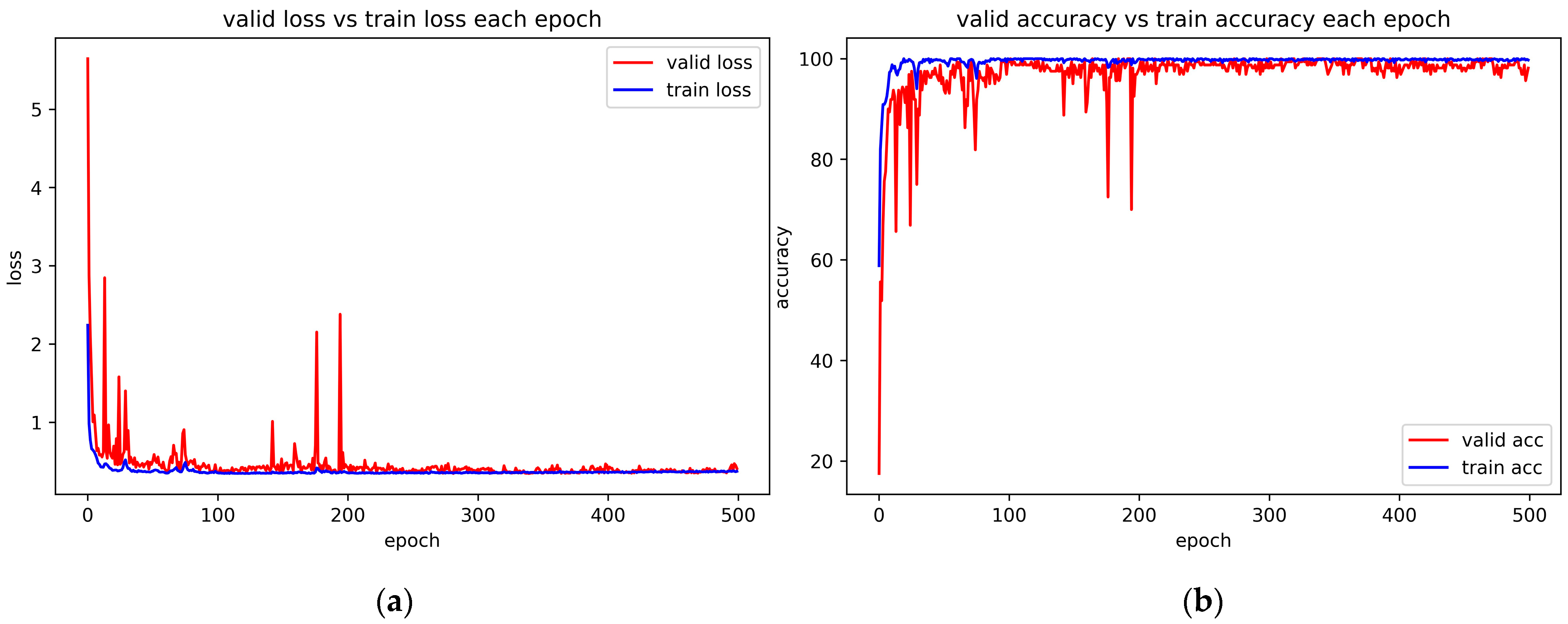
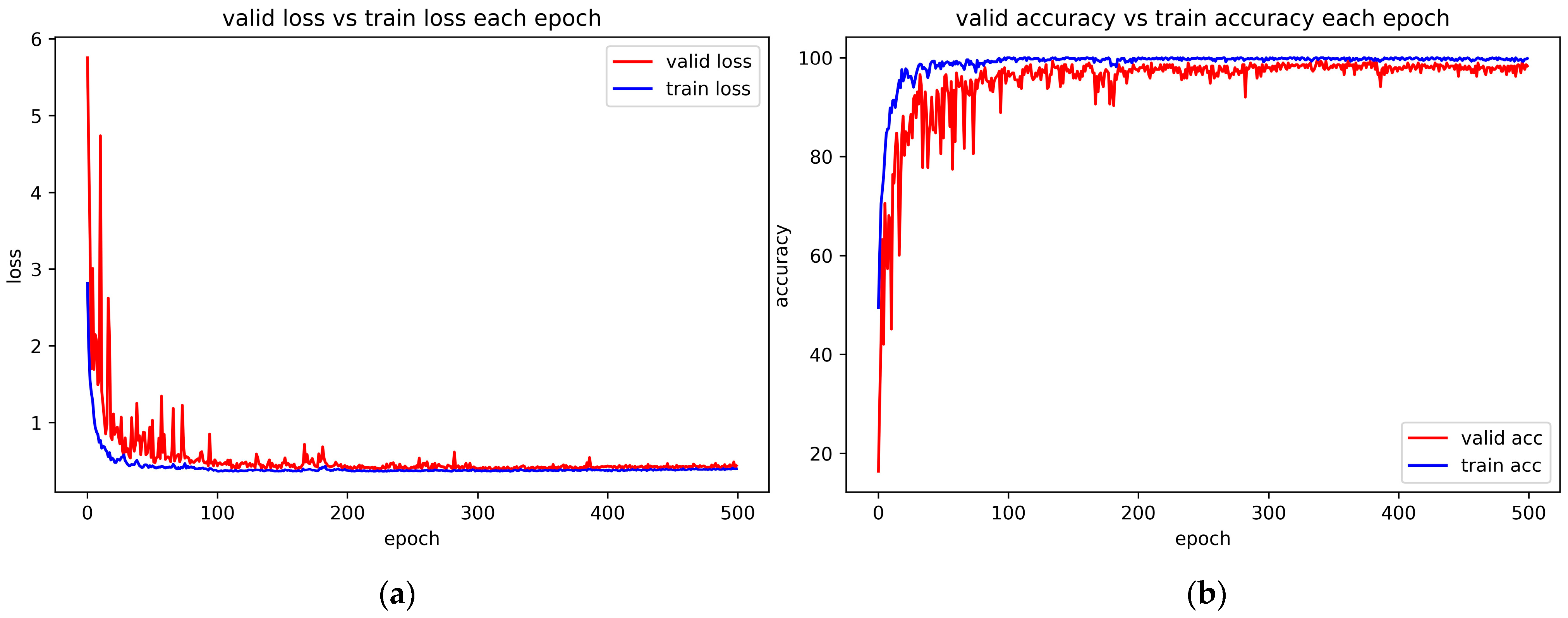
We conducted convergence experiments on the loss and accuracy of training and testing on the three data sets, respectively, as shown in Figure 15, Figure 16 and Figure 17. As can be seen from Figure 15a, Figure 16a and Figure 17a, with the increase in the epoch, the loss of the training set and verification set on the KSC dataset, PU dataset, and HU dataset gradually decreases, and becomes stable at epoch 200, and the loss of the training set and verification set is close to each other and the loss value is low. The model learned the data well, and there were no obvious overfitting and underfitting phenomena. As can be seen from Figure 15b, Figure 16b and Figure 17b, the accuracy curves of the training set and the verification set begin to show an obvious and rapid upward trend, indicating that the model is effectively learning data. At the epoch of 200, the accuracy curves of the training set and the test set continue to stabilize and converge well.
In order to test the effect of different noises on the performance of RFSS-NAS, we compare the effectiveness of Gaussian noise and uniform noise in Table 13. From the analysis of the experimental results, both of them improve the performance of RFSS-NAS, while the gain effect of Gaussian noise is better than that of uniform noise.
In order to verify the effect of training samples on the experimental accuracy, we used different proportions of training samples for the experimental analysis. Taking the PU dataset as an example as shown in Table 14, we tested the classification performance of RFSS-NAS on small samples using sample proportions of 0.10%, 0.21%, 0.31%, 0.42%, 0.53%, and 0.63%, respectively. It can be seen that the classification performance gradually improves as the sample proportion increases. It is noteworthy that, when only 0.53% of the training samples is used, the OA of RFSS-NAS exceeds 93% on all three datasets.

5. Conclusions

In the paper, a novel RFSS-NAS is innovatively designed based on the neural architecture search approach, providing an efficient and automated design solution for HSIC. Specifically, this study combines the attention mechanism to create an efficient receptive field spatial–spectral attention separable convolution operator to construct the search space. The operator integrates the RFA to deeply excavate more discriminative features, which significantly improves the ability of feature differentiation among different land covers. In response to the performance collapse problem of traditional DARTS due to unfair competition during the search process, we successfully balance the competition among candidate operations by injecting Gaussian noise into skip-connections, ensuring the consistency of the search and evaluation process. In the performance evaluation session, we combine the label smoothing loss function with the polynomial expansion perspective loss function to construct a fusion loss function, which effectively alleviates the HSI inter-class imbalance problem and further improves the classification accuracy. Moreover, we verified that RFSS-NAS indeed finds efficient topologies and chooses optimal operations, rather than simply integrating branches and various convolutions to form a network. The experimental results show that our proposed RFSS-NAS exhibits excellent competitive advantages for HSIC.
The performance of the NAS-based HSIC method is mainly limited by the design of candidate operations within the search space, as well as the limited size of the search space. In future, we will aim to explore larger-scale search spaces to increase the number of possible architectures. In addition, most of the current NAS-based HSIC classification methods are performed in supervised scenarios, which limits their application scope to some extent. Therefore, our next goal is to explore semi-supervised methods to expand the applicability and usefulness of NAS.

Author Contributions

Conceptualization, A.W., K.Z., S.D., H.W., Y.I. and X.Y.; methodology, K.Z. and S.D.; software K.Z. and S.D.; validation K.Z.; writing—review and editing A.W., K.Z., S.D., H.W., Y.I. and X.Y. All authors have read and agreed to the published version of the manuscript.

Funding

This work was funded by the Key Research and Development Plan Project of Heilongjiang (JD2023SJ19), the Natural Science Foundation of Heilongjiang Province (LH2023F034), the High-End Foreign Experts Introduction Program (G2022012010L), the Key Research and Development Program Guidance Project of Heilongjiang (GZ20220123) and the Science and Technology Project of Heilongjiang Provincial Department of Transportation (HJK2024B002).

Data Availability Statement

Conflicts of Interest

The authors declare no conflicts of interest.

References

  1. Ghamisi, P.; Maggiori, E.; Li, S.; Souza, R.; Tarablaka, Y.; Moser, G.; Giorgi, A.D.; Fang, L.; Chen, Y.; Chi, M.; et al. New frontiers in spectral-spatial hyperspectral image classification: The latest advances based on mathematical morphology, Markov random fields, segmentation, sparse representation, and deep learning. IEEE Geosci. Remote Sens. Mag. 2018, 6, 10–43. [Google Scholar] [CrossRef]
  2. Della, C.; Bekit, A.; Lampe, B.; Chang, C.-I. Hyperspectral image classification via compressive sensing. IEEE Trans. Geosci. Remote Sens. 2019, 57, 8290–8303. [Google Scholar] [CrossRef]
  3. Hestir, E.; Brando, V.; Bresciani, M.; Giardino, C.; Matta, E.; Villa, P.; Dekker, A. Measuring freshwater aquatic ecosystems: The need for a hyperspectral global mapping satellite mission. Remote Sens. Environ. 2015, 167, 181–195. [Google Scholar] [CrossRef]
  4. Shimoni, M.; Haelterman, R.; Perneel, C. Hypersectral imaging for military and security applications: Combining myriad processing and sensing techniques. IEEE Geosci. Remote Sens. Mag. 2019, 7, 101–117. [Google Scholar] [CrossRef]
  5. Lu, G.; Fei, B. Medical hyperspectral imaging: A review. J. Biomed. Opt. 2014, 19, 010901. [Google Scholar] [CrossRef] [PubMed]
  6. Murphy, R.; Schneider, S.; Monteiro, S. Consistency of measurements of wavelength position from hyperspectral imagery: Use of the ferric iron crystal field absorption at ~900 nm as an indicator of mineralogy. IEEE Trans. Geosci. Remote Sens. 2014, 52, 2843–2857. [Google Scholar] [CrossRef]
  7. Samadzadegan, F.; Hasani, H.; Schenk, T. Simultaneous feature selection and SVM parameter determination in classification of hyperspectral imagery using Ant Colony Optimization. Can. J. Remote Sens. 2012, 38, 139–156. [Google Scholar] [CrossRef]
  8. Friedl, M.; Brodley, C. Decision tree classification of land cover from remotely sensed data. Remote Sens. Environ. 1997, 61, 399–409. [Google Scholar] [CrossRef]
  9. Liu, Z.; Tang, B.; He, X.; Qiu, Q.; Liu, F. Class-specific random forest with cross-correlation constraints for spectral–spatial hyperspectral image classification. IEEE Geosci. Remote Sens. Lett. 2017, 14, 257–261. [Google Scholar] [CrossRef]
  10. Lin, Z.; Chen, Y.; Zhao, X.; Wang, G. Spectral-spatial classification of hyperspectral image using autoencoders. In Proceedings of the 2013 9th International Conference on Information, Communications & Signal Processing, Tainan, Taiwan, 10–13 December 2013; pp. 1–5. [Google Scholar]
  11. Zhong, P.; Gong, Z.; Li, S.; Schönlieb, C.-B. Learning to diversify deep belief networks for hyperspectral image classification. IEEE J. Sel. Top. Appl. Earth Observ. Remote Sens. 2017, 55, 3516–3530. [Google Scholar] [CrossRef]
  12. Zhu, K.; Chen, Y.; Ghamisi, P.; Jia, X.; Benediktsson, J.A. Deep convolutional capsule network for hyperspectral image spectral and spectral-spatial classification. Remote Sens. 2019, 11, 223. [Google Scholar] [CrossRef]
  13. Chen, Y.; Jiang, H.; Li, C.; Jia, X.; Ghamisi, P. Deep feature extraction and classification of hyperspectral images based on convolutional neural networks. IEEE Trans. Geosci. Remote Sens. 2016, 54, 6232–6251. [Google Scholar] [CrossRef]
  14. Li, Y.; Zhang, H.; Shen, Q. Spectral-spatial classification of hyperspectral imagery with 3D convolutional neural network. Remote Sens. 2017, 9, 67. [Google Scholar] [CrossRef]
  15. Zhong, Z.; Li, J.; Luo, Z.; Chapman, M. Spectral–spatial residual network for hyperspectral image classification: A 3D deep learning framework. IEEE Trans. Geosci. Remote Sens. 2018, 56, 847–858. [Google Scholar] [CrossRef]
  16. Xue, X.; Zhang, H.; Fang, B.; Bai, Z.; Li, Y. Grafting transformer on automatically designed convolutional neural network for hyperspectral image classification. IEEE Trans. Geosci. Remote Sens. 2022, 60, 1–16. [Google Scholar] [CrossRef]
  17. Zhang, H.; Li, Y.; Chen, H.; Shen, C. Memory-efficient hierarchical neural architecture search for image denoising. In Proceedings of the IEEE/CVF Conference on Computer Vision and Pattern Recognition (CVPR), Seattle, WA, USA, 13–19 June 2020; pp. 3654–3663. [Google Scholar]
  18. Zoph, B.; Le, Q.V. Neural architecture search with reinforcement earning. In Proceedings of the International Conference on Learning Representations, Toulon, France, 24–26 April 2017; pp. 1–16. [Google Scholar]
  19. Tan, M.; Chen, B.; Pang, R.; Vasudevan, V.; Sandler, M.; Howard, A.; Le, Q.V. MnasNet: Platform-aware neural architecture search for mobile. In Proceedings of the IEEE/CVF Conference on Computer Vision and Pattern Recognition (CVPR), Long Beach, CA, USA, 15–20 June 2019; pp. 2820–2828. [Google Scholar]
  20. Real, E.; Aggarwal, A.; Huang, Y.; Le, Q.V. Regularized evolution for image classifier architecture search. In Proceedings of the Association for the Advancement of Artificial Intelligence, Honolulu, HI, USA, 27 January–1 February 2019; pp. 4780–4789. [Google Scholar]
  21. Ye, P.; Li, B.; Li, Y.; Chen, T.; Fan, J.; Ouyan, W. β-DARTS: Beta-Decay regularization for differentiable architecture search. In Proceedings of the IEEE/CVF Conference on Computer Vision and Pattern Recognition (CVPR), New Orleans, LA, USA, 18–24 June 2022; pp. 10864–10873. [Google Scholar]
  22. Liu, H.; Simonyan, K.; Vinyals, O.; Fernando, C.; Kavukcuoglu, K. Hierarchical representations for efficient architecture search. arXiv 2017, arXiv:1711.00436. [Google Scholar] [CrossRef]
  23. Liu, H.; Simonyan, K.; Yang, Y. DARTS: Differentiable architecture search. In Proceedings of the International Conference on Learning Representations, New Orleans, LA, USA, 30 April–30 May 2019; pp. 1–13. [Google Scholar]
  24. Chen, Y.; Zhu, K.; Zhu, L.; He, X.; Ghamisi, P.; Benediktsson, J.A. Automatic design of convolutional neural network for hyperspectral image classification. IEEE Trans. Geosci. Remote Sens. 2019, 57, 7048–7066. [Google Scholar] [CrossRef]
  25. Zhang, H.; Gong, C.; Bai, Y.; Bai, Z.; Li, Y. 3-D-ANAS: 3-D asymmetric neural architecture search for fast hyperspectral image classification. IEEE Trans. Geosci. Remote Sens. 2022, 60, 1–19. [Google Scholar] [CrossRef]
  26. Cao, C.; Xiang, H.; Song, W.; Yi, H.; Xiao, F.; Gao, X. Lightweight multiscale neural architecture search with spectral–spatial attention for hyperspectral image classification. IEEE Trans. Geosci. Remote Sens. 2023, 61, 1–15. [Google Scholar] [CrossRef]
  27. Wang, J.; Hu, J.; Liu, Y.; Hua, Z.; Hao, S.; Yao, Y. EL-NAS: Efficient Lightweight Attention Cross-Domain Architecture Search for Hyperspectral Image Classification. Remote Sens. 2023, 15, 4688. [Google Scholar] [CrossRef]
  28. Hu, J.; Shen, L.; Sun, G. Squeeze-and-excitation networks. In Proceedings of the IEEE Conference on Computer Vision and Pattern Recognition (CVPR), Salt Lake City, UT, USA, 18–23 June 2018; pp. 7132–7141. [Google Scholar]
  29. Zhang, X.; Liu, C.; Yang, D.G.; Song, T.T.; Ye, Y.C.; Li, K.; Song, Y.Z. RFAConv: Innovating Spatial Attention and Standard Convolutional Operation. arXiv 2023, arXiv:2304.03198v5. [Google Scholar] [CrossRef]
  30. Woo, S.; Park, J.; Lee, J.Y.; Kweon, I.S. Cbam: Convolutional block attention module. In Proceedings of the European Conference on Computer Vision (ECCV), Marseille, France, 12–18 October 2018; pp. 3–19. [Google Scholar]
  31. Tan, M.; Le, Q. Efficientnetv2: Smaller models and faster training. In Proceedings of the 38th International Conference on Machine Learning, Virtual Event, 18–24 July 2021; pp. 10096–10106. [Google Scholar]
  32. Chu, X.; Zhang, B. Noisy differentiable architecture search. arXiv 2020, arXiv:2005.03566v3. [Google Scholar] [CrossRef]
  33. Leng, Z.; Tan, M.; Liu, C. PolyLoss: A polynomial expansion perspective of classification loss functions. arXiv 2022, arXiv:2204.12511. [Google Scholar] [CrossRef]
  34. Li, P.; Hu, H.; Cheng, T.; Xiao, X. High-resolution Multispectral Image Classification over Urban Areas by Image Segmentation and Extended Morphological Profile. In Proceedings of the IEEE International Symposium on Geoscience and Remote Sensing, Denver, CO, USA, 31 July–4 August 2006; pp. 3252–3254. [Google Scholar] [CrossRef]
  35. Chen, Y.; Zhu, L.; Ghamisi, P.; Jia, X.; Li, G.; Tang, L. Hyperspectral Images Classification with Gabor Filtering and Convolutional Neural Network. IEEE Geosci. Remote Sens. Lett. 2017, 14, 2355–2359. [Google Scholar] [CrossRef]
  36. Paoletti, M.E.; Haut, J.M.; Fernandez-Beltran, R. Deep pyramidal residual networks for spectral-spatial hyperspectral image classification. IEEE Trans. Geosci. Remote Sens. 2019, 57, 740–754. [Google Scholar] [CrossRef]
  37. Wang, A.L.; Song, Y.; WU, H. A hybrid neural architecture search for hyperspectral image classification. Front. Phys. 2023, 11, 1159266. [Google Scholar] [CrossRef]
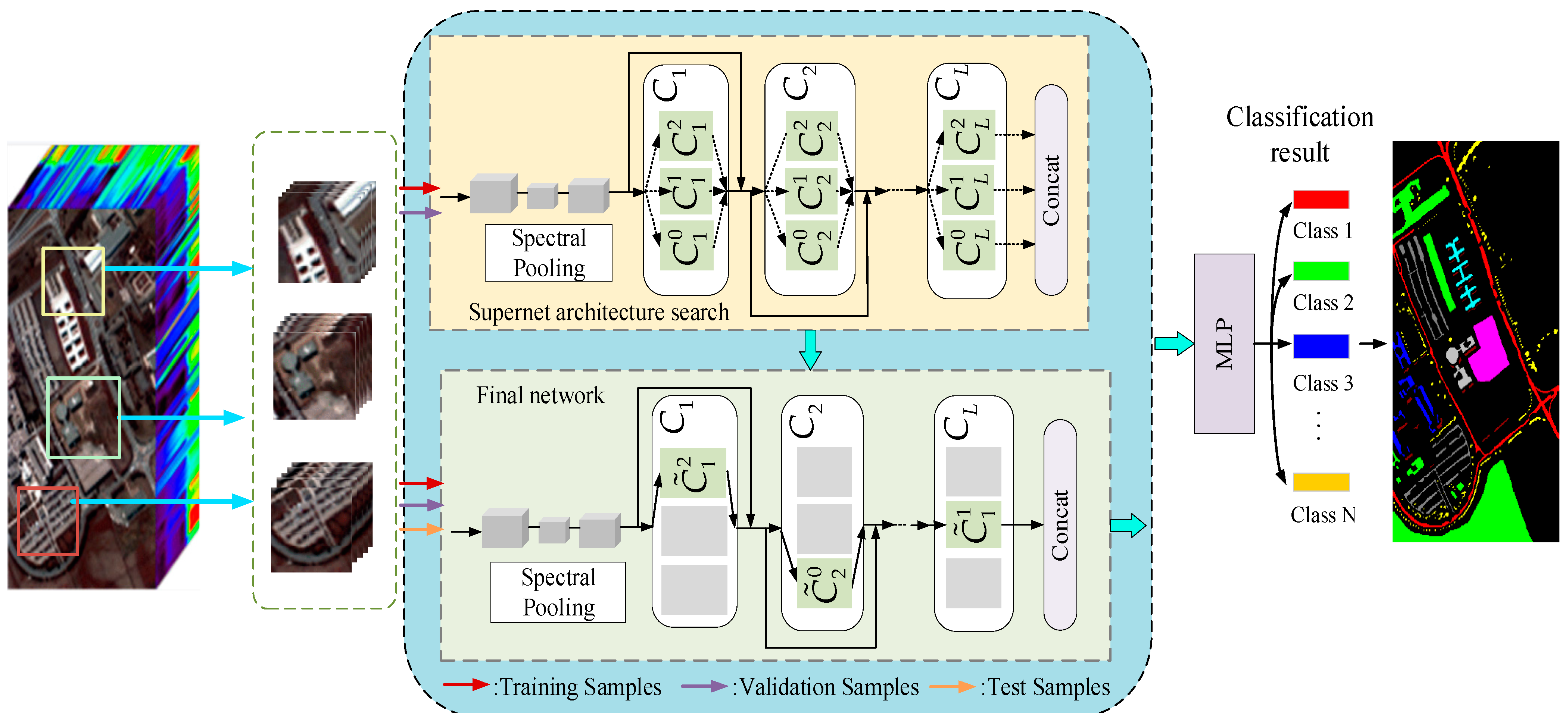
Figure 1. The proposed framework of RFSS-NAS for HSIC.
Remotesensing 16 03123 g001
Figure 2. Receptive field spatial–spectral attention separable convolution operators (K = 3, 5, 7).
Remotesensing 16 03123 g002
Figure 3. The structure of Fused_MBConv.
Remotesensing 16 03123 g003
Figure 4. The Noisy-DARTS search process: (a) building candidate operations between nodes; and (b) the final architecture of topological architecture search.
Remotesensing 16 03123 g004
Figure 5. The classification results of KSC dataset. (a) Ground-truth map. (b) RBF-SVM. (c) CNN. (d) PyResNet. (e) SSRN. (f) 3-D AT-CNN. (g) HNAS. (h) LMSS-NAS. (i) RFSS-NAS.(The red box represents the selected area enlarged for comparison.)
Remotesensing 16 03123 g005aRemotesensing 16 03123 g005b
Figure 6. The classification results of PU dataset. (a) Ground-truth map. (b) RBF-SVM. (c) CNN. (d) PyResNet. (e) SSRN. (f) 3-D AT-CNN. (g) HNAS. (h) LMSS-NAS. (i) RFSS-NAS.
Remotesensing 16 03123 g006
Figure 7. The classification results of HU dataset. (a) Ground-truth map. (b) RBF-SVM. (c) CNN. (d) PyResNet. (e) SSRN. (f) 3-D AT-CNN. (g) HNAS. (h) LMSS-NAS. (i) RFSS-NAS. (The red and blue boxed represent the selected area enlarged for comparison.)
Remotesensing 16 03123 g007aRemotesensing 16 03123 g007b
Figure 8. The searched cell architectures of KSC dataset. (a) Normal cell. (b) Reduce cell.
Remotesensing 16 03123 g008
Figure 9. The searched cell architectures of PU dataset. (a) Normal cell. (b) Reduce cell.
Remotesensing 16 03123 g009
Figure 10. The searched cell architectures of HU dataset. (a) Normal cell. (b) Reduce cell.
Remotesensing 16 03123 g010
Figure 11. The researched normal cell of different architectures: (a) RFSS-NA; (b) RFSS-NAS-Rop; (c) RFSS-NAS-Rtopo; and (d) RFSS-NAS-Rbop.
Remotesensing 16 03123 g011
Figure 12. The researched reduction cell of different architectures: (a) RFSS-NA; (b) RFSS-NAS-Rop; (c) RFSS-NAS-Rtopo; and (d) RFSS-NAS-Rbop.
Remotesensing 16 03123 g012
Figure 13. Visualization of the 2D spectral–spatial features in KSC via t-SNE. (a) Without RFSSA. (b) With RFFSA.
Remotesensing 16 03123 g013
Figure 14. The confusion matrices of KSC, PU, and HU datasets: (a) KSC; (b) PU; and (c) HU.
Remotesensing 16 03123 g014
Figure 15. Learning curves on the KSC dataset. (a) Valid loss vs train loss each epoch. (b) Valid accuracy vs train accuracy each epoch.
Remotesensing 16 03123 g015
Figure 16. Learning curves on the PU dataset. (a) Valid loss vs train loss each epoch. (b) Valid accuracy vs train accuracy each epoch.
Remotesensing 16 03123 g016
Figure 17. Learning curves on the HU dataset. (a) Valid loss vs train loss each epoch. (b) Valid accuracy vs train accuracy each epoch.
Remotesensing 16 03123 g017
Table 1. Information of the search space.
NumberNameOperation
o 1 Skip_connection f ( x ) = x
o 2 Avg_pool_3 × 3Avgpoling (3 × 3)
o 3 Max_pool_3 × 3Maxpooling (3 × 3)
o 4 RFSSA_SepConv_3 × 3RFA-CBMA-Conv2d (3 × 1)-Conv2d (1 × 3)
o 5 RFSSA_SepConv_5 × 5RFA-CBMA-Conv2d (5 × 1)-Conv2d (1 × 5)
o 6 RFSSA_SepConv_7 × 7RFA-CBMA-Conv2d (7 × 1)-Conv2d (1 × 7)
o 7 Fused_MBConv_3_3Conv2d (3 × 3)-SE-Conv (1 × 1)
o 8 Fused_MBConv_3_5Conv2d (3 × 5)-SE-Conv (1 × 1)
o 9 Fused_MBConv_3_7Conv2d (3 × 7)-SE-Conv (1 × 1)
o 10 None f ( x ) = 0
Table 2. The KSC dataset labeled sample information.
No.Class NameColorSampleFalse-Color MapGround-Truth Map
1ScrubRemotesensing 16 03123 i001761Remotesensing 16 03123 i002Remotesensing 16 03123 i003
2WillowRemotesensing 16 03123 i004243
3PalmRemotesensing 16 03123 i005256
4PineRemotesensing 16 03123 i006252
5BroadleafRemotesensing 16 03123 i007161
6HardwoodRemotesensing 16 03123 i008229
7SwapRemotesensing 16 03123 i009105
8GraminoidRemotesensing 16 03123 i010431
9SpartinaRemotesensing 16 03123 i011520
10CattailRemotesensing 16 03123 i012404
11SaltRemotesensing 16 03123 i013419
12MudRemotesensing 16 03123 i014503
13WaterRemotesensing 16 03123 i015927
Total 5211
Sensor: VIRIS; Spectral Bands: 176; Spectral Region: 0.4–2.5 µm; Categories: 13
Table 3. The PU dataset labeled sample information.
No.ClassColorSample NumbersFalse-Color MapGround-Truth Map
1AsphaltRemotesensing 16 03123 i0166631Remotesensing 16 03123 i017Remotesensing 16 03123 i018
2MeadowsRemotesensing 16 03123 i01918,649
3GravelRemotesensing 16 03123 i0202099
4TreesRemotesensing 16 03123 i0213064
5SheetsRemotesensing 16 03123 i0221345
6Bare SoilRemotesensing 16 03123 i0235029
7BitumenRemotesensing 16 03123 i0241330
8Self-Blocking BricksRemotesensing 16 03123 i0253682
9ShadowsRemotesensing 16 03123 i026947
Total 42,776
Sensor: ROSIS; Spectral Bands: 103; Spectral Region: 0.43–0.86 µm; Categories: 9
Table 4. The HU dataset labeled sample information.
No.ClassColorSample NumbersFalse-Color MapGround-Truth Map
1Healthy GrassRemotesensing 16 03123 i0271251Remotesensing 16 03123 i028Remotesensing 16 03123 i029
2Stressed GrassRemotesensing 16 03123 i0301254
3Synthetic GrassRemotesensing 16 03123 i031697
4TreesRemotesensing 16 03123 i0321244
5SoilRemotesensing 16 03123 i0331242
6WaterRemotesensing 16 03123 i034325
7ResidentialRemotesensing 16 03123 i0351268
8CommercialRemotesensing 16 03123 i0361244
9RoadRemotesensing 16 03123 i0371252
10HighwayRemotesensing 16 03123 i0381227
11RailwayRemotesensing 16 03123 i0391235
12Parking Lot1Remotesensing 16 03123 i0401233
13Parking Lot2Remotesensing 16 03123 i041469
14Tennis CourtRemotesensing 16 03123 i042428
15Running TrackRemotesensing 16 03123 i043660
Total 15,029
Sensor: ITRES CASI-1500; Spectral Bands: 144; Spectral Region: 0.36–1.05 µm; Categories: 15
Table 5. Dataset samples’ partition for HSIC.
DatasetCategoriesTraining SamplesValidation SamplesTest SamplesTraining Sample Rate
KSC1330 pixel/category 10 pixel/category46917.4%
PU942,4160.63%
HU1514,4292.99%
Table 6. Classification results of all methods on KSC dataset.
MethodRBF-SVMCNNPyResNetSSRN3-D AT-CNNHNASLMSS-NASRFSS-NAS
Class
192.81 ± 0.7995.94 ± 2.9292.80 ± 9.4898.38 ± 1.1493.57 ± 2.1099.01 ± 0.2599.92 ± 0.18100.00 ± 0.00
286.61 ± 5.1079.58 ± 6.2285.58 ± 8.1794.94 ± 6.3596.83 ± 4.6198.81 ± 0.7799.51 ± 0.7699.51 ± 0.24
373.32±8.3465.81±17.0185.94±7.5096.81 ± 2.3594.12 ± 0.5799.50 ± 0.1299.69 ± 0.64100.00 ± 0.00
454.48 ± 8.6452.27 ± 13.0569.89 ± 10.3185.55 ± 7.0296.50 ± 5.1098.78 ± 0.13100.00 ± 0.00100.00 ± 0.00
560.22 ± 12.1338.73 ± 22.0268.35 ± 14.3077.22 ± 9.1297.46 ± 2.4196.46 ± 0.3197.40 ± 4.2097.90 ± 8.70
665.46 ± 8.3473.97 ± 7.2292.05 ± 12.3292.93 ± 5.1599.04 ± 0.5396.26 ± 0.43100.00 ± 0.00100.00 ± 0.00
776.21 ± 3.8258.28 ± 19.2497.22 ± 2.0794.54 ± 4.5995.31 ± 2.1794.99 ± 0.8299.35 ± 1.93100.00 ± 0.00
886.60 ± 5.0385.67 ± 9.5496.38 ± 2.4697.54 ± 0.9093.19 ± 1.2496.72 ± 0.44100.00 ± 0.00100.00 ± 0.00
988.44 ± 2.6687.21 ± 6.2491.32 ± 12.3798.79 ± 1.2585.37 ± 4.8696.99 ± 0.3599.79 ± 0.3799.72 ± 0.01
1096.30 ± 4.9394.12 ± 1.5199.45 ± 0.9799.65 ± 0.6098.98 ± 1.5095.25 ± 1.02100.00 ± 0.00100.00 ± 0.00
1196.15 ± 1.5298.32 ± 1.4296.34 ± 8.6198.65 ± 1.46100.00 ± 0.0093.35 ± 0.8598.80 ± 1.6798.89 ± 3.67
1293.60 ± 2.6694.37 ± 2.0196.10 ± 2.1997.15 ± 1.2198.08 ± 4.8699.88 ± 0.20100.00 ± 0.00100.00 ± 0.00
1399.67 ± 0.6899.79 ± 0.2499.12 ± 1.2594.55 ± 2.5399.30 ± 1.8499.32 ± 0.38100.00 ± 0.00100.00 ± 0.00
OA (%)87.94 ± 1.5786.31 ± 1.4892.08 ± 1.7296.02 ± 4.8297.97 ± 0.5897.57 ± 0.1398.51 ± 0.2699.83 ± 0.02
AA (%)82.30 ± 2.4978.77 ± 3.0190.13 ± 5.3894.89 ± 3.4786.72 ± 7.4597.72 ± 0.1197.05 ± 1.3599.70 ± 0.03
K × 10086.57 ± 1.7484.77 ± 1.6590.96 ± 1.9796.47 ± 5.3797.69 ± 0.6797.37 ± 0.1498.58 ± 0.3099.78 ± 0.02
Table 7. Classification results of all methods on PU dataset.
MethodRBF-SVMCNNPyResNetSSRN3-D AT-CNNHNASLMSS-NASRFSS-NAS
Class
181.26 ± 5.0884.16 ± 7.7692.35 ± 9.2698.09 ± 1.7792.11 ± 5.2292.63 ± 3.5498.57 ± 0.2697.05 ± 1.89
284.53 ± 3.8190.26 ± 3.9497.02 ± 6.6097.88 ± 0.7798.61 ± 0.7898.92 ± 0.6698.75 ± 0.2499.70 ± 0.12
356.56 ± 16.1738.89 ± 2.2995.08 ± 4.0182.55 ± 12.5092.73 ± 3.5994.14 ± 2.8393.09 ± 1.2399.33 ± 0.17
494.34 ± 3.5092.80 ± 6.2191.13 ± 3.8095.07 ± 6.9595.12 ± 3.5991.68 ± 3.8887.03 ± 7.7098.50 ± 1.74
595.38 ± 3.4094.01 ± 5.9299.83 ± 0.2199.77 ± 0.2292.53 ± 6.5991.65 ± 5.9899.19 ± 0.12100.00 ± 0.00
680.66 ± 7.5476.20 ± 8.7197.68 ± 3.4194.25 ± 1.7198.84 ± 1.0298.99 ± 0.7594.13 ± 1.4999.94 ± 0.07
769.13 ± 11.0446.25 ± 27.8595.05 ± 7.1582.64 ± 14.791.38 ± 4.6390.81 ± 4.6086.78 ± 8.2699.68 ± 0.33
871.16 ± 6.2464.98 ± 3.9683.29 ± 14.2381.60 ± 8.6387.11 ± 3.6591.23 ± 4.1787.93 ± 0.3595.50 ± 3.69
999.94 ± 0.0788.72 ± 9.1598.21 ± 1.4398.89 ± 1.5587.52 ± 6.9286.03 ± 4.1789.10 ± 8.8499.09 ± 1.27
OA (%)82.06 ± 2.7883.35 ± 3.6492.14 ± 10.8794.12 ± 0.7594.82 ± 0.9495.31 ± 0.7096.34 ± 0.2898.79 ± 0.07
AA (%)79.22 ± 5.8775.14 ± 9.1694.40 ± 5.3492.30 ± 1.6592.82 ± 0.9892.86 ± 0.7396.73 ± 1.1098.76 ± 0.15
K × 10075.44 ± 4.2677.63 ± 5.1390.21 ± 12.9792.22 ± 1.0193.41 ± 1.2194.06 ± 0.9096.33 ± 0.4898.65 ± 0.20
Table 8. Classification results of all methods on HU dataset.
MethodRBF-SVMCNNPyResNetSSRN3-D AT-CNNHNASLMSS-NASRFSS-NAS
Class
186.22 ± 5.4794.30 ± 2.2291.48 ± 3.2198.85 ± 0.8490.26 ± 4.7091.02 ± 3.1281.29 ± 1.9799.76 ± 0.06
294.70 ± 0.8391.09 ± 1.8893.41 ± 5.4798.48 ± 1.4088.73 ± 4.3386.90 ± 5.1096.01 ± 3.1091.39 ± 1.35
391.98 ± 7.8999.20 ± 0.3998.63 ± 0.1696.90 ± 0.6786.80 ± 7.2994.29 ± 5.8298.86 ± 4.1597.25 ± 4.32
499.10 ± 0.5598.61 ± 1.1797.35 ± 1.2393.88 ± 7.7690.36 ± 3.2289.40 ± 0.9196.23 ± 2.5699.33 ± 0.45
591.92 ± 2.9493.59 ± 0.3798.40 ± 0.0598.79 ± 0.5597.61 ± 2.3496.50 ± 3.9892.46 ± 2.6396.97 ± 0.06
690.15 ± 0.8598.21 ± 0.0295.65 ± 4.2096.85 ± 0.8686.54 ± 6.0388.19 ± 8.6887.21 ± 9.3897.95 ± 3.97
760.10 ± 6.2092.73 ± 2.4290.37 ± 1.8987.86 ± 6.4880.83 ± 5.0679.33 ± 6.1988.95 ± 5.2698.30 ± 0.75
869.58 ± 6.0597.18 ± 1.1988.49 ± 5.1889.14 ± 11.0690.51 ± 6.2688.66 ± 6.2698.07 ± 0.7498.48 ± 1.94
965.07 ± 7.7794.92 ± 5.4890.72 ± 4.7095.41 ± 2.2885.82 ± 4.1979.77 ± 3.8291.77 ± 4.8897.68 ± 0.79
1059.29 ± 7.6085.33 ± 6.1173.72 ± 8.0391.72 ± 4.9590.53 ± 4.2986.24 ± 6.7895.68 ± 7.3795.39 ± 1.47
1157.10 ± 10.7892.43 ± 6.5492.09 ± 4.3695.55 ± 4.0397.81 ± 2.9697.13 ± 2.4597.07 ± 5.4999.28 ± 0.34
1261.25 ± 6.5293.27 ± 3.1190.44 ± 3.7792.58 ± 1.8389.91 ± 4.2387.71 ± 4.0693.72 ± 8.9195.81 ± 1.55
1360.41 ± 27.3397.36 ± 2.3195.70 ± 2.1796.89 ± 2.6396.85 ± 2.4788.34 ± 10.2188.69 ± 8.9699.49 ± 0.51
1482.35 ± 10.0298.35 ± 0.5098.55 ± 2.3499.03 ± 0.1187.24 ± 4.6492.98 ± 6.6699.21 ± 3.1591.49 ± 5.42
1599.48 ± 0.0699.25 ± 0.8699.20 ± 1.0898.05 ± 0.8990.91 ± 6.8092.74 ± 5.1697.05 ± 1.4094.20 ± 2.90
OA (%)76.15 ± 2.7493.55 ± 1.6491.29 ± 1.6594.69 ± 1.9389.59 ± 0.9188.40 ± 1.6293.07 ± 0.4196.91 ± 0.20
AA (%)78.97 ± 0.6294.57 ± 1.4393.11 ± 0.0895.87 ± 1.3590.04 ± 0.7089.28 ± 1.7893.48 ± 0.5796.86 ± 0.05
K × 10074.17 ± 2.9894.10 ± 1.7790.59 ± 1.7994.26 ± 2.0988.76 ± 0.9887.42 ± 1.6592.50 ± 0.4896.65 ± 0.22
Table 9. Structural effectiveness analysis of RFSS-NAS.
ModelsRFSS-NASRFSS-NAS-RopRFSS-NAS-RtopoRFSS-NAS-Rbop
OA (%)99.8599.3899.0899.50
AA (%)99.9098.9898.6399.51
K × 10099.8399.1798.7899.45
Table 10. Ablation experiments of each component (Pavia University dataset).
Fused_MBConvRFSSANoisy-DARTS OA (%)AA (%)K × 100
97.69 ± 1.3097.15 ± 2.1197.30 ± 2.18
96.36 ± 1.5396.68 ± 0.7296.06 ± 0.57
98.20 ± 0.2998.29 ± 0.8398.37 ± 1.13
98.79 ± 0.0798.76 ± 0.1598.65 ± 0.20
Table 11. Ablation experiments on loss functions.
DatasetLossOA (%)AA (%)K × 100Test Time (s)Params (M)
KSCSM Loss98.55 ± 0.4298.57 ± 0.4198.27 ± 0.2310.011.39
PL Loss99.01 ± 0.2298.62 ± 0.5798.94 ± 0.6110.301.42
SM Loss + PL Loss99.83 ± 0.0299.70 ± 0.0399.78 ± 0.0210.371.46
PUSM Loss98.32 ± 0.1297.98 ± 0.4498.03 ± 0.1710.851.49
PL Loss98.25 ± 0.0397.50 ± 0.1897.88 ± 0.2211.211.54
SM Loss + PL Loss98.79 ± 0.0798.76 ± 0.1598.65 ± 0.2012.991.61
HUSM Loss95.41 ± 0.1695.95 ± 0.0795.19 ± 0.127.281.25
PL Loss96.21 ± 0.1195.97 ± 0.1396.10 ± 0.068.561.31
SM Loss + PL Loss96.91 ± 0.2096.86 ± 0.0596.65 ± 0.229.821.37
Table 12. Comparison of parameter quantity and running time of different methods on three datasets.
MethodsKSCPUHU
Params (M)Train (m)Test (s)Params (M)Train (m)Test (s)Params (M)Train (m)Test (s)
3D-CNN0.146.185.570.099.946.210.158.795.93
PyResNet85.1022.387.1684.21175.4152.6784.7365.8821.62
SSRN1.258.212.470.8363.1016.191.0647.7715.93
3-D AT-CNN0.1219.417.720.1911.225.790.0913.026.11
HNAS2.7031.638.942.7315.358.892.6430.819.42
LMSS-NAS0.089.398.230.1610.599.290.057.829.01
RFSS-NAS1.4612.1410.371.6112.9212.991.3710.889.82
Table 13. The classification performance of the algorithm on different types of noise.
DatasetNoise TypeOA (%)AA (%)K × 100
KSCw/o Noise99.57 ± 0.2699.01 ± 0.1299.52 ± 0.11
Gaussian99.63 ± 0.1499.66 ± 0.0799.59 ± 0.17
Uniform99.83 ± 0.0299.70 ± 0.0399.78 ± 0.02
Table 14. Classification performance with different proportions of training samples using PU dataset.
Training Sample SizesOA (%)AA (%)K × 100
0.10%66.82 ± 0.2770.63 ± 0.3459.90 ± 0.26
0.21%79.06 ± 0.3277.34 ± 0.2673.62 ± 0.31
0.31%82.74 ± 0.1286.15 ± 0.2778.27 ± 0.14
0.42%90.40 ± 0.0990.34 ± 0.1187.66 ± 0.06
0.53%94.70 ± 0.1393.81 ± 0.0793.04 ± 0.11
0.63%98.79 ± 0.0798.76 ± 0.1598.65 ± 0.20
Disclaimer/Publisher’s Note: The statements, opinions and data contained in all publications are solely those of the individual author(s) and contributor(s) and not of MDPI and/or the editor(s). MDPI and/or the editor(s) disclaim responsibility for any injury to people or property resulting from any ideas, methods, instructions or products referred to in the content.