Article

Refined Intelligent Landslide Identification Based on Multi-Source Information Fusion

1
School of Architecture and Civil Engineering, Chengdu University, Chengdu 610106, China
2
Key Laboratory of Earth Exploration and Information Techniques, Ministry of Education, Chengdu University of Technology, Chengdu 610059, China
3
The State Key Laboratory of Information Engineering in Surveying, Mapping and Remote Sensing, Wuhan University, Wuhan 430079, China
4
College of Earth Sciences, Chengdu University of Technology, Chengdu 610059, China
5
China Building Materials Southwest Survey and Design Co., Ltd., Chengdu 610052, China
6
State Key Laboratory of Geohazard Prevention and Geoenvironment Protection, Chengdu University of Technology, Chengdu 610059, China
7
Sichuan Earthquake Agency, Chengdu 610041, China
*
Author to whom correspondence should be addressed.
Remote Sens. 2024, 16(17), 3119; https://doi.org/10.3390/rs16173119
Submission received: 19 June 2024 / Revised: 17 August 2024 / Accepted: 22 August 2024 / Published: 23 August 2024
(This article belongs to the Special Issue Application of Remote Sensing Approaches in Geohazard Risk)

Abstract

:
Landslides are most severe in the mountainous regions of southwestern China. While landslide identification provides a foundation for disaster prevention operations, methods for utilizing multi-source data and deep learning techniques to improve the efficiency and accuracy of landslide identification in complex environments are still a focus of research and a difficult issue in landslide research. In this study, we address the above problems and construct a landslide identification model based on the shifted window (Swin) transformer. We chose Ya’an, which has a complex terrain and experiences frequent landslides, as the study area. Our model, which fuses features from different remote sensing data sources and introduces a loss function that better learns the boundary information of the target, is compared with the pyramid scene parsing network (PSPNet), the unified perception parsing network (UPerNet), and DeepLab_V3+ models in order to explore the learning potential of the model and test the models’ resilience in an open-source landslide database. The results show that in the Ya’an landslide database, compared with the above benchmark networks (UPerNet, PSPNet, and DeepLab_v3+), the Swin Transformer-based optimization model improves overall accuracies by 1.7%, 2.1%, and 1.5%, respectively; the F1_score is improved by 14.5%, 16.2%, and 12.4%; and the intersection over union (IoU) is improved by 16.9%, 18.5%, and 14.6%, respectively. The performance of the optimized model is excellent.

1. Introduction

Landslides are among the most impactful types of geological disasters worldwide, posing serious threats to the lives and property of people everywhere due to their suddenness and uncertainty. In particular, China is significantly affected by geological disasters [1]. According to the China Statistical Yearbook (https://www.stats.gov.cn/sj/ndsj/2023/indexch.htm, accessed on 11 May 2024) released by the National Bureau of Statistics (NBS), a total of 5659 geological disasters occurred in 2022, of which 3919 were landslides, accounting for 69.2% of these disasters [2]. In this paper, the term “landslide” refers specifically to landslides, where rock and soil bodies slide along a certain sliding surface as an entire piece of mass under the influence of natural or anthropogenic factors. The economic losses caused by the landslides that occurred in 2022 amounted to CNY 1502.81 million. In order to reduce the hazards posed by landslide disasters, governmental disaster reduction departments have organized landslide censuses and detailed investigations at different scales and with different accuracies, and they have identified numerous potential landslide disaster sites, thereby providing an important foundation for landslide disaster reduction efforts [3]. To date, landslide surveys and detailed investigations have mainly been conducted utilizing remote sensing interpretation and field trips. The identification of landslides through fieldwork is not only time-consuming and laborious, but it is also limited by the vegetation on the surface of the slope and the professional ability of the inspectors [4].
Remote sensing, with its outstanding advantages of large-scale synchronous observation and cost-effectiveness, is being increasingly used for the investigation of geological disasters. Although the identification of landslides using remote sensing interpretation methods has greatly improved in terms of efficiency, existing remote sensing-based landslide interpretation methods are primarily visual interpretation methods (i.e., involving the interpretation of visual aerial and satellite remote sensing imagery and manual visual interpretation with the help of some auxiliary equipment); however, these methods not only have a low interpretation efficiency but also a high rate of omission. This is also one of the reasons why many landslide hazards still exist, even though many landslide censuses and detailed investigations have been conducted [5]. In this context, the use of rapidly developing image-processing technology in the construction of an automatic landslide identification model based on remote sensing imagery in order to improve the efficiency and accuracy of landslide identification can be considered a more effective method for landslide identification, providing a basis for landslide disaster mitigation [6]. Landslide identification based on remote sensing images has a long history, where most sample objects selected for landslide identification in previous studies were seismic-type landslides; in this context, the vegetation overlying the landslide mass is destroyed, and the spectral characteristics of the ground surface significantly differ from those of normal ground surfaces. These landslides are relatively easier to recognize, and computer recognition technology for this type of landslide based on remote sensing imagery is relatively mature [7]. However, the spectral characteristics of most landslides are not significant in that the spectral characteristics and topographic features should be integrated to identify landslides at different stages of development. Landslides change the original surface structure and destroy the original topography, drainage, and vegetation conditions. These features are very prominent in remote sensing images, providing automatic identification possibilities of landslides based on remote sensing. Mapping the process of the visual interpretation of landslides by professionals to the computational space is key to solving the automatic landslide identification problem; in particular, it is necessary to incorporate other feature factors besides landslide images in the process of landslide identification.
In recent years, deep learning technology has realized remarkable achievements in remote sensing image-processing applications [8]. Deep learning, as a derivative field of artificial intelligence, involves the use of deeper neural networks. A core goal of such approaches is to present image data as multi-level associative structures, which can be represented as multi-scale semantic feature associations, gradually linking local features to global features and thus realizing a high-level feature representation of low-level features. In semantic segmentation, high-level feature expressions can represent semantic information that guides the segmentation process [9]. Deep learning does not require the artificial extraction of features because—through the model’s own learning ability—the essential features and intrinsic laws in image data can be gradually extracted, providing good adaptability. After iteratively adjusting the model parameters, the model is able to better learn and construct high-level feature structures of the image from the training image samples in order to obtain optimal segmentation performance results. As a result, a semantic segmentation model that can be automated and adapted to a given task is obtained. In the field of semantic segmentation, many techniques have been found to further enhance the expression of advanced semantic information, thus improving the segmentation accuracy of models [10,11,12]. The transformer approach has achieved remarkable results in the translation task. Connecting the encoder and decoder through an attention mechanism, it is able to efficiently direct attention to the important positions in the input sequence, thus achieving better performance than some CNN networks. The first transformer to be applied to computer vision tasks was the vision transformer (ViT), and numerous experiments have shown that this constitutive converter structure achieves feature extraction results comparable to those of CNNs [13,14]. ViT uses the same image facet size at each stage in the process of extracting image features. This processing method ignores feature information at different scales in high-resolution remote sensing images. The Swin Transformer algorithm was optimized on the basis of ViT, incorporating a new pyramid-stage processing method and a sliding window to realize efficient transformer computation.
For this study, we chose Ya’an City, Sichuan Province, as the study area and constructed a landslide sample dataset for the study area from 2021 to 2023. As landslide hazards account for a relatively small proportion of the study area, in order to address the problem of low recognition accuracy for a few target classes, we effectively improved the landslide hazard recognition accuracy by fusing the features of multi-source data and introducing the boundary loss function.
The main contributions of this study are as follows:
(1)
We constructed a sample library for landslide recognition in Ya’an City with multi-source features.
(2)
We analyzed the learning process of the deep learning model on multi-source feature samples using a heat map.
(3)
We constructed a Swin Transformer-based model based on landslide recognition and introduced a boundary loss function to address the problem of low recognition accuracy for a few target classes. We compared our model with classical networks, and it was observed that, after multi-source feature fusion, the model effectively solved the abovementioned problems and improved landslide recognition accuracies.
(4)
We explored a potential application of the Swin Transformer-based model in landslide detection. Based on the Bijie landslide dataset, the expressiveness of the Swin Transformer-based model based on the boundary constraint function and multi-source feature fusion was explored in order to validate its effectiveness and explore its generalization ability.

2. Materials

2.1. Study Area

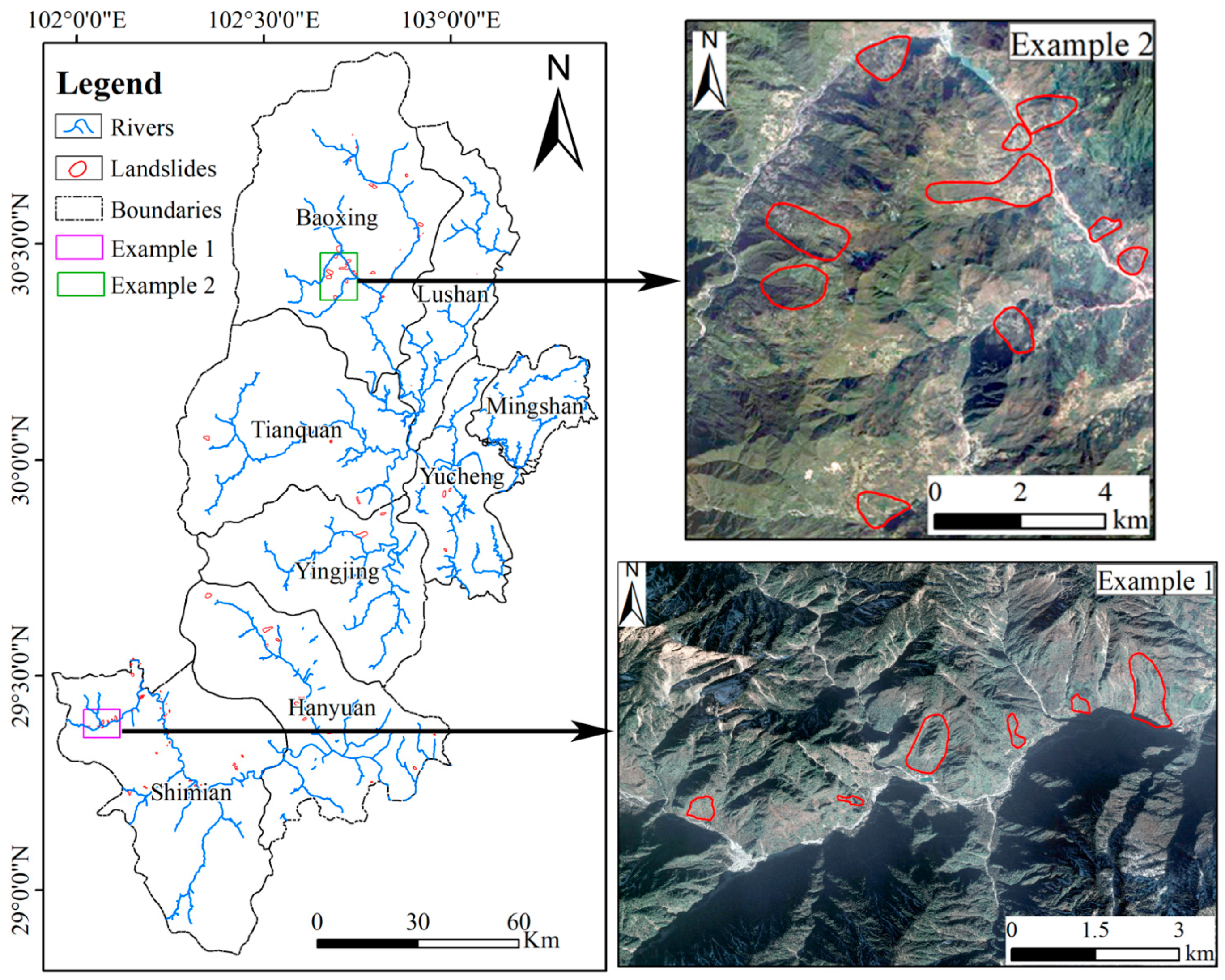
Ya’an City is located in the western part of Sichuan Province (1019°56′–102°28′E, 28°51′–30°56′N). As Ya’an is located in an area characterized by mountainous terrain, the terrain is complicated by a great variation in altitude, resulting in an evident gradual decrease in temperature with increasing altitude. It has a high annual precipitation and heavy rainfall in the summer; hence, it is named “Rainy City.” The crust of this region is in active motion, and the fracture zones are widely distributed. These active fracture zones not only affect the stability of the regional crust but may also trigger geological disasters, such as landslides. The city has jurisdiction over Yucheng, Meishan, Xingjing, Hanyuan, Shimian, Tianquan, Lushan, and Songxing, which include two districts and six counties (Figure 1) [15].

2.2. Landslide Identification Database

2.2.1. Visual Interpretation of Landslides

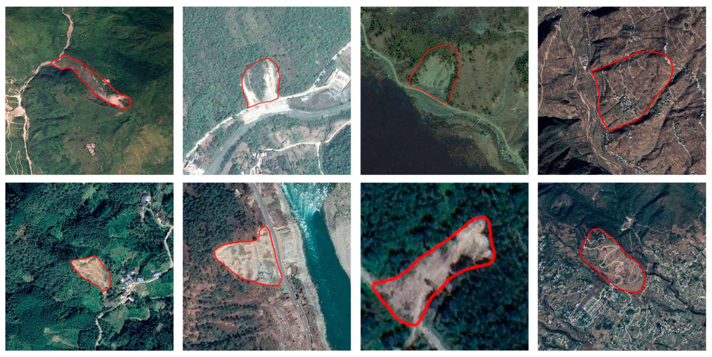
For this study, a detailed landslide hazard interpretation was completed in Ya’an based on field landslide site survey data for 2021–2023 from the Ya’an Bureau of Natural Resources and Planning, as well as high-resolution Google Earth imagery. The steps were as follows: 1. We overlaid the known landslide sites with Google Earth images of Ya’an, and the location and extent of the landslides were initially determined; 2. Staff experienced in landslide interpretation carefully outlined the landslide boundaries according to the texture and color characteristics of each landslide on the images, and some landslides that could not be identified in the images were removed. The detailed landslide interpretation results are shown in Figure 2.
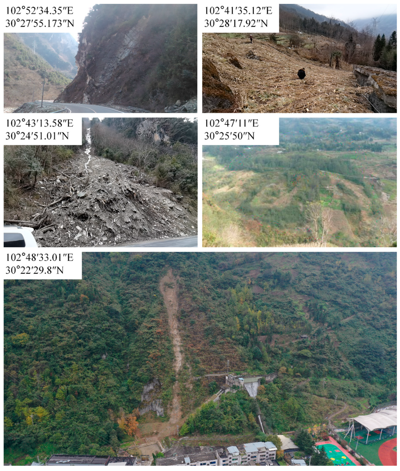
Some of the landslide field verification images are shown in Figure 3.

2.2.2. Database Production for Multi-Source Data

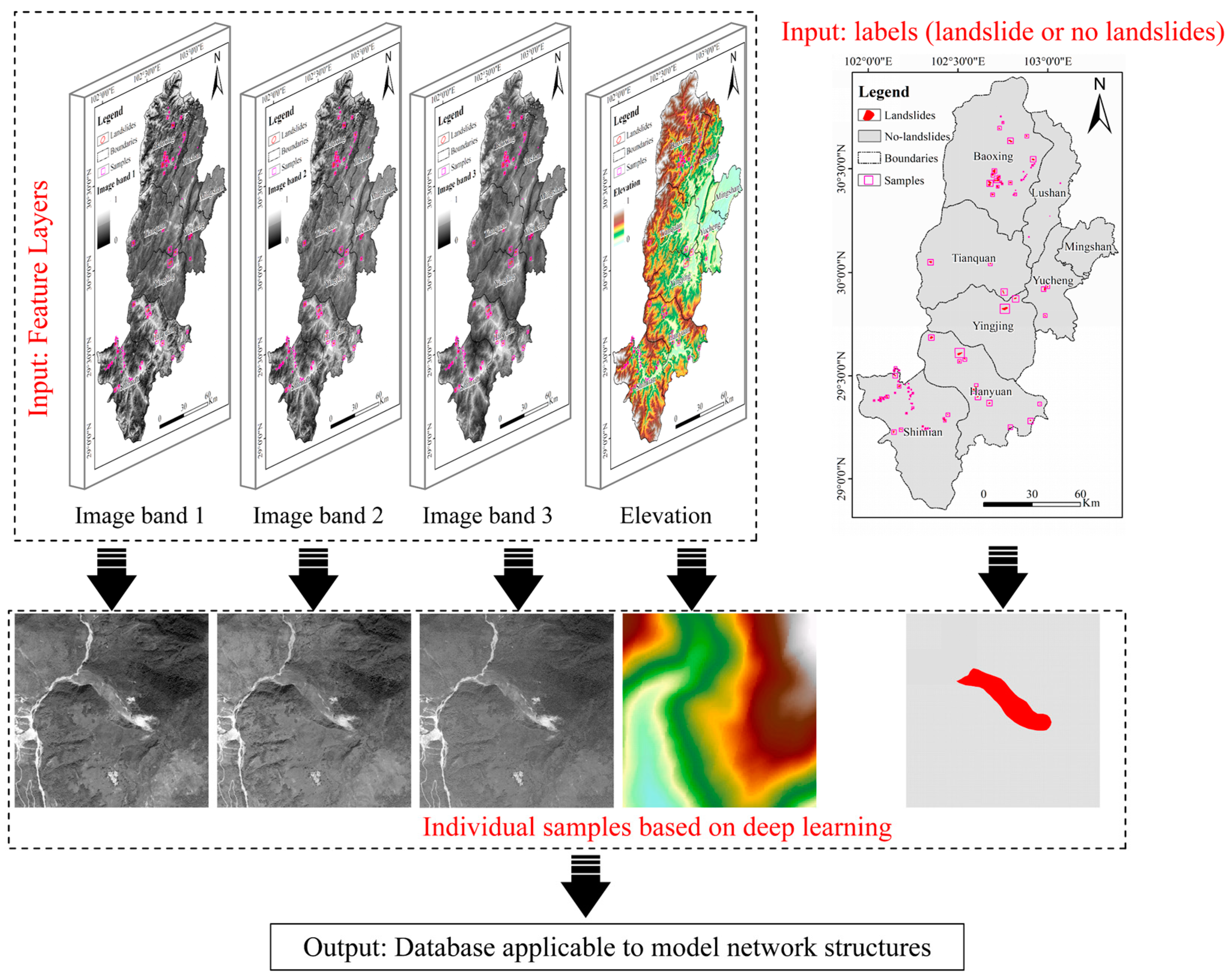
Optical satellite imagery and a digital elevation model (DEM) were used to compile a multi-source database for landslide identification. The historical optical satellite images were provided by Google Earth. The images displayed on Google Earth integrate various data such as aerial photos, satellite images, remote sensing, and a geographic information system (GIS), which are spliced together according to the geographic coordinates and certain mathematical rules, resulting in rich imagery, comprehensive information, and a balance between data accuracy and display realism. The optical images used in this study were captured in 2023, and they have excellent image quality, no cloud cover, and a ground resolution of 2.15 m. In the model training and recognition phase, DEM data were added as the first dimension of the data input, in addition to the red, green, and blue (RGB) satellite image information used to provide auxiliary data for establishing a high-precision landslide intelligent recognition model and to further improve the recognition accuracy of the network. DEM data were obtained from the 1:10,000 DEM of Ya’an City with an accuracy of 5 m, and the range was consistent with that of the images. All data were mapped to the WGS_1984_UTM_Zone_48N coordinate system.
As the size and extent of each landslide in the images differed, the edges of each landslide were extended in all directions when the landslide samples were cropped, and a variety of backgrounds were added to the landslide samples using the outward cropping operation, which helped the network model to learn the unique features of the landslides themselves without interference from the backgrounds. In this study, a total of 108 landslide hazards were identified, and 306 positive samples of landslide instances were produced by combining historical images. Examples of landslide instances are shown in Figure 4.
Sample points identified as non-landslide features were manually selected as negative samples on the satellite images, including non-landslide samples such as mountains, villages, roads, rivers, forests, and farmland. A total of 306 non-landslide samples were used in this study.
Applying a deep learning model for landslide hazard identification requires the creation of a dataset that is suitable with respect to the network structure, potentially requiring the dimensionality of the dataset to be increased in geospatial terms, where each sample is a multi-dimensional matrix containing the information of neighboring pixels. Considering the influence of neighboring pixels on the target elements, the spatial information of landslides is extracted by expanding a single pixel into a two-dimensional pixel matrix consisting of the location and points surrounding it. In order to improve the performance of the network and reduce the risk of overfitting, it was necessary to set the features and labels according to the sample’s information during the construction of the dataset. The dimensions of the pixel matrix, as well as the number of landslide influence factors, together constitute the features of the samples. Whether or not a landslide had occurred at the location corresponding to the pixel matrix was used as a condition to label the samples, with 1 indicating that a landslide had occurred and 0 indicating that a landslide had not occurred. The pixel values of all input feature layers also needed to be normalized within the range of 0–1. The database production process is depicted in Figure 5.

3. Methods

3.1. Swin Transformer

The vision transformer (ViT), as a model representative of the application of transformers in image processing, has achieved better results than traditional CNNs in the field of image recognition, which proves that the transformer is able to replace CNNs in image processing to a certain extent; thus, it has excellent application prospects [16,17]. The shifted window (Swin) transformer modifies the original multi-head self-attention (MSA) structure of the transformer and introduces a window-based MSA (W-MSA) structure, which decomposes the image into multiple non-overlapping windows and calculates the attention in each window separately [18,19], significantly reducing the computation load compared to calculating the attention of the entire picture, as is carried out in ViT. In addition, in order to address the problem of features not being transferred between different windows, the Swin transformer also includes a shifted window-based MSA (SW-MSA) structure, which enhances the recognition accuracy of the network by transferring feature information from different windows through shifting their positions [20]. The Swin transformer model structure and some hyperparameters are shown in Figure 6.
Similarly to the ViT, after entering the Swin transformer, the images are first processed using the patch partition structure for chunking and flattening in the channel dimension. After this, these feature maps pass through four stages to extract the feature information [21]. In the first stage, each block is linearly transformed and then fed into two consecutive Swin transformer blocks [22]. In the subsequent stages, in order to further extract the features and reduce the size of the feature map, the feature map is down-sampled utilizing patch merging, and it is then inputted into the next Swin transformer block [23]. The patch-merging structure divides each neighboring pixel of 2 × 2 size into a patch, and the pixels at the same position in each patch are then divided into two patch-merging blocks and spliced in the depth direction. Next, the feature map is fed into the layer normalization (LayerNorm) layer for normalization; finally, it is downscaled in the depth direction using a fully connected layer. After down-sampling utilizing a patch-merging structure, the width and height of the feature map are reduced to half of the previous values, and the depth is doubled compared to its previous value [24].
The Swin transformer block is the core component of the Swin transformer, and it is composed of two consecutive transformer modules in series, forming the basis upon which the Swin transformer achieves efficient feature extraction and classification [25]. Compared with the traditional transformer module, it replaces the MSA part with W-MSA and SW-MSA structures [26]. Assuming that the size of the input feature map is H × W and the window size of the Swin transformer is set to M × M, when the feature map enters the Swin transformer block, it is segmented by W-MSA into HM × WM windows with a size of M × M; following this, self-attention computation is carried out for each window. Next, the feature map is passed through the multi-layer perceptron (MLP) module, and residual connections are introduced [27]. This structure significantly reduces the computational effort compared to the traditional transformer module; however, as self-attention computation is only performed within the windows, no information can be transferred from window to window [28]. Therefore, the feature maps are obtained after the W-MSA structure passes through the SW-MSA structure again, which shifts the position of the window by M/2 pixels in both the horizontal and vertical directions to complete the transfer of feature information between the different windows [29]. In order to improve robustness and generalization abilities through training, a LayerNorm layer is included between each structure for normalization; finally, the feature extraction results are output through the MLP module.

3.2. Loss Functions

3.2.1. Binary Cross-Entropy (BCE)

The loss function measures the predicted values against the true values: the smaller the model loss, the better the generalization performance of the model [30]. The ultimate goal of model training is to achieve minimization of the loss function under conditional constraints [31]. When considering different tasks, the selected loss function also differs [32]. As its mathematical form is simpler to calculate, the cross-entropy loss is often used as the loss function for training models [33]. The binary cross-entropy (BCE) loss function is based on the cross-entropy loss function but adds proportional weights (0.5) to the number of positive and negative samples. The cross-entropy loss function is used in binary classification problems and is particularly suitable when there is a probabilistic output and only two types of labels (usually labeled 0 and 1) [34]. In machine learning and deep learning, when we train a model to predict the probability of an event occurring, the BCE loss helps to measure the gap between the probability distribution predicted by the model and the actual observed labels, providing a basis for optimizing the model [35]. The BCE loss function can be expressed as follows [36]:
L B C E = 1 N i = 1 N [ y i log ( p i ) + ( 1 y i ) log ( 1 p i ) ]
where N is the number of image pixels, and yi∈{0, 1} [33] is the label category of pixel i in the image, where yi = 1 denotes landslide slopes and yi = 0 denotes non-landslide slopes. The probability of predicting a pixel i as having label yi is denoted as pi∈[0, 1].

3.2.2. Boundary Loss Function

There is usually a severe category imbalance problem in landslide image recognition; that is, the size of the target foreground region (the extent of the landslide) is often several orders of magnitude smaller than that of the background region (other features). This is due to the fact that landslides are relatively rare in nature, compared to other landforms.
The cross-entropy loss function, which is commonly used in the field of landslide identification, has a well-known drawback in highly unbalanced cases; namely, it assumes that all of the samples and categories are of equal importance, which usually leads to training instability and causes the decision boundaries to be biased towards a high number of categories [37]. A common strategy for the category imbalance problem is to down-sample a high number of categories to re-balance the prior distribution of the categories; however, this strategy limits the use of training images. Another strategy is weighting: assigning greater weights to categories with a small number of samples and smaller weights to categories with a large number of samples. Although this method is effective for some imbalance problems, difficulties are still faced when dealing with extremely imbalanced data. The cross-entropy gradient computed over a few pixels usually contains noise, and assigning larger weights to a few categories further increases this noise, thus leading to unstable training [38]. Considering these problems associated with the BCE loss, researchers have proposed a boundary-based loss function, which takes the form of a distance metric on the contour space rather than the region space. Instead of integrating over regions, the boundary loss computes integrals over the boundaries between regions, thus alleviating the problems associated with region loss in highly unbalanced segmentation problems [39].
In order to construct the boundary loss, we first calculate the closest distance from the landslide area of the real label (foreground) to the background d F i (Euclidean distance between the pixel points). We also calculate the closest distance from the background of the real label to the landslide area (foreground) d B j . The expression is as follows [40]:
d F i = min j B ( ( x i x j ) 2 + ( y i y j ) 2 ) , ( i F )
d B j = min j F ( ( x j x i ) 2 + ( y j y i ) 2 ) , ( i B )
where F denotes the set of foreground pixel points, B is the set of background pixel points, and x and y are the horizontal and vertical coordinates where the pixel points are located, respectively. The weight function for the boundary penalty is then obtained by combining d F i and d F i :
W b o u n d a r y k = 1 d F k , ( k F ) d B k , ( k B )
When the pixel belongs to the background and is far away from the boundary, it will be assigned a larger penalty weight. When the pixel belongs to the foreground and is the boundary, its penalty weight is 0. When the pixel belongs to the foreground and is not the boundary, its weight is negative. Finally, the boundary penalty loss function is defined as follows [41]:
L b o u n d a r y = 1 N k N p k W b o u n d a r y k
where pk is the prediction probability of pixel k and N is the number of pixel points in the entire image. In the process of gradient descent, if a pixel point is predicted to be outside the range of the landslide region, a positive gradient will be obtained, and, therefore, the prediction probability will be reduced. In contrast, a negative gradient inside the landslide region will increase the prediction probability during gradient descent.

3.3. Precision Evaluation Indicator

In landslide identification experiments, selecting appropriate evaluation indices is crucial to better reflect the model’s real performance. For all of the experiments conducted in this study, precision (P), recall (R), F1-score (F1), intersection over union (IoU), and overall accuracy (OA) were used as evaluation indices to measure the performance of the model [42]. For the evaluation metrics, the higher the P, the more accurate the detected pixels, and a higher recall rate indicates that fewer wrong pixels were identified by the model. The F1 score takes into account both the precision and recall rate of the classification model, providing a balanced evaluation of the model’s performance. IoU is used to measure the correlation between the real and the predicted values, and the OA reflects the overall precision of the prediction results, which was used as an evaluation index to measure the model performance [43,44]. Both indices range from 0 to 1, with higher values indicating better prediction results. The index formulas are as follows:
P = T P T P + F P
R = T P T P + F N
F 1 = 2 × P × R P + R
I o U = T P T P + F P + F N
O A = T P + T N T P + F P + T N + F N
where TP (true positive) denotes the true-positive class, FP (false positive) is the false-positive class, FN (false negative) is the false-negative class, and TN (true negative) is the true-negative class.

3.4. Experimental Environment Settings

The proposed semantic segmentation model was implemented using the Pytorch deep learning framework, leveraging its end-to-end machine learning capabilities and using Python as the development language. Its ability to carry out inverse auto-derivation provides a great advantage in the computational process of deep learning tasks. Essential functionalities for building a neural network architecture, such as basic convolution, activation, and pooling, are provided by the torch.nn library. In addition, a graphics processing unit (GPU) was introduced to improve the efficiency of the code. The utilized experimental environment and configuration are described in Table 1.

4. Experimental Analysis

4.1. Training Details

4.1.1. Model Training Strategies

The Swin transformer-based model was implemented using the open-source deep learning library Pytorch, and for our experiment, the crop size was set to 256. First, the input source images were randomly cropped to ensure a consistent resolution of 256 × 256 for all images processed using the model. The initial loss function was set as the cross-entropy loss, and the initial learning rate was set as 0.00013. The SGD+Momentum stochastic optimization algorithm was used to train the model; the momentum of the optimization algorithm was 0.9, and the weight decay factor was 0.0005. Each training round consisted of 100 rounds, and the batch size (batch size) was 4. After the completion of each round of training, the validation dataset was used to evaluate the performance of the model at that stage, and the optimal model was then preserved for comparison purposes. Finally, a model with the best segmentation effect was obtained.
Due to the deeper layers of the network model proposed in this study and the up-sampling process, the entire training process is highly time-consuming. Therefore, in the training of deep learning models, researchers generally use the pre-training method, which involves initializing the parameters of the training model using model parameters with better convergence. In this study, we used the method illustrated in Figure 6 to carry out the model-training process. First, we used the proposed backbone network to carry out training on an easy-to-classify dataset (ImageNet) and saved the trained parameters; then, we carried out training again on the collected landslide dataset. The model was initialized to use the pre-training parameters of the backbone network, and the constant updating of the loss value and the weights helped the model adapt to the landslide dataset, reducing the time required for model training while greatly improving classification accuracy during feature extraction. The pre-training process of the model is depicted in Figure 7.

4.1.2. Online Data Enhancement

The learning ability of a neural network mainly depends on the number of data samples, which affects the generalization ability and robustness of the model. When the amount of data is limited, the network is prone to overfitting the data. Furthermore, labeling additional data is both time-consuming and labor-intensive [45]. To address these issues, when faced with limited image data, enhancing the dataset to expand the sample size is necessary. Data enhancement can be divided into offline data enhancement and online data enhancement. Offline data enhancement refers to the preprocessing of data before data training, and it is commonly performed using methods such as scaling and cropping. In contrast, online data enhancement refers to the enhancement of data before each iteration in the training process in order to enlarge the scale of the dataset and improve the generalization ability and stability of the model [46]. The main steps of online enhancement are as follows [47]: (1) the model starts training; (2) a small batch of data is extracted from the original dataset according to specific or random rules; (3) the small batch of original data is sent to the data intensifier, which then carries out geometric, color, and pixel transformations according to specific rules; (4) the data enhancer inputs the enhanced small batch of data into the model for training; and (5) steps (2) to (4) are repeated until the training is completed. Figure 8 presents a schematic diagram of the workflow of the online data enhancement method.
In this study, data enhancement was carried out by means of a two-dimensional online data enhancement module—including geometric shape and image color transformations—in order to improve the training effect of the model. Particular attention should be paid to the fact that as the elevation data are formatted as a single-band image, the color change has no meaning; thus, only geometric transformation is performed on these data.

Geometric Shape Transformation

The geometric transformation of image data generally includes flipping, rotating, cropping, deforming, scaling, and other operations [48]. After a large number of experiments, for image recognition or classification, the flipping and rotating transformations of the image were found to effectively enhance the data. Flipping is a method similar to mirror folding; in contrast, rotating refers to clockwise or counterclockwise rotation. It should be noted that it is best to carry out rotations by an interval of 90° to 180°; otherwise, there will be inconsistency in the image sample’s scale. In addition, the enhanced images obtained via flipping and rotating differ from the original image only in terms of the direction and angle, while the image size remains the same [49,50]. In this study, we chose to use random rotation and flipping methods to carry out the data enhancement of landslide sample images. When geometric transformations were performed on the training images, the labels were also transformed accordingly; otherwise, the labels would not correspond to the transformed images. Examples of the geometrically transformed images are shown in Figure 9.

Image Color Transformation

The color transformation process does not directly change the information in the image sample itself: it only selects a portion of the original image according to certain rules or re-distributes the pixels of the original image according to a certain ratio.
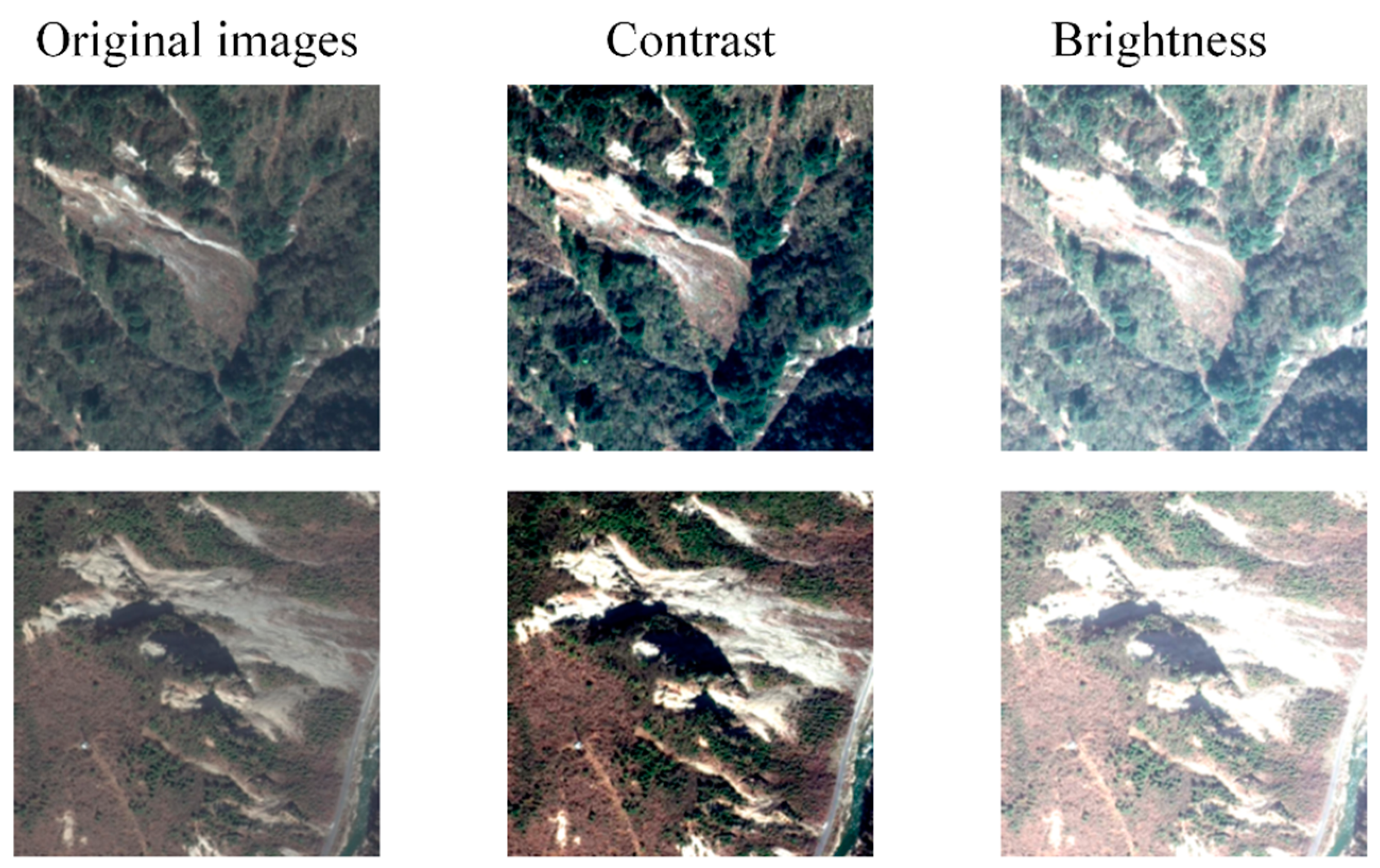
In simple terms, the different colors in an image represent different pixels. Therefore, color transformation is conducted to enhance an image by changing the information (pixels) in the image itself. The general methods of color transformation include contrast, brightness, color enhancement, and image-sharpening transformations [51]. Among them, brightness transformations involve adjusting the brightness and darkness of the original image, contrast transformations involve transformation by adjusting the brightness ratio between the brightest and darkest parts of the image, and image sharpening involves making the image clearer by compensating for the color at the edges of the image. An example of partial color transformation of a landslide image is shown in Figure 10.

4.2. Analysis of Experimental Results

4.2.1. Comparison of Different Feature Extraction Networks

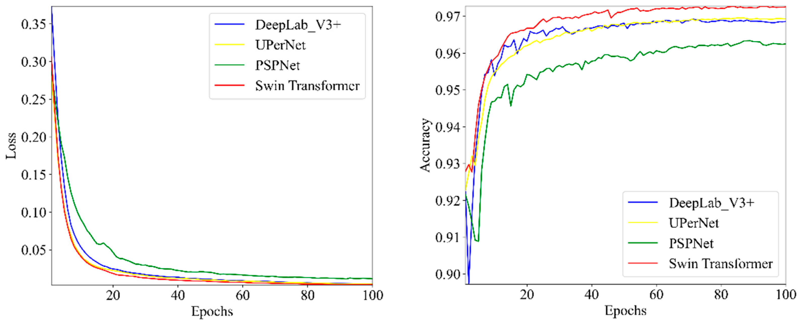
For this experiment, the landslide dataset was divided into training, validation, and testing sets. The model performances of the Swin transformer-based network and classical feature extraction networks—UPerNet, pyramid scene parsing network (PSPNet), and DeepLab_v3+—were compared. Figure 10 presents graphs showing loss and accuracy changes during the training process for the above models. As observed in Figure 11, UPerNet, Swin transformer, and DeepLab_v3+ fit faster during the training process, and the Swin transformer-based model exhibited the highest training accuracy. Meanwhile, PSPNet had a slower fit and the lowest training accuracy. The results indicate that the Swin transformer-based model reached the convergence state earlier, exhibited more stable and effective training performances, did not overfit, and had a stronger generalization ability compared to the other models.
Table 2 presents the results of the comparison between the different models in the landslide testing set.
When evaluating the prediction performance of different models, several indicators need to be considered to make a judgment. From the above results, it can be observed that the Swin transformer-based model outperformed the other models in terms of the OA, F1-score, IoU, and R metrics. The OA of the Swin transformer-based model was 0.3%, 0.7%, and 0.1% higher than those of UPerNet, PSPNet, and DeepLab_v3+, respectively. The F1-scores of UPerNet, PSPNet, and DeepLab_v3+ were 61.1%, 59.4%, and 63.2%, respectively, while the Swin transformer-based model outperformed the other three models with a score of 69.3%. The Swin transformer-based model’s IoU was also better than those of the UPerNet, PSPNet, and DeepLab_v3+ in several aspects, including OA and R, with OA being 9.2%, 10.8%, and 6.9% higher and R being 26.6%, 23.3%, and 20.5% higher than those of the original UPerNet, PSPNet, and DeepLab_v3+, respectively. However, the Swin transformer-based model had a lower P than the other models. The higher P of UPerNet means that it is more accurate in predicting instances with positive samples, but this may come at the expense of the R value. In many cases, we want the model to have both a high P and R. However, the two are often contradictory, and increasing one of these metrics may lead to a decrease in the other. Therefore, the F1-score—as the reconciled average of the P and R—is often used to comprehensively evaluate the performance of a model. As mentioned above, the F1-score of the Swin transformer-based model was much higher than that of the other three models. According to the above analysis, the Swin transformer-based model performed better than the other three models in terms of several recognition accuracy metrics; thus, it is more suitable for landslide hazard recognition tasks.
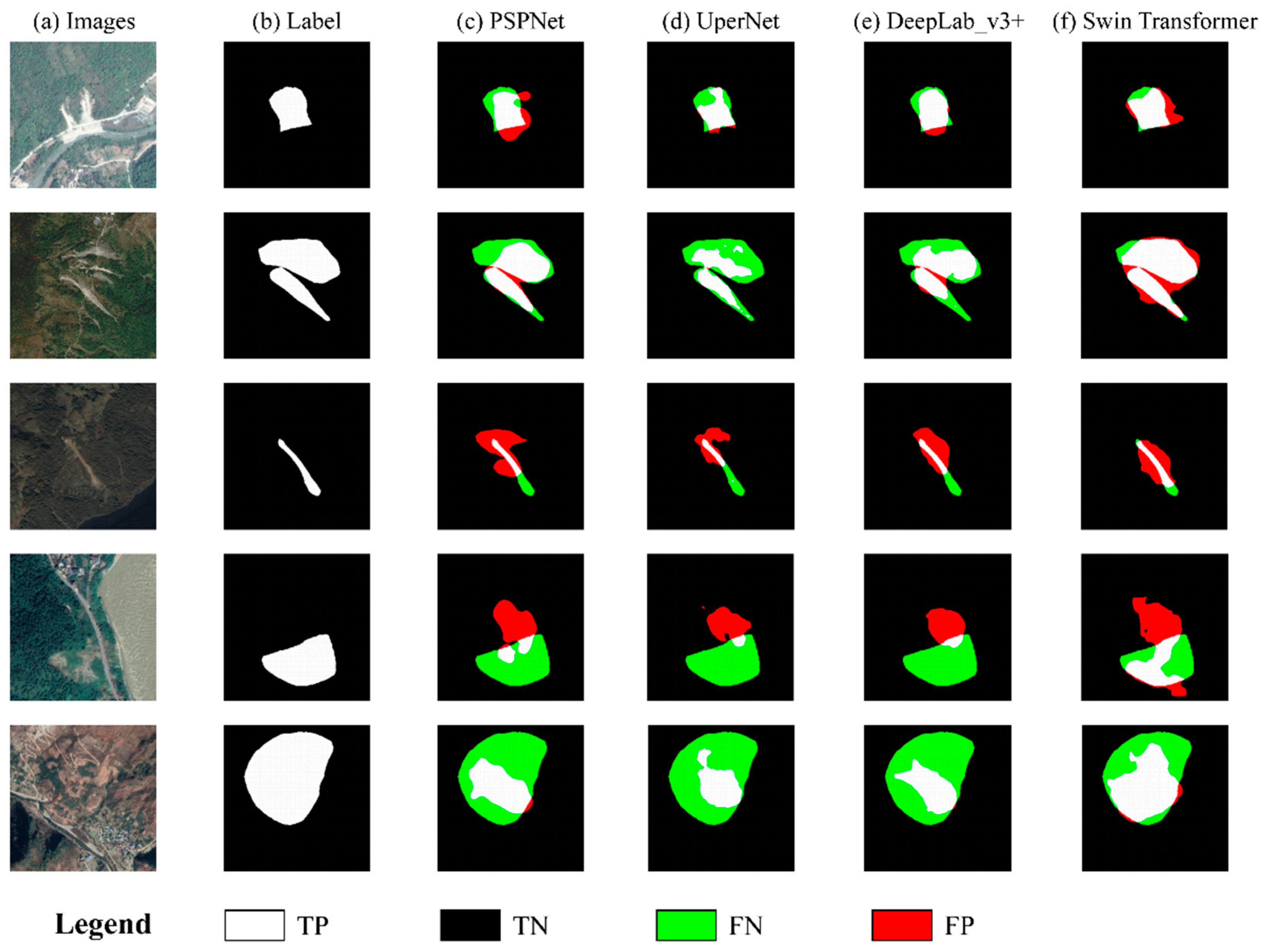
The Swin transformer-based model obtained better results in terms of the recognition of landslide disasters in Ya’an City. We randomly selected the results of image recognition using the above models in the testing dataset for comparison, as shown in Figure 12a–f, which show the original image, the labeled image, and the prediction results obtained with PSPNet, UPerNet, DeepLab_v3+, and the Swin transformer-based model, respectively.
As observed in Figure 12c–f, the Swin transformer-based model obtained the best results in terms of recognizing landslides. Even for the last row, which shows ancient landslide images, it was still the best model. PSPNet captures contextual information at different scales using the pyramid pooling module (PPM), but its core is still based on the architecture of a CNN, which may have some limitations in processing global information. Landslide phenomena are diverse—that is, they have different shapes, sizes, and contexts—and UPerNet may encounter difficulties in processing such complex image data, namely, misidentifying non-landslide areas as landslide areas or failing to recognize landslide areas in the image. DeepLab_v3+ is based on the encoder–decoder architecture, enhancing the encoder’s ability to extract semantic information through the use of an ASPP module. However, compared with the Swin transformer, it may be slightly insufficient in processing high-resolution images and capturing complex contextual relationships. In summary, the reasons that the Swin transformer-based model outperformed UPerNet, PSPNet, and DeepLab_v3+ in terms of landslide recognition accuracy are mainly its unique model design, adaptability to visual tasks, and high performance, as demonstrated in several experiments. These advantages enable the Swin transformer-based model to capture semantic information in an image more accurately when dealing with complex visual tasks such as landslide recognition, thus achieving higher recognition accuracy.

4.2.2. Network Comparison Experiments after Adding DEM Features

In complex tasks such as landslide identification, non-landslide image samples often present textures and shapes that are similar to those of landslide areas, and these interfering factors greatly increase the risk of misclassification when relying only on optical images for landslide identification [52]. However, the rich topographic information contained in digital elevation models, such as elevation changes, can provide valuable information that is complementary to optical imagery, which can help the network model to more accurately recognize landslide areas. In order to verify the practical value of using DEMs in landslide identification tasks, we explored improvements in the landslide identification performance of the network model after adding DEM data through comparative experiments. As shown in Table 3, when we trained and tested the network containing the DEM data as the fourth channel of the optical image co-input, the four network models were significantly improved with respect to the testing set in terms of all four main metrics. Among them, the OA, F1-score, IoU, and R of UPerNet were improved by 0.7%, 6.3%, 7%, and 11.8%, respectively; the F1-score, IoU, and R of PSPNet were improved by 2.8%, 2.9%, and 6.2%, respectively; the OA, F1-score, IoU, P, and R of DeepLab_v3+ were improved by 0.6%, 2.4%, 0.6%, and 9.9%, respectively; the OA, F1-score, IoU, and P of the Swin transformer-based model were improved by 1.2%, 5.2%, and 6.2%, respectively. As shown in Table 3, when we input the DEM data as the fourth channel of the optical image into the network for training and testing, based on the testing set, the four main indices of the four network models were significantly improved.
First, DEM data provide rich topographic information, which plays a crucial role in landslide identification. As a surface deformation phenomenon, the occurrence of a landslide is often closely related to topographic conditions [53]. By fusing DEM data, the deep learning model is able to learn more spatial features related to landslides and, thus, can more accurately identify landslide areas. Second, the DEM data, as a stable information source, are not affected by factors such as light conditions and vegetation cover and can provide more reliable and stable inputs for the model. In optical remote sensing imagery, changes in the lighting conditions may lead to the degradation of the image quality, affecting the recognition performance of the model. The interference of vegetation cover may also make it difficult to accurately recognize landslide areas. By incorporating DEM data, the model is able to maintain a high recognition accuracy under different environmental conditions, improving the robustness and generalization ability of the model. In addition, DEM data can provide additional contextual information to the model, which allows it to better understand the relationship between the landslide area and the surrounding environment. In landslide identification tasks, contextual information often has a significant impact on the model’s judgment. By fusing DEM data, the model is able to gain a more comprehensive understanding of topographic features, surrounding geomorphology, and possible geologic conditions of the landslide area in order to more accurately determine whether an area is a landslide area or not. The experimental results provided in Table 3 indicate that the UPerNet, PSPNet, DeepLabv3+, and Swin transformer-based deep learning models obtained significantly better values for all metrics (e.g., accuracy, recall, F1-score) in the landslide identification task when DEM data were used as an additional input channel in combination with optical remote sensing images. This fully demonstrates the important role and value of DEM data in the landslide recognition task. This is mainly due to the rich terrain information provided by DEM data, which is characterized by a stable information source, additional contextual information, and complementarity with other input information.

4.2.3. Optimization Experiments Using Boundary Loss Functions

In a landslide dataset, the landslide samples (positive classes) tend to make up only a small portion of the entire dataset, while the non-landslide samples (negative classes) make up the vast majority. This imbalance causes the model to be more likely to favor the majority class (i.e., non-landslide samples) during the training process, as the majority class contains a large number of samples, and it is easier for the model to reduce the loss of the majority class during the optimization process. This can have a significant impact on the model’s learning ability, resulting in a decrease in the overall recognition accuracy of the model. Although the prediction accuracy of the Swin transformer-based model was better compared to classical networks, this model still has some room for improvement. When dealing with extremely unbalanced classification tasks such as the considered landslide dataset, the introduction of the boundary loss function (BLF) can improve the performance of the Swin transformer, which relies only on the binary cross-entropy function. The changes in the specific evaluation indices are shown in Table 4. When the Swin transformer-based model was trained using optical images and the boundary loss function was added, the OA, F1-score, IoU, and R of the model improved by 0.6%, 0.5%, 0.5%, and 8.2%, respectively. When the optical images and DEM data were fused using the Swin transformer and the boundary loss function was added, the OA, F1-score, IoU, and R of the model improved by 0.2%, 0.9%, 1.2%, and 2.2%, respectively.
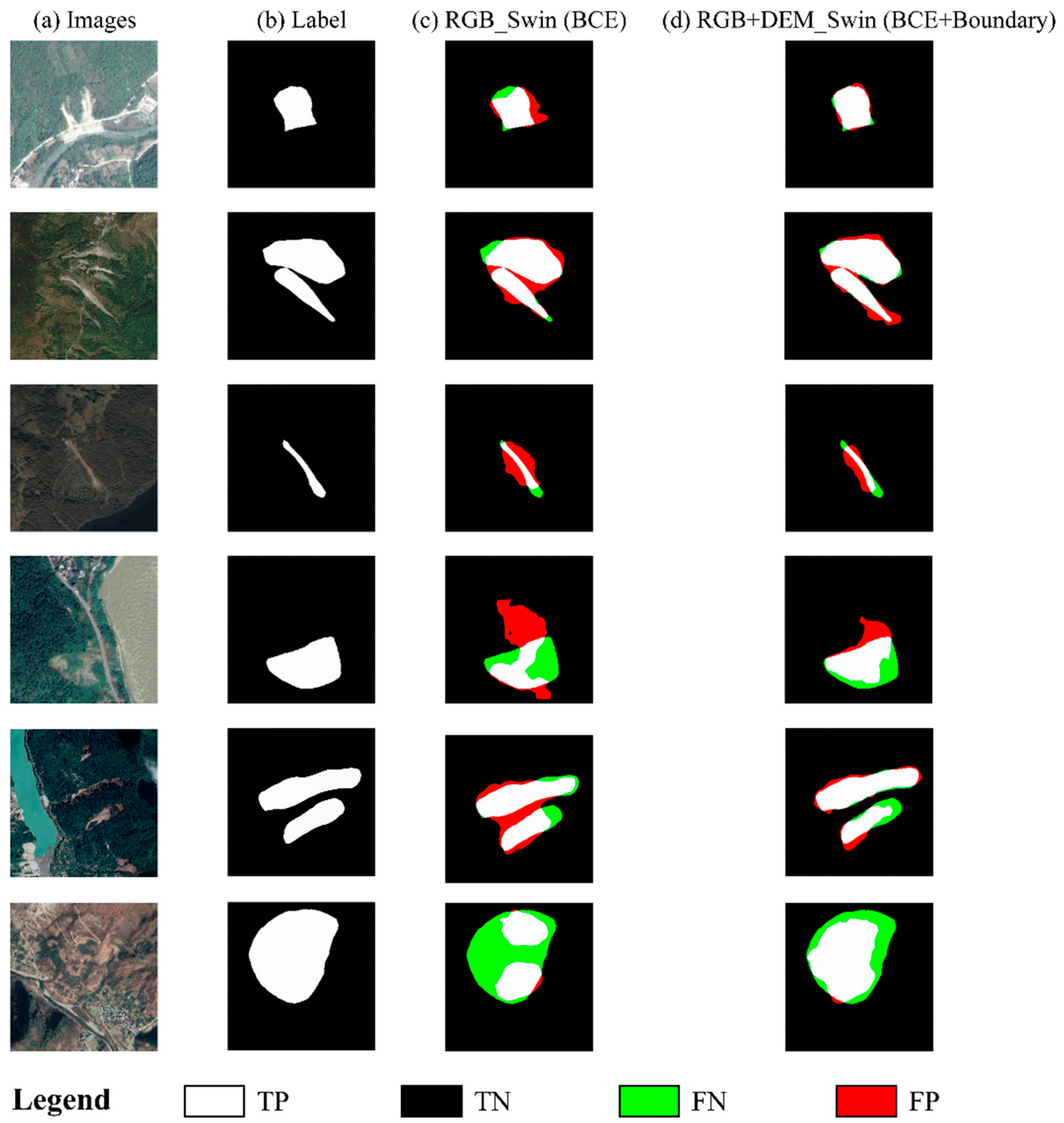
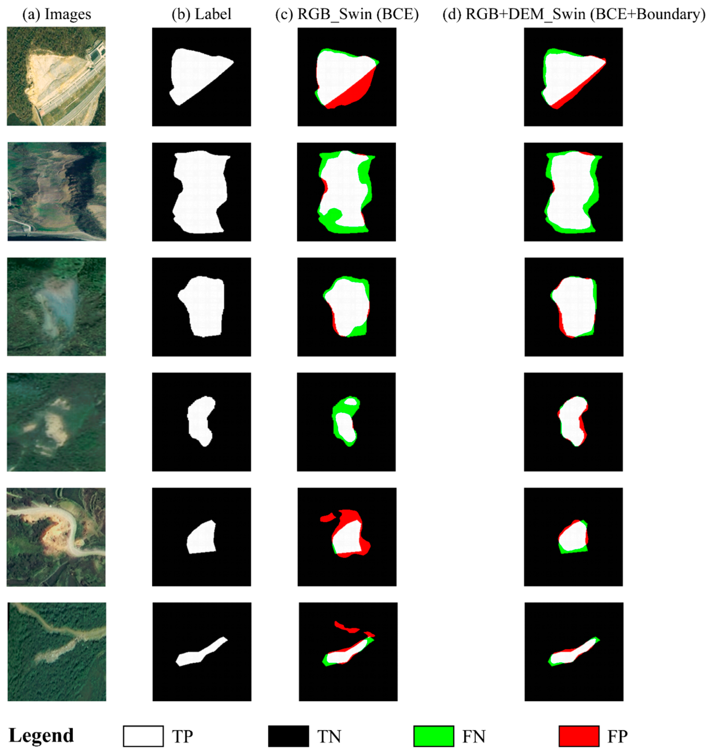
Compared with the Swin transformer-based model using only optical images as input, the accuracy evaluation indices were significantly improved when fusing elevation information and introducing the boundary loss function; in particular, the OA, F1-score, IoU, and P of the model improved by 1.4%, 6.3%, 7.7%, and 12.4%, respectively. In order to visually compare the degree of optimization of the prediction results with the introduction of the boundary loss function, the recognition image results with respect to the testing dataset were selected. The results of the comparison are shown in Figure 13a–d, which show the original image, the labeled image, the Swin transformer-based model trained on the optical images (this model uses the binary cross-entropy function), and the Swin transformer-based model trained on optical images and DEM data (this model uses the binary cross-entropy function and boundary loss function).
When dealing with landslide datasets, particularly when the landslide areas are closely adjacent and difficult to distinguish, traditional identification models are often challenged and may incorrectly identify two landslides that are in close proximity to each other as one large landslide. Before the introduction of the boundary loss function, it was difficult for the model to accurately capture subtle differences between landslides due to the unbalanced nature of the dataset and the fuzzy boundaries between the landslide regions. A consequence of this was that neighboring landslides that were very close to one another could be mistakenly recognized as the same landslide during the classification process and, thus, were merged into one landslide during identification.
However, by introducing a boundary loss function, the model is able to focus more attention on the samples near the classification boundary, especially regions located between neighboring landslides. The design of the boundary loss function allows the model to give special consideration to these boundary samples during the optimization process, and it attempts to create a clearer demarcation between them. This strategy allows the model to more accurately identify the boundaries between neighboring landslides, thus avoiding incorrect merging into one large landslide. Landslide samples usually account for a relatively small proportion of the dataset; this results in the phenomenon in which traditional models become easily biased towards the non-landslide samples (i.e., the majority class) during the training process, thus failing to accurately identify landslide samples (i.e., the minority class). The introduction of the boundary loss function not only helps the model pay more attention to the samples near the classification boundary—especially the landslide and non-landslide samples that are difficult to distinguish—but also improves the sensitivity of the model to landslide samples. This strategy not only helps improve the model’s recognition accuracy relative to the landslide samples, but, more importantly, it can also influence the model in carrying out more refined recognition during the classification process. By suppressing the risk of misclassifying samples and optimizing the model’s decision-making at the classification boundary, the boundary loss function helps achieve the precise classification of landslide samples, thus improving the overall landslide detection and identification accuracy and providing more reliable technical support for the early warning and prevention of geological disasters.

5. Discussion

5.1. Interpretation of the Models’ Visualization Results

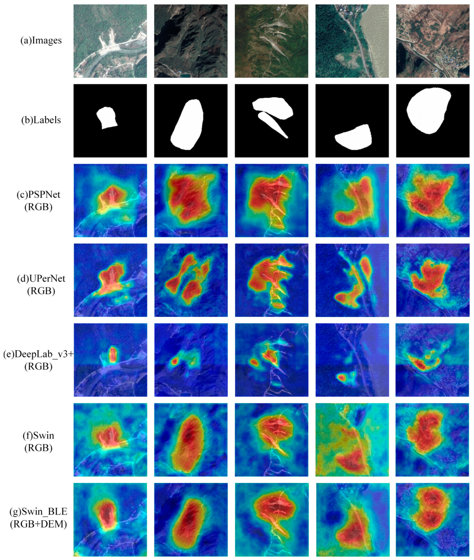
In order to obtain the part of the image that contributes the most to the output category and improve the accuracy of the feature matching during image retrieval, we introduce the heat map for intuition and visualization purposes. We mapped the extracted feature data to the corresponding locations on the map to form a preliminary spatial distribution map. Different colors are assigned to each region of the image based on the values of the feature data (predicted probability values for the testing set) in order to create a heatmap. In the heatmap, red indicates high-risk areas, while blue indicates low-risk areas. In this paper, we use heatmaps to compare the intelligent identification results of the optimal Swin transformer-based model to the benchmark network without fused DEM features, which can visualize the prediction ability of the Swin transformer-based model. As shown in Figure 14, the feature fusion enhancement allowed the Swin transformer-based model to more accurately identify landslide areas during prediction. The areas with very high and very low landslide risks are shown in dark red and dark blue, respectively, on the heat map; specifically, the dark red areas represent areas with a high probability of landslide identification, while the dark blue areas represent areas with a low probability of landslide identification. This process of feature fusion directly results in a reduction in the transition colors, as the model may have learned to predict landslide areas more directly and accurately.
Optical images and DEM data each have unique information characteristics. Optical images mainly record the spectral information and texture characteristics of the ground surface, which can reflect intuitive information, such as the vegetation cover and soil type. Meanwhile, DEM data provide three-dimensional information about the terrain, which is crucial for understanding the occurrence mechanism of geohazards. Therefore, the fusion of these two data features can fully leverage the complementarity between them, enabling the model to capture more comprehensive and accurate landslide-related features. The Swin transformer, as a deep learning model based on the Transformer architecture, has a powerful feature extraction capability. In the feature extraction stage, the model is able to gradually fuse the features of the optical image and DEM through multi-layer convolution and pooling operations. This fusion process not only superimposes the features of the two datasets, but also further enhances the key features related to landslide occurrence through operations such as non-linear transformation and feature selection. The effects of this feature enhancement allowed the model to identify landslide areas more accurately during prediction and to refine the prediction results.

5.2. Model Resilience Analysis Based on a Publicly Available Landslide Dataset

In the field of landslide hazard prediction and prevention, the adaptability of a model is one of the most important indicators of its performance. In order to fully evaluate the effectiveness of our selected and modified models for practical applications, we conducted a test on a publicly available landslide dataset [54] of Bijie City, Guizhou Province, China.
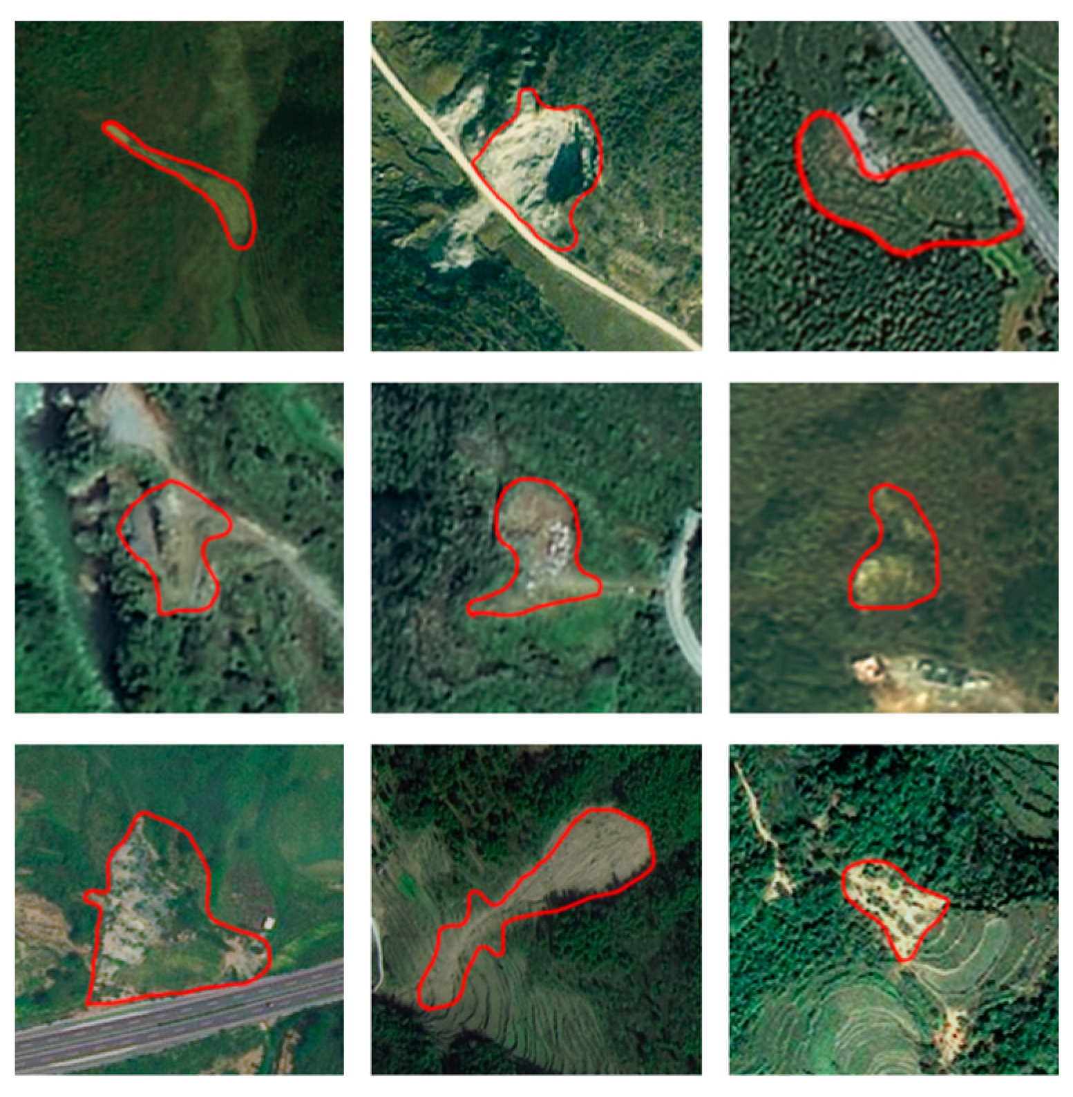
Bijie City is located in the northwestern part of Guizhou Province, and it is characterized by complex geological conditions and frequent landslide disasters. The considered dataset comprises data related to 770 landslide events in Bijie City, including labeled information such as the extent and size of the landslides; high-resolution optical satellite imagery, which visualizes the textural characteristics of the landslides; and elevation data, which provide key information for understanding the topographic and geomorphic conditions under which the landslides occurred. Examples of the landslides are shown in Figure 15.
During the experiment, four benchmark networks (UPerNet, PSPNet, DeepLab_v3+, and the Swin transformer-based model), as mentioned above, were selected for testing. According to the pre-determined experimental scheme, the data in the Bijie landslide dataset were randomly divided into training, validation, and test sets, and data enhancement was performed on the training set samples. To ensure the fairness and accuracy of the experiments, these networks were not re-trained, but the optimal weights for each previously trained model were directly used. The initial performance evaluation of the models loaded with optimal weights was performed using the validation set’s data in order to ensure that the best model was used. The results of the model testing are detailed in Table 5.
From the above table, it can be observed that the model accuracy performed better overall after loading the optimal weights from previous training. This is because the pre-training weights were obtained through previous training on a dataset; thus, the model had already learned a rich feature representation. When these weights were used to initialize a new task, they were able to take advantage of the already learned knowledge, exhibiting high initial landslide recognition accuracy with respect to Bijie data. Meanwhile, the effectiveness of the pre-training weights depends to a large extent on the relevance of the pre-training task to the target task. As all landslides were targeted in this study, the improvement introduced by previous pre-training weights was more significant. After adding DEM data, the overall performance of the models showed an upward trend, which is sufficient to conclude that the DEM data provide more dimensional information for the model, thus helping the model to understand landslide phenomena more comprehensively.
The Swin transformer-based model effectively handles high-resolution images through its hierarchical structure, windowed self-attention mechanism, and shifted window technique, and it achieved excellent landslide recognition performance with respect to the Bijie dataset. In order to improve the recognition accuracy of the model, it was chosen to utilize the boundary constraint function such that the final prediction results were more in line with a priori knowledge. The obtained evaluation indices are provided in Table 6.
The experimental results show that all accuracy indices of the model were improved after adding the boundary constraint function, which further verifies the effectiveness of the boundary constraint function in improving the performance of the model. Compared to the Swin transformer-based model with only optical images as input, the accuracy evaluation index of the Swin transformer-based model was significantly improved after fusing the elevation information and introducing the boundary loss function. The OA, F1 score, IoU, and PA of the model were improved by 0.8%, 3.2%, 4.8%, and 6%, respectively. In order to visually compare the optimization degree of the prediction results after the introduction of the boundary loss function, the results for certain images in the Bijie test dataset were selected, as shown in Figure 16. Figure 16a–d show the original image, labeled image, the Swin transformer-based model’s prediction results when trained on optical images (using the binary cross-entropy function), and the prediction results when the model was trained on optical images and DEM data (using the binary cross-entropy function and a boundary loss function). When the elevation information was combined with the boundary constraint function, they complemented each other and jointly enhanced the recognition effect of the model. Elevation information can be combined with other image features (e.g., color, texture) to form a richer and more accurate feature representation. This multi-dimensional feature representation helps the model better capture the essential features of the target object, thus improving the recognition effect. The boundary constraint function, on the other hand, further improves the recognition accuracy of the model by introducing prior knowledge and optimizing the decision boundary. This combination makes the model more accurate and efficient in dealing with targets with significant elevation features.

5.3. Comparison of Model Recognition Performance for Different Datasets

In the field of landslide identification, the diversity and complexity of datasets pose a serious challenge to model performance [55,56]. In this study, four deep learning models—Swin transformer, UPerNet, PSPNet, and DeepLab_v3+—were applied for landslide recognition experiments for the Ya’an and Bijie datasets, respectively. With respect to the two different datasets, the Swin transformer model superimposed on the boundary loss function exhibited optimal recognition performance, while the UPerNet, PSPNet, and DeepLab_v3+ models performed slightly worse. Both the Ya’an dataset and the Bijie dataset contain elevation data and optical imagery, which provide rich information on topographic landforms and texture features for landslide identification. Elevation data [57] provide information on the elevation of the terrain, which helps identify changes in the terrain, such as ground subsidence or uplift caused by landslides, while optical imagery [58] provides information on the ground cover and texture, which helps identify features such as vegetation damage, cracks, etc., in landslide areas. Moreover, the landslide types in both datasets cover both recent landslides and deformed slopes, which further increases the complexity of the identification task. Recent landslides are usually characterized by more obvious surface deformation and cracks [59], while deformed slopes [60] may show minor ground surface deformations or changes in vegetation cover, and high-precision feature extraction and recognition capabilities for accurate judgment are needed.
The optimized Swin transformer model exhibited the best recognition results relative to both datasets, and this is mainly due to its powerful feature extraction capability and adaptability to complex scenes. The model is able to effectively capture key features of the landslide region, such as topographic changes, crack distribution, and differences in vegetation cover, through the self-attention mechanism and window delineation strategy. Simultaneously, the Swin transformer is able to take full advantage of the complementary information of these two data sources when processing complex datasets containing both DEM data and optical imagery to achieve more accurate landslide identification. The boundary loss function plays an important role in landslide identification tasks. The boundaries between landslide and non-landslide areas are often irregular, and they are affected by a variety of factors, such as topography, vegetation, and rainfall. This makes it challenging for the model to determine the boundary. The boundary loss function, however, optimizes the decision boundary of the model by increasing the focus on the samples near the classification boundary. When the model’s prediction of the boundary samples does not match the true labels, the boundary loss function exhibits a large penalty, prompting the model to adjust its parameters to better fit the true classification boundary. This mechanism helps improve the model’s ability to recognize boundary samples, resulting in more accurate results for landslide identification.
In contrast, the UPerNet, PSPNet, and DeepLab_v3+ models show some limitations when dealing with these complex scenarios. Although these models have achieved good results in their respective areas of expertise, there is still more room for performance improvement when facing the specific task of landslide identification. This may be related to the strategies of these models in feature extraction, contextual information fusion, and multi-scale processing. We can make improvements with respect to the following: first, the model’s adaptive training can be strengthened relative to complex scenes, and the model’s sensitivity to key features, such as terrain changes and crack distribution, can be improved; second, the model’s contextual information fusion strategy should be modified, and complementary information relative to DEM data and optical imagery should be made use of; third, a multi-scale feature extraction and processing mechanism should be introduced in order to improve the model’s recognition of landslide targets at different scales.

6. Conclusions

This study focused on Ya’an City, a landslide-prone area in the Sichuan Basin. We collected geological, environmental, and optical imagery data. Using remote sensing and AI, we addressed the challenge of landslide identification, a small-sample learning problem. We employed a Swin transformer-based model to enhance recognition accuracy by integrating optical images and DEM data. The introduction of a boundary constraint function further refined the results compared to classical networks (PSPNet, UPerNet, and DeepLab_V3+). The key findings include the following.
The performance of the original Swin transformer-based model, relying solely on the binary cross-entropy function, was significantly enhanced by incorporating the boundary loss function. Compared to only using optical images, the model’s accuracy evaluation indices, including OA, F1-score, IoU, and P, were improved by 1.4%, 6.3%, 7.7%, and 12.4%, respectively, when integrating DEM information and using the boundary loss function.
Testing using the landslide dataset of Bijie City, Guizhou Province, to verify the model’s resilience revealed that adding pre-training weights enhanced the performance. With the inclusion of elevation information and the boundary constraint function, the Swin transformer-based model’s OA, F1 score, IoU, and PA improved by 0.8%, 3.2%, 4.8%, and 6% respectively, compared to only using optical images. This demonstrated that combining elevation information and the boundary constraint function further boosted the model’s recognition ability.
However, this study has limitations. Firstly, the model’s generalization ability may be impacted by the study area and sample size constraints. To validate its applicability, future tests in diverse geological and environmental conditions are necessary. Secondly, while the Swin transformer exhibited remarkable results with respect to landslide identification, its computational complexity is high, and the model size is large, posing challenges for real-time performance and computational resources in practical applications. Exploring lightweight and efficient model architectures is a crucial direction for future research.

Author Contributions

Conceptualization, X.W., S.C. and D.W.; methodology, X.W., W.L. and J.D.; software, D.W. and L.X.; validation, T.S. and J.D.; formal analysis, C.L.; investigation, X.W.; resources, D.W.; data curation, X.W.; writing—original draft preparation, X.W. and M.Z.; writing—review and editing, M.Z.; visualization X.W.; supervision, X.W.; project administration, X.W.; funding acquisition, L.X. All authors have read and agreed to the published version of the manuscript.

Funding

This research was funded by the National Natural Science Foundation of China, grant number 52208006, and the Technology Innovation Center for Geological Disaster Prevention and Ecological Restoration in Western China, MNR (Chengdu University of Technology), grant number TICGP2023K002.

Data Availability Statement

The original contributions presented in the study are included in the article, further inquiries can be directed to the corresponding author.

Acknowledgments

We thank LetPub (www.letpub.com) for its linguistic assistance during the preparation of this manuscript.

Conflicts of Interest

Author Tiegang Sun was employed by the company China Building Materials Southwest Survey and Design Co., Ltd. The remaining authors declare that the research was conducted in the absence of any commercial or financial relationships that could be construed as a potential conflict of interest.

References

  1. Zhao, Z.; Lan, H.; Li, L.; Strom, A. Landslide Spatial Prediction Using Cluster Analysis. Gondwana Res. 2024, 130, 291–307. [Google Scholar] [CrossRef]
  2. Chen, X.; Chen, W. GIS-Based Landslide Susceptibility Assessment Using Optimized Hybrid Machine Learning Methods. Catena 2021, 196, 104833. [Google Scholar] [CrossRef]
  3. Bui, D.T.; Tsangaratos, P.; Nguyen, V.-T.; Van Liem, N.; Trinh, P.T. Comparing the Prediction Performance of a Deep Learning Neural Network Model with Conventional Machine Learning Models in Landslide Susceptibility Assessment. Catena 2020, 188, 104426. [Google Scholar] [CrossRef]
  4. Yang, C.; Liu, L.-L.; Huang, F.; Huang, L.; Wang, X.-M. Machine Learning-Based Landslide Susceptibility Assessment with Optimized Ratio of Landslide to Non-Landslide Samples. Gondwana Res. 2023, 123, 198–216. [Google Scholar] [CrossRef]
  5. Cheng, G.; Wang, Z.; Huang, C.; Yang, Y.; Hu, J.; Yan, X.; Tan, Y.; Liao, L.; Zhou, X.; Li, Y.; et al. Advances in Deep Learning Recognition of Landslides Based on Remote Sensing Images. Remote Sens. 2024, 16, 1787. [Google Scholar] [CrossRef]
  6. Xu, Y.; Ouyang, C.; Xu, Q.; Wang, D.; Zhao, B.; Luo, Y. CAS Landslide Dataset: A Large-Scale and Multisensor Dataset for Deep Learning-Based Landslide Detection. Sci. Data 2024, 11, 12. [Google Scholar] [CrossRef]
  7. Ju, Y.; Xu, Q.; Jin, S.; Li, W.; Su, Y.; Dong, X.; Guo, Q. Loess Landslide Detection Using Object Detection Algorithms in Northwest China. Remote Sens. 2022, 14, 1182. [Google Scholar] [CrossRef]
  8. Ma, L.; Liu, Y.; Zhang, X.; Ye, Y.; Yin, G.; Johnson, B.A. Deep Learning in Remote Sensing Applications: A Meta-Analysis and Review. ISPRS J. Photogramm. Remote Sens. 2019, 152, 166–177. [Google Scholar] [CrossRef]
  9. Audebert, N.; Le Saux, B.; Lefèvre, S. Semantic Segmentation of Earth Observation Data Using Multimodal and Multi-Scale Deep Networks. In Proceedings of the Asian Conference on Computer Vision, Taipei, Taiwan, 20–24 November 2016; Springer: Berlin/Heidelberg, Germany, 2016; pp. 180–196. [Google Scholar]
  10. Tao, A.; Sapra, K.; Catanzaro, B. Hierarchical Multi-Scale Attention for Semantic Segmentation. arXiv 2020, arXiv:2005.10821. [Google Scholar]
  11. Hoyer, L.; Dai, D.; Van Gool, L. Daformer: Improving Network Architectures and Training Strategies for Domain-Adaptive Semantic Segmentation. In Proceedings of the IEEE/CVF Conference on Computer Vision and Pattern Recognition, New Orleans, LA, USA, 18–24 June 2022; pp. 9924–9935. [Google Scholar]
  12. He, H.; Cai, J.; Pan, Z.; Liu, J.; Zhang, J.; Tao, D.; Zhuang, B. Dynamic Focus-Aware Positional Queries for Semantic Segmentation. In Proceedings of the IEEE/CVF Conference on Computer Vision and Pattern Recognition, Vancouver, BC, Canada, 17–24 June 2023; pp. 11299–11308. [Google Scholar]
  13. Nguyen, T.; Nguyen, L.; Tran, P.; Nguyen, H. Improving Transformer-Based Neural Machine Translation with Prior Alignments. Complexity 2021, 2021, 5515407. [Google Scholar] [CrossRef]
  14. Liu, Z.; Lin, Y.; Cao, Y.; Hu, H.; Wei, Y.; Zhang, Z.; Lin, S.; Guo, B. Swin Transformer: Hierarchical Vision Transformer Using Shifted Windows. In Proceedings of the IEEE/CVF International Conference on Computer Vision, Montreal, BC, Canada, 11–17 October 2021; pp. 10012–10022. [Google Scholar]
  15. Pourghasemi, H.R.; Sadhasivam, N.; Amiri, M.; Eskandari, S.; Santosh, M. Landslide Susceptibility Assessment and Mapping Using State-of-the Art Machine Learning Techniques. Nat. Hazards 2021, 108, 1291–1316. [Google Scholar] [CrossRef]
  16. Lee, S.I.; Koo, K.; Lee, J.H.; Lee, G.; Jeong, S.; O, S.; Kim, H. Vision Transformer Models for Mobile/Edge Devices: A Survey. Multimed Syst. 2024, 30, 109. [Google Scholar] [CrossRef]
  17. Liu, Y.; Nand, P.; Hossain, M.A.; Nguyen, M.; Yan, W.Q. Sign Language Recognition from Digital Videos Using Feature Pyramid Network with Detection Transformer. Multimed. Tools Appl. 2023, 82, 21673–21685. [Google Scholar] [CrossRef]
  18. Dong, Z.; Wang, Q.; Zhu, P. Multi-Head Second-Order Pooling for Graph Transformer Networks. Pattern Recognit. Lett. 2023, 167, 53–59. [Google Scholar] [CrossRef]
  19. Nie, J.; Xie, J.; Sun, H. Remote Sensing Image Dehazing via a Local Context-Enriched Transformer. Remote Sens. 2024, 16, 1422. [Google Scholar] [CrossRef]
  20. Pacal, I.; Alaftekin, M.; Zengul, F.D. Enhancing Skin Cancer Diagnosis Using Swin Transformer with Hybrid Shifted Window-Based Multi-Head Self-Attention and SwiGLU-Based MLP. J. Imaging Inform. Med. 2024, 1–19. [Google Scholar] [CrossRef]
  21. Kim, H.; Yim, C. Swin Transformer Fusion Network for Image Quality Assessment. IEEE Access 2024, 12, 57741–57754. [Google Scholar] [CrossRef]
  22. Zhong, F.; He, K.; Ji, M.; Chen, J.; Gao, T.; Li, S.; Zhang, J.; Li, C. Optimizing Vitiligo Diagnosis with ResNet and Swin Transformer Deep Learning Models: A Study on Performance and Interpretability. Sci. Rep. 2024, 14, 9127. [Google Scholar] [CrossRef]
  23. Liu, E.; He, B.; Zhu, D.; Chen, Y.; Xu, Z. Tiny Polyp Detection from Endoscopic Video Frames Using Vision Transformers. Pattern Anal. Appl. 2024, 27, 38. [Google Scholar] [CrossRef]
  24. Ramkumar, K.; Medeiros, E.P.; Dong, A.; de Albuquerque, V.H.C.; Hassan, M.R.; Hassan, M.M. A Novel Deep Learning Framework Based Swin Transformer for Dermal Cancer Cell Classification. Eng. Appl. Artif. Intell. 2024, 133, 108097. [Google Scholar] [CrossRef]
  25. Pacal, I. A Novel Swin Transformer Approach Utilizing Residual Multi-Layer Perceptron for Diagnosing Brain Tumors in MRI Images. Int. J. Mach. Learn. Cybern. 2024, 15, 3579–3597. [Google Scholar] [CrossRef]
  26. Dai, Y.; Liu, F.; Chen, W.; Liu, Y.; Shi, L.; Liu, S.; Zhou, Y. Swin MAE: Masked Autoencoders for Small Datasets. Comput. Biol. Med. 2023, 161, 107037. [Google Scholar]
  27. Masood, A.; Naseem, U.; Kim, J. Multi-Level Swin Transformer Enabled Automatic Segmentation and Classification of Breast Metastases. In Proceedings of the 2023 45th Annual International Conference of the IEEE Engineering in Medicine & Biology Society (EMBC), Sydney Australia, 24–27 July 2023; IEEE: Piscataway, NJ, USA, 2023; pp. 1–4. [Google Scholar]
  28. Guo, Z.; He, Z.; Lyu, L.; Mao, A.; Huang, E.; Liu, K. Automatic Detection of Feral Pigeons in Urban Environments Using Deep Learning. Animals 2024, 14, 159. [Google Scholar] [CrossRef]
  29. Gao, L.; Zhang, J.; Yang, C.; Zhou, Y. Cas-VSwin Transformer: A Variant Swin Transformer for Surface-Defect Detection. Comput. Ind. 2022, 140, 103689. [Google Scholar] [CrossRef]
  30. Yuan, W.; Xu, W. Neighborloss: A Loss Function Considering Spatial Correlation for Semantic Segmentation of Remote Sensing Image. IEEE Access 2021, 9, 75641–75649. [Google Scholar] [CrossRef]
  31. Yeung, M.; Sala, E.; Schönlieb, C.-B.; Rundo, L. Unified Focal Loss: Generalising Dice and Cross Entropy-Based Losses to Handle Class Imbalanced Medical Image Segmentation. Comput. Med. Imaging Graph. 2022, 95, 102026. [Google Scholar] [CrossRef]
  32. Guo, Q.; Wang, C.; Xiao, D.; Huang, Q. A Novel Multi-Label Pest Image Classifier Using the Modified Swin Transformer and Soft Binary Cross Entropy Loss. Eng. Appl. Artif. Intell. 2023, 126, 107060. [Google Scholar] [CrossRef]
  33. Agarwal, N.; Balasubramanian, V.N.; Jawahar, C.V. Improving Multiclass Classification by Deep Networks Using DAGSVM and Triplet Loss. Pattern Recognit. Lett. 2018, 112, 184–190. [Google Scholar] [CrossRef]
  34. Xiang, S.; Liang, Q.; Hu, Y.; Tang, P.; Coppola, G.; Zhang, D.; Sun, W. AMC-Net: Asymmetric and Multi-Scale Convolutional Neural Network for Multi-Label HPA Classification. Comput. Methods Programs Biomed. 2019, 178, 275–287. [Google Scholar] [CrossRef] [PubMed]
  35. Zhang, H.; Qian, Z.; Tan, Y.; Xie, Y.; Li, M. Investigation of Pavement Crack Detection Based on Deep Learning Method Using Weakly Supervised Instance Segmentation Framework. Constr. Build. Mater. 2022, 358, 129117. [Google Scholar] [CrossRef]
  36. Zhang, M.; Wang, H.; Wang, L.; Saif, A.; Wassan, S. CIDN: A Context Interactive Deep Network with Edge-Aware for X-Ray Angiography Images Segmentation. Alex. Eng. J. 2024, 87, 201–212. [Google Scholar] [CrossRef]
  37. Pawara, P.; Okafor, E.; Groefsema, M.; He, S.; Schomaker, L.R.B.; Wiering, M.A. One-vs-One Classification for Deep Neural Networks. Pattern Recognit. 2020, 108, 107528. [Google Scholar] [CrossRef]
  38. Wang, P.; Chung, A.C.S. Relax and Focus on Brain Tumor Segmentation. Med. Image Anal. 2022, 75, 102259. [Google Scholar] [CrossRef]
  39. Wang, G.; Wang, F.; Zhou, H.; Lin, H. Fire in Focus: Advancing Wildfire Image Segmentation by Focusing on Fire Edges. Forests 2024, 15, 217. [Google Scholar] [CrossRef]
  40. Ma, J.; Liang, P.; Yu, W.; Chen, C.; Guo, X.; Wu, J.; Jiang, J. Infrared and Visible Image Fusion via Detail Preserving Adversarial Learning. Inf. Fusion 2020, 54, 85–98. [Google Scholar] [CrossRef]
  41. Zhai, J.; Mu, C.; Hou, Y.; Wang, J.; Wang, Y.; Chi, H. A Dual Attention Encoding Network Using Gradient Profile Loss for Oil Spill Detection Based on SAR Images. Entropy 2022, 24, 1453. [Google Scholar] [CrossRef] [PubMed]
  42. Li, H.; He, Y.; Xu, Q.; Deng, J.; Li, W.; Wei, Y. Detection and Segmentation of Loess Landslides via Satellite Images: A Two-Phase Framework. Landslides 2022, 19, 673–686. [Google Scholar] [CrossRef]
  43. Zhou, Y.; Wang, H.; Yang, R.; Yao, G.; Xu, Q.; Zhang, X. A Novel Weakly Supervised Remote Sensing Landslide Semantic Segmentation Method: Combining CAM and CycleGAN Algorithms. Remote Sens. 2022, 14, 3650. [Google Scholar] [CrossRef]
  44. Feng, X.; Du, J.; Wu, M.; Chai, B.; Miao, F.; Wang, Y. Potential of Synthetic Images in Landslide Segmentation in Data-Poor Scenario: A Framework Combining GAN and Transformer Models. Landslides 2024, 21, 2211–2226. [Google Scholar] [CrossRef]
  45. Lan, H.; Liu, X.; Li, L.; Li, Q.; Tian, N.; Peng, J. Remote Sensing Precursors Analysis for Giant Landslides. Remote Sens. 2022, 14, 4399. [Google Scholar] [CrossRef]
  46. Grigoryan, A.M.; Agaian, S.S. Monotonic Sequences for Image Enhancement and Segmentation. Digit. Signal Process. 2015, 41, 70–89. [Google Scholar] [CrossRef]
  47. Liang, L.; Zhang, Z.-M. Structure-Aware Enhancement of Imaging Mass Spectrometry Data for Semantic Segmentation. Chemom. Intell. Lab. Syst. 2017, 171, 259–265. [Google Scholar] [CrossRef]
  48. Domokos, C.; Kato, Z. Parametric Estimation of Affine Deformations of Planar Shapes. Pattern Recognit. 2010, 43, 569–578. [Google Scholar] [CrossRef]
  49. Qin, Z.; Chen, Q.; Ding, Y.; Zhuang, T.; Qin, Z.; Choo, K.-K.R. Segmentation Mask and Feature Similarity Loss Guided GAN for Object-Oriented Image-to-Image Translation. Inf. Process. Manag. 2022, 59, 102926. [Google Scholar] [CrossRef]
  50. Schmitter, D.; Unser, M. Shape Projectors for Landmark-Based Spline Curves. IEEE Signal Process. Lett. 2017, 24, 1517–1521. [Google Scholar] [CrossRef]
  51. Mehrish, A.; Subramanyam, A.V.; Emmanuel, S. Sensor Pattern Noise Estimation Using Probabilistically Estimated RAW Values. IEEE Signal Process. Lett. 2016, 23, 693–697. [Google Scholar] [CrossRef]
  52. Yang, Y.; Mei, G. Deep Transfer Learning Approach for Identifying Slope Surface Cracks. Appl. Sci. 2021, 11, 11193. [Google Scholar] [CrossRef]
  53. Li, D.; Tang, X.; Tu, Z.; Fang, C.; Ju, Y. Automatic Detection of Forested Landslides: A Case Study in Jiuzhaigou County, China. Remote Sens. 2023, 15, 3850. [Google Scholar] [CrossRef]
  54. Ji, S.; Yu, D.; Shen, C.; Li, W.; Xu, Q. Landslide Detection from an Open Satellite Imagery and Digital Elevation Model Dataset Using Attention Boosted Convolutional Neural Networks. Landslides 2020, 17, 1337–1352. [Google Scholar] [CrossRef]
  55. Ma, Z.; Mei, G. Deep Learning for Geological Hazards Analysis: Data, Models, Applications, and Opportunities. Earth-Sci. Rev. 2021, 223, 103858. [Google Scholar] [CrossRef]
  56. Merghadi, A.; Yunus, A.P.; Dou, J.; Whiteley, J.; ThaiPham, B.; Bui, D.T.; Avtar, R.; Abderrahmane, B. Machine Learning Methods for Landslide Susceptibility Studies: A Comparative Overview of Algorithm Performance. Earth-Sci. Rev. 2020, 207, 103225. [Google Scholar] [CrossRef]
  57. Becek, K.; Ibrahim, K.; Bayik, C.; Abdikan, S.; Kutoglu, H.S.; Glabicki, D.; Blachowski, J. Identifying Land Subsidence Using Global Digital Elevation Models. IEEE J. Sel. Top. Appl. Earth Obs. Remote Sens. 2021, 14, 8989–8998. [Google Scholar] [CrossRef]
  58. Zhong, C.; Liu, Y.; Gao, P.; Chen, W.; Li, H.; Hou, Y.; Nuremanguli, T.; Ma, H. Landslide Mapping with Remote Sensing: Challenges and Opportunities. Int. J. Remote Sens. 2020, 41, 1555–1581. [Google Scholar] [CrossRef]
  59. Lian, X.-G.; Li, Z.-J.; Yuan, H.-Y.; Liu, J.-B.; Zhang, Y.-J.; Liu, X.-Y.; Wu, Y.-R. Rapid Identification of Landslide, Collapse and Crack Based on Low-Altitude Remote Sensing Image of UAV. J. Mt. Sci. 2020, 17, 2915–2928. [Google Scholar] [CrossRef]
  60. Wasowski, J.; Bovenga, F. Investigating Landslides and Unstable Slopes with Satellite Multi Temporal Interferometry: Current Issues and Future Perspectives. Eng. Geol. 2014, 174, 103–138. [Google Scholar] [CrossRef]
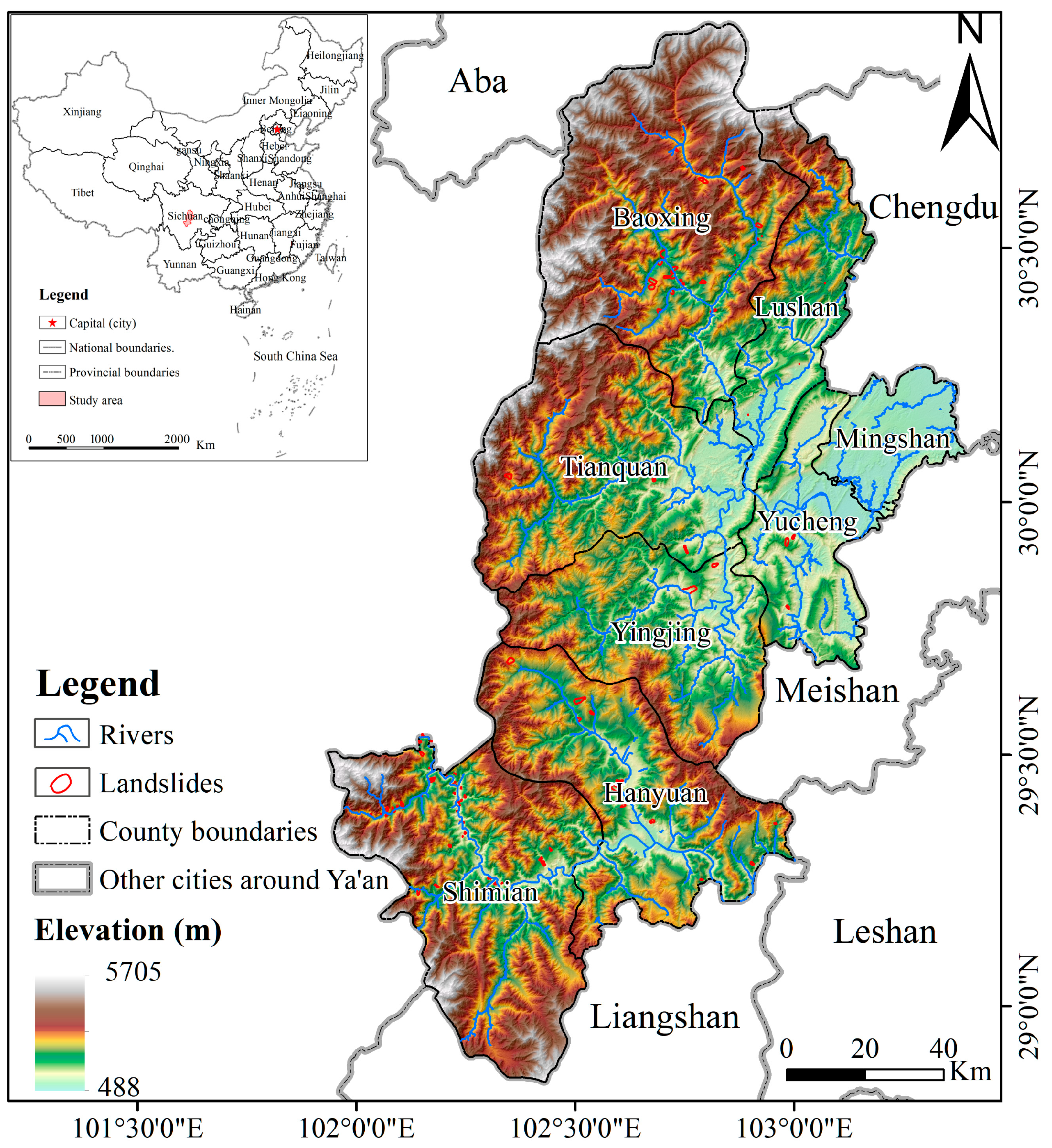
Figure 1. Distribution of landslides in Ya’an (2021–2023).
Remotesensing 16 03119 g001
Figure 2. Interpretation of landslides in Ya’an (2021–2023).
Remotesensing 16 03119 g002
Figure 3. Field validation of landslides (2021–2023).
Remotesensing 16 03119 g003
Figure 4. Images of some landslides in Ya’an (2021–2023).
Remotesensing 16 03119 g004
Figure 5. Landslide identification database construction process.
Remotesensing 16 03119 g005
Figure 6. Swin transformer network architecture.
Remotesensing 16 03119 g006
Figure 7. Model pre-training process.
Remotesensing 16 03119 g007
Figure 8. Online data enhancement module operation flow.
Remotesensing 16 03119 g008
Figure 9. Example of geometry transformation of some landslide samples in Ya’an County.
Remotesensing 16 03119 g009
Figure 10. Example of color transformation of some landslide samples in Ya’an County.
Remotesensing 16 03119 g010
Figure 11. Training curves for different models.
Remotesensing 16 03119 g011
Figure 12. Comparison of different models’ prediction results: (a) Images, (b) Labels, (c) Predicted results of PSPNet, (d) Predicted results of UPerNet, (e) Predicted results of DeepLab_V3+, (f) Predicted results of Swin Transformer.
Remotesensing 16 03119 g012
Figure 13. Comparison of model predictions before and after adding the boundary loss function.
Remotesensing 16 03119 g013
Figure 14. Comparison of heat maps with different input features: (a) Images, (b) Labels, (c) Predicted results of PSPNet (RGB), (d) Predicted results of UPerNet (RGB), (e) Predicted results of DeepLab_V3+ (RGB), (f) Predicted results of Swin Transformer (RGB), (g) Predicted results of Swin Transformer combined with boundary loss function (RGB+DEM).
Remotesensing 16 03119 g014
Figure 15. Partial landslides in the Bijie dataset.
Remotesensing 16 03119 g015
Figure 16. Effectiveness of landslide identification in Bijie: (a) Images, (b) Labels, (c) Predicted results of Swin Transformer (RGB), (d) Swin Transformer combined with boundary loss function (RGB+DEM).
Remotesensing 16 03119 g016
Table 1. Hardware and software details.
Hardware and SoftwareParameters
CPU13th Gen Intel(R) Core(TM) i7-13700KF
GPUNVIDIA GeForce RTX 4090(NVIDIA Corporation, located in Santa Clara, CA, USA)
Operating Memory64 GB
Total Video Memory24 GB
Operating SystemWindows 11
PythonPython 3.7.16
IDEPyCharm 2023.1 (Professional Edition) PyCharm
CUDACUDA 11.1
CUDNNCUDNN 8.0.1
Deep Learning ArchitecturePyTorch 1.8.1
Table 2. Comparison of the segmentation performances of the different models on the testing set.
ModelsOAF1-ScoreIoUPARecall
UPerNet0.9420.6110.4390.7690.506
PSPNet0.9380.5940.4230.6630.539
DeepLab_v3+0.9440.6320.4620.7130.567
Swin Transformer0.9450.6930.5310.6290.772
Table 3. Comparison of model segmentation performance of fused DEM and RGB.
ModelsInput SamplesOAF1-ScoreIoUPARecall
UPerNetRGB0.9420.6110.4390.7690.506
RGB+DEM0.9490.6740.5090.7330.624
PSPNetRGB0.9380.5940.4230.6630.539
RGB+DEM0.9380.6220.4520.6460.601
DeepLab_v3+RGB0.9440.6320.4620.7130.567
RGB+DEM0.9410.6560.4890.7180.666
Swin TransformerRGB0.9450.6930.5310.6290.772
RGB+DEM0.9570.7470.5960.7550.739
Table 4. Comparison of model predictions after adding the boundary loss function.
Input SamplesModelsOAF1-ScoreIoUPARecall
RGBSwin Transformer (BCE)0.9450.6930.5310.6290.772
Swin Transformer (BCE+Boundary)0.9510.6980.5360.7110.684
RGB+DEMSwin Transformer (BCE)0.9570.7470.5960.7550.739
Swin Transformer (BCE+Boundary)0.9590.7560.6080.7530.761
Table 5. Performance comparison of different models on the Bijou test set.
ModelsInput SamplesOAF1-ScoreIoUPARecall
UPerNetRGB0.9610.8150.6880.7690.867
RGB+DEM0.9630.8160.6890.7900.844
PSPNetRGB0.9580.7920.6550.7800.804
RGB+DEM0.9620.8170.6910.7790.859
DeepLab_v3+RGB0.9660.8230.7000.8460.802
RGB+DEM0.9660.8310.7100.8240.837
Swin TransformerRGB0.9650.8360.7180.7820.897
RGB+DEM0.9700.8560.7480.8210.894
Table 6. Comparison of the Bijou test set after adding the boundary loss function.
Input SamplesModelsOAF1-ScoreIoUPARecall
RGBSwin Transformer (BCE)0.9650.8360.7180.7820.897
Swin Transformer (BCE+Boundary)0.9700.8550.7460.8160.898
RGB+DEMSwin Transformer (BCE)0.9700.8560.7480.8210.894
Swin Transformer (BCE+Boundary)0.9730.8680.7660.8430.895
Disclaimer/Publisher’s Note: The statements, opinions and data contained in all publications are solely those of the individual author(s) and contributor(s) and not of MDPI and/or the editor(s). MDPI and/or the editor(s) disclaim responsibility for any injury to people or property resulting from any ideas, methods, instructions or products referred to in the content.