
AOHDL: Adversarial Optimized Hybrid Deep Learning Design for Preventing Attack in Radar Target Detection


Abstract
1. Introduction
- We investigated the impact of hostile cases in compromising the security of vehicle radars by analyzing the vulnerability of radar-based deep learning.
- From the echo radar cube, two different feature maps are generated using two different deep learning architectures, named DAALnet and TDDLnet, in our proposed work, which are a coherent pulse map deep map and RD feature map, respectively.
- Adversarial learning networks are involved in these two networks, named Radar Generative Adversarial Network (RGAN). After the RGAN generator and discriminator, the features are fused to predict the target range and velocity using the Optimized Hybrid Deep Learning (OHDL) method. The experimental simulations for the proposed work are performed for the verification of adversarial attack prevention in the adversarial OHDL (AOHDL).
2. Related Works
3. Proposed System Methodologies
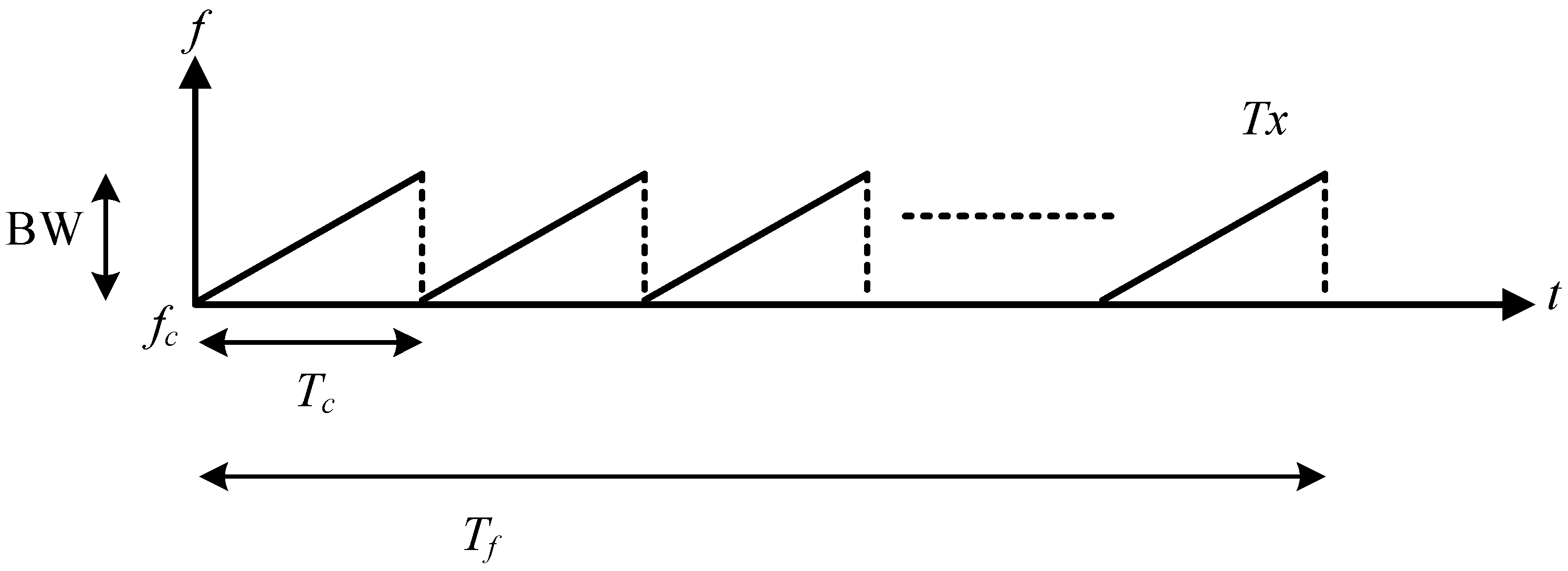
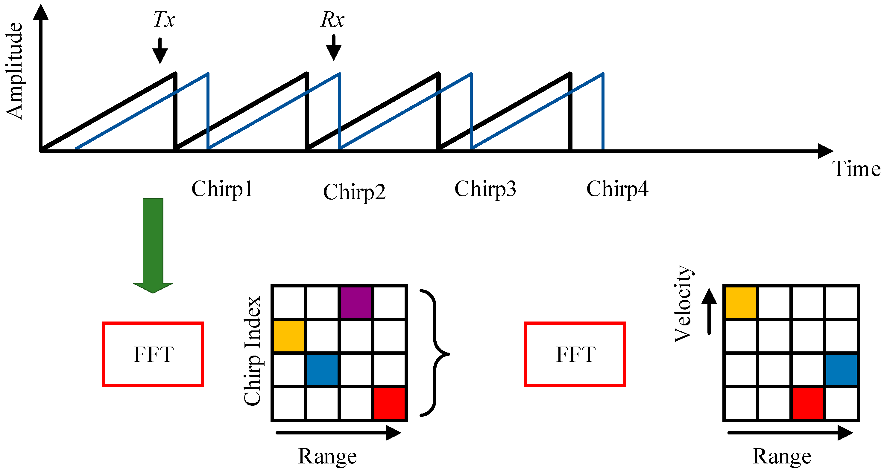
3.1. Automotive FMCW Radar
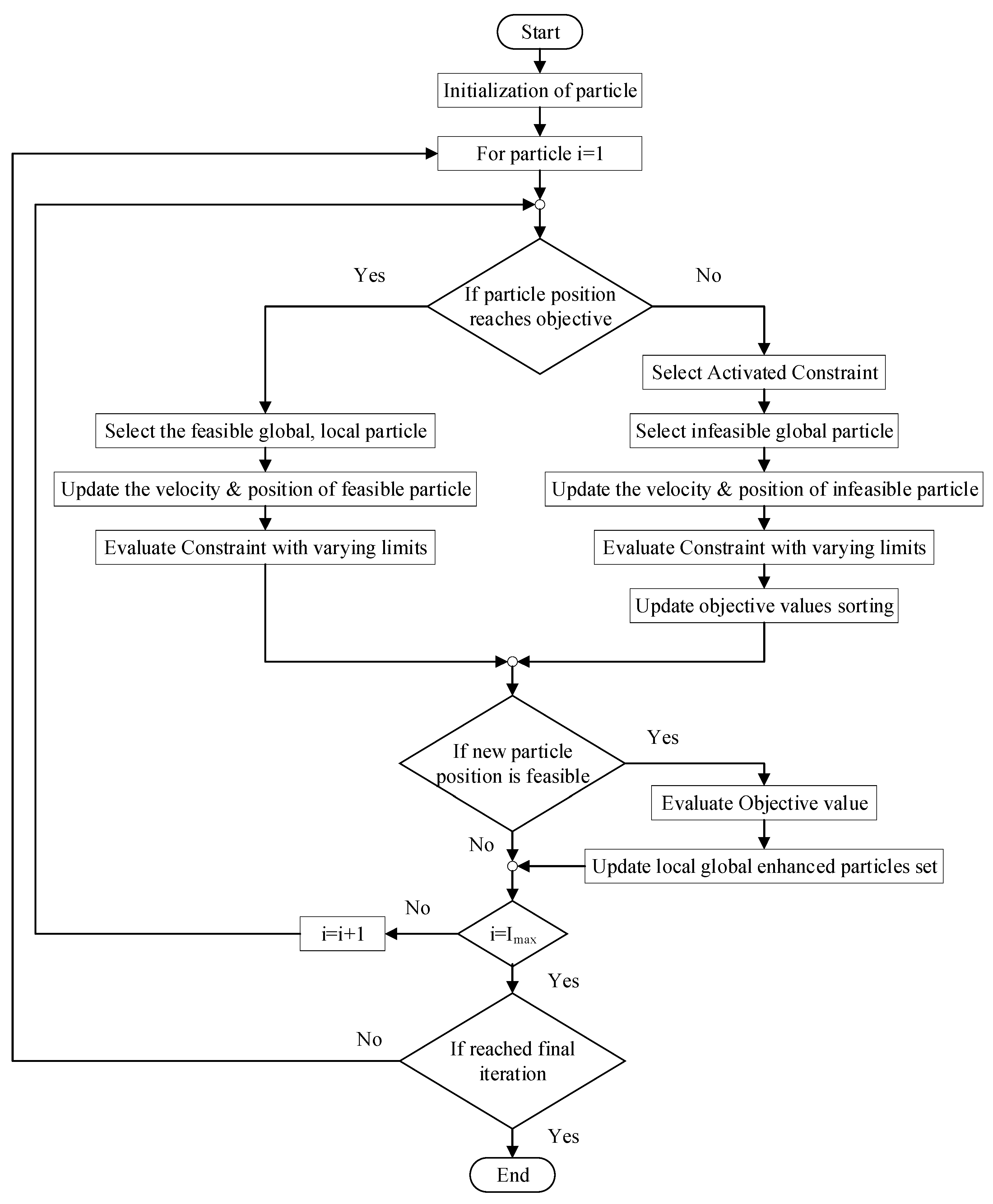
3.2. Proposed AOHDL Methodologies
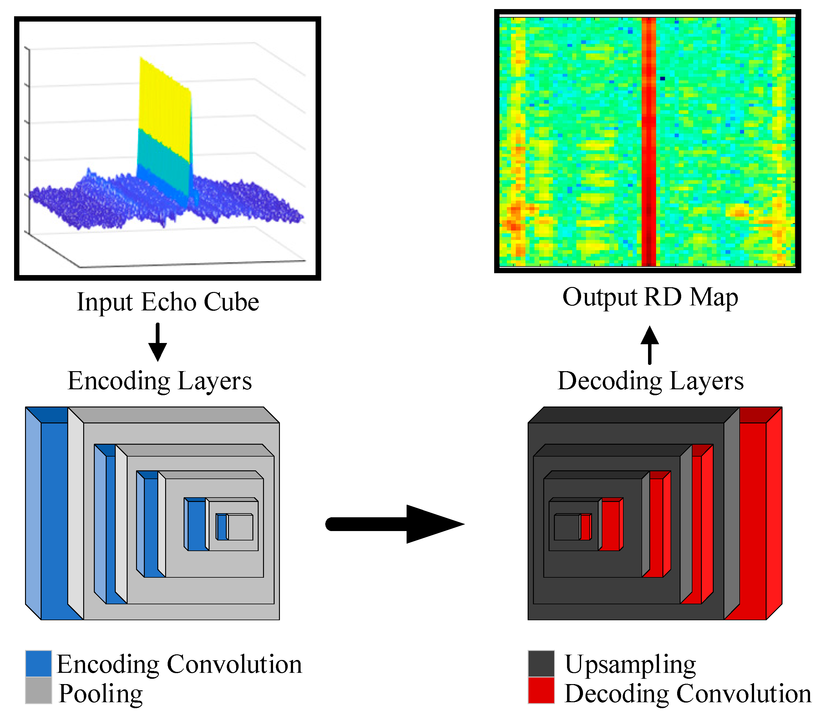
3.2.1. Coherent Echo Pulse Map
3.2.2. DAALnet-Based Feature Map Using Coherent Echo Pulse
3.2.3. FELLnet Design Methodologies
3.2.4. TDDLnet Formation
3.2.5. AHODnet Description
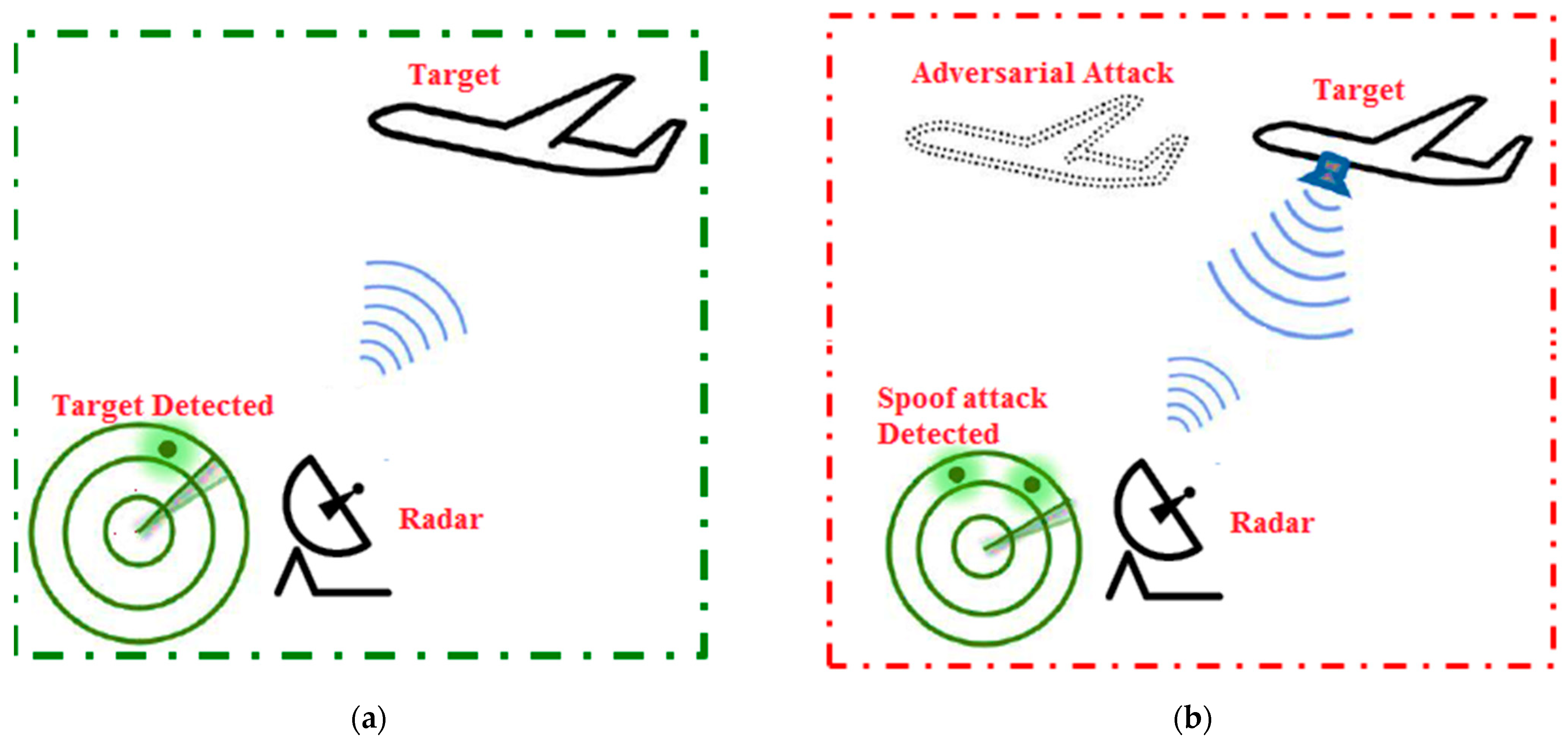
3.2.6. Adversarial Attack
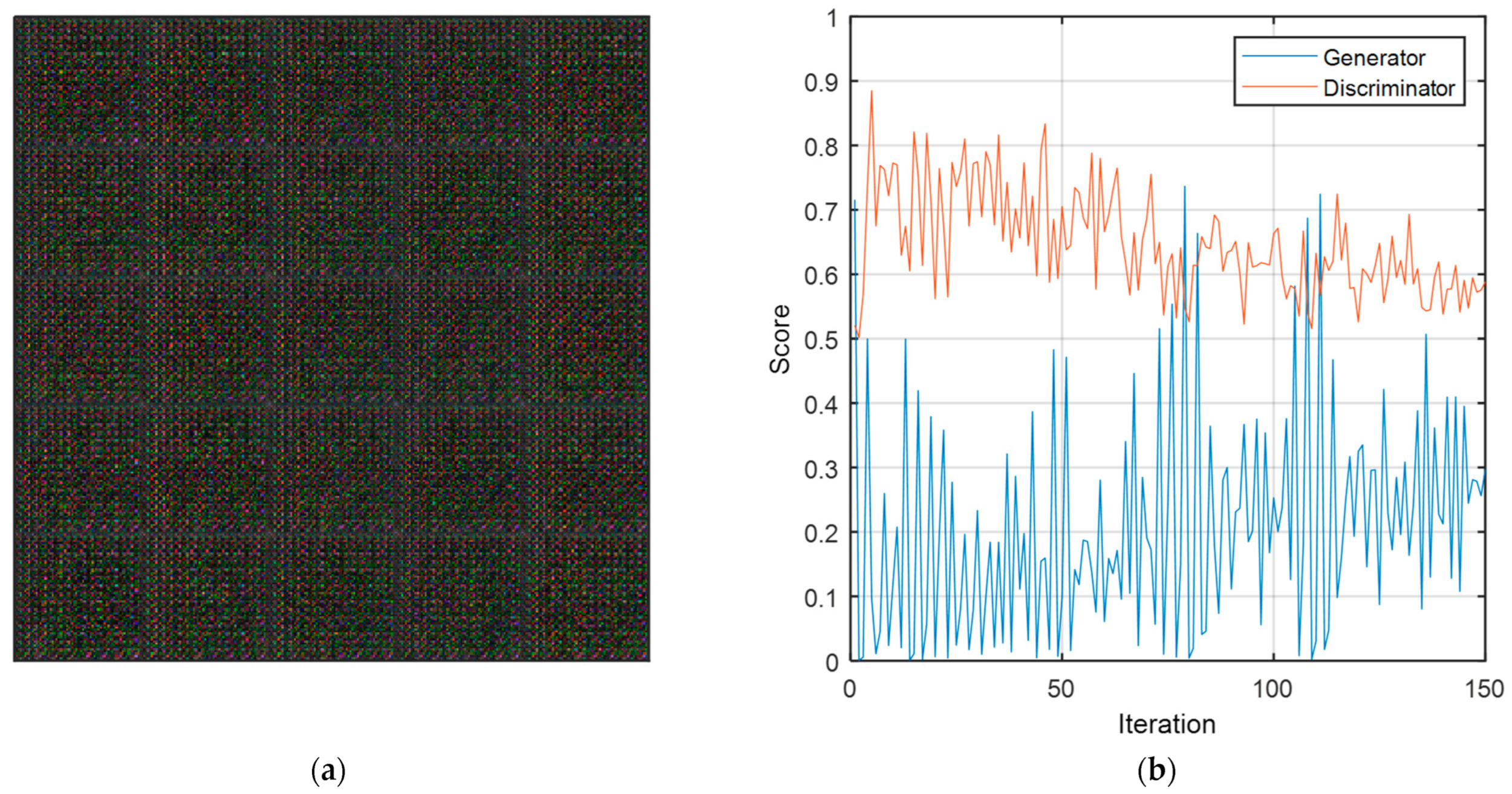
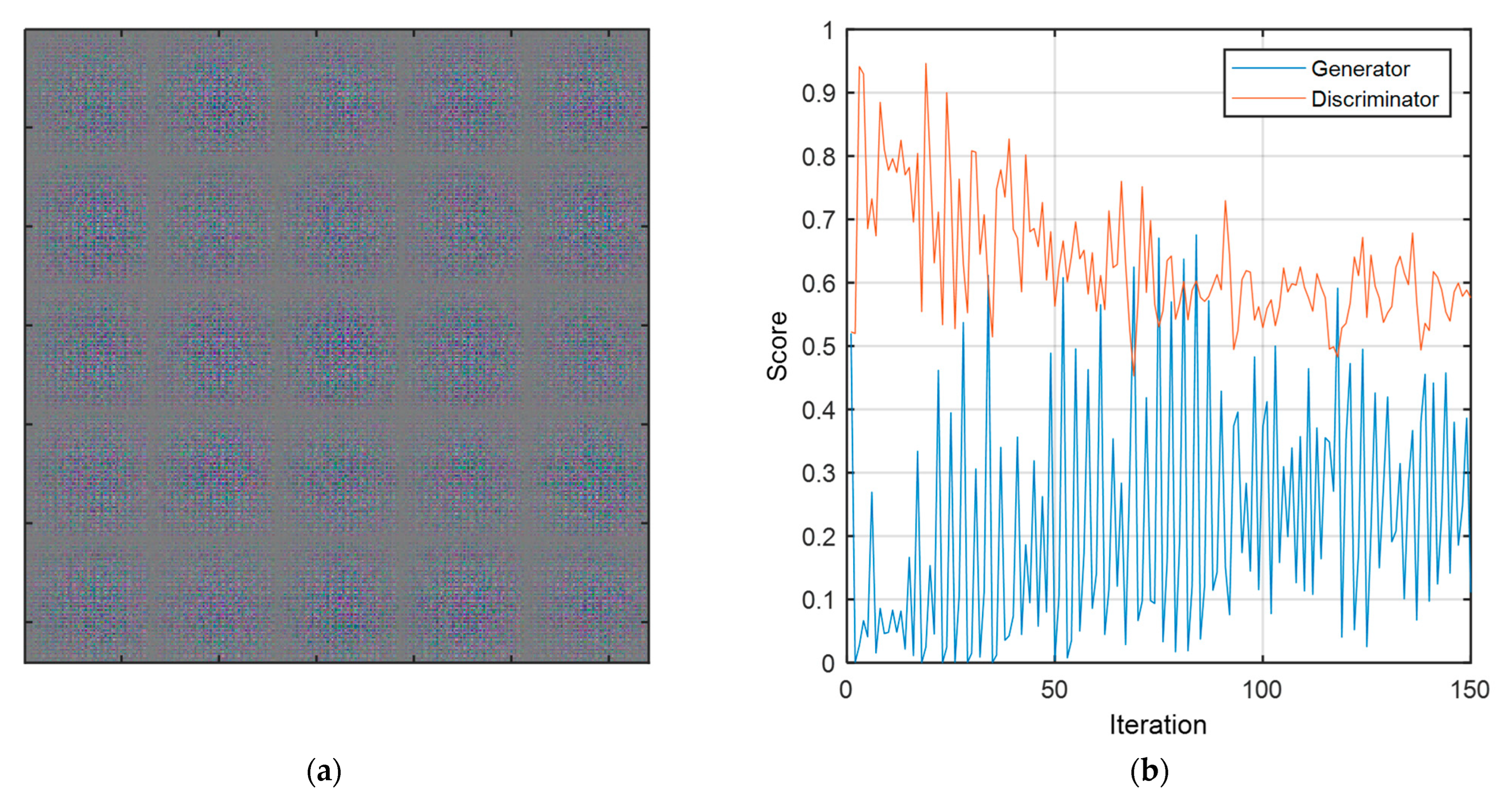
3.2.7. Adversarial Attack Networks
- The first idea is the robustness of the DLN model. This indicates that under this paradigm, the DLN model knows the least perturbation required to transform picture x into an adversarial attack image .
- Adversarial risk, or the gradient descent loss function of the DLN model, is the second property. By reducing errors concerning the input picture, the model aims to improve its prediction score during the DLN learning process. Therefore, the adversary tries to maximize the loss function in order to produce an adversarial picture. To accomplish this, locate the location within x’s neighborhood bounds that can trick the DLN model [29].
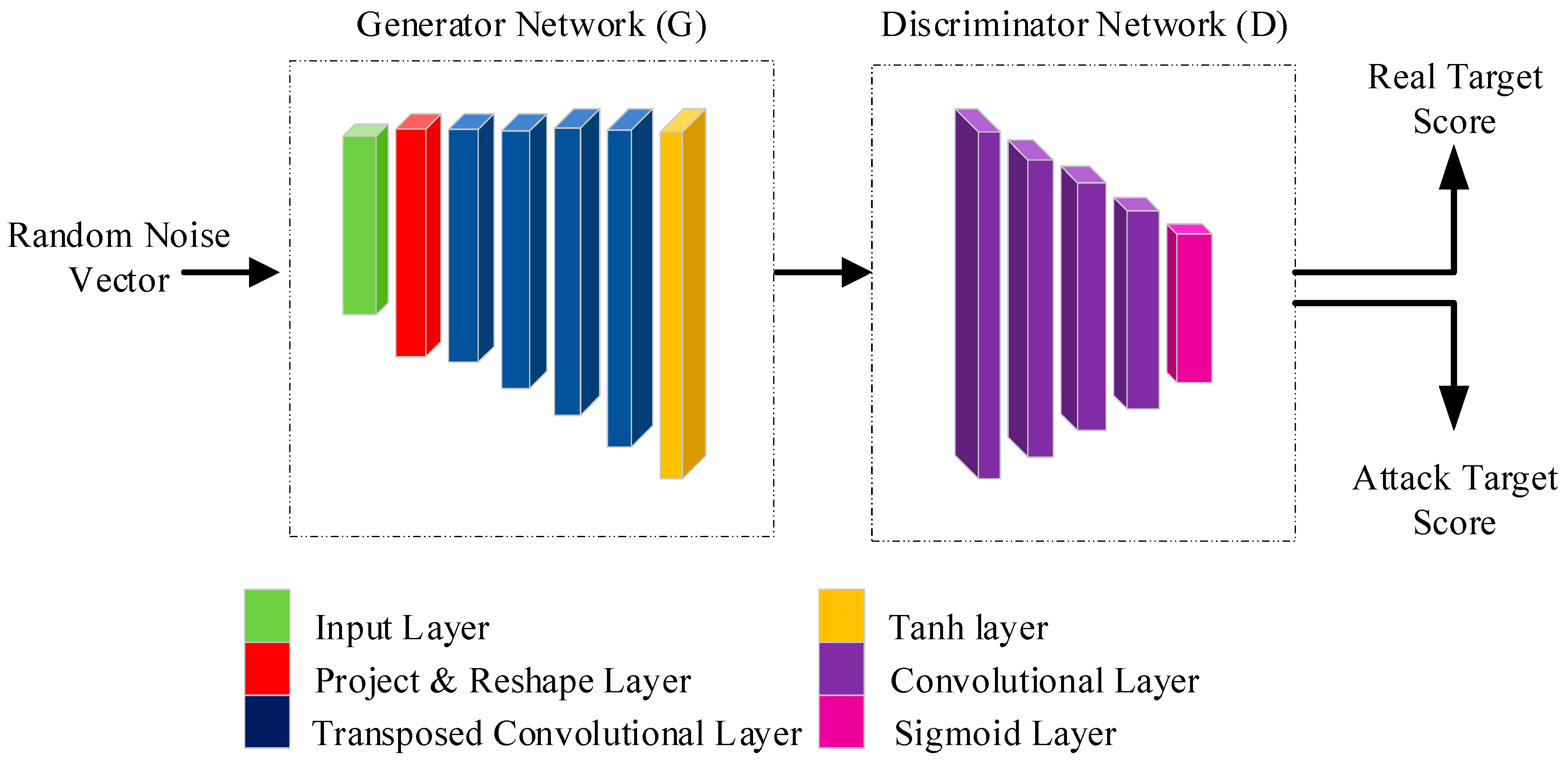
3.2.8. Radar Generative Adversarial Networks (GANs)
Adversarial Generator Network
Adversarial Discriminator Network
Cost Function of RGAN
4. Results and Discussion
4.1. Complexity Analysis of Adversarial Learning
4.2. Time Complexity of Computation in AOHDL
5. Conclusions
Author Contributions
Funding
Data Availability Statement
Conflicts of Interest
References
- Kaselimi, M.; Voulodimos, A.; Daskalopoulos, I.; Doulamis, N.; Doulamis, A. A vision transformer model for convolution-free multilabel classification of satellite imagery in deforestation monitoring. IEEE Trans. Neural Netw. Learn. Syst. 2022, 34, 3299–3307. [Google Scholar] [CrossRef]
- Park, K.-E.; Lee, J.-P.; Kim, Y. Deep learning-based indoor distance estimation scheme using FMCW radar. Information 2021, 12, 80. [Google Scholar] [CrossRef]
- Sun, S.; Petropulu, A.P.; Poor, H.V. MIMO radar for advanced driver-assistance systems and autonomous driving: Advantages and challenges. IEEE Signal Process. Mag. 2020, 37, 98–117. [Google Scholar] [CrossRef]
- Patole, S.M.; Torlak, M.; Wang, D.; Ali, M. Automotive radars: A review of signal processing techniques. IEEE Signal Process. Mag. 2017, 34, 22–35. [Google Scholar] [CrossRef]
- Lies, W.A.; Narula, L.; Iannucci, P.A.; Humphreys, T.E. Long range, low swap-C FMCW radar. IEEE J. Sel. Top. Signal Process. 2021, 15, 1030–1040. [Google Scholar] [CrossRef]
- Ordean, M.; Garcia, F.D. Millimeter-wave automotive radar spoofing. arXiv 2022, arXiv:2205.06567. [Google Scholar]
- Yuan, Y.; Wan, J.; Chen, B. Robust attack on deep learning based radar HRRP target recognition. In Proceedings of the 2019 Asia-Pacific Signal and Information Processing Association Annual Summit and Conference (APSIPA ASC), Lanzhou, China, 18–21 November 2019; pp. 704–707. [Google Scholar]
- Lin, W.; Shi, L.; Zhong, Y.; Huang, Y.; Ding, X. Improving Black-box Adversarial Attacks on HRRP-based Radar Automatic Target Recognition. In Proceedings of the 2021 CIE International Conference on Radar (Radar), Haikou, China, 15–19 December 2021; pp. 3206–3209. [Google Scholar]
- Geng, L.; Li, Y.; Dong, L.; Tan, Y.; Cheng, W. Efficiently Refining Beampattern in FDA-MIMO Radar via Alternating Manifold Optimization for Maximizing Signal-to-Interference-Noise Ratio. Remote Sens. 2024, 16, 1364. [Google Scholar] [CrossRef]
- Zafar, A.; Khan, A.; Younis, S. Classical Adversarial Attack on mm-Wave FMCW Radar. In Proceedings of the 2021 International Conference on Frontiers of Information Technology (FIT), Islamabad, Pakistan, 13–14 December 2021; pp. 281–286. [Google Scholar]
- Zheng, Y.; Su, J.; Zhang, S.; Tao, M.; Wang, L. Dehaze-AGGAN: Unpaired remote sensing image dehazing using enhanced attention-guide generative adversarial networks. IEEE Trans. Geosci. Remote Sens. 2022, 60, 1–13. [Google Scholar] [CrossRef]
- Valtl, J.; Issakov, V. Universal Adversarial Attacks on the Raw Data from a Frequency Modulated Continuous Wave Radar. IEEE Access 2022, 10, 114092–114102. [Google Scholar] [CrossRef]
- Tarchoun, B.; Alouani, I.; Khalifa, A.B.; Mahjoub, M.A. Adversarial attacks in a multi-view setting: An empirical study of the adversarial patches inter-view transferability. In Proceedings of the 2021 International Conference on Cyberworlds (CW), Caen, France, 28–30 September 2021; pp. 299–302. [Google Scholar]
- Guesmi, A.; Alouani, I. Adversarial attack on radar-based environment perception systems. arXiv 2022, arXiv:2211.01112. [Google Scholar]
- Hunt, D.; Angell, K.; Qi, Z.; Chen, T.; Pajic, M. MadRadar: A Black-Box Physical Layer Attack Framework on mmWave Automotive FMCW Radars. arXiv 2023, arXiv:2311.16024. [Google Scholar]
- Xu, Y.; Shi, L.; Lin, C.; Cai, S.; Lin, W.; Huang, Y.; Ding, X. A Contrastive-Based Adversarial Training Algorithm for HRRP Target Recognition. IEEE Geosci. Remote Sens. Lett. 2023, 20, 1–5. [Google Scholar] [CrossRef]
- Narasimhamurthy, R.; Khalaf, O.I. Deep Learning Network for Classifying Target of Same Shape using RCS Time Series. Air Traffic Manag. Control 2021, 9, 25. [Google Scholar]
- Cha, D.; Jeong, S.; Yoo, M.; Oh, J.; Han, D. Multi-input deep learning based FMCW radar signal classification. Electronics 2021, 10, 1144. [Google Scholar] [CrossRef]
- Klintberg, J.; McKelvey, T.; Dammert, P. A parametric approach to space-time adaptive processing in bistatic radar systems. IEEE Trans. Aerosp. Electron. Syst. 2021, 58, 1149–1160. [Google Scholar] [CrossRef]
- Mark, S.; Lokash, S.; Shashi, S. Trihedral Corner Reflector. Millimeter Wave Product. Available online: https://www.miwv.com/trihedral-reflectors-for-radar-applications/ (accessed on 14 June 2020).
- Mahafza, B.R. Radar Systems Analysis and Design Using MATLAB; Chapman and Hall/CRC: Boca Raton, FL, USA, 2005. [Google Scholar]
- Chen, H.-R. FMCW Radar Jamming Techniques and Analysis. Available online: https://core.ac.uk/download/pdf/36730041.pdf (accessed on 10 September 2013).
- Snihs, L. Evaluation of FMCW Radar Jamming Sensitivity. Available online: https://www.diva-portal.org/smash/get/diva2:1767179/FULLTEXT01.pdf (accessed on 14 June 2023).
- Xie, Y.; Jiang, R.; Guo, X.; Wang, Y.; Cheng, J.; Chen, Y. Universal Targeted Adversarial Attacks Against mmWave-based Human Activity Recognition. In Proceedings of the IEEE INFOCOM 2023-IEEE Conference on Computer Communications, New York, NY, USA, 17–20 May 2023; pp. 1–10. [Google Scholar]
- Carlini, N.; Wagner, D. Towards evaluating the robustness of neural networks. In Proceedings of the 2017 IEEE Symposium on Security and Privacy (SP), San Jose, CA, USA, 22–24 May 2017; pp. 39–57. [Google Scholar]
- Ozbulak, U.; Vandersmissen, B.; Jalalvand, A.; Couckuyt, I.; van Messem, A.; de Neve, W. Investigating the significance of adversarial attacks and their relation to interpretability for radar-based human activity recognition systems. Comput. Vis. Image Underst. 2021, 202, 103111. [Google Scholar] [CrossRef]
- Rahman, M.M.; Gurbuz, S.Z.; Amin, M.G. Physics-aware generative adversarial networks for radar-based human activity recognition. IEEE Trans. Aerosp. Electron. Syst. 2022, 59, 2994–3008. [Google Scholar] [CrossRef]
- Yue, Y.; Liu, H.; Meng, X.; Li, Y.; Du, Y. Generation of high-precision ground penetrating radar images using improved least square generative adversarial networks. Remote Sens. 2021, 13, 4590. [Google Scholar] [CrossRef]
- Chen, C.; Su, Y.; He, Z.; Liu, T.; Song, X. Clutter mitigation in holographic subsurface radar imaging using generative adversarial network with attentive subspace projection. IEEE Trans. Geosci. Remote Sens. 2022, 60, 1–14. [Google Scholar] [CrossRef]
- Chen, S.; Shangguan, W.; Taghia, J.; Kühnau, U.; Martin, R. Automotive radar interference mitigation based on a generative adversarial network. In Proceedings of the 2020 IEEE Asia-Pacific Microwave Conference (APMC), Hong Kong, China, 10–13 November 2020; pp. 728–730. [Google Scholar]
- Wang, S.; An, Q.; Li, S.; Zhao, G.; Sun, H. Wiring effects mitigation for through-wall human motion micro-doppler signatures using a generative adversarial network. IEEE Sens. J. 2021, 21, 10007–10016. [Google Scholar] [CrossRef]
- Pan, Z.; Wang, S.; Li, Y. Residual attention-aided U-Net GAN and multi-instance multilabel classifier for automatic waveform recognition of overlapping LPI radar signals. IEEE Trans. Aerosp. Electron. Syst. 2022, 58, 4377–4395. [Google Scholar] [CrossRef]
- Wang, H.; Li, K.; Lu, X.; Zhang, Q.; Luo, Y.; Kang, L. ISAR Resolution Enhancement Method Exploiting Generative Adversarial Network. Remote Sens. 2022, 14, 1291. [Google Scholar] [CrossRef]
- Wang, C.; Wang, P.; Wang, P.; Xue, B.; Wang, D. Using conditional generative adversarial 3-D convolutional neural network for precise radar extrapolation. IEEE J. Sel. Top. Appl. Earth Obs. Remote Sens. 2021, 14, 5735–5749. [Google Scholar] [CrossRef]
- Che, J.; Wang, L.; Wang, C.; Zhou, F. A Novel Adversarial Learning Framework for Passive Bistatic Radar Signal Enhancement. Electronics 2023, 12, 3072. [Google Scholar] [CrossRef]
- Zhu, Y.; Miao, C.; Xue, H.; Li, Z.; Yu, Y.; Xu, W.; Su, L.; Qiao, C. TileMask: A Passive-Reflection-based Attack against mmWave Radar Object Detection in Autonomous Driving. In Proceedings of the 2023 ACM SIGSAC Conference on Computer and Communications Security, New York, NY, USA, 26–30 November 2023; pp. 1317–1331. [Google Scholar]
- Almutairi, S.; Barnawi, A. Securing DNN for smart vehicles: An overview of adversarial attacks, defenses, and frameworks. J. Eng. Appl. Sci. 2023, 70, 16. [Google Scholar] [CrossRef]
- Graff, A.M.; Humphreys, T.E. Signal Identification and Entrainment for Practical FMCW Radar Spoofing Attacks. In Proceedings of the 2023 IEEE 97th Vehicular Technology Conference (VTC2023-Spring), Florence, Italy, 20–23 June 2023; pp. 1–7. [Google Scholar]
- Xue, W.; Wang, R.; Liu, L.; Wu, D. Accurate multi-target vital signs detection method for FMCW radar. Measurement 2023, 223, 113715. [Google Scholar] [CrossRef]
- Chen, S.; Taghia, J.; Fei, T.; Kühnau, U.; Pohl, N.; Martin, R. A DNN autoencoder for automotive radar interference mitigation. In Proceedings of the ICASSP 2021—2021 IEEE International Conference on Acoustics, Speech and Signal Processing (ICASSP), Toronto, ON, Canada, 6–11 June 2021; pp. 4065–4069. [Google Scholar]
- Liang, S.; Chen, R.; Duan, G.; Du, J. Deep learning-based lightweight radar target detection method. J. Real-Time Image Process. 2023, 20, 61. [Google Scholar] [CrossRef]
- Wang, J.; Li, S. SALA-LSTM: A novel high-precision maritime radar target detection method based on deep learning. Sci. Rep. 2023, 13, 12125. [Google Scholar] [CrossRef]
- Ishaq, M.; Kwon, S. A CNN-Assisted deep echo state network using multiple Time-Scale dynamic learning reservoirs for generating Short-Term solar energy forecasting. Sustain. Energy Technol. Assess. 2022, 52, 102275. [Google Scholar]
- Mikolov, T.; Karafiát, M.; Burget, L.; Cernocký, J.; Khudanpur, S. Recurrent neural network based language model. In Proceedings of the Interspeech 2010, Makuhari, Japan, 26–30 September 2010; Volume 2, pp. 1045–1048. [Google Scholar]
- Wan, R.; Song, Y.; Mu, T.; Wang, Z. Moving target detection using the 2D-FFT algorithm for automotive FMCW radars. In Proceedings of the 2019 International Conference on Communications, Information System and Computer Engineering (CISCE), Haikou, China, 5–7 July 2019; pp. 239–243. [Google Scholar]
- Lee, S.; Lee, B.-H.; Lee, J.-E.; Kim, S.-C. Statistical characteristic-based road structure recognition in automotive FMCW radar systems. IEEE Trans. Intell. Transp. Syst. 2018, 20, 2418–2429. [Google Scholar] [CrossRef]
- Tsipras, D.; Santurkar, S.; Engstrom, L.; Turner, A.; Madry, A. Robustness may be at odds with accuracy. arXiv 2018, arXiv:1805.12152. [Google Scholar]
- Kandel, I.; Castelli, M. The effect of batch size on the generalizability of the convolutional neural networks on a histopathology dataset. ICT Express 2020, 6, 312–315. [Google Scholar] [CrossRef]


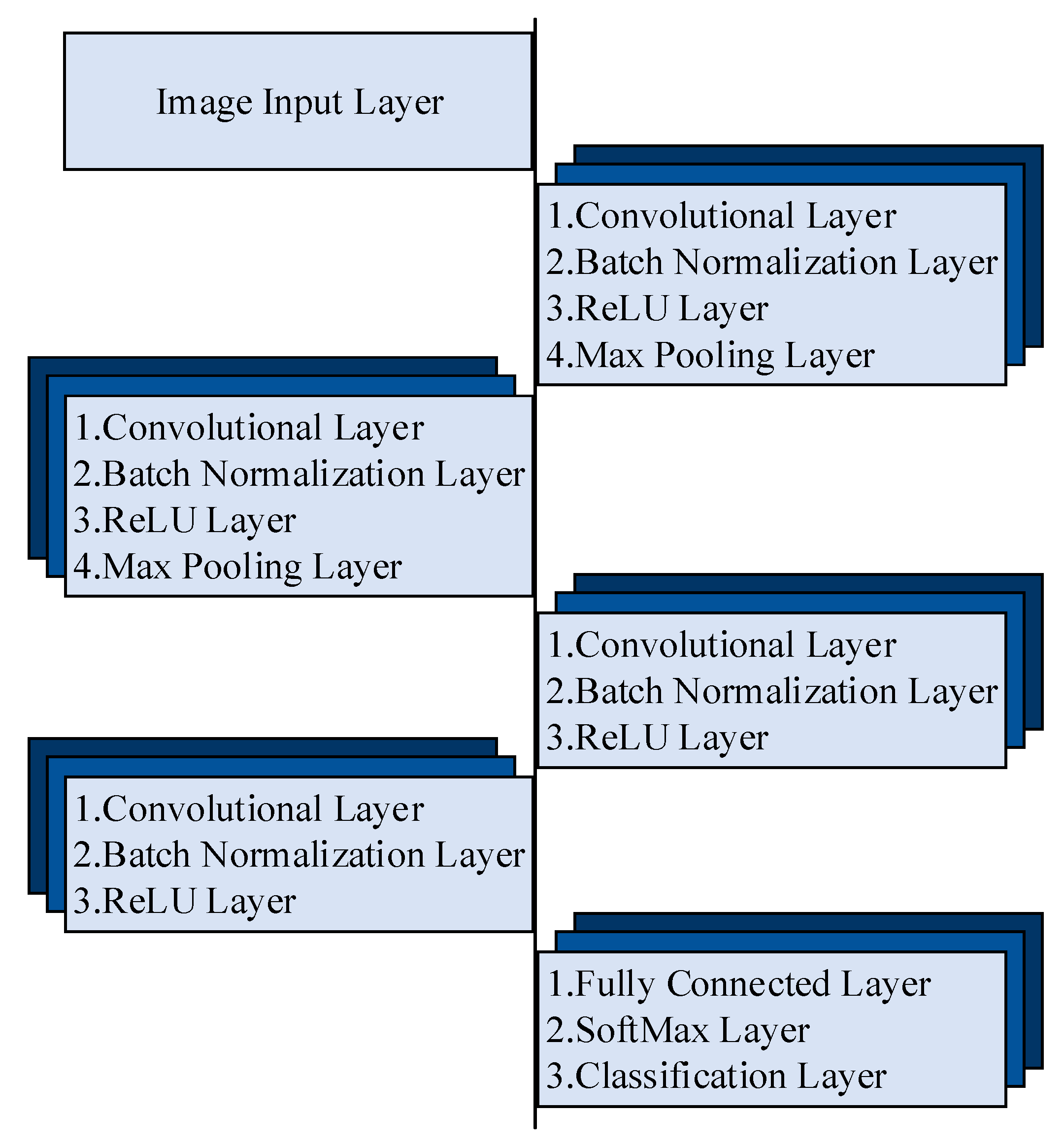
| Layer Type | Activations | Learnables | Layer Type | Activations | Learnables | |
|---|---|---|---|---|---|---|
| Image Input | 224 × 224 × 3 | - | Addition | 28 × 28 × 128 | - | |
| Convolution | 112 × 112 × 64 | Weights—7 × 7 × 3 × 64 | ReLU | 28 × 28 × 128 | - | |
| Bias—1 × 1 × 64 | ID Block 3 | 28 × 28 × 128 | Weights—3 × 3 × 128 × 128 | |||
| Batch Normalization | 112 × 112 × 64 | Offset—1 × 1 × 64 | Bias—1 × 1 × 128 | |||
| Scale—1 × 1 × 64 | DS Block 2 | 14 × 14 × 256 | Weights—1 × 1 × 128 × 256 | |||
| ReLU | 112 × 112 × 64 | - | Bias—1 × 1 × 256 | |||
| Max Pooling | 56 × 56 × 64 | - | Addition | 14 × 14 × 256 | - | |
| ID Block 1 | Convolution | 56 × 56 × 64 | Weights—3 × 3 × 64 × 64 | ReLU | 14 × 14 × 256 | - |
| Bias—1 × 1 × 64 | ID Block 4 | 14 × 14 × 256 | Weights—3 × 3 × 256 × 256 | |||
| Batch Normalization | 56 × 56 × 64 | Offset—1 × 1 × 16 | Bias—1 × 1 × 256 | |||
| Scale—1 × 1 × 16 | DS Block 3 | 7 × 7 × 512 | Weights—1 × 1 × 256 × 512 | |||
| ReLU | 56 × 56 × 64 | - | Bias—1 × 1 × 512 | |||
| Convolution | 56 × 56 × 64 | Weights—3 × 3 × 64 × 64 | Addition | 7 × 7 × 512 | - | |
| Bias—1 × 1 × 64 | ReLU | 7 × 7 × 512 | - | |||
| Batch Normalization | 56 × 56 × 64 | Offset—1 × 1 × 64 | ID Block 5 | 7 × 7 × 512 | Weights—3 × 3 × 512 × 512 | |
| Scale—1 × 1 × 64 | Bias—1 × 1 × 512 | |||||
| Addition | 56 × 56 × 64 | - | Addition | 7 × 7 × 512 | - | |
| ReLU | 56 × 56 × 64 | - | ReLU | 7 × 7 × 512 | - | |
| ID Block 2 | 56 × 56 × 64 | Weights—3 × 3 × 64 × 64 | —Average Pooling | 1 × 1 × 512 | - | |
| Bias—1 × 1 × 64 | Fully Connected | 1 × 1 × 3 | Weights—3 × 512 | |||
| DS Block 1 | Convolution | 28 × 28 × 128 | Weights—3 × 3 × 64 × 128 | Bias—3 × 1 | ||
| Bias—1 × 1 × 128 | Softmax | 1 × 1 × 3 | - | |||
| Batch Normalization | 28 × 28 × 128 | Offset—1 × 1 × 128 | Classification | - | - | |
| Scale—1 × 1 × 128 | ||||||
| ReLU | 28 × 28 × 128 | - | ||||
| Convolution | 28 × 28 × 128 | Weights—3 × 3 × 128 × 128 | ||||
| Bias—1 × 1 × 128 | ||||||
| Batch Normalization | 28 × 28 × 128 | Offset—1 × 1 × 128 | ||||
| Scale—1 × 1 × 128 | ||||||
| Convolution | 28 × 28 × 128 | Weights—1 × 1 × 64 × 128 | ||||
| Bias—1 × 1 × 128 | ||||||
| Batch Normalization | 28 × 28 × 128 | Offset—1 × 1 × 128 | ||||
| Scale—1 × 1 × 128 | ||||||
| Layer Type | Activations | Learnables | Layer Type | Activations | Learnables | ||
|---|---|---|---|---|---|---|---|
| Image Input | 32 × 32 × 1 | - | Decoding Layers | Transposed Convolution | 2 × 2 × 2 | Weights—4 × 4 × 2 × 2 | |
| Encoding Layers | Convolution | 32 × 32 × 32 | Weights—3 × 3 × 1 × 32 | Bias—1 × 1 × 2 | |||
| Bias—1 × 1 × 32 | ReLU | 2 × 2 × 2 | - | ||||
| ReLU | 32 × 32 × 32 | - | Transposed Convolution | 16 × 16 × 16 | Weights—3 × 3 × 32 × 16 | ||
| Max Pooling | 16 × 16 × 32 | - | Bias—1 × 1 × 16 | ||||
| Convolution | 16 × 16 × 16 | Weights—3 × 3 × 32 × 16 | ReLU | 16 × 16 × 16 | - | ||
| Bias—1 × 1 × 16 | Transposed Convolution | 8 × 8 × 8 | Weights—3 × 3 × 16 × 8 | ||||
| ReLU | 16 × 16 × 16 | - | Bias—1 × 1 × 8 | ||||
| Max Pooling | 8 × 8 × 16 | - | ReLU | 8 × 8 × 8 | - | ||
| Convolution | 8 × 8 × 8 | Weights—3 × 3 × 16 × 8 | Transposed Convolution | 4 × 4 × 4 | Weights—3 × 3 × 8 × 4 | ||
| Bias—1 × 1 × 8 | Bias—1 × 1 × 4 | ||||||
| ReLU | 8 × 8 × 8 | - | ReLU | 4 × 4 × 4 | - | ||
| Max Pooling | 4 × 4 × 8 | - | Transposed Convolution | 2 × 2 × 2 | Weights—3 × 3 × 4 × 2 | ||
| Convolution | 4 × 4 × 4 | Weights—3 × 3 × 8 × 4 | Bias—1 × 1 × 2 | ||||
| Bias—1 × 1 × 4 | ReLU | 2 × 2 × 2 | - | ||||
| ReLU | 4 × 4 × 4 | - | Regression Output | 32 × 32 × 1 | - | ||
| Max Pooling | 2 × 2 × 4 | - | |||||
| Convolution | 2 × 2 × 2 | Weights—3 × 3 × 4 × 2 | |||||
| Bias—1 × 1 × 2 | |||||||
| ReLU | 2 × 2 × 2 | - | |||||
| Max Pooling | 1 × 1 × 2 | - |
| Layer Type | Activations | Learnables | Layer Type | Activations | Learnables | |
|---|---|---|---|---|---|---|
| Image Input | 32 × 32 × 3 | - | CCUnit(2, 1) | 16 × 16 × 32 | Weights—3 × 3 × 16 × 32 | |
| Convolution | 32 × 32 × 16 | Weights—3 × 3 × 3 × 16 | Bias—1 × 1 × 32 | |||
| Bias—1 × 1 × 16 | Addition | 16 × 16 × 32 | - | |||
| Batch Normalization | 32 × 32 × 16 | Offset—1 × 1 × 64 | ReLU | 16 × 16 × 32 | - | |
| Scale—1 × 1 × 64 | CCUnit(2, 2) | 16 × 16 × 32 | Weights—3 × 3 × 16 × 32 | |||
| ReLU | 32 × 32 × 16 | - | Bias—1 × 1 × 32 | |||
| Combined Convolutional Unit(1,1) | Convolution | 32 × 32 × 16 | Weights—3 × 3 × 16 × 16 Bias—1 × 1 × 16 | Addition | 16 × 16 × 32 | - |
| Batch Normalization | 32 × 32 × 16 | Offset –1 × 1 × 16 | ReLU | 16 × 16 × 32 | - | |
| Scale—1 × 1 × 16 | CCUnit(3, 1) | 8 × 8 × 64 | Weights—3 × 3 × 32 × 64 | |||
| ReLU | 32 × 32 × 16 | - | Bias—1 × 1 × 64 | |||
| Convolution | 32 × 32 × 16 | Weights—3 × 3 × 16 × 16 | Addition | 8 × 8 × 64 | - | |
| Bias—1 × 1 × 16 | ReLU | 8 × 8 × 64 | - | |||
| Batch Normalization | 32 × 32 × 16 | Offset –1 × 1 × 16 | CCUnit(3, 2) | 8 × 8 × 64 | Weights—3 × 3 × 64 × 64 | |
| Scale—1 × 1 × 16 | Bias—1 × 1 × 64 | |||||
| Addition | 32 × 32 × 16 | - | Addition | 8 × 8 × 64 | - | |
| ReLU | 32 × 32 × 16 | - | ReLU | 8 × 8 × 64 | - | |
| CCUnit(1, 2) | 32 × 32 × 16 | Weights—3 × 3 × 16 × 16 | Average Pooling | 5 × 5 × 64 | - | |
| Bias—1 × 1 × 16 | Fully Connected | 1 × 1 × 150 | Weights—150 × 1600 | |||
| Addition | 32 × 32 × 16 | - | Bias—150 × 1 | |||
| ReLU | 32 × 32 × 16 | - | Softmax | 1 × 1 × 150 | - |
| Adversarial Attack Types | Description | Function |
|---|---|---|
| Untargeted Attack | Sample-specific attack design. Aim to confuse prediction state from the original duplicate. | A(i + ψ) ≠ o |
| A is the deep learning model, i is the original sample, is generated adversarial perturbation, and o is the original prediction. | ||
| Targeted Attack | Sample-specific attack design. Aim to make the system predict the desired category. | A(i + ψ) = m |
| m is a predefined category | ||
| Universal Attack | Well-designed general perturbation. Inserting perturbation into unseen samples. | A(iu + ψ) = m |
| Iu is a different sample from the same class | ||
| Black-Box Attack | Attacking an unknown ML model. Perturbation of one model applied to another model. | Ab (ib) = A(ib) |
| Ab is another model than A and ib is adversarial samples produced using model A | ||
| White-Box Attack | Attacking a Known ML model. Perturbation is added to increase the loss. | A(ib+ψ*sign(Δ(ib)) = A(ib) |
| Δib is the magnitude of the gradient of the sample |
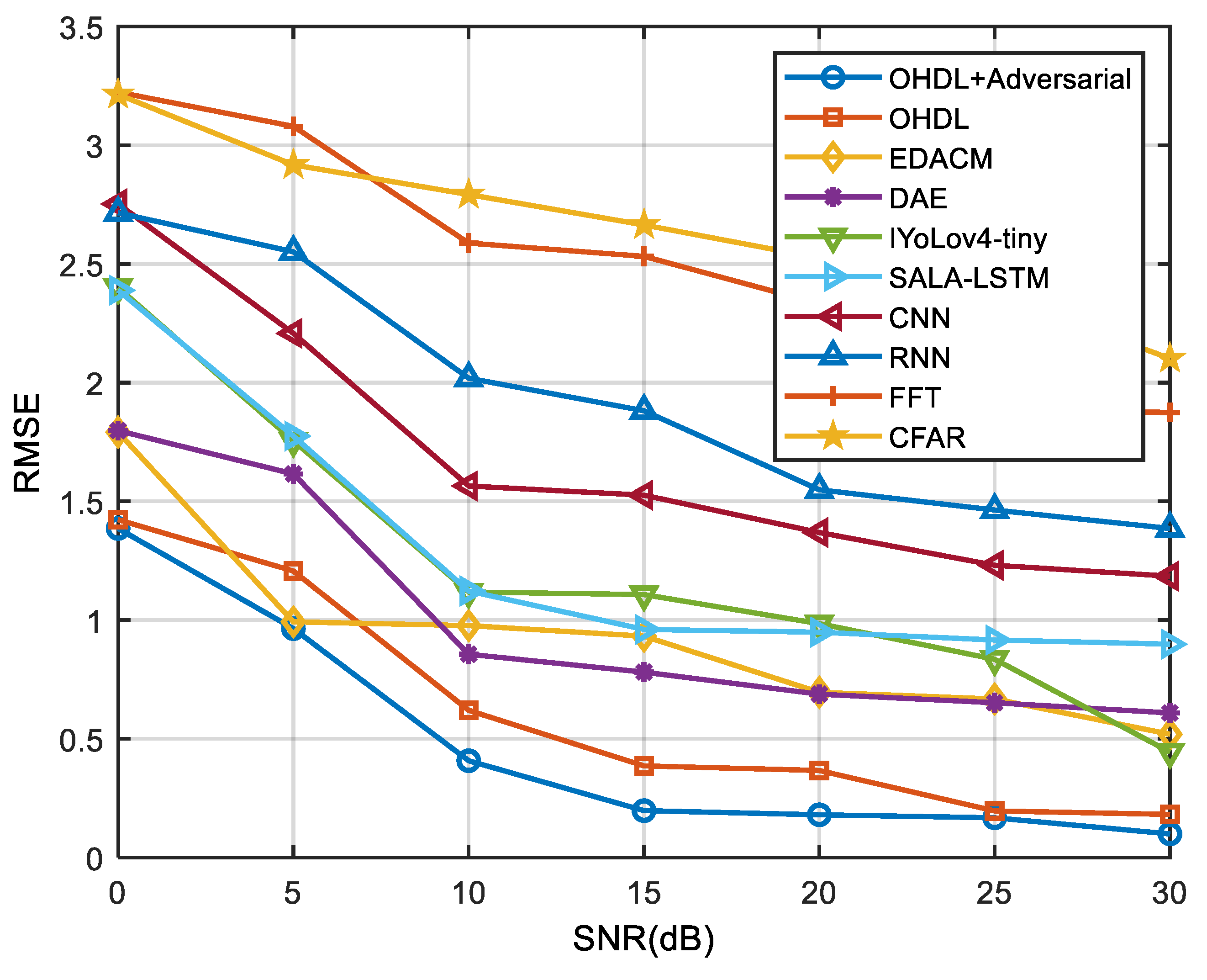
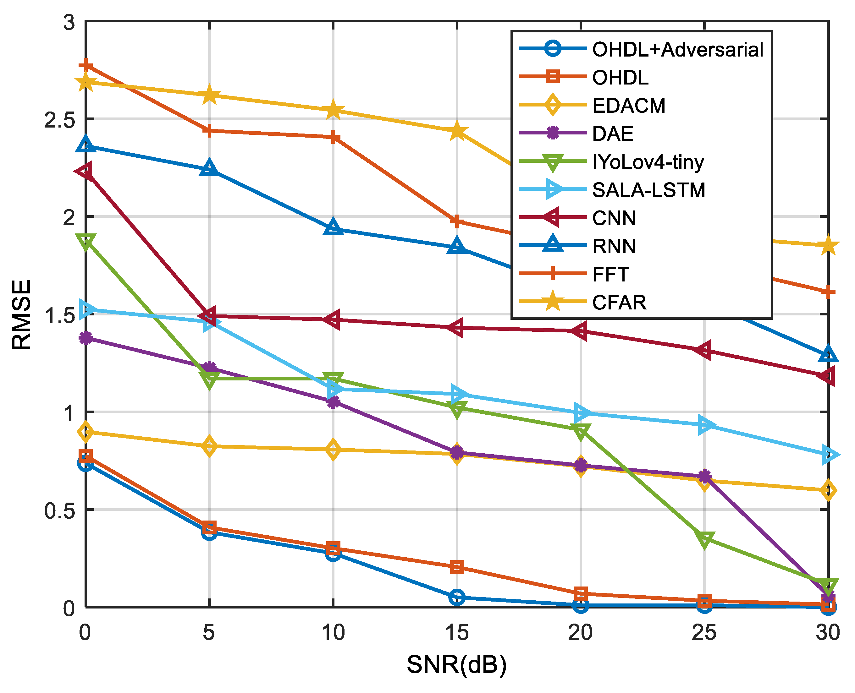
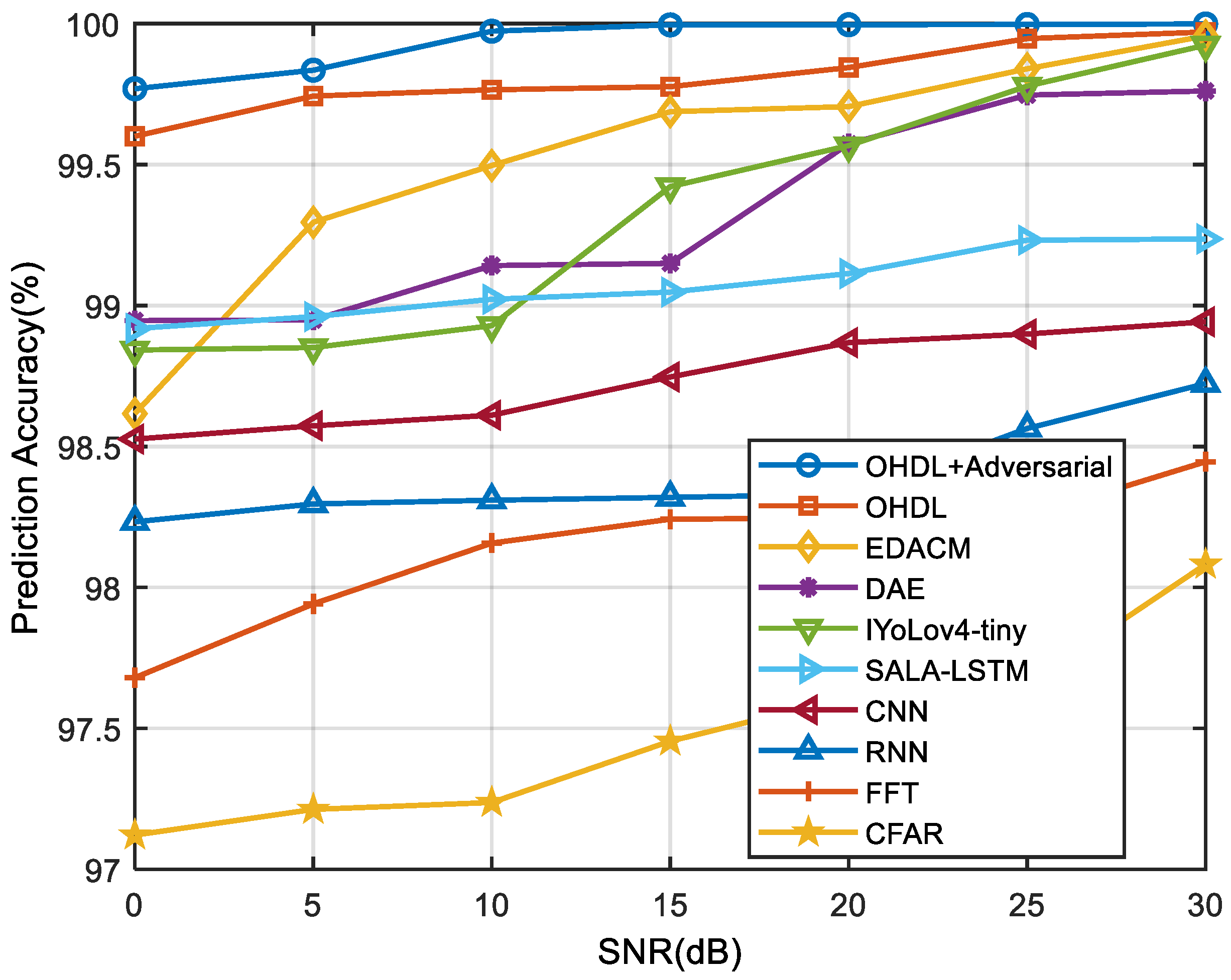
| Method | Proposed AOHDL | Proposed OHDL | EDACM | DAE | IYoLov4-tiny | SALA-LSTM | CNN | RNN | FFT | CFAR |
|---|---|---|---|---|---|---|---|---|---|---|
| SNR (dB) | ||||||||||
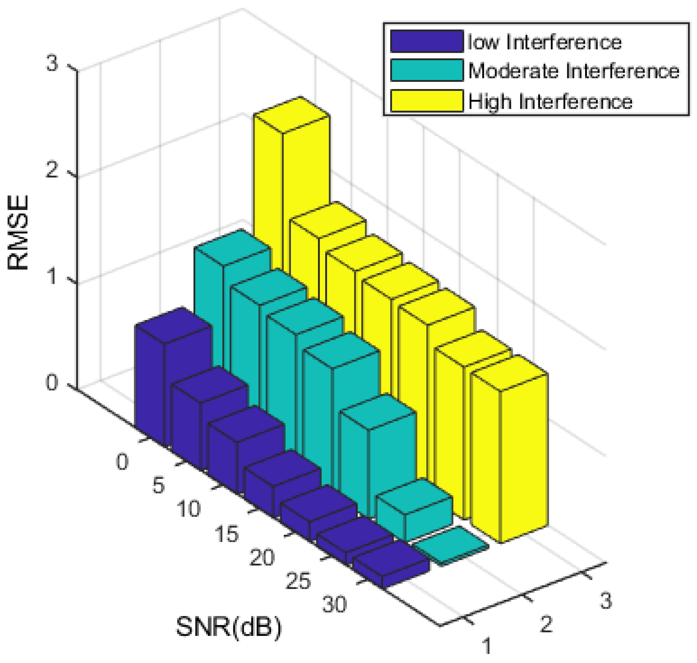
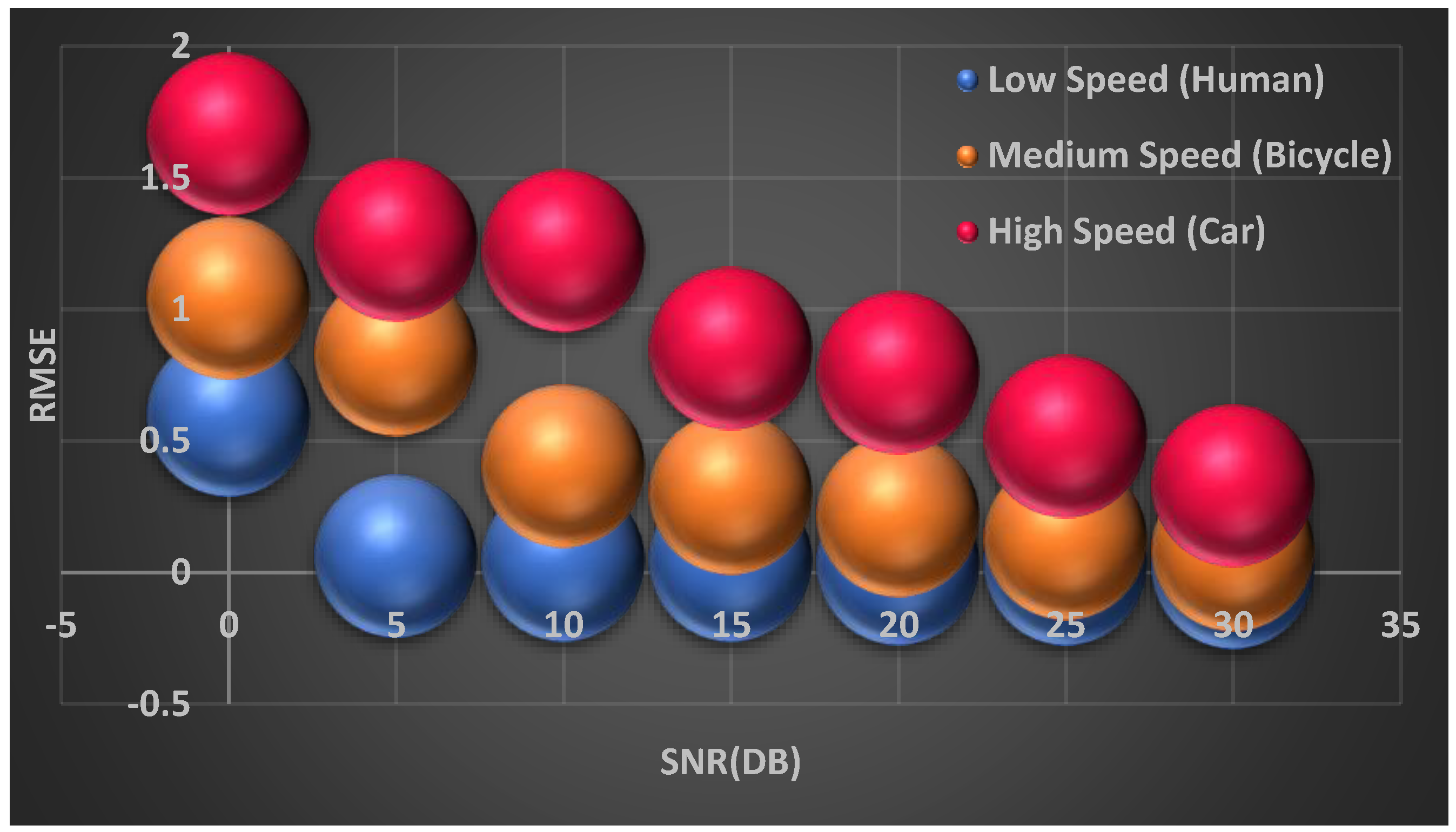
| 0 | 1.3858 | 1.4230 | 1.7912 | 1.7979 | 2.4006 | 2.3890 | 2.7525 | 2.7151 | 3.2233 | 3.2134 |
| 5 | 0.9641 | 1.2064 | 0.9926 | 1.6154 | 1.7551 | 1.7749 | 2.2075 | 2.5508 | 3.0792 | 2.9172 |
| 10 | 0.4077 | 0.6199 | 0.9768 | 0.8561 | 1.1182 | 1.1223 | 1.5647 | 2.0185 | 2.5877 | 2.7920 |
| 15 | 0.1974 | 0.3859 | 0.9323 | 0.7807 | 1.1074 | 0.9606 | 1.5259 | 1.8816 | 2.5317 | 2.6641 |
| 20 | 0.1800 | 0.3666 | 0.6957 | 0.6879 | 0.9850 | 0.9490 | 1.3687 | 1.5487 | 2.3325 | 2.5249 |
| 25 | 0.1673 | 0.1963 | 0.6677 | 0.6518 | 0.8349 | 0.9161 | 1.2309 | 1.4634 | 1.8885 | 2.3750 |
| 30 | 0.0994 | 0.1816 | 0.5191 | 0.6090 | 0.4445 | 0.8986 | 1.1848 | 1.3858 | 1.8745 | 2.1016 |
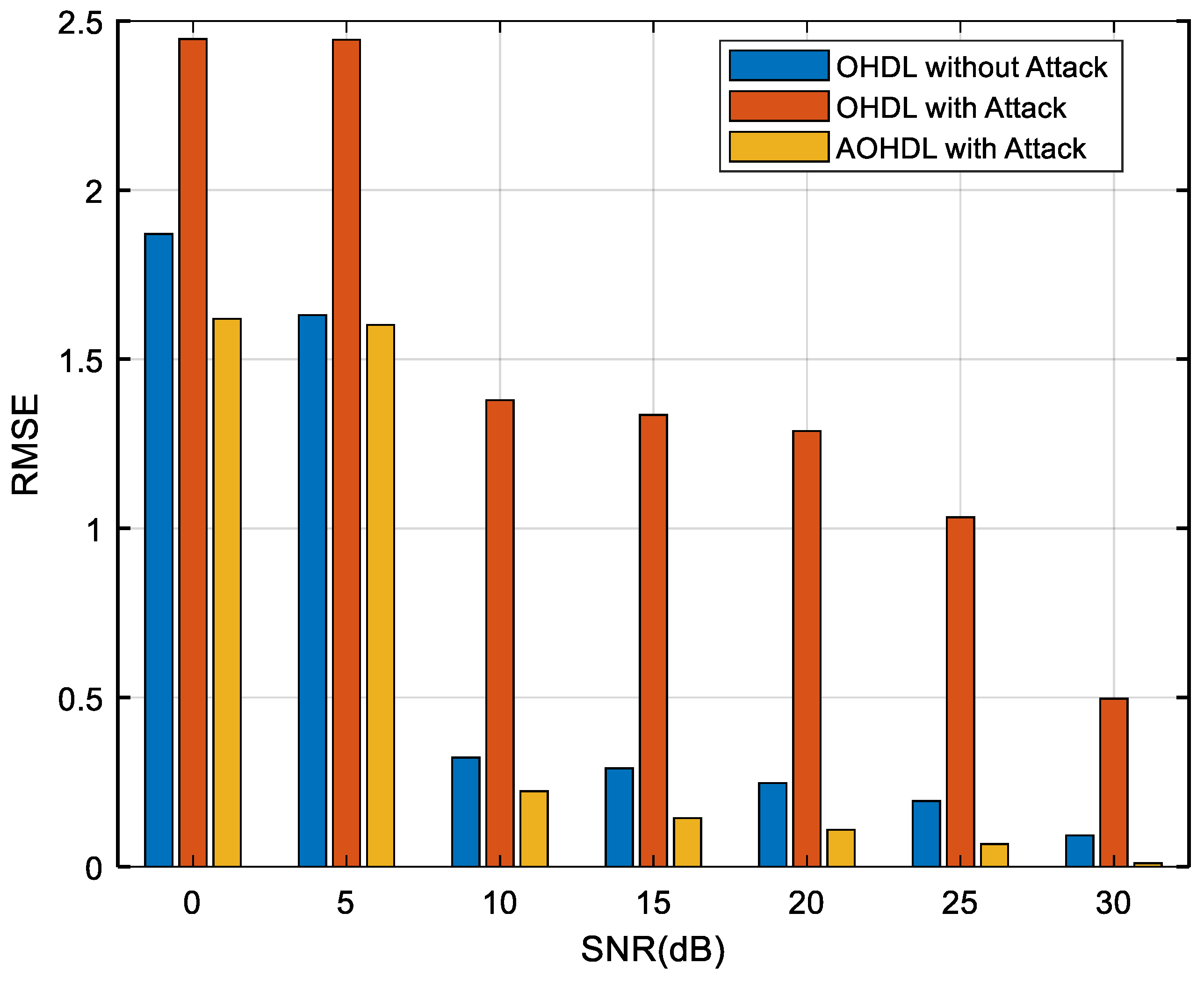
| Method | Proposed AOHDL | Proposed OHDL | EDACM | DAE | IYoLov4-tiny | SALA-LSTM | CNN | RNN | FFT | CFAR |
|---|---|---|---|---|---|---|---|---|---|---|
| SNR (dB) | ||||||||||
| 0 | 0.7364 | 0.7738 | 0.8977 | 1.3787 | 1.8796 | 1.5243 | 2.2306 | 2.3600 | 2.7736 | 2.6874 |
| 5 | 0.3837 | 0.4085 | 0.8238 | 1.2244 | 1.1700 | 1.4605 | 1.4903 | 2.2395 | 2.4385 | 2.6203 |
| 10 | 0.2759 | 0.3018 | 0.8069 | 1.0524 | 1.1696 | 1.1170 | 1.4716 | 1.9356 | 2.4062 | 2.5430 |
| 15 | 0.0502 | 0.2057 | 0.7839 | 0.7919 | 1.0218 | 1.0909 | 1.4305 | 1.8407 | 1.9735 | 2.4357 |
| 20 | 0.0104 | 0.0695 | 0.7217 | 0.7255 | 0.9082 | 0.9946 | 1.4134 | 1.6086 | 1.8396 | 2.0496 |
| 25 | 0.0104 | 0.0332 | 0.6484 | 0.6692 | 0.3538 | 0.9330 | 1.3150 | 1.5648 | 1.7609 | 1.9006 |
| 30 | 0.0000 | 0.0139 | 0.5982 | 0.0599 | 0.1157 | 0.7809 | 1.1825 | 1.2869 | 1.6136 | 1.8503 |
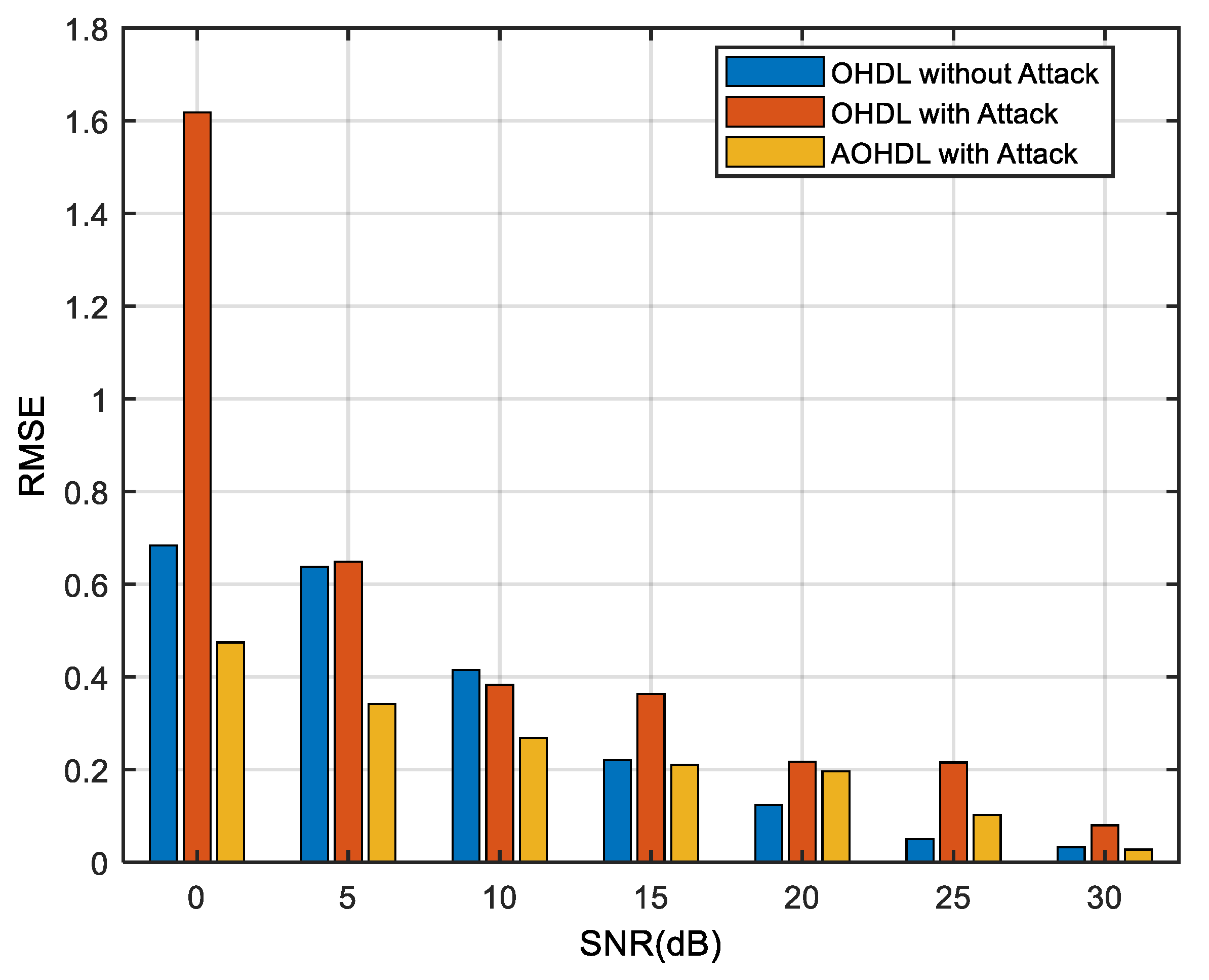
| KPI | Implementation Methods | ||
|---|---|---|---|
| OHDL without Attack | OHDL with Attack | AOHDL with Attack | |
| Accuracy (%) | 99.40 | 97.52 | 99.10 |
| Precision (%) | 99.39 | 97.49 | 99.11 |
| Recall (%) | 99.41 | 97.72 | 99.10 |
| FPR | 0.30 | 0.87 | 0.45 |
| F1-Score (%) | 99.39 | 97.48 | 99.10 |
| Mathews Correlation Coefficient (%) | 99.10 | 96.13 | 98.65 |
| Kappa Coefficient (%) | 98.65 | 94.22 | 97.98 |
Disclaimer/Publisher’s Note: The statements, opinions and data contained in all publications are solely those of the individual author(s) and contributor(s) and not of MDPI and/or the editor(s). MDPI and/or the editor(s) disclaim responsibility for any injury to people or property resulting from any ideas, methods, instructions or products referred to in the content. |
© 2024 by the authors. Licensee MDPI, Basel, Switzerland. This article is an open access article distributed under the terms and conditions of the Creative Commons Attribution (CC BY) license (https://creativecommons.org/licenses/by/4.0/).
Share and Cite
Akhtar, M.M.; Li, Y.; Cheng, W.; Dong, L.; Tan, Y.; Geng, L. AOHDL: Adversarial Optimized Hybrid Deep Learning Design for Preventing Attack in Radar Target Detection. Remote Sens. 2024, 16, 3109. https://doi.org/10.3390/rs16163109
Akhtar MM, Li Y, Cheng W, Dong L, Tan Y, Geng L. AOHDL: Adversarial Optimized Hybrid Deep Learning Design for Preventing Attack in Radar Target Detection. Remote Sensing. 2024; 16(16):3109. https://doi.org/10.3390/rs16163109
Chicago/Turabian StyleAkhtar, Muhammad Moin, Yong Li, Wei Cheng, Limeng Dong, Yumei Tan, and Langhuan Geng. 2024. "AOHDL: Adversarial Optimized Hybrid Deep Learning Design for Preventing Attack in Radar Target Detection" Remote Sensing 16, no. 16: 3109. https://doi.org/10.3390/rs16163109
APA StyleAkhtar, M. M., Li, Y., Cheng, W., Dong, L., Tan, Y., & Geng, L. (2024). AOHDL: Adversarial Optimized Hybrid Deep Learning Design for Preventing Attack in Radar Target Detection. Remote Sensing, 16(16), 3109. https://doi.org/10.3390/rs16163109