Earth Observation Multi-Spectral Image Fusion with Transformers for Sentinel-2 and Sentinel-3 Using Synthetic Training Data

Abstract

With the increasing number of ongoing space missions for Earth Observation (EO), there is a need to enhance data products by combining observations from various remote sensing instruments. We introduce a new Transformer-based approach for data fusion, achieving up to a 10- to-30-fold increase in the spatial resolution of our hyperspectral data. We trained the network on a synthetic set of Sentinel-2 (S2) and Sentinel-3 (S3) images, simulated from the hyperspectral mission EnMAP (30 m resolution), leading to a fused product of 21 bands at a 30 m ground resolution. The performances were calculated by fusing original S2 (12 bands, 10, 20, and 60 m resolutions) and S3 (21 bands, 300 m resolution) images. To go beyond EnMap’s ground resolution, the network was also trained using a generic set of non-EO images from the CAVE dataset. However, we found that training the network on contextually relevant data is crucial. The EO-trained network significantly outperformed the non-EO-trained one. Finally, we observed that the original network, trained at 30 m ground resolution, performed well when fed images at 10 m ground resolution, likely due to the flexibility of Transformer-based networks.

1. Introduction

Data acquisition via satellite or aerial imagery is a prolific aspect of remote sensing. Their increased capabilities, in terms of both new methods and hardware (e.g., new space missions), are advancing our understanding of many aspects of Earth’s phenomena [1,2,3]. Within this context, one of the key Earth Observation (EO) programs is the European Union’s Copernicus program. Managed by the European Commission, Copernicus represents a pioneering effort in Earth Observation with space-and-ground-based observations. The Copernicus satellites are called Sentinels. The vast number of data collected by the Copernicus satellite fleet can be distinguished by their spectral, spatial, and temporal resolutions, and they provide valuable insights into the dynamics of Earth’s ecosystems and environments [4] for various geographic locations across the globe [5,6,7,8].

Two of these Sentinel missions, Sentinel-2 and Sentinel-3, carry multi-spectral optical imaging instruments. Sentinel-2 (S2) embeds the Multi-Spectral Instrument (MSI), which is specialized in capturing detailed multispectral (MS) images of land, which is crucial for applications such as agriculture, forestry, and disaster management. For example, S2 images can help monitor crop health [9], assess forest density [10], and evaluate damage after natural disasters [11]. Onboard Sentinel-3 (S3), the Ocean and Land Color Instrument (OLCI), as well as the Sea and Land Surface Temperature Radiometer (SLSTR), primarily monitor ocean parameters such as the sea surface temperature and ocean color [12], support applications like tracking ocean currents, monitoring coral reef health, and studying the impacts of climate change on marine ecosystems, all of which are used for marine and climate research. Additionally, S3 atmospheric monitoring capabilities help in understanding and forecasting atmospheric conditions, which are essential for climate studies and air quality monitoring [13].

The S3 OLCI and SLSTR instruments, with 21 bands in total, have been designed to provide a higher spectral resolution, at the expense of a lower ground sampling distance (GSD) of 300 m. The S2 MSI instrument, on the other hand, has been designed for applications characterized by high granularity and complexity and therefore has a higher maximum GSD of 10 m, but at the expense of its spectral resolution (12 bands). This trade-off between spatial and spectral resolution in imaging systems is delicate, often resulting in data with moderate GSD. This can significantly impact the effectiveness of various applications. Several studies have been conducted to address this issue. For instance, some perform data fusion to achieve super-resolution for S2 images but do not include spectral enhancement [14]. The complementary multi-spectral imaging provided by S2 and S3 can be used to generate a fused data product that contains the highest level (combining the 10 m GSD from S2 and the 21 spectral bands from S3) of spectral and spatial information as provided by each instrument.

Multi-/hyperspectral image fusion algorithms are designed to extract information from different datasets (e.g., taken with different multi-spectral sensors) and create new datasets with improved spatial and/or spectral properties. These algorithms can be broadly divided into four groups: (i) pansharpening ([15,16,17]), (ii) estimation (mainly Bayesian) [18,19,20]), (iii) matrix factorization (including tensor decomposition [21,22,23]), and (iv) deep learning (DL), [24,25,26]. The subtleties of multispectral (image) fusion are discussed in [24,27,28].

Although deterministic approaches in image fusion (i.e., non-delective-learning) have proven to be efficient, reliable, and mostly require small computing time, they often rely on specific assumptions about statistical properties or relationships among different image sources. Additionally, these methods are typically designed with fixed parameters or models, lacking the adaptability needed for diverse datasets or varying environmental conditions, resulting in performance degradation with data outside the treated scope. Furthermore, many deterministic fusion techniques require manual feature extraction, which can be time-consuming and inadequate for capturing all relevant information. These methods also face challenges in capturing complex and non-linear relationships between image sources, particularly in cases with high variability and/or fine-grain patterns, leading to issues with generalization across different types of imagery and new scenes.

In this work, we develop DL image fusion techniques for S2 and S3 multi-spectral imaging data, leveraging synthetic training and validation data generated using EnMap’s hyperspectral images as ground truth. Our primary focus is on the quality of the fused products, particularly their ability to accurately represent scientific information (cf. Section 6.3), along with its accuracy and robustness, rather than on the performance metrics of the architecture or network.

A graphic illustration of the challenge is shown in Figure 1.

The fused product from S2 and S3 can be applied to any field benefiting from a hyperspectral product refined at a maximum of 10 m GSD. These positive impacts range from satellite calibration to allowing for more precise detection of changes in land use, vegetation, and water bodies. This increased detail aids in disaster management, providing timely and accurate information for responding to floods, wildfires, and other natural events. Additionally, it supports urban planning and agricultural practices by offering detailed insights into crop health and urban development ([29,30,31,32]).

This work is organized as follows. First, Section 2 reviews the concept of multispectral image fusion. Section 3 presents the datasets and their preparation for training, validation, and inference. The implemented method is described in Section 4, and the results are presented in Section 5. Section 6 and Section 7 discuss the results and present our conclusions, repsectively.

2. Multispectral Image Fusion

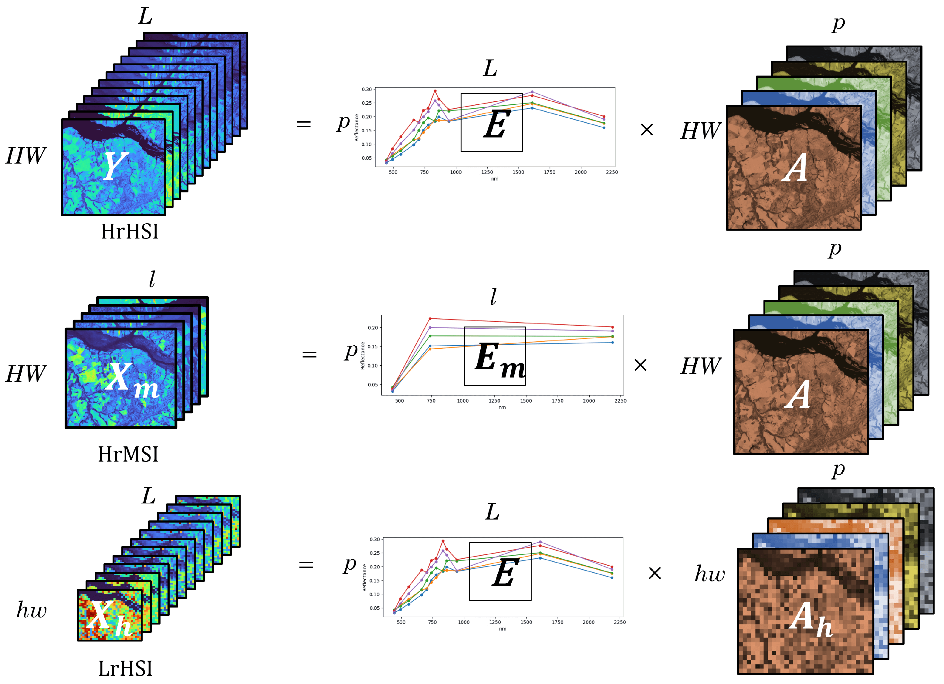
The main objective (target) of multispectral–hyperspectral data fusion is to estimate an output tensor combining high spectral and spatial resolutions. This is a generic problem described, for example, in [24,33,34]. This tensor is denoted as $\mathbf{Y}\in {\mathbb{R}}^{H\times W\times L}$, where H and W are the spatial dimensions and L is the spectral dimension. $\mathbf{Y}$ is also referred to as the High-Resolution Hyperspectral Image (HrHSI). The other “incomplete” data will be the High-Resolution Multispectral Image (HrMSI) and Low-Resolution Hyperspectral Image (LrHSI), denoted as ${\mathbf{X}}_m\in {\mathbb{R}}^{H\times W\times l}$ and ${\mathbf{X}}_h\in {\mathbb{R}}^{h\times w\times L}$, respectively. h, w, and l represent the low spatial and spectral resolutions. According to the Linear Mixing Model (LMM), we can establish a relationship between $\mathbf{Y}$, ${\mathbf{X}}_h$ and ${\mathbf{X}}_m$. The LMM assumes that every pixel of a remote sensing image is a linear combination of pure spectral entities/signatures, often called endmembers. In a linear dependency, these endmembers have coefficients, also referred to as abundances. For each pixel, the linear model is written as follows (c.f. [35]):

$$y_i=\sum _{j=1}^q{e}_{ij}{\alpha }_j+n_i$$

(1)

where

• $y_i$ is the reflectance at spectral band i,
• $e_{ij}$ is the reflectance of the endmember j at band i,
• ${\alpha }_j$ is the fractional abundance of j,
• $n_i$ is the error for the spectral band i (i.e., noise etc).

Equation (1), written in vector form, minus the error term (assuming perfect acquisition for simplicity, is expressed as:

$$\mathit{Y}=\mathit{E}\mathit{A}$$

(2)

Similarly, for LrHSI,

$${\mathit{X}}_h=\mathit{E}{\mathit{A}}_h$$

(3)

with the same spectral signatures as Y but with lower spatial resolution. Hence, the matrix ${\mathit{A}}_h\in {\mathbb{R}}^{h\times w\times p}$, with p being the number of endmembers, consists of $a_{ij}^s$ low-spatial-resolution coefficients.

The HrMSI will have the same properties but with the opposite degradation,

$${\mathit{X}}_m={\mathit{E}}_m\mathit{A}$$

(4)

where ${\mathit{E}}_m\in {\mathbb{R}}^{p\times l}$ is the endmembers matrix, with p being the number of spectral signatures and l being the number of spectral bands.

The LrHSI can be considered as a spatially degraded version of the HrHSI written as:

$${\mathit{X}}_h=\mathit{Y}\mathit{S}$$

(5)

with $\mathit{S}\in {\mathbb{R}}^{hw\times HW}$ as the spatial degradation matrix, referring to the downsampling and blurring operations. Furthermore, $\mathit{R}\in {\mathbb{R}}^{L\times l}$ can be considered as the spectral degradation matrix, giving:

$${\mathit{X}}_m=\mathit{Y}\mathit{R}$$

(6)

${\mathit{Z}}_{lr}\in {\mathbb{R}}^{h\times w\times l}$ represents the LrMSI.

The dependencies between HrHSI ($\mathbf{Y}$), HrMSI (${\mathit{X}}_m$), and LrHSI (${\mathit{X}}_h$) are illustrated in Figure 2.

From a deep learning point of view, the objective is thus to find the non-linear mapping $f_{\mathsf{\Theta }}(·)$, referred to as our neural network, which gives us an approximation of Y given ${\mathit{X}}_h$ and ${\mathit{X}}_m$, called our prediction $\widehat{\mathit{Y}}$.

$$\begin{array}{c}\hfill \widehat{\mathit{Y}}=f_{\mathsf{\Theta }}({\mathit{X}}_h,{\mathit{X}}_m)\end{array}$$

(7)

$$\begin{array}{c}\hfill \mathrm{with}\widehat{\mathit{Y}}\simeq \mathit{Y},\end{array}$$

(8)

and with $\mathsf{\Theta }$ being the network parameters. In this context, the S2 image is analogous to the HrMSI and the S3 image to the LrHSI. The HrHSI refers to the Ground Truth.

3. Materials

When tackling the fusion task with a DL approach, a major challenge emerges, the absence of ground truth. It is necessary, when training a neural network, to compare the current prediction to a reference in order to calculate the difference between the two and subsequently update the model weights. This process, known as back-propagation [36], allows the neural network to update its parameters and converge towards the minima. Concerning the Sentinel-2 and 3 missions, there is no image available already combining the full LrHSI spectral definition and the HrMSI spatial resolution. Section 3.1 presents our approach to obtaining a ground truth (GT) for training. The synthetic dataset generation is detailed in Section 3.3.

3.1. Ground Truth

To teach neural networks to fuse HrMSI and LrHSI, a ground truth (GT) is needed that combines the high spatial and high spectral resolutions (see Section 2). Datasets of this kind are available in the context of EO, such as the Urban dataset [37], the Washington DC Mall dataset [38], and the Harvard dataset [39]. However, the main challenges with these are their limited sizes, sometimes covering less than a kilometer, and their spectral ranges, which, in most cases, do not encompass the extended range offered by S2 and S3.

Because our objective is to generate physically accurate data, we need a training dataset with the right spectral coverage, diverse images, and large enough areas covered. To remedy the lack of appropriate data, specifically prepared and/or complete synthetic datasets are needed.

In this study, the main approach was to synthetically generate Sentinel-2 and Sentinel-3 approximations, together with a ground truth using representative hyperspectral data. Section 3.3 describes the procedure in detail and portrays the deep learning training process. It also shows limitations due to the theoretical spatial definition obtained from the input data and the spectral range. This approach can be characterized as an attempt to get as close as possible to reality and make the neural network learn the physics behind the Sentinel sensors.

An alternative approach to compensate for the weaknesses of the above method was also explored (Section 3.4). This approach involves using a well-known dataset for hyperspectral unmixing and data fusion, transforming it, and analyzing the network’s performance on EO image fusion. Specifically, we use the multispectral CAVE dataset [40]. These input data enable us to push the theoretical limits of spatial resolution in fusion and to test the network’s ability to generalize data fusion beyond the EO context. Based on the detailed performance evaluations of the EO-trained network presented in Section 5 and Section 6, readers should consider the CAVE-trained architecture as a benchmark reference. This comparison facilitates an in-depth analysis of our synthetic training approach by providing a reference point against alternatives derived from a more generic image fusion dataset. By doing so, readers can better understand the relative efficacy and benefits of our synthetic training method in contrast to more conventional approaches.

3.2. Input Multi-Spectral Data

3.2.1. Satellite Imagery

• Sentinel-2
  The Sentinel-2 MultiSpectral Instrument (MSI) gathers data across 12 spectral bands, spanning from visible to shortwave infrared wavelengths (412 nm to 2320 nm).
  The MSI product proposes reflectance values (the HrMSI) at spatial resolutions from 10 to 60 m. The image is atmospherically corrected and orthorectified at 2A level (L2A) [41].

• Sentinel-3
  The Sentinel-3 SYNERGY products include 21 spectral bands (from 400 nm to 2250 nm) at a 300 m GSD, combining data from two optical instruments: the Ocean and Land Color Instrument (OLCI) and the Sea and Land Surface Temperature Radiometer (SLSTR). The LrHSI. Like Sentinel-2, the gathered data type is in reflectance values, L2A atmospherically corrected and orthorectified.
  In this study, we used the Copernicus Browser (https://browser.dataspace.copernicus.eu, accessed on 14 August 2024) to retrieve overlapping S2 and S3 image pairs with acquisition times within 5 min of each other and with a cloud coverage fraction of a maximum of 5%.

• EnMAP
  EnMAP is a satellite mission dedicated to providing high-resolution, hyperspectral Earth Observation data for environmental and resource monitoring purposes. EnMAP’s spectrometer captures detailed spectral information across 246 bands, going from 420 nm to 2450 nm. The satellite has a 30 km swath width at a GSD of 30 m, with a revisit time at nadir of 27 days and 4 days off-nadir. The spectral resolution is significantly more detailed than Sentinel-2 MSI (12 bands) and Sentinel-3 SYNERGY (21 bands), and the GSD is 3 times below S2 but 10 times better than S3, giving us a good compromise for our experimentation.

3.2.2. CAVE

The CAVE dataset consists of a diverse array of interior scenes featuring various physical objects, captured under different lighting conditions using a cooled CCD camera. This dataset does not include any Earth Observation images but is a well known and commonly used dataset in multi-spectral image fusion ([25,42,43]). The images comprise 31 spectral bands ranging from blue to near-infrared (400 nm to 700 nm).

Figure 3 illustrates a typical example from the CAVE dataset, showing an image of a feather alongside its mean spectral curve, which represents the average values across all 31 bands. This provides a more comprehensive perspective of the scene compared to conventional RGB imaging.

3.3. Synthetic EO Dataset Preparation

Synthetic S2 and S3 training data, as well as ground truth data (for the fusion product), were prepared using real hyperspectral satellite imagery (with hundreds of spectral channels and GSD of 30 m or better) obtained with the Environmental Mapping and Analysis Program (EnMAP) satellite ([44]).

The EnMAP imagery, like S2 and S3, is also in reflectance values, L2A atmospheric correction, and orthorectified. Because the acquisition hardware is a spectrometer, EnMAP gives us access to the true spectrum of the area being captured. EnMAP hyperspectral datawere retrieved from the EnMAP GeoPortal (https://eoweb.dlr.de/egp/main, accessed on 14 August 2024). We selected a variety of representative EO images (e.g., biomes and terrains) to have a representative and diverse training dataset. This optimizes the possibility of training the neural network with an optimized variance. The location of the 159 selected hyperspectral images is shown in Figure 4. The approximate width of all the images is around 30 km. The number of requested images per continent is given in Appendix A.1.

Synthetic S2 and S3 products were derived from the EnMAP high-resolution spectra by convolving with each of the S2 and S3 spectral response functions (SRFs) provided by the European Space Agency (https://sentinels.copernicus.eu/web/sentinel/user-guides/sentinel-2-msi/document-library/-/asset_publisher/Wk0TKajiISaR/content/sentinel-2a-spectral-responses, accessed on 14 August 2024) as per Equation (9) (Chander et al. [45]):

$$\overline{{\rho }_{\lambda }}={\displaystyle \frac{\int {\rho }_{\lambda }\times SR{F}_{\lambda }d\lambda }{\int SR{F}_{\lambda }d\lambda }},$$

(9)

with $\overline{{\rho }_{\lambda }}$ being the product of the integrated SRF and spectrum at the band $\lambda$ position.

Figure 5 shows an example EnMAP spectrum together with the MSI, OLCI, and SLSTR SRF curves. An example of the resulting synthetic MSI images is given in Figure 6.

A limitation remains: Sentinel-3 has a spectral range going farther into the blue part of visible light, going beyond the capabilities of the EnMAP data’s spectral range. Hence, the first 2 bands could not be simulated, resulting in S3 and ground truth spectra with 19 bands.

After simulating all bands for all products, two synthetic tensors are generated from each EnMAP spectral cube:

• A Sentinel-2 MSI simulation, 12 bands, 30 m GSD;
• A Sentinel-3 SYNERGY simulation, 19 bands, 30 m GSD.

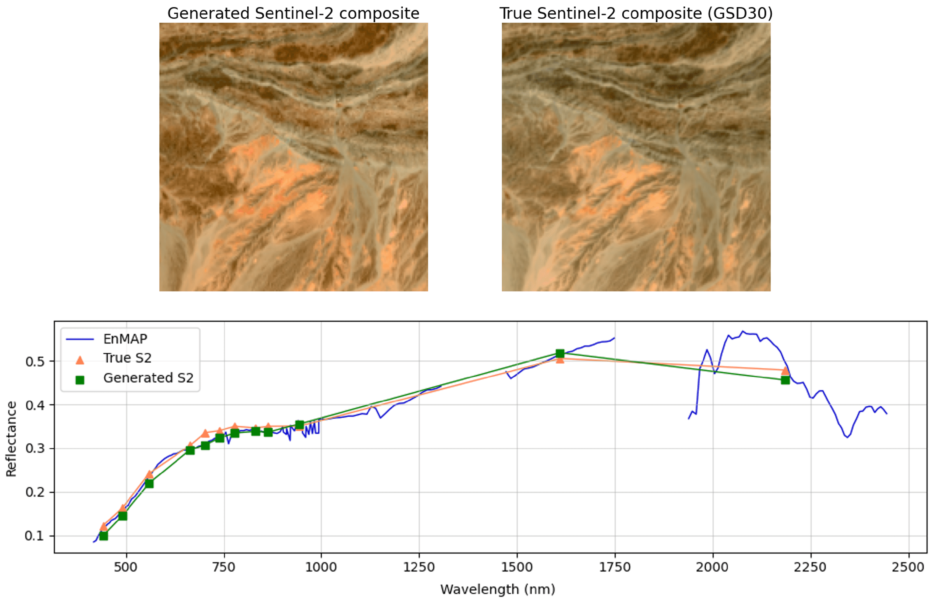
To check the fidelity of our synthetic S2 and S3 data, we compared them against true observed S2 and S3 data for areas that are covered by both EnMap and Sentinel instruments. The synthetic and true images are compared using the Spectral Angle Mapper (SAM) and the Structural Similarity Index (SSI). We show in Figure 7 an example of a pair of synthetic S2 data against corresponding S2 observations, as well as the corresponding EnMap, synthetic, and true spectra. We managed to check the sanity of the ground truth for over 80 percent of the pixels used in the training, validation, and testing sets, and never found values of SAM or SSI indicative of strong deviations between the synthetic and the true S2 and S3 images and spectra, where strong deviation could have been detected via a SAM with values above 0.1, and an SSI with values below 0.8.

This technique allows us to create a Sentinel-3 image with 10 times better spatial resolution; this datacube will be considered as our ground truth. To retrieve the true Sentinel-3 GSD from it, we apply a 2D Gaussian filter, degrading the spatial resolution to 300 m (The Gaussian filter acts as a low-pass filter in the frequency domain, efficiently eliminating high-frequency components that are unnecessary at lower resolutions. In essence, the 2D Gaussian filter is used for its ability to smooth, reduce noise, and preserve image integrity during significant resolution changes).

It is important to recognize that this approximation will never be perfect due to intrinsic differences between the S2 and EnMAP instruments that are not fully addressed by integrating the SRF, such as the calibration of the instruments. However, we are confident that the fidelity of our synthetic datasets is high when compared to the true data. Additionally, there are inherent limitations due to the theoretical spatial definition derived from the input data (30 m). The simulated data, while providing a close approximation, may not completely capture the fine spatial details present in real-world observations (10 m). However, given the diversity and pertinence of the data used, we believed that the network would be able to generalize sufficiently to overcome these limitations. The results (Section 5) show predictions performed at the training resolution for consistency. Going further, the training GSD is described in the discussion (Section 6). Nonetheless, further refinement and validation against real-world data could be necessary to enhance the accuracy and generalizability of the deep learning model; this aspect is not explored in this study.

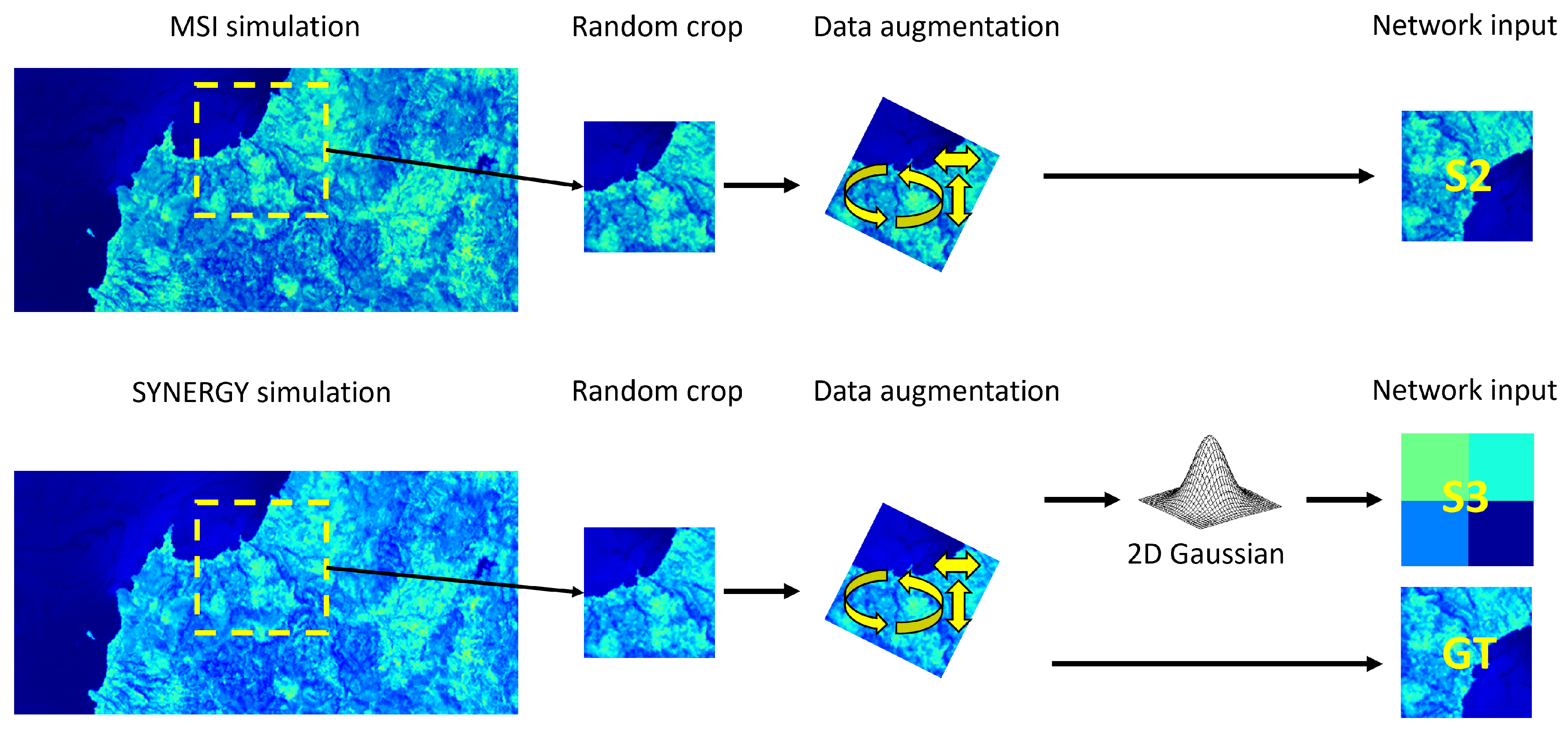
The data augmentation and preparation pipeline is summarized in the dataloader presented in Figure 8. From this, 10,000 S2/S3/GT image triplets were extracted and used as our training dataset.

3.4. Synthetic Non-EO (CAVE) Dataset Preparation

The CAVE dataset was selected mainly for its popularity and variety. The use of the CAVE dataset as reference training serves as a portrayal of fusion examples made with a network trained on standard data.

There are two main challenges with this approach: the image spectral range does not match that of S2 and S3, and the scenes are non-EO. To tackle the first issue, data preparation is needed.

To align the spectral range of the CAVE images with that of the Sentinels, we used spline interpolation to enhance the spectral definition and adjust the output to match the Sentinel-2 and 3 spectral ranges. It is important to note that in this scenario, the data preparation is entirely synthetic, and the images do not represent actual EO observations, making it impossible to approximate the true responses of the Sentinels. Hence, unlike the preparation of EO data, all 21 bands were generated despite the spectral range of CAVE not aligning with that of the Sentinels.

The next step was to apply the same SRF integration techniques as in the previous section (i.e., Equation (9) to the CAVE spectra to generate synthetic S2 and S3 data. The same data preparation and augmentation steps (Figure 8) were applied to retrieve our HrMSI/LrHSI/HrHSI training and validating triplets (1000 images were extracted for training).

4. Method

4.1. The Neural Network

The neural network architecture selection was performed regarding specific criteria:

• Overall fusion performances on generic datasets: Neural networks trained on the fusion task have converged, most of the time, on generic datasets like CAVE. To the authors’ knowledge, no study has been conducted for performances on synthetic datasets like the one we have created (Section 3.3).
• The ability to generalize: Because of the synthetic nature of the training dataset, the training was carried out on images that do not perfectly fit reality. The neural network needs to have good generalization capabilities to apply the fusion process to diverse data.
• The number of network parameters: The fusion task is complex and involves massive inputs (images with 12 to 21 bands, thousands of pixels each); a network with a lot of parameters will inevitably involve massive computational times and potentially GPU memory overflow.

Neural networks have been historically used to tackle this task, like CNN-based networks: Guided-Net [46], originating from image super-resolution [47]; denoiser (CNN-FUS [48]); and many other architectures (e.g., [26,49,50]). Some very promising ones have emerged, wuch as CUCaNet [51] and Fusformer [52].

Fusformer was the selected architecture because of its high overall performance across all categories (accuracy, generalization capabilities, and parameter number). This network showed strong effectiveness at conventional fusions (on CAVE images for example) with rather fast training times (mainly due to the small number of parameters). This network uses a recent and effective deep learning technique, the Attention Mechanism, classifying it inside the Transformer network. A thorough explanation of this architecture is beyond the scope of this paper; here the main concepts behind Transformers networks are summarized.

In recent years, Transformer networks have significantly advanced AI in fields like natural language processing and computer vision. At the core of these models is attention, which allows networks to focus on specific input elements, mimicking human cognitive abilities. Originally introduced by [53] for natural language tasks, Transformers surpassed existing RNNs. This mechanism was later adapted in the Vision Transformer (ViT) for computer vision tasks [54]. Fusformer applied the ViT to the fusion task.

The Transformer block, inside Fusformer, is symbolized by the green block within the architecture in Figure 9.

4.2. Transformer Training

Regarding the synthetic EO dataset, Fusformer (where the implementation comes from the paper’s code repository, with no modification aside from the shape of the inputs and outputs) was trained for 150 epochs on 10,000 S2/S3/GT triplets with 1000 validation images. The calculation was carried out on an NVIDIA Geforce RTX 3090, 24MiB memory. To assess the performance of a fusion model, in the presence of ground truth, various metrics are employed, including Root Mean Square Error (RMSE), Peak Signal-to-Noise Ratio (PSNR), Error-Relative Global Absolute Scale (ERGAS), and Spectral Angle Mapper (SAM). All training and validation were performed using the Python programming language. All of these metrics are described in detail in Appendix B.

It is important to note that, contrary to typical RGB images, hyperspectral data are—for the same number of spatial pixels—more demanding in terms of GPU RAM. Thus the networks were trained on 20 m GSD for the Sentinel-2 images, dividing by 2 the pixel number. As an example, without downsampling S2, for an input S2 image of 150 × 150, the neural network processed 150 × 150 × 12 pixels for S2 and 150 × 150 × 21 for S3. Figure 9 shows that Sentinel-3 is upsampled to match the Sentinel-2’s shape, giving us 742,500 pixels to compute for an image of just 150 × 150 pixels. Because of the extensive memory load, the batch size was set to 1. The learning rate was left to its default value, from the original Fusformer code, at $1\times {10}^{-3}$ with a weight decay set at .1 at all 30 epochs. In addition to the high variety of the training dataset, which drastically lowers the overfitting problem (particularly in front of synthetic data), a dropout rate was added and fixed to 0.2.

Figure 10 and

Table 1. Training metrics’ start and end values, 150 epochs. Arrows next to the metric indicate whether the metric needs to decrease (↓) or increase (↑).

Metric	Epoch 1	Epoch 150
MSE train (↓)	0.036	0.003
MSE val (↓)	0.032	0.003
RMSE (↓)	0.053	0.006
ERGAS (↓)	1.135	0.129
SAM (↓)	13.976	1.152
PSNR (↑)	22.134	43.456
Single band fusion
	Band 18	Band 18

show the convergence of metrics with an example of better spatial features definition throughout training.

5. Results

In this section, we present contextual S2 and S3 fusions. By contextual, we mean that the input images are true S2 and S3 images coming from the Copernicus request hub, and the following results demonstrate the network capabilities on non-synthetic images.

We apply the models obtained in the previous section to real S2 and S3 multispectral images to obtain new S2-S3 fusion products.

Inference Results—Natural-Color Composite Images and Spectra

In Section 4.2, we explain that because of computing power limitations, the input S2 images (CAVE training) were downgraded to a GSD of 20 m. For the input data, there is a resolution factor of 15 between the HrMSI and the LrHSI. In the case of the EO training, the native EnMAP resolution is 30 m GSD (Section 3.3), hence restricting the input resolution difference to a factor 10. For consistency, the figures and metrics presented in this section are performed with the same resolution factor as seen in training.

In contrast to the training with the EnMAP-based ground truth, the CAVE training set offers a theoretically “infinite” spatial resolution for Earth Observation data, with interior scene resolution reaching approximately millimeter-level precision. Despite being trained on unrelated data, the primary expectation for network generalization was that the Transformer could still effectively transfer spatial features, as certain elements within the CAVE images have resemblances to EO features.

Figure 11 (top panel) shows four RGB composites with the following bands:

• S3: 4, 7, 10 (490 nm, 560 nm, 665 nm)
• S2: 2, 3, 4 (490 nm, 560 nm, 665 nm)
• AI fused: 4, 7, 10 for CAVE trained and 2, 5, 8 for EO trained (see Section 3.3 for the two missing bands)

The bottom panel displays the mean spectra for all images with standard deviation at each band.

Table 2. Inference metrics calculated for the fused products shown in Figure 11 (Angola) using the non-EO (CAVE) and EO training data respectively. The best results are underlined. Metrics that need to be maximized are noted (↑), best is 1. Metrics that need to be minimized are noted (↓), best is 0.

Metric	EO	CAVE
J-S Divergence (↓)	0.032	0.065
SAM (↓)	0.013	0.085
SSI (↑)	0.988	0.988

shows the metrics presented in Appendix C. Please note that the Inception Score is unavailable for these tests. This is due to the classifier being trained on 10 m GSD images, making it unsuitable for handling predictions at 20 m or 30 m.

Several metrics are used to assert the accuracy of the inference. One major difference is that unlike during training, we do not have access to a ground truth; therefore, all of the previously used metrics (Section 4.2) cannot be calculated anymore. For the inference, we use three different metrics, the Jensen–Shannon Divergence, SAM, and SSI. Note that here, the SSI is calculated on the downgraded S2 panchromatic image to 20 m for CAVE and 30 m for EO. More details for each of these metrics are given in Appendix C.

These first results show that the EO-trained Transformer fits the S3 mean spectrum with around the same standard deviation values. This behavior is expected (reconstructed images with the S3 spectrum and the S2 GSD). Slight differences can be witnessed between the AI fused product and the S2 composites, which are explained by the intrinsic deviations from the S2 and S3 spectra. Although the bands used to create the composites are at the same wavelength, they do not always have the same responses due to some disparities: different instruments, calibration, visit time, filter width, etc. The SSI (Table 2) of 0.988 (best is 1) reflects a good reconstruction of spatial features , usually slightly below the CAVE training, which seems to perform better overall in fine-grain detail transfer (potentially explained by the CAVE images’ millimeter-level resolution). The composite colors will most of the time be closer to the S2 image; the underlying cause of this is that the CAVE-trained model tends to reconstruct spectra closer to the S2 reflectance than S3, leading to significantly lower metrics in the spectral domain (2 times lower J-S Divergence and around 6 times lower SAM).

The white square on the S2 composite, Figure 11, is zoomed in on in Figure 12; the comparison is made on a 30 m GSD for S2 to truly show the fusion accuracy with the given spatial information at the inference time.

Examples like Figure 13 show significant spectral deviations coming from the CAVE-trained network; such deviations were not observed on the EO-trained Transformer.

The CAVE dataset spectra tend to be flat due to the scene’s chemical composition. The network has difficulties reconstructing spectra deviating from the examples seen throughout training (e.g., Figure 13) where the mean spectra bump around 700 nm, a common behavior when dealing with dense chlorophyll emission (called “red edge”). The CAVE-trained network’s spectral accuracy drastically decreases in these situations (also shown in

Table 3. Inference metrics calculated for the fused products shown in Figure 13 (Amazonia) using the non-EO (CAVE) and EO training data, respectively. The best results are underlined. Metrics that need to be maximized are noted (↑), best is 1. Metrics that need to be minimized are noted (↓), best is 0.

Metric	EO	CAVE
J-S Divergence (↓)	0.051	0.502
SAM (↓)	0.020	0.278
SSI (↑)	0.900	0.967

).

In the case of the Amazonia zoomed-in area, shown in Figure 14, some spatial features were not accurately reconstructed, e.g., the cloud shadow in the upper-left corner. One explanation could be that the neural network was trained on almost cloudless data. Including more (partially) cloudy images in the training dataset could perhaps give better results.

We stress that Sentinel-2 and Sentinel-3 images cannot be taken at the exact same time, which can lead to potential spatial discrepancies between the two. To address this, we selected the closest possible acquisition dates for both the S2 and S3 images, operating under the assumption that a 5 min difference is insufficient for significant spatial changes to occur. However, if the image acquisition times are significantly different, users should be aware that the network may reconstruct spatial features that are not present in one of the input images.

These results lead to the following conclusions on the trained networks:

• Both networks can perform data fusion at the training GSD (30 m).
• The CAVE-trained Transformer has slightly better spatial reconstructions at the training GSD.
• The CAVE-trained network fused spectra stick to Sentinel-2, while the EO network sticks to Sentinel-3.
• The spectral reconstruction capability of the EO-trained Transformer surpasses that of the other by several orders of magnitude.
• The EO network is more robust to diverse inputs and GSD (discussed in Section 6.
• The CAVE network showcased spatial and spectral “hallucinations” at 30 and 10 m. The EO-trained network remained stable.

6. Discussion

The results presented in the previous section (Section 5) demonstrated the accuracy of the network outputs in their training context. Here, we discuss the neural network’s ability to generalize beyond the training scope. Three particular cases are discussed. First, we show that it is possible to push the neural network to fuse images beyond the GSD seen during training (Section 6.1). Second, we discuss wide field predictions and Sentinel-3 image retrieval by degrading the fused outcome, allowing us to calculate distances and assert the deviation (Section 6.2). Thirdly, land cover segmentation is performed on both the fused and Sentinel-2 products to assess the impact on NDVI products (Section 6.3).

6.1. Inference (Fusion) beyond the Network Training Resolution

It became apparent, through testing, that it is possible to make the neural network fuse images with a smaller GSD than the one seen during training. The Transformer shows remarkable generalization capabilities and manages to transfer thinner spatial features to the bands to reconstruct. Figure 15 gives a fusion example for an urban scene (Los Angeles) with the maximum Sentinel-2 GSD (10 m). This example shows that the AI fusion not only generalizes well to higher spatial resolutions but also achieves good results for heterogeneous scenes (i.e., where the per-band standard deviation is high). The ability of the network to reconstruct scenes with fine-grained details and high variance at 10 m resolution is further illustrated in Figure 16.

Another way to investigate the network output’s imperfections is to analyze them in the frequency domain. Figure 17 shows the Discrete Fourier Transforms (DFTs) for the 665 nm band. Some recognizable features are missing in the AI-fused DFT compared to that of the Sentinel-2 one. Although the reconstruction has a good fidelity level in low frequencies, some structures are missing in medium and high magnitudes. This is highlighted in the difference plot at the right, extracting the pixels with the highest discrepancy. The network’s output is used as a highpass filter, summed with the up-scaled Sentinel-3 image afterward; it is natural to think that the main difficulty is to reproduce the frequencies necessary for sharp edges and fine-grain feature reconstruction. Improving the hyperparameters or implementing a deeper neural network architecture (more attention heads for example) might result in a better caching of medium and high frequencies for an improved fusion.

It is important to underline that the CAVE-trained Transformer has a better SAM metric than the EO-trained model (

Table 4. Metrics for the urban scene (Los Angeles) fusion shown in Figure 15. The best results are underlined. Metrics that need to be maximized are noted (↑), best is 1. Metrics that need to be minimized are noted (↓), best is 0. In the case of the IS, no finite upper limit is defined.

Metric	EO	CAVE
J-S Divergence (↓)	0.095	0.102
SAM (↓)	0.079	0.065
SSI (↑)	0.989	0.953
IS (↑)	1.245	1.264

) but shows spatial feature “hallucinations” (colored pixels unrelated to the surroundings) not seen in the latter. This behavior is shown in Figure 18 where the hallucinations are highlighted (cf. Figure 19 for a close-up). This effect was not encountered with the EO-trained Transformer (leading to a much higher SSI value, as shown in

Table 5. Fused product metrics (France). The best results are underlined. Metrics that need to be maximized are noted (↑), best is 1. Metrics that need to be minimized are noted (↓), best is 0. In the case of the IS, no finite upper limit is defined.

Metric	EO	CAVE
J-S Divergence (↓)	0.123	0.321
SAM (↓)	0.011	0.136
SSI (↑)	0.961	0.512
IS (↑)	3.589	3.377

). A potential explanation comes from the fact that the EO-trained dataset is much larger and more diverse than the CAVE one, making generalization easier.

In summary, The EO-trained network globally showed the ability to reconstruct spatial features at 10 m GSD, like Figure 11, a close-up example at Figure 12, and the same zoomed-inarea at GSD 10 m shown in Figure 20. Additional fusion examples are given in Appendix F, using the EO-trained neural network only, to illustrate, for instance, the spatial and spectral variety of scenes.

6.2. Wide Fields and Pseudo-Invariant Calibration Sites

An extension of the above analysis is to conduct fusions on wide images covering several kilometers (getting closer to the true Sentinel-2 and 3 swaths). From these broad fusions, it is possible to retrieve a Sentinel-3-like image by intentionally degrading the result. By doing so, we can calculate the distance measures from the degraded output and the true Sentinel-3 image.

For these comparisons, we have selected areas included in the Pseudo-Invariant Calibration Sites (PICSs) program ([55,56,57]). These regions serve as terrestrial locations dedicated to the ongoing monitoring of optical sensor calibration for Earth Observation during their operational lifespan. They have been extensively utilized by space agencies over an extended period due to their spatial uniformity, spectral stability, and temporal invariance. Here, we chose two sites, Algeria 5 (center coordinates: N 31.02, E 2.23, area: 75 × 75 km) and Mauritania 1 (center coordinates: N 19.4, W 9.3, area: 50 × 50 km).

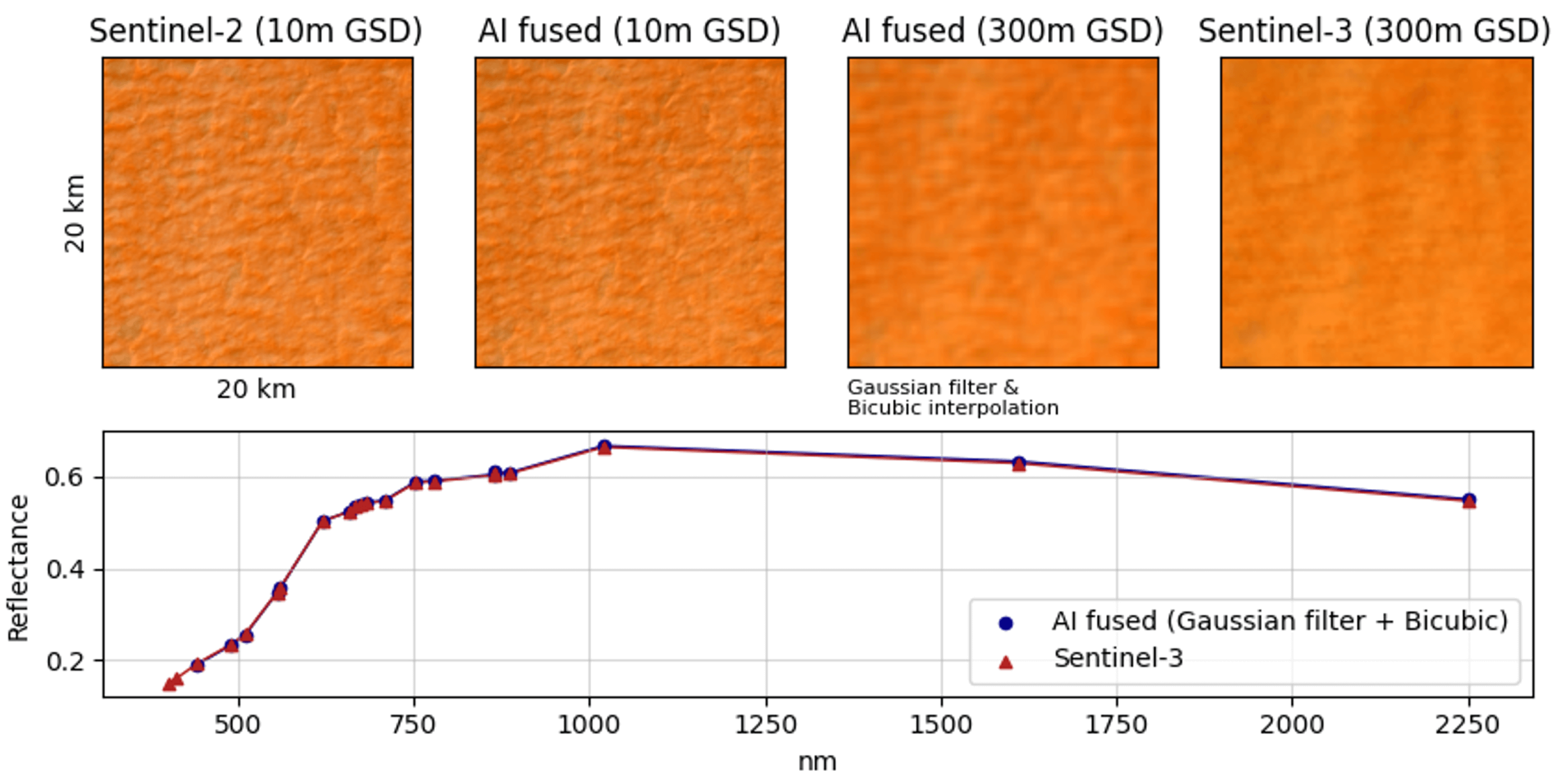
It is mportant to note that this is not an iterative process; the Sentinel-3 image is indeed among the network’s input. It would be natural to think that degrading the output to retrieve an input-like image is a regressive endeavor. However, this is carried out mainly to show that we are not deviating significantly from the original spectral data. To approximate the Sentinel-3 GSD, we first convolve the HrHSI with a Gaussian filter and then pass it through a bicubic interpolation. The Gaussian kernel and the interpolation are defined in Appendix D.

The main interest of this process is to go back to our original Sentinel-3 image, giving us the possibility to use a GT to determine the distance between the Sentinel-3 and the degraded fusion result. The metrics used are the RMSE, Euclidean distance, and cosine similarity (cf.

Table A1. Metrics used to determine the distance between Sentinel-3 and the degraded fusion.

Metric	Formula
RMSE	$\sqrt{{\displaystyle \frac{1}{n}}{\sum }_{i=1}^n{(y_i-{\widehat{y}}_i)}^2}$
Euclidean distance	$\sqrt{{\sum }_{i=1}^n{(x_i-y_i)}^2}$
Cosine similarity	${\displaystyle \frac{\mathbf{x}·\mathbf{y}}{\parallel \mathbf{x}\parallel ·\parallel \mathbf{y}\parallel }}$

).

All of the following fusions are performed with the EO-trained network, mainly because its mean spectra are closer to Sentinel-3, leading to better results when trying to retrieve GSD 300 SYNERGY.

Because we cannot infer images this big, the fusion was performed using mosaic predictions, with 150 × 150-pixel sub-images with a 20-pixel margin overlap; for Figure 21 and Figure 22, predictions for the 256 sub-images were carried out in 2:41 min.

Figure 21. Twenty-kilometer-wide GSD 10 m and 300 M fused product inside the Algeria CEOS zone (top panels). The Sentinel-3 and GSD 300 AI fused image mean spectra are also displayed in the bottom panel. The corresponding metrics for this inference are in

Table 6. Metrics calculated on the interpolated fusion and the Sentinel-3 image (CEOS Algeria). Metrics that need to be maximized are noted (↑), best is 1. Metrics that need to be minimized are noted (↓), best is 0.

Metric	Value
RMSE (↓)	0.011
Euclidean distance (↓)	3.403
Cosine similarity (↑)	0.999

.

Figure 21. Twenty-kilometer-wide GSD 10 m and 300 M fused product inside the Algeria CEOS zone (top panels). The Sentinel-3 and GSD 300 AI fused image mean spectra are also displayed in the bottom panel. The corresponding metrics for this inference are in Table 6.

Figure 22. Twenty-kilometer-wide GSD 10 and 300 fused products inside the Mauritania CEOS zone. The Sentinel-3 and GSD 300 AI fused image mean spectra are also displayed in the second row. Metrics for this inference are displayed

Table 7. Metrics calculated on the interpolated fusion and the Sentinel-3 image (CEOS Mauritania). Metrics that need to be maximized are noted (↑), best is 1. Metrics that need to be minimized are noted (↓), best is 0.

Metric	Value
RMSE (↓)	0.01430
Euclidean distance (↓)	4.239
Cosine similarity (↑)	0.999

.

Figure 22. Twenty-kilometer-wide GSD 10 and 300 fused products inside the Mauritania CEOS zone. The Sentinel-3 and GSD 300 AI fused image mean spectra are also displayed in the second row. Metrics for this inference are displayed Table 7.

Other wide fields were tested, and some of them were selected for their dense and varied spatial features, like in urban areas. A typical example is depicted in Figure 23.

This inference took 37 s for 64 mosaic sub-images. The metrics are listed in

Table 8. Metrics calculated on the interpolated fusion and the Sentinel-3 image (Los Angeles). Metrics that need to be maximized are noted (↑), best is 1. Metrics that need to be minimized are noted (↓), best is 0.

Metric	Value
RMSE (↓)	0.016
Euclidean distance (↓)	2.463
Cosine similarity (↑)	0.996

.

To conclude this section on wide fields, we show visually (with RGB composites) and with distance metrics that degrading the fused product to simulate a 300 m GSD gives only a small deviation from the true Sentinel-3 data, e.g., with SSI and cosine similarity always close to the best value (best is 1).

6.3. Normalized Difference Vegetation Index Classifications

Through a comparative analysis, we can evaluate the non-regression of our network and ensure that accuracy is maintained between Sentinel-2 and the fused product at 10 m. The Normalized Difference Vegetation Index (NDVI) is a numerical indicator used in remote sensing to assess vegetation health and density. It measures the difference between NIR and red light reflectance, providing insights into vegetation health and biomass. It can also easily distinguish green vegetation from bare soils. NDVI values typically span from −1.0 to 1.0. Negative values signify clouds or water areas, values near zero suggest bare soil, and higher positive NDVI values suggest sparse vegetation (0.1–0.5) or lush green vegetation (0.6 and above) ([58,59]). Using our trained neural network and a segmentation ground truth over a specific area, it is possible to compare the NDVIs derived from both the fused and Sentinel-2 products with the classification GT. For the fused product, we benefit from the Sentinel-3 spectral bands to compute the NDVI. We recall that the main difference between the Sentinel-2 NDVI and the Sentinel-3 NDVI is that, from the NDVI definition, $\left[\left({\rho }_N-{\rho }_R\right)/\left({\rho }_N+{\rho }_R\right)\right]$, where ${\rho }_N$ is the pixel reflectance value at NIR and ${\rho }_R$ is the pixel reflectance value at red wavelength, we can combine Sentinel-3 bands to extract the NIR and red factors. This process is not possible with Sentinel-2 due to its sparse spectra. For the AI-fused product, we used the mean value of the bands 15, 14, and 13 to collect the NIR reflectance and the bands 8, 7, and 6 mean value for the red reflectance. For Sentinel-2, only one band was used for the NIR (band 7), and one for the red (band 3). Figure 24 shows the NDVI matrices derived from the AI fused (EO trained) and Sentinel-2 products. Both are compared to the area ground truth, retrieved from the Chesapeake dataset [60].

The error is assessed by performing a Jaccard score calculation, commonly used in classification accuracy measurements [61]. It calculates the absolute values of the intersection of the two classified sets (let A be the predicted NDVI and B the GT) over their union, defined as

$$\mathcal{J}(A,B)={\displaystyle \frac{|A\cap B|}{|A\cup B|}}={\displaystyle \frac{|A\cap B|}{\left|A\right|+\left|B\right|-|A\cap B|}}$$

(10)

Note that, even though the retrieved Sentinel-2 and Sentinel-3 images are close in time to the ground truth acquisition time, they do not perfectly overlap. This can lead to slight differences between observed elements and the GT statements. The Jaccard score was calculated regardless of this de-synchronization. The Jaccard score for the AI-fused product is 0.340, while the Sentinel-2 score is 0.337 (the best score is 1). Despite being minor, the variance in accuracy underscores a slight improvement achieved with the fused product, primarily attributed to the enhanced spectral definition, facilitating the collection of additional information. Another example is shown in Figure A2.

7. Summary and Conclusions

In this study, we presented a new DL methodology for the fusion of Sentinel-2 and Sentinel-3 images utilizing existing hyperspectral missions, particularly EnMAP, to address the absence of varied ground truth images in the Earth Observation image fusion discipline. Our approach aimed to reconstruct images embedding the Sentinel-3 spectra along the Sentinel-2 spatial resolution. To this end, we customized an existing Transformer-based neural network architecture, Fusformer.

To emphasize the importance of using contextual data, we trained our neural network using two distinct training and validation datasets. For the first training set, we created a synthetic contextual reference dataset, including ground truth, using a large variety of hyperspectral EnMAP images. In the second training, we used the CAVE database, consisting of multi-spectral images of interior scenes, to create a generic, non-EO-specific, training and validation training set. This comparison is also useful since the CAVE data are ubiquitously used for bench-marking (multi-/hyperspectral) image fusion and super-resolution algorithms.

Through comprehensive experimentation and evaluation, we observed notable differences in the performance of the two neural networks when applied to the tasks of Sentinel-2 and Sentinel-3 image fusion. The network trained on the synthetic EO dataset outperformed its counterpart trained on non-EO data across various evaluation metrics. In particular, inference with the non-EO model gave rise to “hallucinations”, pixels showing erratic spectral behavior not seen for the EO contextual model. Furthermore, our selected neural network demonstrated the potential to fuse Sentinel-2 and Sentinel-3 images beyond the spatial resolution encountered during training. Despite this resolution disparity, our approach extended the fusion capabilities to higher resolutions, showcasing its adaptability and robustness in handling varying spatial scales inherent in Earth Observation data. Inference on wide fields and Pseudo-Invariant Calibration gave excellent results, which is a first step towards an operational implementation of S2-S3 data fusion. Lastly, we looked at a practical example, NDVI classification, to illustrate how S2-S3 fusion products could potentially improve EO applications and services.

Our findings highlight the potential and importance of generating synthetic contextual (EO) training input, as well as the Transformer-based neural networks, to improve the fusion of multi-spectral remote sensing observations. Hyperspectral missions can play a key role in providing necessary ground truth.

This approach not only facilitates the integration of complementary information from different satellite sensors but also contributes to advancing the capabilities of EO data analysis and interpretation. However, limitations do exist.

The study’s limitations are primarily rooted in the synthetic nature of the training data, which introduces biases that may not fully capture real-world fusion scenarios. Moreover, the reliance on Sentinel-2 and Sentinel-3 image pairs with small temporal differences restricts the broader applicability of the methodology, as it diminishes the potential for fusing images with larger temporal gaps. Finally, due to the lack of true ground truth data, it remains challenging to definitively validate the results at the Sentinel-2 ground sample distance (GSD) of 10 m, leaving some uncertainty about the model’s accuracy and effectiveness. Nonetheless, the approach demonstrates significant promise by showcasing the capabilities of multi-spectral fusion using deep neural networks trained on synthetic datasets, potentially enhancing EO application and demonstrating the potential for further advancements in EO data analysis and interpretation.

Training on synthetic data, even when sourced from a different instrument from those used at inference, presents an opportunity to enhance models. Further research is necessary to maximize the performance and scalability of both the data augmentation and preparation pipeline and the network architecture itself. Additionally, generalizing our approach across different EO missions and platforms could provide valuable insights into its broader applicability and potential for improving the synergy between existing and future Earth Observation systems.

References

1. Du, Y.; Song, W.; He, Q.; Huang, D.; Liotta, A.; Su, C. Deep learning with multi-scale feature fusion in remote sensing for automatic oceanic eddy detection. Inf. Fusion 2019, 49, 89–99. [Google Scholar] [CrossRef]
2. Nguyen, H.; Cressie, N.; Braverman, A. Spatial statistical data fusion for remote sensing applications. J. Am. Stat. Assoc. 2012, 107, 1004–1018. [Google Scholar] [CrossRef]
3. Chang, S.; Deng, Y.; Zhang, Y.; Zhao, Q.; Wang, R.; Zhang, K. An advanced scheme for range ambiguity suppression of spaceborne SAR based on blind source separation. IEEE Trans. Geosci. Remote Sens. 2022, 60, 1–12. [Google Scholar] [CrossRef]
4. Jutz, S.; Milagro-Perez, M. Copernicus: The European Earth Observation programme. Rev. De Teledetección 2020, 56, V–XI. [Google Scholar] [CrossRef]
5. Gomez, C.; Viscarra Rossel, R.A.; McBratney, A.B. Soil organic carbon prediction by hyperspectral remote sensing and field vis-NIR spectroscopy: An Australian case study. Geoderma 2008, 146, 403–411. [Google Scholar] [CrossRef]
6. Carter, G.A.; Lucas, K.L.; Blossom, G.A.; Lassitter, C.L.; Holiday, D.M.; Mooneyhan, D.S.; Fastring, D.R.; Holcombe, T.R.; Griffith, J.A. Remote Sensing and Mapping of Tamarisk along the Colorado River, USA: A Comparative Use of Summer-Acquired Hyperion, Thematic Mapper and QuickBird Data. Remote Sens. 2009, 1, 318–329. [Google Scholar] [CrossRef]
7. Okujeni, A.; van der Linden, S.; Hostert, P. Extending the vegetation–impervious–soil model using simulated EnMAP data and machine learning. Remote Sens. Environ. 2015, 158, 69–80. [Google Scholar] [CrossRef]
8. Fernández, J.; Fernández, C.; Féménias, P.; Peter, H. The copernicus sentinel-3 mission. In Proceedings of the ILRS Workshop, Annapolis, MD, USA, 10 October 2016; pp. 1–4. [Google Scholar]
9. Aziz, M.A.; Haldar, D.; Danodia, A.; Chauhan, P. Use of time series Sentinel-1 and Sentinel-2 image for rice crop inventory in parts of Bangladesh. Appl. Geomat. 2023, 15, 407–420. [Google Scholar] [CrossRef]
10. Grabska, E.; Hostert, P.; Pflugmacher, D.; Ostapowicz, K. Forest stand species mapping using the Sentinel-2 time series. Remote Sens. 2019, 11, 1197. [Google Scholar] [CrossRef]
11. Malenovský, Z.; Rott, H.; Cihlar, J.; Schaepman, M.E.; García-Santos, G.; Fernandes, R.; Berger, M. Sentinels for science: Potential of Sentinel-1, -2, and -3 missions for scientific observations of ocean, cryosphere, and land. Remote Sens. Environ. 2012, 120, 91–101. [Google Scholar] [CrossRef]
12. Toming, K.; Kutser, T.; Uiboupin, R.; Arikas, A.; Vahter, K.; Paavel, B. Mapping water quality parameters with sentinel-3 ocean and land colour instrument imagery in the Baltic Sea. Remote Sens. 2017, 9, 1070. [Google Scholar] [CrossRef]
13. Chen, C.; Dubovik, O.; Litvinov, P.; Fuertes, D.; Lopatin, A.; Lapyonok, T.; Matar, C.; Karol, Y.; Fischer, J.; Preusker, R.; et al. Properties of aerosol and surface derived from OLCI/Sentinel-3A using GRASP approach: Retrieval development and preliminary validation. Remote Sens. Environ. 2022, 280, 113142. [Google Scholar] [CrossRef]
14. Tarasiewicz, T.; Nalepa, J.; Farrugia, R.A.; Valentino, G.; Chen, M.; Briffa, J.A.; Kawulok, M. Multitemporal and multispectral data fusion for super-resolution of Sentinel-2 images. IEEE Trans. Geosci. Remote Sens. 2023, 61, 1–19. [Google Scholar] [CrossRef]
15. Vivone, G.; Restaino, R.; Licciardi, G.; Dalla Mura, M.; Chanussot, J. Multiresolution analysis and component substitution techniques for hyperspectral pansharpening. In Proceedings of the 2014 IEEE Geoscience and Remote Sensing Symposium, Quebec City, QC, Canada, 13–18 July 2014; pp. 2649–2652. [Google Scholar]
16. Loncan, L.; De Almeida, L.B.; Bioucas-Dias, J.M.; Briottet, X.; Chanussot, J.; Dobigeon, N.; Fabre, S.; Liao, W.; Licciardi, G.A.; Simoes, M.; et al. Hyperspectral pansharpening: A review. IEEE Geosci. Remote Sens. Mag. 2015, 3, 27–46. [Google Scholar] [CrossRef]
17. Selva, M.; Aiazzi, B.; Butera, F.; Chiarantini, L.; Baronti, S. Hyper-sharpening: A first approach on SIM-GA data. IEEE J. Sel. Top. Appl. Earth Obs. Remote Sens. 2015, 8, 3008–3024. [Google Scholar] [CrossRef]
18. Wei, Q.; Dobigeon, N.; Tourneret, J.Y. Bayesian fusion of multi-band images. IEEE J. Sel. Top. Signal Process. 2015, 9, 1117–1127. [Google Scholar] [CrossRef]
19. Zhang, Y.; De Backer, S.; Scheunders, P. Noise-resistant wavelet-based Bayesian fusion of multispectral and hyperspectral images. IEEE Trans. Geosci. Remote Sens. 2009, 47, 3834–3843. [Google Scholar] [CrossRef]
20. Zhang, Y.; De Backer, S.; Scheunders, P. Bayesian fusion of multispectral and hyperspectral image in wavelet domain. In Proceedings of the IGARSS 2008–2008 IEEE International Geoscience and Remote Sensing Symposium, Boston, MA, USA, 7–11 July 2008; Volume 5, p. V-69. [Google Scholar]
21. Dong, W.; Fu, F.; Shi, G.; Cao, X.; Wu, J.; Li, G.; Li, X. Hyperspectral image super-resolution via non-negative structured sparse representation. IEEE Trans. Image Process. 2016, 25, 2337–2352. [Google Scholar] [CrossRef] [PubMed]
22. Wei, Q.; Bioucas-Dias, J.; Dobigeon, N.; Tourneret, J.Y.; Chen, M.; Godsill, S. Multiband image fusion based on spectral unmixing. IEEE Trans. Geosci. Remote Sens. 2016, 54, 7236–7249. [Google Scholar] [CrossRef]
23. Zhang, K.; Wang, M.; Yang, S.; Jiao, L. Spatial–spectral-graph-regularized low-rank tensor decomposition for multispectral and hyperspectral image fusion. IEEE J. Sel. Top. Appl. Earth Obs. Remote Sens. 2018, 11, 1030–1040. [Google Scholar] [CrossRef]
24. Vivone, G. Multispectral and hyperspectral image fusion in remote sensing: A survey. Inf. Fusion 2023, 89, 405–417. [Google Scholar] [CrossRef]
25. Zhang, H.; Xu, H.; Tian, X.; Jiang, J.; Ma, J. Image fusion meets deep learning: A survey and perspective. Inf. Fusion 2021, 76, 323–336. [Google Scholar] [CrossRef]
26. Uezato, T.; Hong, D.; Yokoya, N.; He, W. Guided deep decoder: Unsupervised image pair fusion. In Computer Vision, Proceedings of the ECCV 2020: 16th European Conference, Glasgow, UK, 23–28 August 2020; Proceedings, Part VI; Springer: Cham, Switzerland, 2020; pp. 87–102. [Google Scholar]
27. Sara, D.; Mandava, A.K.; Kumar, A.; Duela, S.; Jude, A. Hyperspectral and multispectral image fusion techniques for high resolution applications: A review. Earth Sci. Inform. 2021, 14, 1685–1705. [Google Scholar] [CrossRef]
28. Yokoya, N.; Grohnfeldt, C.; Chanussot, J. Hyperspectral and multispectral data fusion: A comparative review of the recent literature. IEEE Geosci. Remote Sens. Mag. 2017, 5, 29–56. [Google Scholar] [CrossRef]
29. Guzinski, R.; Nieto, H. Evaluating the feasibility of using Sentinel-2 and Sentinel-3 satellites for high-resolution evapotranspiration estimations. Remote Sens. Environ. 2019, 221, 157–172. [Google Scholar] [CrossRef]
30. Lin, C.; Zhu, A.X.; Wang, Z.; Wang, X.; Ma, R. The refined spatiotemporal representation of soil organic matter based on remote images fusion of Sentinel-2 and Sentinel-3. Int. J. Appl. Earth Obs. Geoinf. 2020, 89, 102094. [Google Scholar] [CrossRef]
31. Fernandez, R.; Fernandez-Beltran, R.; Kang, J.; Pla, F. Sentinel-3 super-resolution based on dense multireceptive channel attention. IEEE J. Sel. Top. Appl. Earth Obs. Remote Sens. 2021, 14, 7359–7372. [Google Scholar] [CrossRef]
32. Sobrino, J.A.; Irakulis, I. A methodology for comparing the surface urban heat island in selected urban agglomerations around the world from Sentinel-3 SLSTR data. Remote Sens. 2020, 12, 2052. [Google Scholar] [CrossRef]
33. Dian, R.; Li, S.; Sun, B.; Guo, A. Recent advances and new guidelines on hyperspectral and multispectral image fusion. Inf. Fusion 2021, 69, 40–51. [Google Scholar] [CrossRef]
34. Wang, J.; Shao, Z.; Huang, X.; Lu, T.; Zhang, R.; Ma, J. Pan-sharpening via high-pass modification convolutional neural network. In Proceedings of the 2021 IEEE International Conference on Image Processing (ICIP), Anchorage, AK, USA, 19–22 September 2021; pp. 1714–1718. [Google Scholar]
35. Iordache, M.D.; Bioucas-Dias, J.; Plaza, A. Total Variation Spatial Regularization for Sparse Hyperspectral Unmixing. IEEE Trans. Geosci. Remote Sens. 2012, 50, 4484–4502. [Google Scholar] [CrossRef]
36. Rojas, R.; Rojas, R. The backpropagation algorithm. In Neural Networks: A Systematic Introduction; Springer: Berlin/Heidelberg, Germany, 1996; pp. 149–182. [Google Scholar]
37. Jia, S.; Qian, Y. Spectral and spatial complexity-based hyperspectral unmixing. IEEE Trans. Geosci. Remote Sens. 2007, 45, 3867–3879. [Google Scholar]
38. Zhang, X.; Huang, W.; Wang, Q.; Li, X. SSR-NET: Spatial–spectral reconstruction network for hyperspectral and multispectral image fusion. IEEE Trans. Geosci. Remote Sens. 2020, 59, 5953–5965. [Google Scholar] [CrossRef]
39. Chakrabarti, A.; Zickler, T. Statistics of real-world hyperspectral images. In Proceedings of the CVPR 2011, Colorado Springs, CO, USA, 20–25 June 2011; pp. 193–200. [Google Scholar]
40. Yasuma, F.; Mitsunaga, T.; Iso, D.; Nayar, S. Generalized Assorted Pixel Camera: Post-Capture Control of Resolution, Dynamic Range and Spectrum; Technical Report; IEEE: New York, NY, USA, 2008. [Google Scholar]
41. de Los Reyes, R.; Langheinrich, M.; Alonso, K.; Bachmann, M.; Carmona, E.; Gerasch, B.; Holzwarth, S.; Marshall, D.; Müller, R.; Pato, M.; et al. Atmospheric Correction of DESIS and EnMAP Hyperspectral Data: Validation of L2a Products. In Proceedings of the IGARSS 2023–2023 IEEE International Geoscience and Remote Sensing Symposium, Pasadena, CA, USA, 16–21 July 2023; pp. 1034–1037. [Google Scholar]
42. Dong, W.; Zhou, C.; Wu, F.; Wu, J.; Shi, G.; Li, X. Model-guided deep hyperspectral image super-resolution. IEEE Trans. Image Process. 2021, 30, 5754–5768. [Google Scholar] [CrossRef] [PubMed]
43. Ilesanmi, A.E.; Ilesanmi, T.O. Methods for image denoising using convolutional neural network: A review. Complex Intell. Syst. 2021, 7, 2179–2198. [Google Scholar] [CrossRef]
44. Chabrillat, S.; Guanter, L.; Kaufmann, H.; Förster, S.; Beamish, A.; Brosinsky, A.; Wulf, H.; Asadzadeh, S.; Bochow, M.; Bohn, N.; et al. EnMAP Science Plan; GFZ Data Services: Potsdam, Germany, 2022. [Google Scholar]
45. Chander, G.; Mishra, N.; Helder, D.L.; Aaron, D.B.; Angal, A.; Choi, T.; Xiong, X.; Doelling, D.R. Applications of spectral band adjustment factors (SBAF) for cross-calibration. IEEE Trans. Geosci. Remote Sens. 2012, 51, 1267–1281. [Google Scholar] [CrossRef]
46. Ran, R.; Deng, L.J.; Jiang, T.X.; Hu, J.F.; Chanussot, J.; Vivone, G. GuidedNet: A general CNN fusion framework via high-resolution guidance for hyperspectral image super-resolution. IEEE Trans. Cybern. 2023, 53, 4148–4161. [Google Scholar] [CrossRef] [PubMed]
47. Dong, C.; Loy, C.C.; He, K.; Tang, X. Image super-resolution using deep convolutional networks. IEEE Trans. Pattern Anal. Mach. Intell. 2015, 38, 295–307. [Google Scholar] [CrossRef] [PubMed]
48. Dian, R.; Li, S.; Kang, X. Regularizing hyperspectral and multispectral image fusion by CNN denoiser. IEEE Trans. Neural Netw. Learn. Syst. 2020, 32, 1124–1135. [Google Scholar] [CrossRef] [PubMed]
49. Qu, Y.; Qi, H.; Kwan, C. Unsupervised sparse dirichlet-net for hyperspectral image super-resolution. In Proceedings of the IEEE Conference on Computer Vision and Pattern Recognition, Salt Lake City, UT, USA, 18–23 June 2018; pp. 2511–2520. [Google Scholar]
50. Xie, Q.; Zhou, M.; Zhao, Q.; Xu, Z.; Meng, D. MHF-Net: An interpretable deep network for multispectral and hyperspectral image fusion. IEEE Trans. Pattern Anal. Mach. Intell. 2020, 44, 1457–1473. [Google Scholar] [CrossRef]
51. Yao, J.; Hong, D.; Chanussot, J.; Meng, D.; Zhu, X.; Xu, Z. Cross-attention in coupled unmixing nets for unsupervised hyperspectral super-resolution. In Computer Vision, Proceedings of the ECCV 2020: 16th European Conference, Glasgow, UK, 23–28 August 2020; Proceedings, Part XXIX 16; Springer: Cham, Switzerland, 2020; pp. 208–224. [Google Scholar]
52. Hu, J.F.; Huang, T.Z.; Deng, L.J.; Dou, H.X.; Hong, D.; Vivone, G. Fusformer: A transformer-based fusion network for hyperspectral image super-resolution. IEEE Geosci. Remote Sens. Lett. 2022, 19, 1–5. [Google Scholar] [CrossRef]
53. Vaswani, A.; Shazeer, N.; Parmar, N.; Uszkoreit, J.; Jones, L.; Gomez, A.N.; Kaiser, Ł.; Polosukhin, I. Attention is all You Need—Advances in Neural Information Processing Systems. In Proceedings of the 31st Conference on Neural Information Processing Systems (NIPS 2017), Long Beach, CA, USA, 4–9 December 2017. [Google Scholar]
54. Dosovitskiy, A.; Beyer, L.; Kolesnikov, A.; Weissenborn, D.; Zhai, X.; Unterthiner, T.; Dehghani, M.; Minderer, M.; Heigold, G.; Gelly, S.; et al. An image is worth 16x16 words: Transformers for image recognition at scale. arXiv 2020, arXiv:2010.11929. [Google Scholar]
55. Cosnefroy, H.; Briottet, X.; Leroy, M.; Lecomte, P.; Santer, R. A field experiment in Saharan Algeria for the calibration of optical satellite sensors. Int. J. Remote Sens. 1997, 18, 3337–3359. [Google Scholar] [CrossRef]
56. Lacherade, S.; Fougnie, B.; Henry, P.; Gamet, P. Cross calibration over desert sites: Description, methodology, and operational implementation. IEEE Trans. Geosci. Remote Sens. 2013, 51, 1098–1113. [Google Scholar] [CrossRef]
57. Cosnefroy, H.; Leroy, M.; Briottet, X. Selection and characterization of Saharan and Arabian desert sites for the calibration of optical satellite sensors. Remote Sens. Environ. 1996, 58, 101–114. [Google Scholar] [CrossRef]
58. Myneni, R.B.; Hall, F.G.; Sellers, P.J.; Marshak, A.L. The interpretation of spectral vegetation indexes. IEEE Trans. Geosci. Remote Sens. 1995, 33, 481–486. [Google Scholar] [CrossRef]
59. Pettorelli, N.; Vik, J.O.; Mysterud, A.; Gaillard, J.M.; Tucker, C.J.; Stenseth, N.C. Using the satellite-derived NDVI to assess ecological responses to environmental change. Trends Ecol. Evol. 2005, 20, 503–510. [Google Scholar] [CrossRef]
60. Robinson, C.; Hou, L.; Malkin, K.; Soobitsky, R.; Czawlytko, J.; Dilkina, B.; Jojic, N. Large Scale High-Resolution Land Cover Mapping with Multi-Resolution Data. In Proceedings of the IEEE Conference on Computer Vision and Pattern Recognition, Long Beach, CA, USA, 15–20 June 2019; pp. 12726–12735. [Google Scholar]
61. Costa, L.d.F. Further generalizations of the Jaccard index. arXiv 2021, arXiv:2110.09619. [Google Scholar]
62. Kruse, F.A.; Lefkoff, A.; Boardman, J.; Heidebrecht, K.; Shapiro, A.; Barloon, P.; Goetz, A. The spectral image processing system (SIPS)—interactive visualization and analysis of imaging spectrometer data. Remote Sens. Environ. 1993, 44, 145–163. [Google Scholar] [CrossRef]
63. Brunet, D.; Vrscay, E.R.; Wang, Z. On the mathematical properties of the structural similarity index. IEEE Trans. Image Process. 2011, 21, 1488–1499. [Google Scholar] [CrossRef] [PubMed]
64. Endres, D.M.; Schindelin, J.E. A new metric for probability distributions. IEEE Trans. Inf. Theory 2003, 49, 1858–1860. [Google Scholar] [CrossRef]
65. Fuglede, B.; Topsoe, F. Jensen–Shannon divergence and Hilbert space embedding. In Proceedings of the International Symposium onInformation Theory, 2004, ISIT 2004. Proceedings, Chicago, IL, USA, 27 June–2 July 2004; p. 31. [Google Scholar]
66. Barratt, S.; Sharma, R. A note on the inception score. arXiv 2018, arXiv:1801.01973. [Google Scholar]
67. Helber, P.; Bischke, B.; Dengel, A.; Borth, D. Eurosat: A novel dataset and deep learning benchmark for land use and land cover classification. IEEE J. Sel. Top. Appl. Earth Obs. Remote Sens. 2019, 12, 2217–2226. [Google Scholar] [CrossRef]
Figure 1. Illustration of multispectral optical image data fusion. The combination of a high spatial and medium spectral definition image (left), with a low spatial and high spectral definition image (middle) produces a fused product (right) embedding the two strengths (high spatial and spectral).
Remotesensing 16 03107 g001
Figure 2. The relationship between LrHSI ( X h ), HrMSI ( X m ), and the corresponding HrHSI ( Y ) Earth Observation images.
Remotesensing 16 03107 g002
Figure 3. CAVE example image with the corresponding mean spectrum.
Remotesensing 16 03107 g003
Figure 4. Earth coverage with the requested EnMAP data.
Remotesensing 16 03107 g004
Figure 5. SRFcurves for each S2 MSI band (B01 to B12) together with a (normalized) EnMAP spectrum.
Remotesensing 16 03107 g005
Figure 6. Sentinel-2 synthetic MSI generation. Each matrix depicted in the figure represents the integration product of all the EnMAP image pixels with a single SRF coming from the MSI instrument, giving us a 12-band output tensor with simulated ortho-rectified reflectance values.
Remotesensing 16 03107 g006
Figure 7. Top left: The synthetic Sentinel-2 (S2) composite generated from EnMAP integration. Top right: The true Sentinel-2 (S2) image composite. Bottom: The average spectra from the two S2 images alongside the EnMAP mean spectrum used for integration.
Remotesensing 16 03107 g007
Figure 8. Illustration of the data augmentation (random rotations and vertical/horizontal flips) preparation pipeline to create the input (S2, S3, GT corresponding to the HrMSI, LrHSI, HrHSI) for the neural network. The arrows show the data preparation process from the full simulated multi-spectral image to the network input data.
Remotesensing 16 03107 g008
Figure 9. Fusformer base architecture (adapted from [52]).
Remotesensing 16 03107 g009
Figure 10. MSE training and validation losses (top panels) along with the performance metrics (PSNR, RMSE, ERGAS, SAM; bottom panels).
Remotesensing 16 03107 g010
Figure 11. AI fusions over Angola. All images are natural color composites. The S2 composite is 10 m GSD, the EO-trained fusion is 30 m GSD, and the CAVE-trained fusion is 20 m GSD. The bottom panel shows the mean spectra, with their standard deviation, for each of the images.
Remotesensing 16 03107 g011
Figure 12. A closer look at the Angola prediction. The S2 composite (left) and the AI-fused composite (right).
Remotesensing 16 03107 g012
Figure 13. AI fusions over Amazonia (CAVE GSD 20 and EO GSD 30).
Remotesensing 16 03107 g013
Figure 14. Close-up view of the Amazonia prediction (cf. white square in Figure 13). The S2 composite (left) and the AI-fused composite (right).
Remotesensing 16 03107 g014
Figure 15. AI fusion for an urban scene (Los Angeles). Composite images of the input (S3 at 300 m, S2 at 10 m) and output (AI fused at 10 m with EO and CAVE training, respectively) are shown in the top row. The bottom panel shows the average spectra for each input and output image. The vertical lines at each band indicate the standard deviation. The white square in the second top panel refers to the close-up shown in Figure 16.
Remotesensing 16 03107 g015
Figure 16. Close-up view of the AI fusion of the urban scene (Los Angeles) presented in Figure 15 (cf. white square in second top panel). Here we show only the the Sentinel-2 composite (left) and the AI-fused composite (right).
Remotesensing 16 03107 g016
Figure 17. Top left: Sentinel-2 image (665 nm) of the urban scene (Los Angeles) and its corresponding DFT image. Bottom left: AI-fused image (665 nm) of the same scene with its DFT image. Right: Difference between Sentinel-2 and AI-fused DFT images.
Remotesensing 16 03107 g017
Figure 18. AI fusions over an agricultural/forestry scene (France). Composite images of the input (S3 at 300 m, S2 at 10 m) and output (AI fused at 10 m with EO and CAVE training, respectively) are shown in the top row. The bottom panel shows the average spectra for each input and output image. The vertical lines at each band indicate the standard deviation. The white squares in the right-most top panel refer to the close-ups shown in Figure 19.
Remotesensing 16 03107 g018
Figure 19. Close-up view of the AI fused (CAVE training) agricultural/forestry scene (France) presented in Figure 18 (cf. white square in right most top panel). The CAVE network hallucinations stand out clearly with their rainbow colors. Panels 1 and 2 correspond to the numbered squares in Figure 18.
Remotesensing 16 03107 g019
Figure 20. Angola prediction close-up look at GSD 10 in the same area as Figure 12. The Sentinel-2 composite (left) and the AI-fused composite (right).
Remotesensing 16 03107 g020
Figure 23. Ten-kilometer-wide GSD 10 m and 300 m fused product above Los Angeles (top panels). The Sentinel-3 and GSD 300 AI fused image mean spectra are also displayed in the bottom panel.
Remotesensing 16 03107 g023
Figure 24. From left to right: (i) natural colors composite above Baltimore agglomeration area (left), (ii) EO-trained network classification driven from its NDVI, (iii) the Sentinel-2 classification NDVI, and (iv) the ground truth coming from the Chesapeake dataset [60].
Remotesensing 16 03107 g024