LTSCD-YOLO: A Lightweight Algorithm for Detecting Typical Satellite Components Based on Improved YOLOv8

Abstract

Typical satellite component detection is an application-valuable and challenging research field. Currently, there are many algorithms for detecting typical satellite components, but due to the limited storage space and computational resources in the space environment, these algorithms generally have the problem of excessive parameter count and computational load, which hinders their effective application in space environments. Furthermore, the scale of datasets used by these algorithms is not large enough to train the algorithm models well. To address the above issues, this paper first applies YOLOv8 to the detection of typical satellite components and proposes a Lightweight Typical Satellite Components Detection algorithm based on improved YOLOv8 (LTSCD-YOLO). Firstly, it adopts the lightweight network EfficientNet-B0 as the backbone network to reduce the model’s parameter count and computational load; secondly, it uses a Cross-Scale Feature-Fusion Module (CCFM) at the Neck to enhance the model’s adaptability to scale changes; then, it integrates Partial Convolution (PConv) into the C2f (Faster Implementation of CSP Bottleneck with two convolutions) module and Re-parameterized Convolution (RepConv) into the detection head to further achieve model lightweighting; finally, the Focal-Efficient Intersection over Union (Focal-EIoU) is used as the loss function to enhance the model’s detection accuracy and detection speed. Additionally, a larger-scale Typical Satellite Components Dataset (TSC-Dataset) is also constructed. Our experimental results show that LTSCD-YOLO can maintain high detection accuracy with minimal parameter count and computational load. Compared to YOLOv8s, LTSCD-YOLO improved the mean average precision (mAP50) by 1.50% on the TSC-Dataset, reaching 94.5%. Meanwhile, the model’s parameter count decreased by 78.46%, the computational load decreased by 65.97%, and the detection speed increased by 17.66%. This algorithm achieves a balance between accuracy and light weight, and its generalization ability has been validated on real images, making it effectively applicable to detection tasks of typical satellite components in space environments.

1. Introduction

With the rapid development of space technology, various countries have launched a large number of satellites into space. According to the Satellite Database published by the Union of Concerned Scientists (UCS) [1], as of May 2023, there are 7560 artificial satellites in Earth’s orbit. On-orbit services based on satellites have become an important development direction in space technology. Tasks such as satellite-based autonomous rendezvous and docking, space target capture, refueling, and on-orbit maintenance (as shown in Figure 1) are becoming increasingly important. These tasks require the accurate identification of typical satellite components to obtain the position and attitude information of the satellites [2,3,4]. Identifying typical satellite components is part of remote sensing technology, aiming to accurately recognize components such as solar panels, antennas, and the main body. This is crucial for identifying cooperative satellites (usually referring to satellites with known configurations that can accept control) and non-cooperative satellites (usually referring to satellites with unknown configurations that are unwilling or unable to accept control) [5,6]. For example, in satellite formation flying [7], accurately identifying the features of each satellite can ensure precise positioning and coordinated operation of the formation. In space debris management [8], satellite feature recognition can help track and classify space debris, thereby formulating effective cleanup strategies. In emergency situations, feature recognition technology can quickly determine the location and status of malfunctioning satellites, providing critical data to support repair or replacement missions. Satellite feature recognition technology not only enhances the efficiency and safety of space missions but also lays the foundation for future space exploration and utilization.

Remote sensing technology is currently widely applied in various fields such as Earth observation, environmental monitoring, and disaster warning. However, current remote sensing technology still faces many challenges in handling typical satellite component detection tasks. Firstly, the current datasets of typical satellite components are relatively small, lack diversity in satellite types, and lack real satellite images, which limits the effectiveness of model training. Secondly, traditional detection models are highly complex, making it difficult to apply them in resource-constrained environments. Therefore, developing large-scale datasets of typical satellite components and lightweight detection models has become a research focus in the field of remote sensing.

At present, algorithms for detecting satellite components are mainly divided into traditional algorithms and deep learning algorithms. Cai et al. [9] adopted a gradient-based line segment detection algorithm to rapidly detect the triangular supports of satellite solar panels. However, this method relies on the complete extraction and merging of line segments, which can be challenging in complex or noisy environments, potentially leading to false detections and decreased detection performance. Du et al. [10] proposed a method that uses Hough transform and edge detection to identify the backboard frame of satellite antennas. Although Hough transform and edge detection are effective image processing tools, they can consume a significant amount of computational resources when identifying shapes in images, especially when dealing with high-resolution or complex images. This could lead to delays when processing real-time data. Peng et al. [11] proposed a method for space non-cooperative target recognition based on maximum outer contour identification. This method is efficient and robust in image enhancement, contour extraction, and both near- and far-distance measurements. However, it requires significant computational resources and relies on outer contour features, which can affect its measurement accuracy in complex environments with varying lighting conditions and noise. Traditional satellite component detection methods generally extract features for a certain type of satellite component, requiring the setting of a large number of hyperparameters in advance. Therefore, traditional feature extraction algorithms have difficulties in optimization, poor generalizability, and unsatisfactory detection accuracy and efficiency.

In recent years, with the rapid development of deep learning technology, object detection algorithms based on deep learning have made significant progress. Based on whether there is a preprocessing step of candidate region selection, these algorithms can be divided into two-stage and one-stage object detection algorithms. Two-stage object detection primarily divides the detection process into two steps: (1) finding candidate regions in a given image that contain target objects and (2) performing classification and regression on these candidate regions to obtain the detection results. In terms of region extraction, early two-stage detection algorithms mainly used selective search techniques, such as R-CNN [12], SPPNet [13], and Fast R-CNN [14], which were slow and lacked practicality; Faster R-CNN [15] introduced a method based on Region Proposal Network (RPN), greatly enhancing the speed and accuracy of region extraction. From the aspect of feature utilization, the introduction of the Feature Pyramid Network (FPN) structure merges high-level semantic information with low-level spatial information, improving the detection performance for small objects, as seen in algorithms like Mask R-CNN [16]. One-stage object detection algorithms directly extract features through a Convolutional Neural Network (CNN) and predict both the classification and localization of objects simultaneously. The YOLO algorithm proposed in the literature [17] was among the first one-stage object detection algorithms with practical application value. The success of the YOLO algorithm has attracted the attention of numerous researchers, leading to successive improvements in the form of YOLOv2 [18], YOLOv3 [19], YOLOv4 [20], YOLOv5 [21], YOLOv6 [22], YOLOv7 [23], YOLOv8 [24], YOLOv9 [25], and YOLOv10 [26]. Deep learning-based object detection algorithms are widely applied in the field of remote sensing. Cao et al. [27] proposed a lightweight YOLO network based on GhostConv, which achieves precise detection of small targets in unmanned aerial vehicle images. Chen et al. [28] proposed a lightweight forest fire smoke detection model based on YOLOv7, which achieves high detection accuracy with fewer computational resources. Liu et al. [29] proposed a boundary box synthetic aperture radar ship detection model based on YOLOv7, effectively addressing challenges in synthetic aperture radar ship detection, achieving high-precision results, and improving accuracy and computational efficiency.

Object detection algorithms based on deep learning are also widely used in the detection of typical components in satellites. Zeng et al. [30] proposed a space object recognition method based on the Deep Convolutional Neural Network (DCNN), which solved the problem of insufficient datasets through data augmentation, thereby achieving satellite recognition. Although this method achieved high accuracy on synthetic space target datasets, its performance on real space image data still needs to be verified. Synthetic datasets may not fully capture the complexity of real-world application environments, so the model’s performance in real scenarios may face challenges. Fomin et al. [31] proposed an object feature point extraction method based on Faster R-CNN to detect and locate satellite docking nodes. Due to high model complexity, the training and inference processes require significant computational resources, making it unsuitable for resource-constrained devices. Wang et al. [32] based on the YOLO model, constructed a dataset using simulation images generated by Satellite Tool Kit (STK) software and physical model images produced by SolidWorks software, achieving accurate identification of satellites and their components. However, the study relied on simulated images to train the model and did not test it on real satellite images. While this approach provides a viable alternative when data are scarce, it does not validate the model’s performance in handling complex real-world situations, potentially limiting the model’s generalizability. Chen et al. [33] proposed an instance segmentation model for satellite component segmentation and recognition based on Mask R-CNN, which improved the precision of satellite component recognition by enhancing the residual model with depthwise separable convolutions. Chen et al. [34] built a new feature extraction network by combining Densely Connected Convolutional Networks (DenseNet), a Residual Network (ResNet), and a Feature Pyramid Network (FPN) on the basis of Mask R-CNN for the precise detection of satellite components, achieving high-accuracy identification and localization of satellite parts. Although these improvements based on Mask R-CNN enhanced the model’s performance, they require high-performance hardware support for actual deployment, making them unsuitable for resource-constrained environments. Zhao et al. [35] established a space simulation environment based on Unreal Engine 4. After collecting 33 different satellite models, they generated a satellite simulation image dataset. They used a deep learning method based on ConvNeXt-Base for satellite component recognition and tested it on real satellite images. This approach is innovative and practical. However, the dataset lacks a sufficient variety of satellite types, which limits the model’s ability to be well-trained for generalization. Cao et al. [36] constructed a failed satellite dataset using a 1:1 model of the Chang’e satellite and proposed a method for detecting failed satellite components based on an improved Faster R-CNN. By integrating the modified High-Resolution Network (M-HRNet) into Faster R-CNN, they successfully improved the detection accuracy of failed satellite components. However, the dataset contains components from only one type of satellite, which limits the model’s generalization capability. The detection algorithms for satellite components based on deep learning offer advantages over traditional algorithms in terms of faster speed, higher precision, and stronger robustness. However, due to the limited storage space and computational resources in the space environment, large-scale network models with a vast amount of parameter count and computational load are difficult to deploy in space, and it is challenging to meet the requirements for real-time performance. This poses challenges to the typical satellite component detection algorithms based on deep learning. This requires the algorithm to have a lower parameter count and lower computational load while maintaining high detection accuracy and speed. Additionally, in terms of dataset construction, issues such as the dataset scale being too small, a lack of real satellite images, and insufficient diversity in types still exist.

To address the issues mentioned above, this paper proposes a lightweight typical satellite component detection algorithm based on the improved YOLOv8, aiming to enhance the accuracy and real-time performance of detection while reducing the model’s parameter count and computational load. Furthermore, a larger-scale Typical Satellite Components Dataset (TSC-Dataset) has been constructed to provide effective sample support for model training. The contributions of this paper can be summarized as follows:

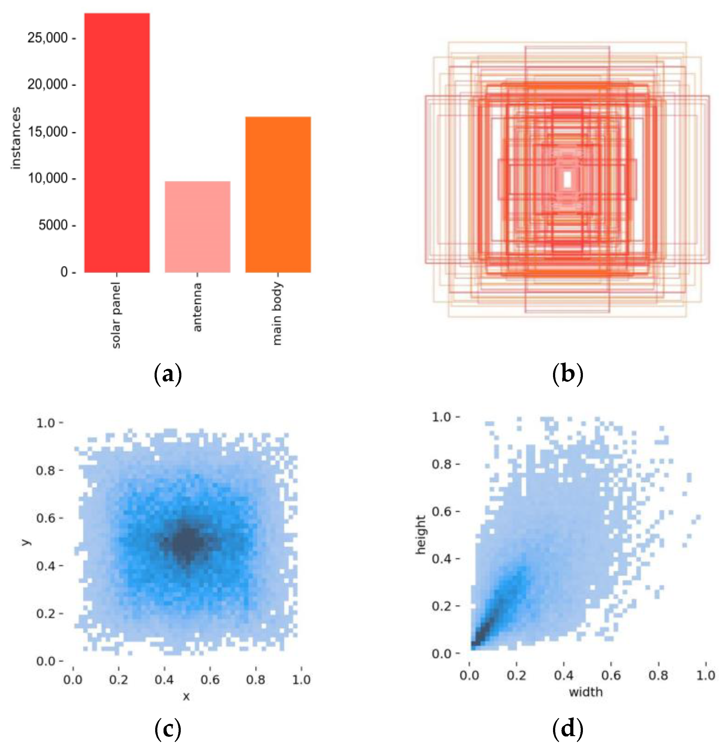
• A typical satellite component dataset was established, consisting of 3800 labeled satellite images. This is known to be the largest dataset of typical satellite components. By incorporating data augmentation techniques, the number of images in the dataset was expanded to 16,400, offering substantial support for future research in related fields.
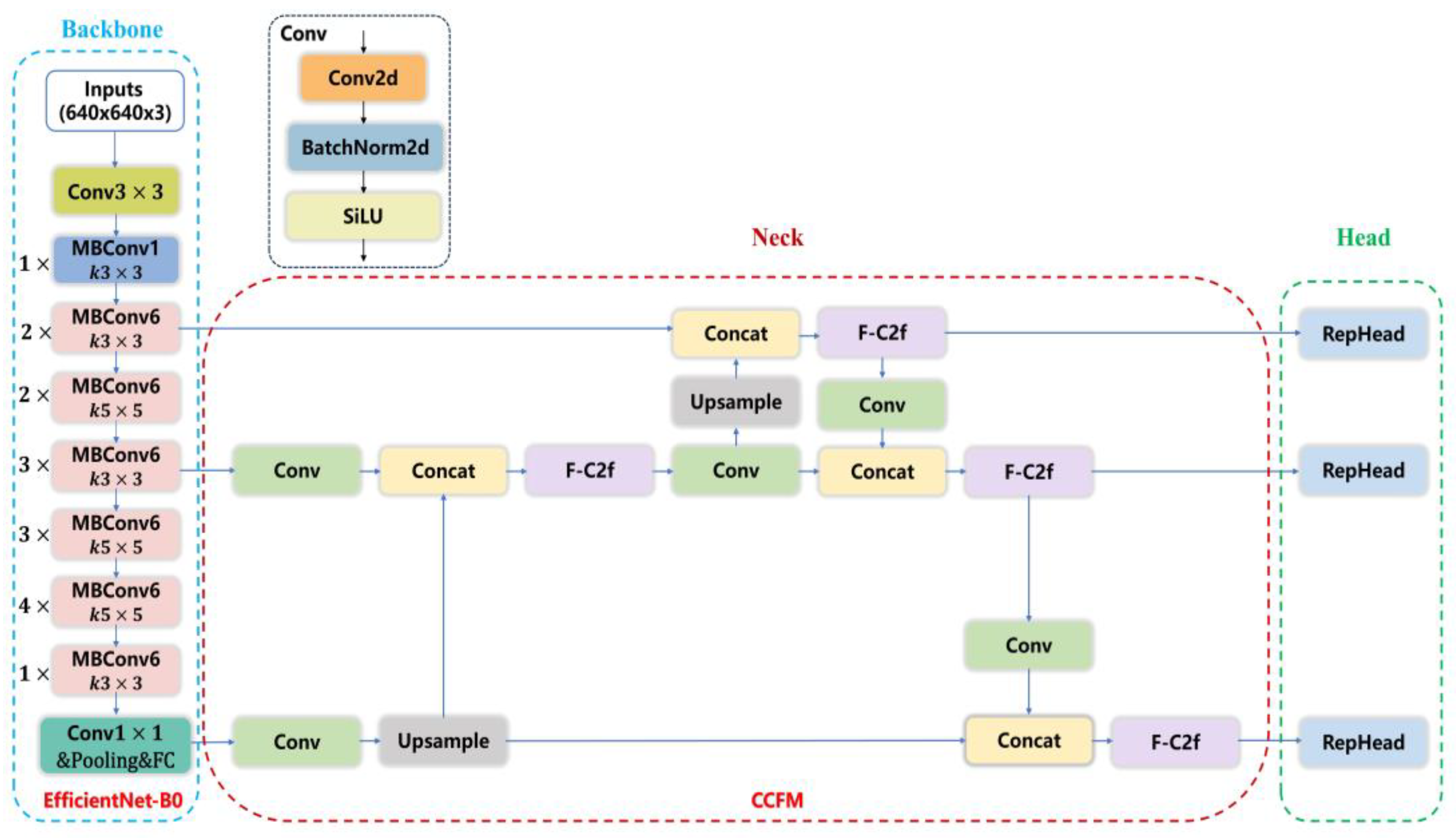
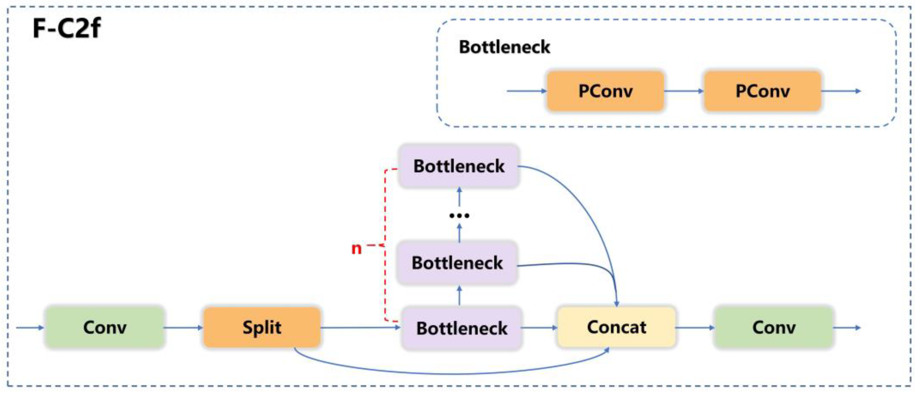
• To construct a lightweight detection model, this paper innovatively proposes the Faster-C2f (F-C2f) module and the RepHead detection head. The network structure is redesigned, utilizing the lightweight network EfficientNet-B0 as the Backbone of LTSCD-YOLO, and a lightweight Cross-Scale Feature Fusion Module was adopted in the Neck part. By fusing features of different resolutions across scales, the detection performance is enhanced.
• Focal-EIoU was adopted as the model’s loss function to obtain more accurate predicted bounding boxes, optimize the training process, and improve the model’s performance on typical satellite component detection tasks.

The following parts of the article are arranged as follows: Section 2 briefly introduces the YOLOv8 model and details the improvement strategies proposed in this paper. Section 3 describes the construction of the experimental dataset. Section 4 introduces the experimental details. Section 5 presents the backbone network comparison experiments, ablation experiments, comparative experiments with different models, visualization experiments, generalization experiments, and validation experiments. Section 6 is the discussion. Section 7 is the conclusions.

2. Methods

The YOLOv8 model, proposed by the Ultralytics team, consists of four main parts: Input, Backbone, Neck, and Head. (1) Input utilizes Mosaic data augmentation technology, which can provide the model with more training samples, enhancing the model’s performance and generalization capability. (2) Backbone adopts the Darknet53 structure, composed of 53 convolutional layers, including Conv modules, C2f (Faster Implementation of CSP Bottleneck with 2 convolutions) modules, and Spatial Pyramid Pooling Fast (SPPF) modules. (3) Neck utilizes a combination of Path Aggregation Network (PAN) and Feature Pyramid Network (FPN) [37], which can merge feature maps of different sizes, aiding in improving the model’s ability to detect targets of various scales. (4) Head adopts a decoupled head structure, separating classification from detection. Additionally, YOLOv8 transitions from an anchor-based to an anchor-free approach, reducing design complexity and enhancing model performance.

To meet the specific requirements for detecting typical components of satellites in space environments, this paper proposes LTSCD-YOLO, an improvement based on YOLOv8. The improved network structure is shown in Figure 2. (1) Input: It receives the original satellite images and processes them into a uniform size of $640\times 640\times 3$ (height $\times$ width $\times$ channels) for input into the network. (2) Backbone: Based on YOLOv8, the main network of the Backbone part is replaced with the lightweight network EfficientNet-B0.

Table 1. EfficientNet-B0 baseline network.

Stage $\mathit{i}$	Operator	Resolution ${\mathit{H}}_{\mathit{i}}\times {\mathit{W}}_{\mathit{i}}$	Channels ${\mathit{C}}_{\mathit{i}}$	Layers ${\mathit{L}}_{\mathit{i}}$
1	Conv$3\times 3$	$640\times 640$	32	1
2	MBConv1, k$3\times 3$	$320\times 320$	16	1
3	MBConv6, k$3\times 3$	$320\times 320$	24	2
4	MBConv6, k$5\times 5$	$160\times 160$	40	2
5	MBConv6, k$3\times 3$	$80\times 80$	80	3
6	MBConv6, k$5\times 5$	$40\times 40$	112	3
7	MBConv6, k$5\times 5$	$40\times 40$	192	4
8	MBConv6, k$3\times 3$	$20\times 20$	320	1
9	Conv$1\times 1$ & Pooling & FC	$20\times 20$	1280	1

Each row describes a stage $i$ with $L_i$ layers, with input resolution $H_i\times W_i$ and output channels $C_i$.

displays the network of EfficientNet-B0. (3) Neck: Uses a cross-scale fusion network structure to merge feature maps of different scales, enhancing the model’s adaptability to scale changes and its ability to detect small-scale objects. In addition, the C2f module in the Neck part is replaced with F-C2f (Faster-C2f) to further achieve model lightweighting. (4) Head: Uses RepHead based on RepConv [38] to enhance the model’s feature extraction capabilities. Finally, Focal-EIoU [39] is adopted as the loss function of the model to improve detection accuracy.

2.1. Lightweight Network Design

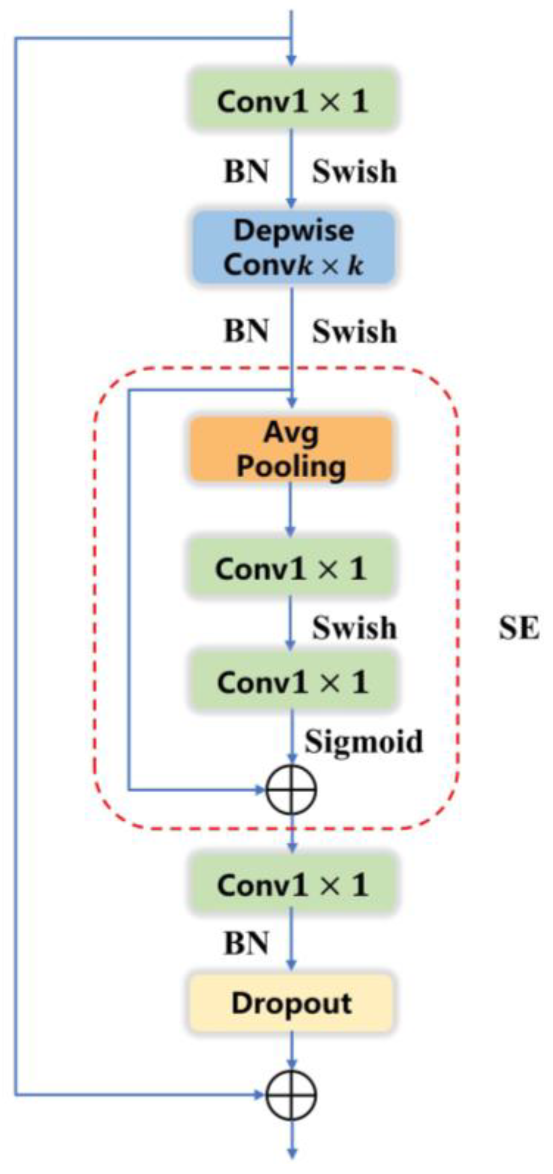
2.1.1. Backbone Network Improvement

To meet the detection task requirements in space environments, this paper chooses the relatively lightweight YOLOv8s as the baseline model after weighing detection accuracy and speed. EfficientNet-B0 [40] is used as the main backbone feature extraction network for LTSCD-YOLO. EfficientNet-B0 is a lightweight yet efficient convolutional neural network structure, mainly comprising three modules: the first module is a convolutional layer with a kernel size of $3\times 3$ and a stride of 2; the second module is the Mobile Inverted Bottleneck Convolution (MBConv) module; the third module consists of a convolutional layer with a kernel size of $1\times 1$, an average pooling layer, and a fully connected layer. Among them, the MBConv is the core module, where the number following MBConv (1 or 6) represents the channel expansion multiple for each module’s input feature matrix. The channel expansion multiple refers to how the number of channels in the input feature matrix is increased or kept the same through convolution operations in the neural network. Specifically, an expansion multiple of 1 means that the number of channels in the input feature matrix remains unchanged, while an expansion multiple of 6 means that the number of channels is expanded to 6 times the original, thereby enhancing the model’s capacity for representation. The $3\times 3$ or $5\times 5$ indicates the kernel size for the Depthwise Convolution. The structure of the MBConv is shown in Figure 3 and mainly includes: (1) $1\times 1$ convolution with an upscaling function; (2) $k\times k$ depthwise convolution; (3) the Squeeze-and-Excitation (SE) module; (4) $1\times 1$ convolution with a downscaling function; and (5) the Dropout layer. The $k\times k$ in the depthwise convolution corresponds to the $3\times 3$ and $5\times 5$ structures in EfficientNet-B0.

In the MBConv module, the input satellite image features first undergo a $1\times 1$ convolution with an upscaling function, followed by a $k\times k$ depthwise convolution to reduce computational load. Subsequently, an adaptive attention operation is performed through the squeeze-and-excitation module to obtain more effective image feature information, followed by a dimensionality reduction operation on the current features. Finally, a random dropout operation is executed through the dropout layer, enabling the model to learn more robust feature representations and enhancing the model’s generalization ability.

2.1.2. Neck Network Improvement

In this paper, the Neck adopts a Cross-Scale Feature-Fusion Module (CCFM) [41], which is an efficient deep learning structure designed to address scale variation issues in the field of computer vision. By fusing features of different scales, CCFM enhances the model’s adaptability to scale changes and its detection capability for small-scale objects. It can also effectively process details and global context information in images. This fusion strategy enables CCFM to demonstrate outstanding performance in a variety of visual tasks. The main advantages of CCFM include: (1) Multi-scale Feature Extraction Capabilities: CCFM integrates features from different levels of the network, addressing the issue of spatial detail loss due to the reduction in the size of feature maps as the network depth increases. This capability ensures that the model can capture complex semantic information while retaining rich spatial details, significantly improving the efficiency and capture ability of the model for features of various scales. (2) Adaptive Feature Fusion Capability: CCFM employs a strategy based on learned weights to automatically adjust the feature fusion approach. This grants the model a high degree of flexibility, allowing it to adapt the method of merging features from different layers according to the demands of different tasks, thereby enhancing the accuracy of the model in object detection tasks. (3) Excellent Performance with High Computational Efficiency: While improving model performance, CCFM also pays special attention to optimizing computational efficiency, ensuring that enhanced functionality does not come at the cost of computational resources. This design enables CCFM to perform high-precision processing of complex tasks in high-performance computing environments and supports operation on devices with limited computing resources, providing strong support for real-time or mobile applications.

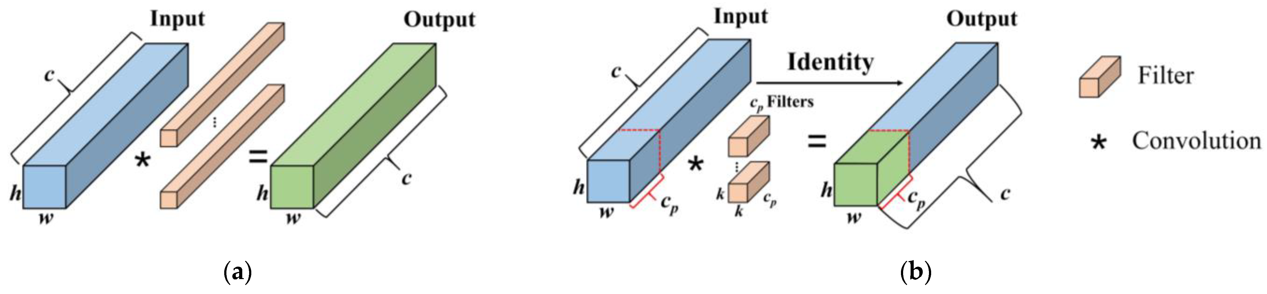
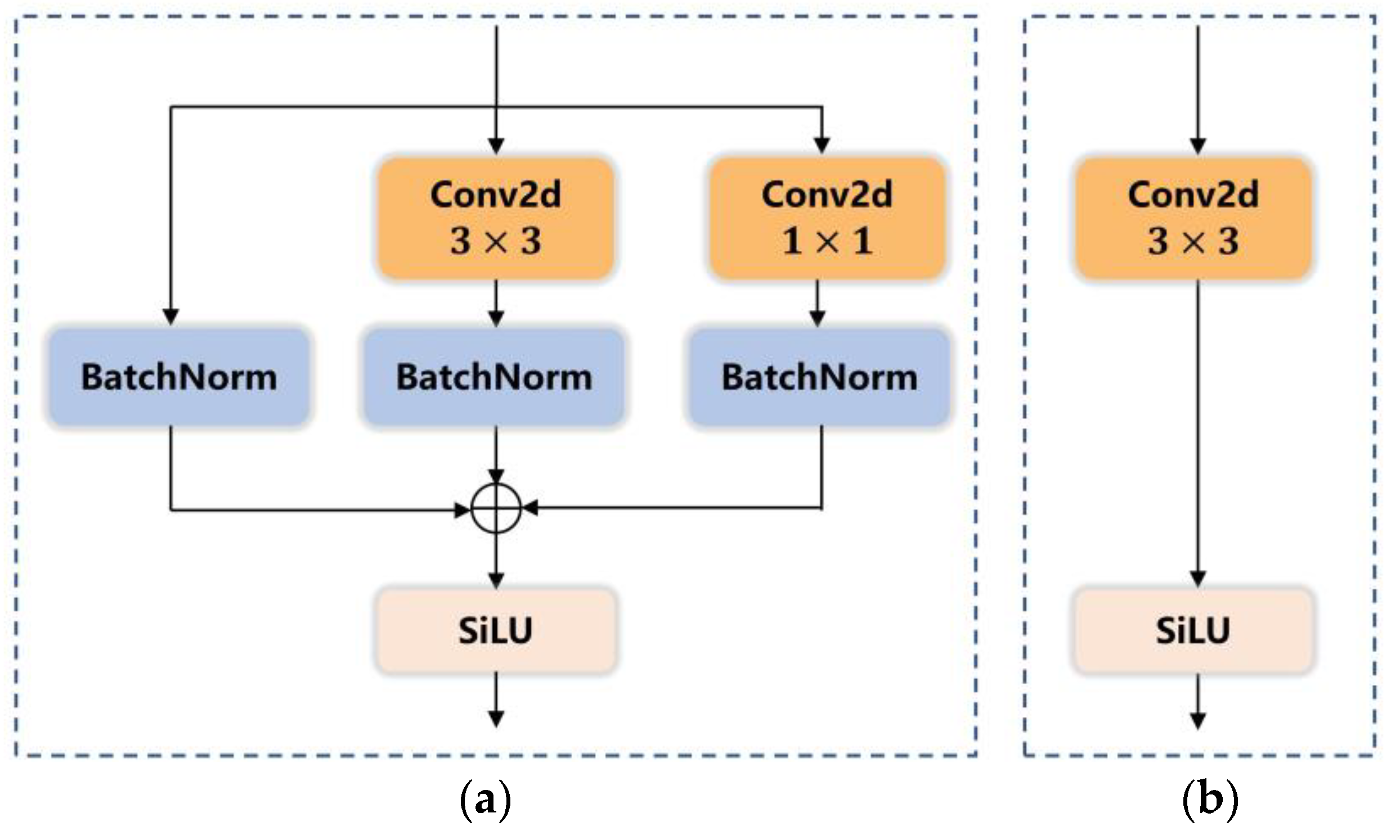
2.1.3. C2f Module Improvement

The YOLOv8 network architecture contains a large number of C2f modules, whose main function is feature extraction. The performance of the network is closely related to the feature learning of the C2f module. C2f modules typically employ conventional convolutions, leading to computational redundancy and increasing the model’s computational and parameter size. To address this issue, this paper designs a brand-new module based on the Partial Convolution (PConv) from FasterNet [42]—Faster-C2f (F-C2f) module, which simultaneously reduces computational redundancy and memory access. Figure 4b illustrates the working principle of PConv. It applies conventional convolution to only a part of the input channels for spatial feature extraction while keeping the remaining channels unchanged. For continuous or regular memory access, PConv considers the first or last $c_p$ continuous channels as a representative of the entire feature map for computation [42]. The input and output feature maps generally have the same number of channels, so the computational cost of PConv is:

$$h\times w\times k^2\times c_p^2$$

(1)

The memory access amount for PConv is:

$$h\times w\times 2c_p+k^2\times c_p^2\approx h\times w\times 2c_p$$

(2)

In this case, $h$ and $w$ represent the width and height of the feature map, respectively, $k$ represents the size of the convolutional kernel, c represents the number of input channels, and $c_p$ represents the number of channels involved in the convolution. Generally, it is often the case that $r=c_p/c=1/4$ (for example, selecting the first 25% of the channels); thus, the computational load of PConv is only $1/16$ of that of conventional convolution, and the number of memory accesses is only $1/4$ of that involved in conventional convolution operations.

The structural schematic of the F-C2f module is shown in Figure 5. Its main advantages include: (1) by adopting partial convolution technology, it achieves efficient feature extraction, significantly reducing the model’s computational complexity and memory access. (2) The F-C2f module inherits the multi-branch design of the C2f module, where the input data are split into two branches for processing. One branch is passed directly to the output, while the other branch is processed through n Bottleneck modules before being merged with the directly transmitted part. This design helps reduce redundant computations while enhancing the diversity of feature representations. Here, n represents the number of Bottleneck modules (default value is 1), and it can be adjusted based on specific requirements. Although each Bottleneck module has the same structure, the features extracted and processed by each module vary depending on their position in the network and the input they receive. For instance, the first Bottleneck module receives feature maps processed by the Conv layer, which are relatively close to the original features of the input image. Therefore, the first Bottleneck module processes more basic features. The subsequent Bottleneck modules receive the output from the previous Bottleneck module, and as each Bottleneck module further processes the input features, the later modules handle more complex and abstract feature information. Finally, these different levels of features are fused together to form an output feature map rich in information. This design significantly enhances the model’s ability to extract features, enabling the network to effectively capture various important details in the image. By maintaining a lightweight design, the F-C2f module successfully balances performance and speed, ensuring efficient operation of the model. (3) As a replacement for the C2f module, the F-C2f module can be seamlessly integrated into existing model architectures, allowing the model to be lightweight without needing major adjustments to the overall structure.

2.2. Optimize Loss Function

The bounding box regression loss function used by YOLOv8 is Complete Intersection over Union (CIoU) [43]. Its calculation formula is as follows:

$$CIoU=1-IoU+{\displaystyle \frac{{\rho }^2\left(b,b^{gt}\right)}{c^2}}+\alpha v$$

(3)

$$\alpha ={\displaystyle \frac{v}{\left(1-IoU\right)+v}}$$

(4)

$$v={\displaystyle \frac{4}{{\pi }^2}}{(arctan{\displaystyle \frac{w^{gt}}{h^{gt}}}-arctan{\displaystyle \frac{w}{h}})}^2$$

(5)

$$\begin{gathered} {\displaystyle \frac{\partial v}{\partial w}}={\displaystyle \frac{8}{{\pi }^2}}(arctan{\displaystyle \frac{w^{gt}}{h^{gt}}}-arctan{\displaystyle \frac{w}{h}})\times {\displaystyle \frac{h}{w^2+h^2}} \\ {\displaystyle \frac{\partial v}{\partial h}}=-{\displaystyle \frac{8}{{\pi }^2}}(arctan{\displaystyle \frac{w^{gt}}{h^{gt}}}-arctan{\displaystyle \frac{w}{h}})\times {\displaystyle \frac{h}{w^2+h^2}} \end{gathered}$$

(6)

In the formula, $b$ and $b^{gt}$ represent the center points of the predicted box and true box, respectively; $\rho (·)$ denotes the Euclidean distance between the two points; $IoU$ represents the Intersection over Union ($IoU$) between the predicted box and the true box. $c$ is the diagonal length of the smallest enclosing box covering both the predicted and true boxes. $\alpha$ and $v$ are hyperparameters. $w$ and $h$ represent the width and height of the predicted box, respectively, and $w^{gt}$ and $h^{gt}$ represent the width and height of the true box, respectively.

Equations (3)–(6) constitute the complete expression for the CIoU loss function. Although the CIoU loss function takes into account multiple geometric features of the predicted and true boxes, including aspect ratio, center distance, and overlap area, to improve the accuracy of regression localization, CIoU still has the following shortcomings: (1) When $\left\{\left(\left.w=k{w}^{gt},h=k{h}^{gt}\right|k\in R^{+}\right)\right\}$ occurs, it can cause $v=0$, and the loss function is unable to make an effective judgment at this time; (2) as can be seen from Equation (6), ${\displaystyle \frac{\partial v}{\partial w}}$ and ${\displaystyle \frac{\partial v}{\partial h}}$ have opposite signs, which means that the aspect ratio of the anchor boxes cannot increase or decrease simultaneously, leading to the predicted boxes not fitting the true boxes well; (3) using the aspect ratio alone cannot effectively reflect the discrepancy between the anchor boxes and the true boxes, and there are some limitations in dealing with small annotated boxes and non-overlapping low-quality annotated boxes during regression.

To address the above issues and enhance the model’s performance, this paper adopts Focal-EIoU as a replacement for CIoU. The calculation formula for Focal-EIoU is as follows:

$$L_{EIoU}=1-IoU+{\displaystyle \frac{{\rho }^2\left(b,b^{gt}\right)}{c_w^2+c_h^2}}+{\displaystyle \frac{{\rho }^2\left(w,w^{gt}\right)}{c_w^2}}+{\displaystyle \frac{{\rho }^2\left(h,h^{gt}\right)}{c_h^2}}$$

(7)

$$L_{f(x)}=\left\{\begin{array}{c}-{\displaystyle \frac{\alpha x^2[2\mathit{ln}\left(\beta x\right)-1]}{4}},0<x\le 1;{\displaystyle \frac{1}{e}}\le \beta \le 1\\ -\alpha \mathit{ln}\left(\beta \right)x+C,x>1;{\displaystyle \frac{1}{e}}\le \beta \le 1\end{array}\right.$$

(8)

$$L_{Focal-EIoU}={IoU}^{\gamma }{L}_{EIoU}$$

(9)

In the formula: $c_w$ and $c_h$ indicate the width and height of the smallest enclosing area for both the predicted and true boxes; $x$ represents the difference between the true values and predicted values; $e$ is the natural constant; $\beta$ is used to control the curvature of the curve; $C$ is a constant; and $\gamma$ is a parameter used to control the degree of outlier suppression.

Efficient Intersection over Union (EIoU) improves upon the shortcomings of CIoU by dividing the loss function into three parts: distance loss, aspect ratio loss, and IoU loss. It modifies the aspect ratio component in CIoU to address issues arising from the use of aspect ratios.

Due to the complexity of space environments, the quality of images is highly susceptible to disturbances from surrounding environmental factors, leading to fluctuations in image quality. Especially when images contain a lot of noise and have indistinct contours, deep learning models are prone to false negatives and false positives. This results in an imbalance between foreground and background content, making it easy to generate a large number of easily distinguishable candidate boxes and negative examples during training. This imbalance causes the model to perform well in recognizing easy samples but poorly in handling hard-to-identify samples. Therefore, to improve model performance, FocalL1 loss is used to set different gradients, as shown in Equation (8), applying higher gradients to areas with higher error rates. This approach focuses more on the recognition of difficult samples, reducing the impact of low-quality samples on model performance. By combining EIoU loss with FocalL1 loss, the final Focal-EIoU loss is obtained. Equation (9) presents the complete expression for Focal-EIoU loss. This loss function not only better adapts to the needs of space scenes but also enhances the model’s target recognition accuracy and robustness.

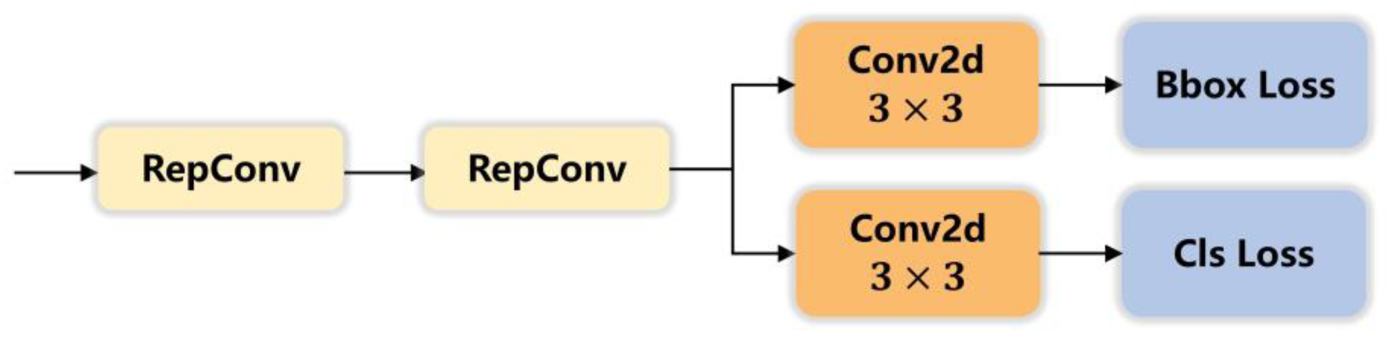
2.3. Detection Head Improvement

The detection head of YOLOv8 adopts a decoupled head structure, consisting of two branches: one for calculating classification loss and the other for calculating anchor box loss. Each branch contains two convolutional blocks. To enhance the feature fusion and feature extraction capabilities of the model’s detection head, enabling it to better handle difficult samples in complex environments without significantly increasing computational burden, this paper proposes a novel detection head structure called RepHead. The core idea of RepHead is to utilize the re-parameterization capability of RepConv, which is a basic component of the RepVGG network. RepConv employs a convolution re-parameterization method. During the training phase, RepConv uses a parallel structure of BatchNorm, $1\times 1$ convolution, and $3\times 3$ convolution to enrich multi-scale information. In the validation phase, the convolution re-parameterization method merges multiple branches into a single branch structure, and the re-parameterization module achieves efficient and high-precision detection through a $3\times 3$ convolution. RepConv uses multi-branch convolution layers during the training phase and re-parameterizes the parameters of branches onto the main branch during the validation phase, thus reducing computation and memory consumption. The RepConv structure is shown in Figure 6.

The structure of RepHead is shown in Figure 7. This design significantly reduces the model’s parameter count and computational load while maintaining high accuracy.

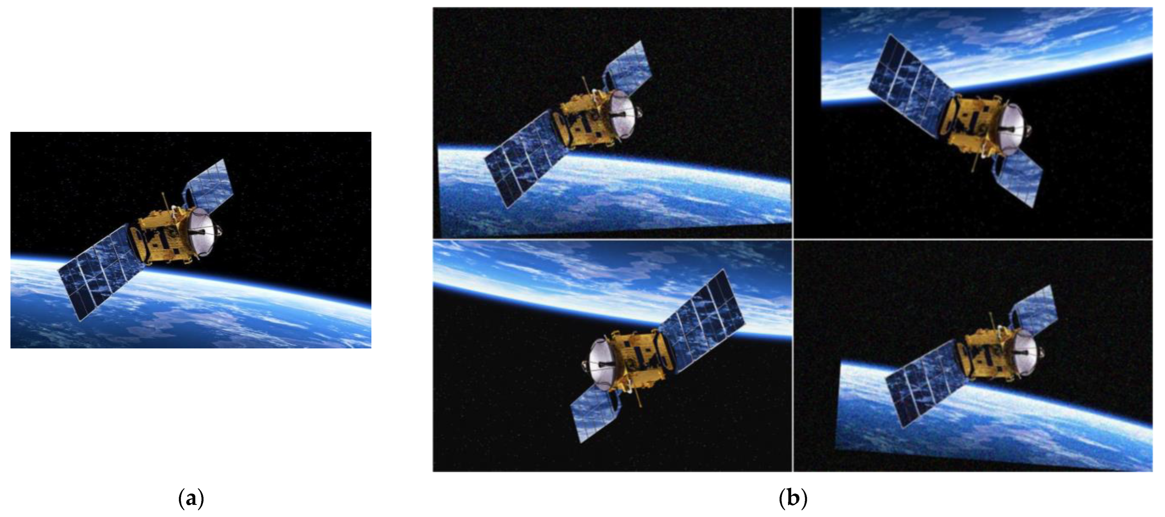
3. Construction of the Experimental Dataset

The success of deep learning models often requires a large amount of training data to achieve good performance. However, the number of spatial datasets available for training deep learning models is currently very limited, especially in the field of satellite imagery. This is because satellite images are often considered sensitive data, and genuine satellite image resources are scarce. To address this issue, we have created the TSC-Dataset, which aims to provide more available resources for the field of remote sensing. This will enable researchers to develop and test new algorithms more effectively, especially in achieving breakthroughs in the recognition of typical satellite components. This contribution is of great significance for advancing the development and application of remote sensing technology.

The TSC-Dataset is sourced from four main parts: (1) 2351 valid satellite images filtered from the Satellite-Dataset [44]; (2) 976 satellite images of 92 satellites were collected from various perspectives and orbital positions using the STK 11.6 (Satellite Tool Kit 11.6) software; (3) 273 satellite images obtained through web scraping; (4) 200 real satellite images gathered from organizations such as NASA, the ESA, and the NSSDC. Some of these images are shown in Figure 8.

In the process of collecting satellite images using STK software, to minimize the differences between simulated images and real-scene images as much as possible, this paper considered the specific locations of satellites and the lighting environment around them. By sampling satellites at high, medium, and low orbital positions, different imaging effects were obtained, thereby better simulating real scenes.

Figure 9 shows a comparison between the real image and the simulated image of the Artemis satellite. In this comparison, the various components of the Artemis satellite are very similar in terms of outline, shape, color, and texture, with the only difference being in brightness. It can be seen that the simulated image reasonably replicates the details and characteristics of the real image.

The final dataset includes 3800 satellite images, comprising real images, simulated images, and synthetic images, with a diverse range of satellite types to ensure dataset diversity. These images were annotated at the pixel level using labelimg 1.8.6 software. This paper categorizes the satellites into three typical parts, namely the solar panel, the main body, and the antenna (as shown in Figure 10). The annotation results are directly saved as XML files to facilitate the unification of the dataset into the PASCAL VOC format. This paper will use 200 real satellite images collected from institutions such as NASA for the final testing experiments to verify the generalization capability of the model. The remaining 3600 images will be used for training and evaluating the model. These images will be divided into training, validation, and test sets in a ratio of 7:2:1, resulting in 2520 images for the training set, 720 images for the validation set, and 360 images for the test set.

The TSC-Dataset covers various types of satellite components, including the antenna, the solar panel, and the main body. These components come from different types of satellites, such as communication satellites, Earth observation satellites, and navigation satellites. As shown in Figure 11, these satellites have similar visual characteristics. For example, the outlines of the solar panels are mostly rectangular, with colors primarily in blue or black. The outlines of the antennas are mostly circular, and their fronts are usually white. The outlines and colors of these local components change with the satellite’s attitude and orbital position.

The imaging characteristics of space objects include variability of viewing angles, blurriness of images, and uneven brightness, among others. To simulate real imaging conditions in the space environment, improve the model’s generalization and robustness, and enhance the model’s diversity and adaptability, this paper employs data augmentation techniques to expand the training set. The specific augmentation operations include:

Rotation: Each image has a 50% probability of being rotated, with the rotation angle randomly selected between −10° and 10°. This simulates variations in satellite images caused by observations from different angles.

Translation: Each image has a 30% probability of being translated horizontally or vertically. The translation distance is determined as a certain proportion of the image size, simulating displacement errors during the imaging process.

Mirroring: Each image has a 40% probability of being mirrored horizontally or vertically, further increasing the diversity of perspectives.

Color Adjustment and Scaling: Color adjustments include modifying brightness and saturation, while scaling involves changing the image size. Both transformations have a probability of 45%, adapting to different lighting conditions and resolution changes.

Noise Addition and Brightness Adjustment: Given the common occurrence of uneven brightness and noise in space environments, these two augmentation operations are set with a probability of 70%. The noise added is Gaussian noise; for brightness adjustment, a random value $alpha$ between 0.35 and 1.25 is set to determine the brightness level during the data augmentation process. A lower $alpha$ value darkens the image, while a higher value brightens it.

Each data augmentation transformation depends on an independent random probability. Therefore, an image can undergo multiple operations such as rotation, translation, and noise addition in one data augmentation process, significantly increasing the diversity of the data. This helps in training a more robust model. The number of data augmentations for each image in the training set is set to 5. After data augmentation, the training set expands from 2520 images to 15,120 images. The number of images in the validation and test sets remains unchanged, resulting in a total of 16,400 satellite images. The augmented images are shown in Figure 12.

To intuitively and conveniently display the distribution characteristics of different types and sizes of typical satellite components in the dataset, we conducted a detailed statistical analysis of the annotation files of the TSC-Dataset. The analysis results are shown in Figure 13, which includes four parts: Figure 13a presents a histogram of the distribution of the number of categories in the training set, from which one can intuitively understand the quantity situation of each type of component; Figure 13b visually shows the distribution of the length and width of all annotation boxes by setting the center points $x$, $y$ coordinates of all annotation boxes at the same position, helping to observe the characteristics of size distribution; Figure 13c is a histogram of the $x$, $y$ coordinates used to analyze the distribution of annotation box center points in the image; and Figure 13d shows the histogram of the width and height variables of the annotation boxes.

4. Experimental Detail

4.1. Experimental Environment

The experimental environment configuration is shown in

Table 2. Configuration of the experimental environment.

Experimental Environment	Details
Operating system	Ubuntu18.04
GPU	NVIDIA GeForce RTX 3090, 24 GB
CPU	Intel Xeon Gold 6248R
Memory	125 G
Programming language	Python3.8.18
Framework	PyTorch 1.11.0 + CUDA 11.3 + cuDNN 8.2.0
IDE	PyCharm2022.3.3

.

The training parameters are set as follows: the training period is 300 epochs, the batch is set to 32, and the image size is set to $640\times 640$. The model uses the SGD optimizer for parameter optimization, with an initial learning rate set at $1\times {10}^{-2}$ and a momentum parameter set at 0.937. To prevent overfitting, the model employs a weight decay strategy, with the weight decay value set at $5\times {10}^{-4}$.

4.2. Experimental Evaluation Criteria

To accurately analyze the model’s detection performance on typical satellite components in a space environment, we selected Precision ($P$), Recall ($R$), Mean Average Precision ($mAP$), model parameter count ($Params$), model computation load ($GFLOPs$), and frames per second ($FPS$) as evaluation metrics to assess the overall performance of the model.

Precision ($P$) is an indicator measured based on the prediction results, representing the proportion of actual positive cases among all samples predicted as positive. In the prediction results, samples deemed positive can be divided into two categories: True Positive ($TP$) and False Positive ($FP$). A prediction is considered positive if the sample’s $IoU$ is greater than or equal to a specific confidence threshold; otherwise, if the $IoU$ is less than this threshold, the prediction is deemed negative. Precision can be represented by Equation (10).

$$Precision={\displaystyle \frac{TP}{TP+FP}}$$

(10)

Recall ($R$) is an assessment metric of the model’s comprehensiveness in detection, indicating the proportion of samples correctly predicted as positive among all actual positive samples. The definition of correctly predicted as positive is $TP$, and the definition of wrongly predicted as negative is $FN$. Recall is represented by Equation (11).

$$Recall={\displaystyle \frac{TP}{TP+FN}}$$

(11)

By taking precision as the vertical axis and recall as the horizontal axis, the model’s performance $P-R$ curve can be obtained. The area under the $P-R$ curve is the Average Precision ($AP$) for single-class labels, represented by Equation (12).

$$AP={\int }_0^{1}P(R)dR$$

(12)

For detection targets of $N$ categories, the mean of average precision across categories is represented by Equation (13). All $AP$ that are averaged in the given equation were computed for the IoU threshold of 0.5.

$$mAP={\displaystyle \frac{{\sum }_{n=1}^N{AP}_n}{N}}$$

(13)

$mAP$ is one of the most important model performance evaluation metrics in the field of object detection, used to measure the model’s detection accuracy and comprehensiveness across multiple categories.

In real-world object detection scenarios, in addition to pursuing high accuracy, the model’s detection speed is also very important. The model’s detection speed is commonly measured by $FPS$ (frames per second), which is the number of images the model can process per second.

The model parameter count ($Params$) refers to the total number of all parameters during the model training process. This parameter count reflects the model’s spatial complexity and overall scale, thereby becoming a key indicator to measure the model’s lightweight level.

The model computation load ($GFLOPs$) refers to the number of floating-point operations required for the model to perform one forward propagation process. It is an indicator to evaluate the model’s consumption of computational resources.

5. Results

To verify the effectiveness and advancement of the LTSCD-YOLO algorithm in detecting typical satellite components, we designed six sets of experiments. These include a backbone network comparison experiment, an ablation experiment, a comparative experiment with different models, visualization experiments, a generalization experiment, and a validation experiment. The aim is to comprehensively evaluate the performance of the proposed algorithm in detecting typical satellite components.

5.1. Backbone Network Comparison Experiment

To select a suitable model for detecting typical satellite components in space scenes, this paper improves upon the backbone part of YOLOv8 by replacing it with some of the current mainstream feature extraction networks. The results of the backbone network comparison experiment on the test set are shown in

Table 3. Backbone network comparison experiment results.

	Backbone Network	P/%	R/%	mAP@0.50/%	Params/106	GFLOPs/G	FPS/(frame·s−1)
	CSPDarknet (Baseline)	92.9	88.2	93.1	11.14	28.8	98.04
	RepViT-M0_9 [45]	92.0	85.6	92.0	8.57	22.7	80.64
Vision	EfficientViT_M0 [46]	91.0	83.6	90.0	8.38	20.4	56.75
Transformers	EfficientViT_M1 [46]	93.0	83.9	91.0	9.03	25.1	57.69
	MobileViTv1-XXS [47]	92.4	86.3	92.2	7.64	20.9	76.92
	MobileViTv2-XXS [48]	92.9	86.7	92.6	7.71	22.4	81.56
	Mobilenetv3_small [49]	90.1	84.8	89.7	6.73	16.7	90.91
	ShuffleNetv2 [50]	91.4	83.5	89.3	5.94	16.0	105.65
ConvNets	VanillaNet-5 [51]	91.4	80.6	88.5	6.36	18.3	117.65
	FasterNet [42]	89.3	85.2	90.2	6.08	16.1	114.94
	GhostNetV2 [52]	92.9	86.0	92.0	8.24	19.1	75.56
ConvNets	Efficientnet_B0	93.5	87.5	92.8	6.53	17.3	96.15

.

The backbone network, as the foundational part of the model, directly influences the overall model’s performance and resource consumption, making it crucial for achieving model lightweighting. In selecting the backbone network, this paper considers multiple factors, including the model’s parameter size, computational load, and performance metrics. As seen from Table 3, this paper compares the performance of various advanced convolutional neural networks and Vision Transformer architectures in the task of recognizing typical satellite components. Compared to the Vision Transformer architectures in the table, EfficientNet_B0 achieved the best performance (precision: 93.5, recall: 87.5, mAP50: 92.8) with the smallest parameter count and computation load. Despite the Vision Transformers’ excellent performance in many computer vision tasks, their substantial computational requirements and slow detection speed make them less suitable for use in resource-constrained space environments. Compared to the convolutional neural networks in the table, EfficientNet_B0 also achieved the best performance (precision: 93.5, recall: 87.5, mAP50: 92.8) with relatively smaller parameter count and computation load. Compared to the baseline model, when EfficientNet_B0 was used as the backbone network, the parameter count decreased by 41.38%, the computational load decreased by 39.93%, and the precision increased by 0.65%. Despite the significant reductions in parameter count and computation load, EfficientNet_B0 still achieved high detection speed and accuracy. The results indicate that EfficientNet_B0, while maintaining high accuracy, demonstrates significant advantages in model size and computational efficiency, making it an ideal choice in resource-constrained environments.

5.2. Ablation Experiment

To verify the effect of different improvement modules on model performance, we designed an ablation experiment. By gradually introducing different improvement modules, we assessed the impact of each module on model performance. These improvement modules include replacing the backbone part with the EfficientNet_B0 feature extraction network, improving the Neck to a CCFM structure, improving the C2f module to an F-C2f, replacing the original loss function with Focal-EIoU, and adopting a RepHead detection head. In the ablation experiment, these improvement modules were introduced one by one to observe changes in model performance and explore the contribution of each improvement module to model performance, providing guidance and reference for model optimization. The results are shown in

Table 4. Results of the ablation experiment.

Group	A1	A2	A3	A4	A5	mAP@0.50/%	Params/106	GFLOPs/G	FPS/(frame·s−1)
1	—	—	—	—	—	93.1	11.14	28.8	98.04
2	√	—	—	—	—	92.8	6.53	17.3	96.15
3	—	√	—	—	—	93.2	7.26	23.2	107.53
4	—	—	√	—	—	93.8	7.59	19.7	104.17
5	—	—	—	√	—	94.3	11.14	28.8	119.05
6	—	—	—	—	√	93.5	15.82	32.9	98.75
7	—	√	—	—	√	93.7	7.05	21.9	103.09
8	√	√	—	—	—	93.0	2.90	12.3	103.74
9	√	√	√	—	—	93.4	2.63	11.0	108.15
10	√	√	√	√	—	94.0	2.63	11.0	113.35
11	√	√	√	√	√	94.5	2.40	9.8	115.35

A1 represents EfficientNet_B0; A2 represents CCFM; A3 represents F-C2f; A4 represents Focal-EIoU; A5 represents RepHead. Group 1 is the baseline model using CSPDarknet, without any modifications.

.

From the ablation study results in Table 4, it can be seen that after replacing the original model’s backbone network with EfficientNet_B0, the model’s mAP50 and detection speed slightly decreased, but the parameter count and computational load were reduced by 41.38% and 39.93%, respectively. This demonstrates the effectiveness of the improved module in achieving a lightweight model. After improving the Neck part to a CCFM structure, the model’s parameter count was reduced by 34.83%, the computational load was reduced by 19.44%, the detection speed increased by 9.68%, and the mAP50 improved by 0.11%. The overall performance of the model was significantly enhanced, demonstrating the effectiveness of the CCFM structure. After improving the original model’s C2f module to the F-C2f module with PConv, the model’s parameter count decreased by 31.87%, the computational load decreased by 31.59%, the detection speed increased by 6.25%, and the mAP50 improved by 0.75%. The overall performance of the model was significantly enhanced, demonstrating the effectiveness of the F-C2f module. When the loss function of the original model was replaced with Focal-EIoU, mAP50 increased by 1.29%, and detection speed improved by 21.43%, while maintaining the same number of parameters and computational load. This indicates that Focal-EIoU can effectively enhance the model’s detection accuracy and speed. When the RepHead module is added to the original model, although the number of parameters and computational load increase, both the mAP50 and detection speed improve. Notably, when the CCFM module and RepHead module are added together to the original model, the model’s parameter count and computational load decrease more compared to adding the CCFM module alone, and both the mAP50 and detection speed are significantly improved. This result indicates that the combination of the CCFM and RepHead modules can more effectively optimize the model’s performance. When EfficientNet_B0 and CCFM are applied to the original model simultaneously, the model’s parameter count is reduced by 73.97%, and computational load is reduced by 57.29%, the detection speed is improved by 5.81%, and the mAP50 only decreases by 0.11%. This significantly reduces the model’s parameters and computational load while maintaining high accuracy. Based on the original model, after simultaneously adding EfficientNet_B0, CCFM, and F-C2f modules and improving the loss function to Focal EIoU, the model significantly reduced the number of parameters and computational load while maintaining high accuracy. At the same time, the detection speed was notably enhanced, achieving comprehensive improvements. With all improvement modules integrated, compared to the original model, the mAP50 increased to 94.5% (an increase of 1.50%), the parameter count decreased by 78.46%, the computational load decreased by 65.97%, and the detection speed increased by 17.66%, achieving a relatively ideal improvement effect.

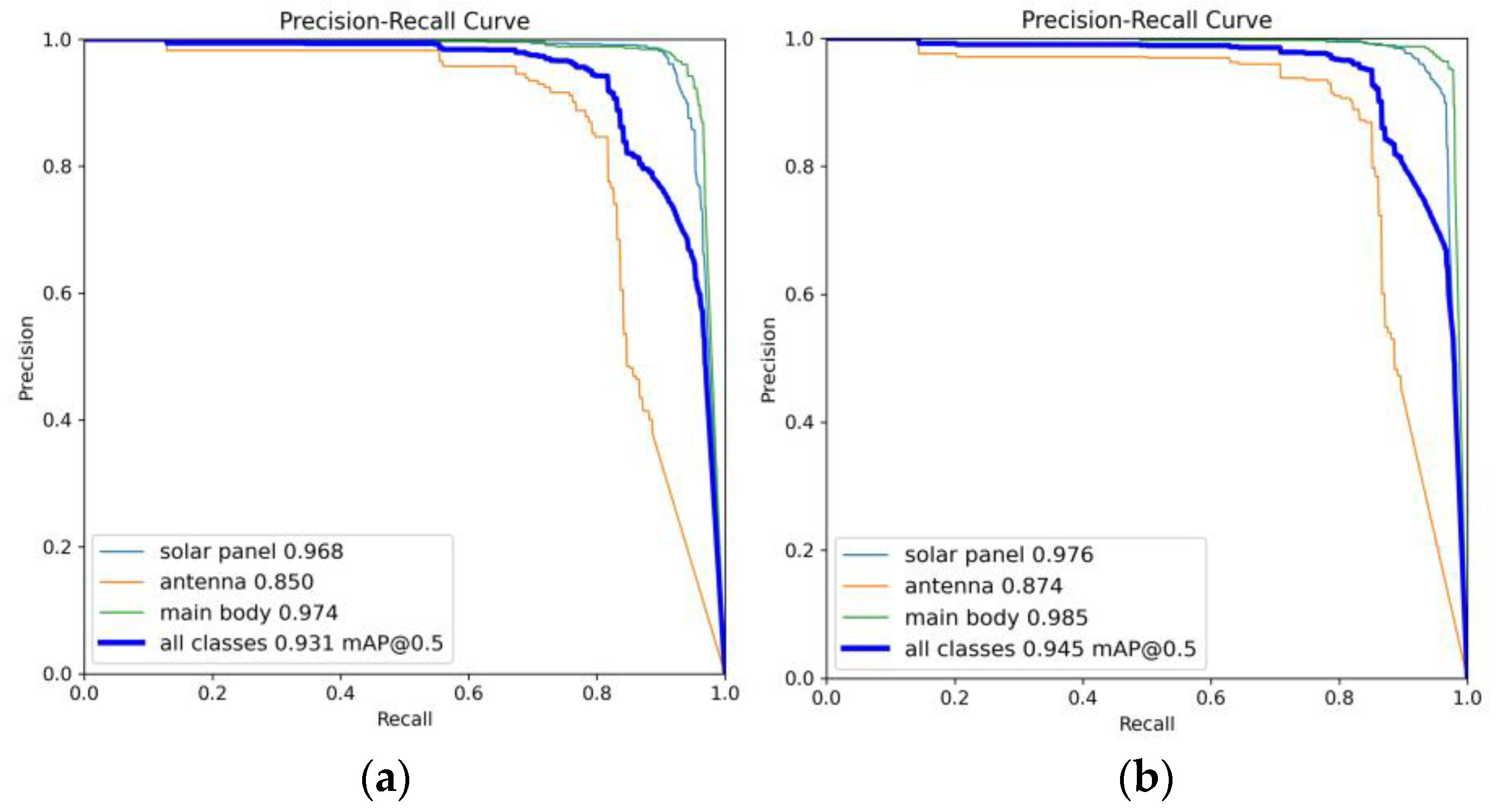
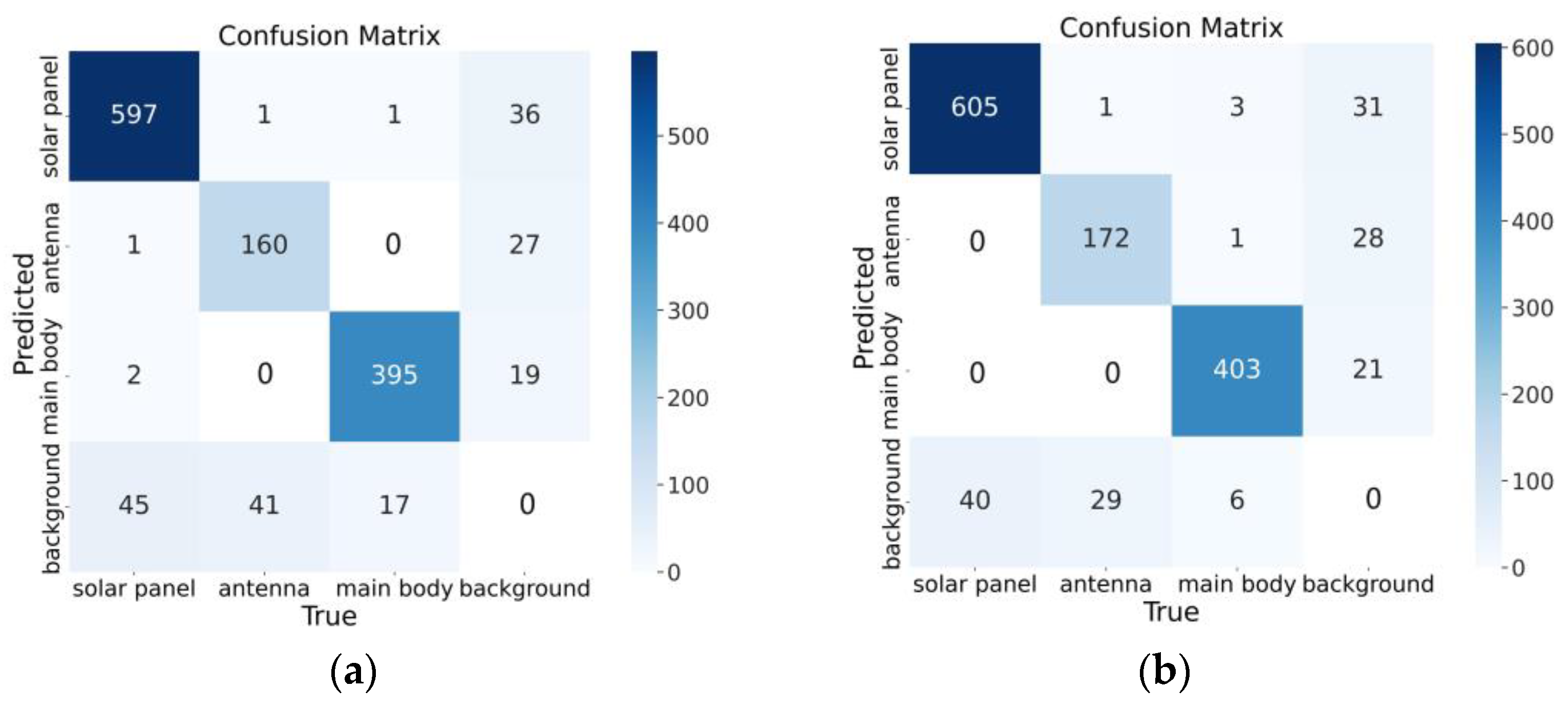
5.3. Comparative Experiment of Different Models

To further verify the effectiveness of LTSCD-YOLO, we conducted comparative experiments with other mainstream object detection algorithms, including the original models and improved models of the YOLO series as well as the DETR model, such as YOLOv3-tiny, YOLOv4-CSP, YOLOv5s, YOLOv6n, YOLOv7-tiny, YOLOv7, YOLOv8s, YOLOv8s-ghost, YOLOV9t, YOLOv9s, YOLOv10s, and DETR [41]. The results are shown in

Table 5. Comparative experimental results of different models.

Model	P/%	R/%	mAP@0.50/%	Params/106	GFLOPs/G	FPS/(frame·s−1)
YOLOv3-tiny	88.7	83.3	88.7	12.13	18.9	143.85
YOLOv4-CSP	89.4	84.2	89.7	52.50	119.7	72.15
YOLOv5s	93.8	86.8	92.4	7.03	16.0	86.2
YOLOv6n	89.2	81.1	88.9	4.5	11.8	90.09
YOLOv7-tiny	94.2	85.8	92.0	6.02	13.2	85.29
YOLOv7	94.6	89.4	93.8	36.49	103.2	74.86
YOLOv8s	92.9	88.2	93.1	11.14	28.8	98.04
YOLOv8s-ghost	93.6	87.0	91.9	5.92	16.1	90.91
YOLOv9t	92.1	88.4	92.9	2.62	10.7	50.36
YOLOv9s	95.0	89.9	94.3	9.60	38.7	41.67
YOLOv10s	93.4	87.9	93.3	8.04	24.5	97.59
RT-DETR-ResNet50	92.4	87.2	92.3	42.0	130.5	22.69
RT-DETR-ResNet101	93.0	88.3	93.2	61.76	191.4	16.89
DETR-L	92.3	87.2	92.2	32.8	108.0	25.35
DETR-X	92.4	89.2	93.5	67.3	232.3	15.68
Ours	95.7	88.2	94.5	2.40	9.8	115.35

.

According to the data in Table 5, compared with the YOLO series and the DETR series, the LTSCD-YOLO algorithm proposed in this paper achieves the highest precision (95.7%) and mAP50 (94.5%) with the smallest parameter and computational load, and has the second fastest detection speed. Although YOLOv3-tiny has the fastest detection speed, its precision, recall rate, and mAP50 are respectively 7.31%, 5.56%, and 6.14% lower than those of LTSCD-YOLO, and it has a larger parameter and computational load, making its overall performance inferior to LTSCD-YOLO. Although YOLOv9s achieves the highest recall rate of 89.9%, its detection speed is slower, and both the parameter count and computational load are much higher compared to LTSCD-YOLO, resulting in overall performance that is inferior to LTSCD-YOLO. Compared to LTSCD-YOLO, the DETR series has a much larger parameter count and computational load and slower detection speed, making it unsuitable for deployment in resource-limited space environments. The results indicate that LTSCD-YOLO surpasses the other algorithms in the table in overall performance, especially due to its small parameter count and computational load, high precision, and fast detection speed, making it highly suitable for detection tasks in space environments.

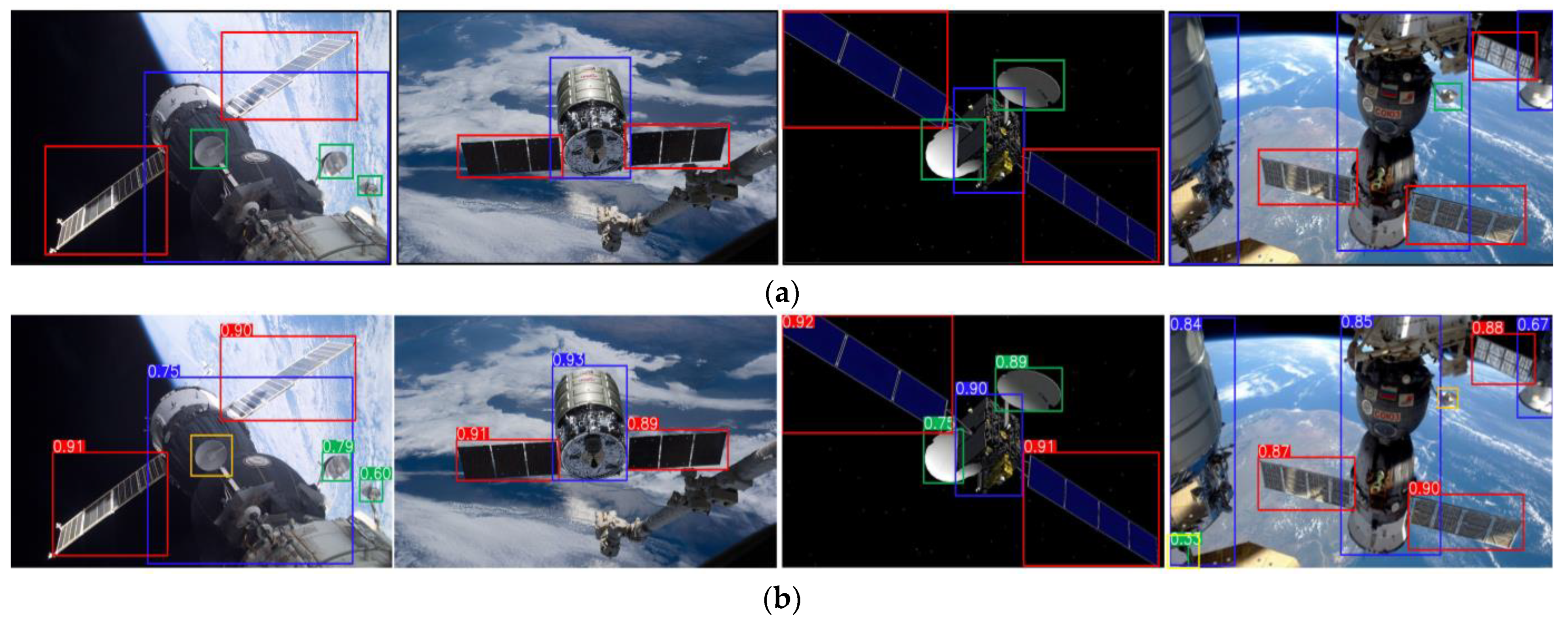
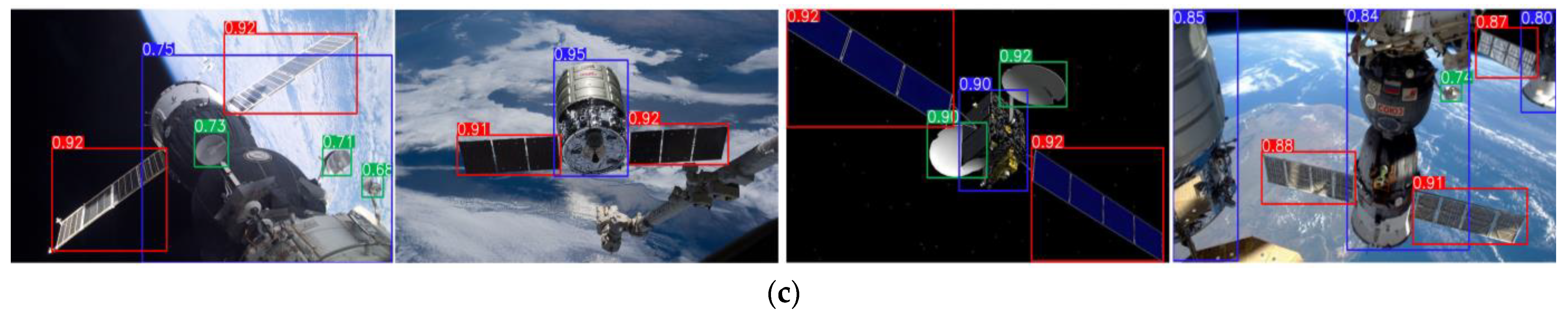
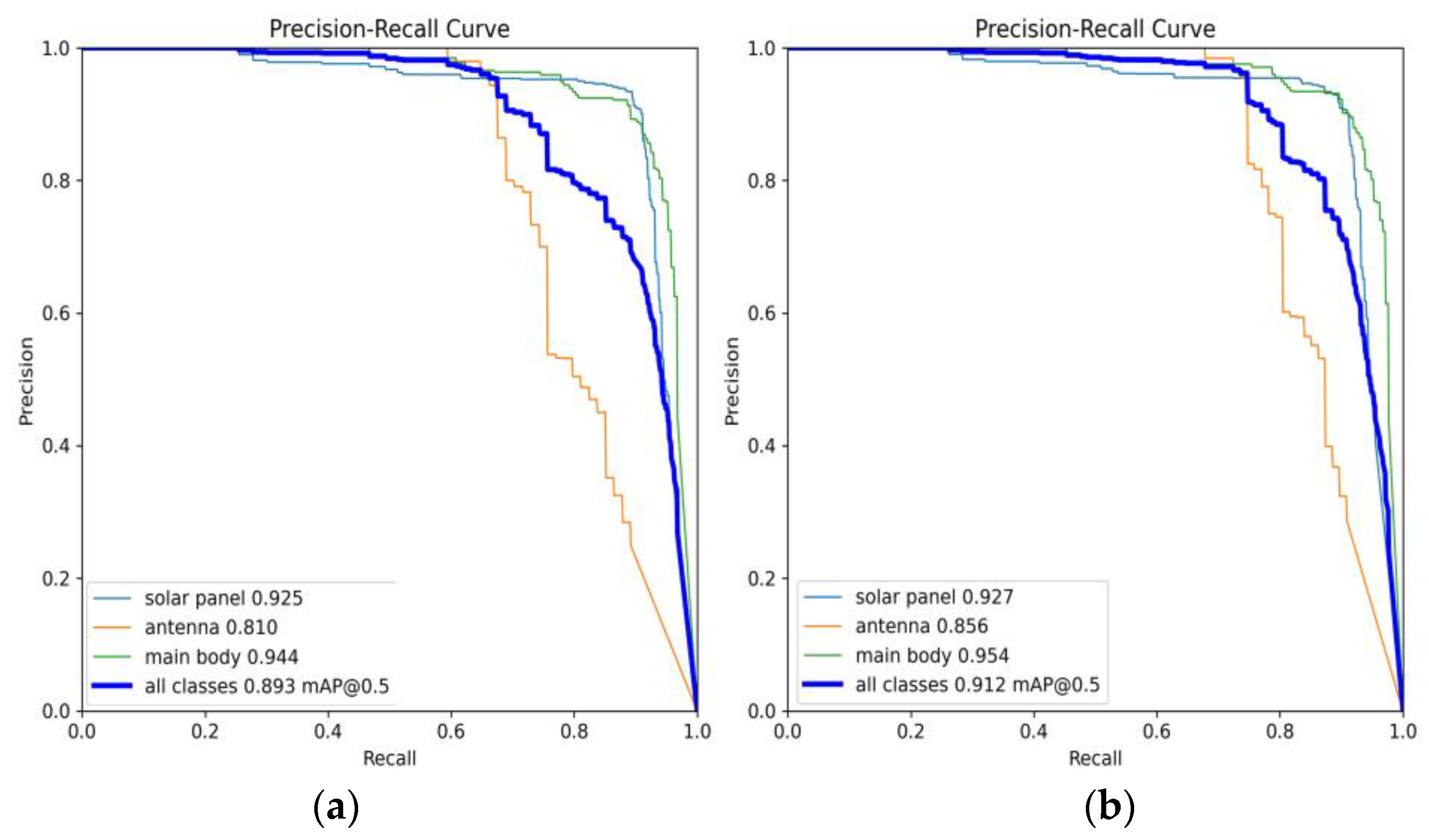
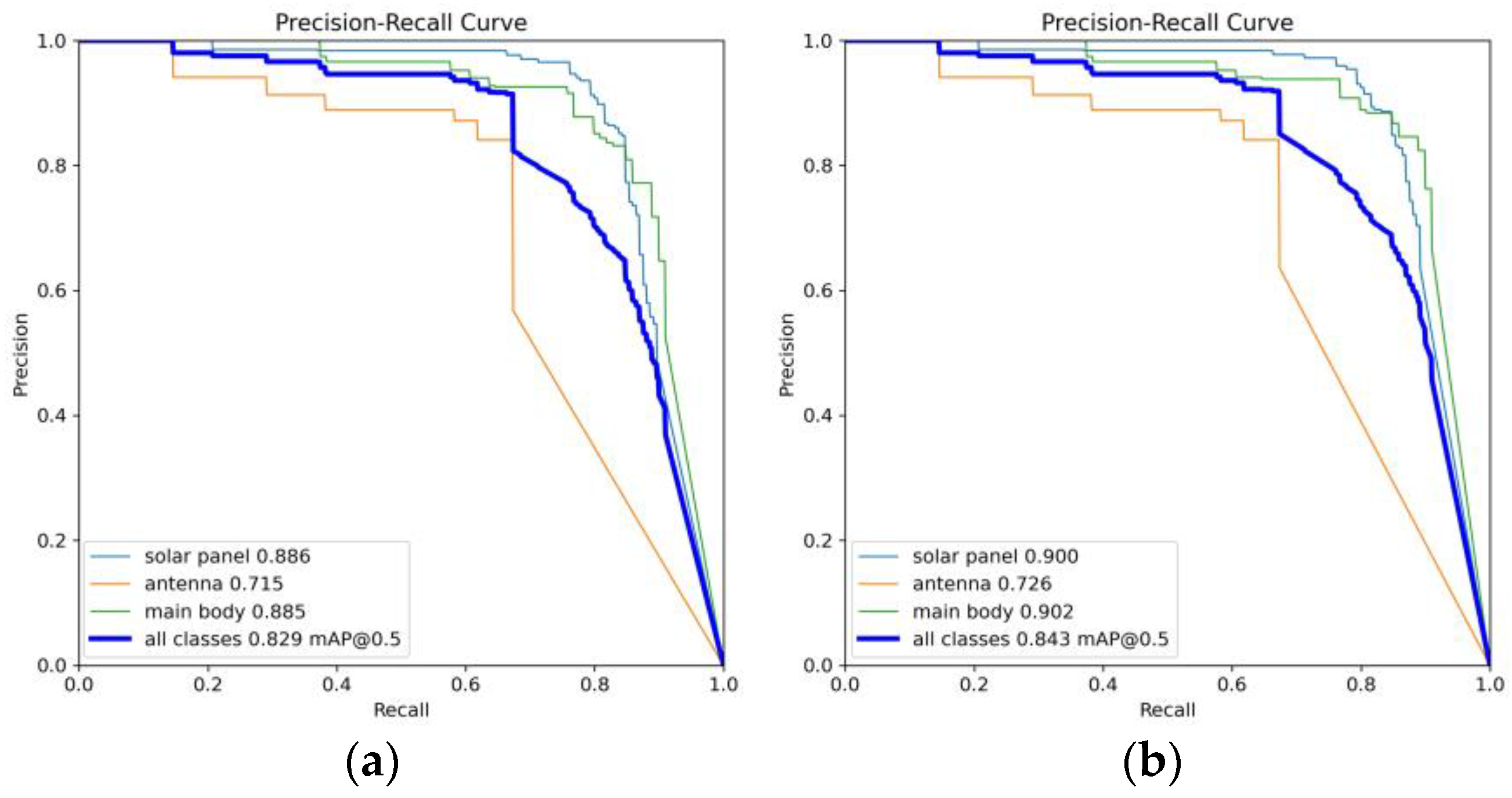
5.4. Visualization Experiments

In the visualization experiments, the performance and accuracy of the two models, YOLOv8s and LTSCD-YOLO, can be intuitively compared through their P-R curves. The detection results of YOLOv8s are shown in Figure 14a, while those of LTSCD-YOLO are displayed in Figure 14b. From these figures, it’s observable that LTSCD-YOLO achieves an mAP50 of 97.6% for solar panel detection, which is an 0.83% increase compared to YOLOv8s; an mAP50 of 87.4% for antenna detection, a 2.82% increase; and an mAP50 of 98.5% for main body detection, a 1.13% increase.

A confusion matrix is a tool used to evaluate model performance. It reflects the relationship between the model’s prediction and the actual situation of sample data, thereby assessing the model’s classification performance. In a confusion matrix, the horizontal axis represents the actual labels, and the vertical axis represents the predicted labels. Elements on the diagonal indicate perfect agreement between predictions and actual outcomes, while other elements show the number of samples misclassified. Ideally, the confusion matrix would be a diagonal matrix, indicating outstanding classification ability. Figure 15a shows the confusion matrix obtained from training YOLOv8s, and Figure 15b shows the one from LTSCD-YOLO. The comparison of confusion matrices shows that the LTSCD-YOLO model performs better in reducing missed and false detections. The relationship between actual and predicted values in the LTSCD-YOLO model’s confusion matrix closely follows the characteristics of a diagonal matrix, thereby proving the model’s superior performance.

To investigate the model’s detection performance on different typical satellite components, we selected 360 satellite images for testing. From

Table 6. Comparison of detection performance for solar panel, antenna, and main body.

Model	Typical Satellite Components	P/%	R/%	Params/106	GFLOPs/G	Number of Images
YOLOv8 (Baseline)	Solar panel	95.8	91.9	11.14	28.8	360
	Antenna	86.9	78.9
	Main body	96.0	93.7
LTSCD-YOLO (Ours)	Solar panel	96.0	93.1	2.40	9.8	360
	Antenna	88.8	83.2
	Main body	96.4	96.8

, it can be seen that the precision rate of LTSCD-YOLO in solar panel detection is 96.0%, an increase of 0.21% compared to YOLOv8s; the recall rate is 93.1%, an increase of 1.31% compared to YOLOv8s. In antenna detection, the precision rate is 88.8%, an increase of 2.19% compared to YOLOv8s; the recall rate is 83.2%, an increase of 5.45% compared to YOLOv8s. In main body detection, the precision rate is 96.4%, an increase of 0.42% compared to YOLOv8s; the recall rate is 96.8%, an increase of 3.31% compared to YOLOv8s. It can be seen that LTSCD-YOLO, while significantly reducing the number of model parameters and the computational load, achieves a comprehensive improvement in the detection precision and recall rates for solar panels, antenna, and the main body, with the most notable improvement in recall rates.

For a straightforward and intuitive depiction of the detection effect of the proposed LTSCD-YOLO model, different satellite images were selected for visualization experiments, providing a direct comparison between YOLOv8s and LTSCD-YOLO, with some results shown in Figure 16. Figure 16a represents the Ground Truth, Figure 16b represents the YOLOv8s detection results, and Figure 16c represents the LTSCD-YOLO detection results, where red boxes detect solar panels, green boxes detect antennas, blue boxes detect the main body, yellow boxes represent false detections, and orange boxes represent missed detections. The results indicate that YOLOv8s had one false detection and two missed detections, while LTSCD-YOLO did not have issues with false or missed detections and also demonstrated improved detection accuracy, further proving the effectiveness of the improved LTSCD-YOLO model and its reliable support for typical satellite component detection tasks.

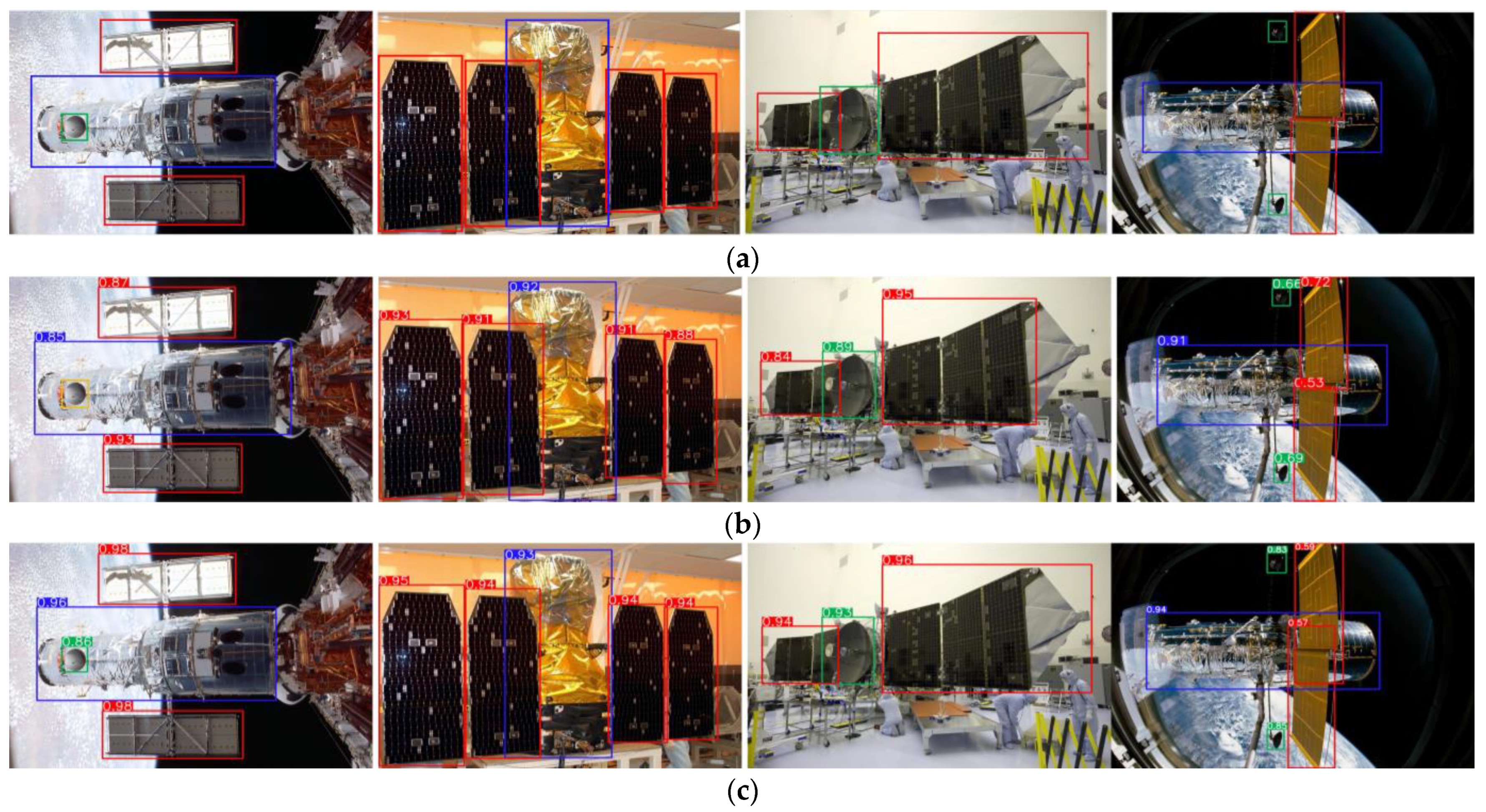
5.5. Generalization Experiment

To further verify the model’s generalization, we finally chose to conduct experiments on 200 real satellite images that came from various institutions including NASA, and had never been used during the model’s training or validation phases. By carrying out testing on these new datasets, we can more accurately assess the model’s efficiency and stability when handling unknown data. The results of the experiment will help us understand the reliability of the model in real-world applications, thereby providing guidance for further optimization and application of the model. Moreover, this will also demonstrate the model’s adaptability in diverse environments and verify whether its performance remains consistent under various conditions.

The P-R curves allow for a visual comparison of the performance and accuracy of the YOLOv8s and LTSCD-YOLO models on real satellite images. The detection results of YOLOv8s are shown in Figure 17a, while the detection results of LTSCD-YOLO are shown in Figure 17b. From these figures, it can be seen that the overall mAP50 of LTSCD-YOLO is 91.2%, which is 2.13% higher than YOLOv8s. In solar panel detection, LTSCD-YOLO achieved a mAP50 of 92.7%, 0.22% higher than YOLOv8s; a mAP50 of 85.6% in antenna detection, 5.68% higher; and a mAP50 of 95.4% in main body detection, 1.06% higher.

Figure 18 visually demonstrates the detection performance of the LTSCD-YOLO and YOLOv8s models on real satellite images. Figure 18a represents the Ground Truth, Figure 18b represents the detection results of YOLOv8s, and Figure 18c represents the detection results of LTSCD-YOLO. The results indicate that YOLOv8s had one missed detection, while LTSCD-YOLO had no issues with missed detections and demonstrated higher detection accuracy. This further proves the effectiveness of the improved LTSCD-YOLO model in detecting real satellite images and its generalization ability.

5.6. Validation Experiment

To strengthen the validation of the method proposed in this paper, we constructed a small dataset consisting of real satellite images. This dataset contains 500 satellite images. Due to the limited number of training samples, the features that the model can learn are also limited, which is both a challenge and a test for the model’s performance. We divided the dataset into training, validation, and test sets in a 6:2:2 ratio, resulting in 300 images for training, 100 images for validation, and 100 images for testing. We performed data augmentation on the training set, expanding it to 1800 images, while keeping the validation and test sets unchanged, ultimately obtaining 2000 real satellite images.

The detection results of YOLOv8s are shown in Figure 19a, and the detection results of LTSCD-YOLO are shown in Figure 19b. As can be seen from these figures, in this small real satellite image dataset, the overall mAP50 of LTSCD-YOLO is 84.3%, which is 1.69% higher than YOLOv8s. In solar panel detection, LTSCD-YOLO achieved an mAP50 of 90.0%, 1.58% higher than YOLOv8s; in antenna detection, LTSCD-YOLO achieved an mAP50 of 72.6%, 1.54% higher; and in main body detection, LTSCD-YOLO achieved an mAP50 of 90.2%, 1.92% higher. From the test results, it can be seen that the proposed model performs well on the small real satellite image dataset, further proving the effectiveness of the model proposed in this paper.

6. Discussion

6.1. Memory Application Analysis of the LTSCD-YOLO Algorithm

To further explore the application environment of the LTSCD-YOLO algorithm, the paper investigated the memory sizes of different types of satellites. Small satellites typically have memory spaces ranging from a few hundred MB to several tens of GB, such as CubeSats (Cube Satellites) [53], which are commonly used for low-cost scientific missions, educational projects, and technology validation, with each satellite having memory sizes of up to 16 GB. Medium satellites have memory spaces ranging from several hundred GB to several TB, such as Landsat 8 [54], which is used for Earth resource monitoring, environmental management, and disaster response, capturing multispectral images for geographic information analysis. Large satellites have memory spaces ranging from several TB to tens of TB, such as GOES-16 (Geostationary Operational Environmental Satellite) [55], used for monitoring and predicting weather and environmental changes. Currently, space-grade NAND flash [56] technology supports storage capacities ranging from 32 GB to 256 GB, with read and write speeds of about 100 megabytes per second. Additionally, flash memory chips have been specially designed for radiation resistance to operate long-term in harsh space environments. The next generation of earth observation satellites will have onboard storage capacities of several TB to handle the collected remote sensing data. The optimal weight file size of LTSCD-YOLO is 5.1 MB, and it requires about 2 GB of memory to operate, making it suitable for use on small satellites like CubeSats for typical satellite component detection tasks.

6.2. Limitations and Future Work

The experimental results show that the proposed model has broad application prospects. In scenarios involving the identification of cooperative satellites, since the configurations of the satellites are usually known, using these known satellites to train the model can achieve better recognition results in practical applications. Additionally, the model is also applicable to identifying non-cooperative target satellites. In such cases, since the satellite configurations are unknown, the model must rely on features learned from other satellites to identify these unknown satellites. According to the experiments presented in this paper, the model also performs excellently in these scenarios. However, the current model can detect only a limited variety of satellite components and is unable to identify specific satellite names. Future research can focus on further exploring how to determine the specific names of satellites based on their features and identify more satellite components.

In this paper, although the LTSCD-YOLO model demonstrates significant advantages in detecting typical satellite components, it still has some limitations. Firstly, the TSC-Dataset used in this paper contains a limited number of real satellite images. To improve the training effectiveness and adaptability of the model, future research should include more real satellite images. Secondly, although the proposed model performs well in terms of parameter count, detection speed, and accuracy, there is still room for improvement. With the continuous updates and optimizations of the YOLO model, future research can reduce the number of model parameters and improve detection speed and accuracy based on the updated YOLO models to better meet the demands of the space environment. Finally, considering the complexity and harshness of the space environment, future research can incorporate more transformations in data augmentation to obtain features that are closer to the space environment, thereby further optimizing model training and achieving better results. It is hoped that through further optimization, better performance can be achieved in the detection of typical satellite components in the future.

7. Conclusions

To address the limitations of storage space and computational resources in space environments, this paper proposes a lightweight satellite component detection algorithm called LTSCD-YOLO. The backbone network of this algorithm is based on EfficientNet_B0; it introduces a cross-scale feature fusion module in the Neck part and upgrades the C2f module to the F-C2f module. The Head part employs RepHead, and the loss function uses Focal-EIoU. By adopting an efficient network structure design and advanced model optimization techniques, this algorithm significantly reduces the number of model parameters and computational load while ensuring the reliability and accuracy of detection performance. To further enhance the model’s training effectiveness, we systematically collected, organized, precisely annotated, and preprocessed a large amount of satellite imagery data to construct a comprehensive and diverse Typical Satellite Components Dataset (TSC-Dataset). The dataset was expanded to 16,400 images using data augmentation techniques, providing strong support for future research in this field. Experimental results on the TSC-Dataset show that, compared to YOLOv8s, LTSCD-YOLO improves the mean Average Precision (mAP50) by 1.50%, reduces the number of model parameters by 78.46%, decreases computational load by 65.97%, and increases detection speed by 17.66%. The algorithm’s generalization was also verified on real satellite images. These results demonstrate that the LTSCD-YOLO model can quickly and accurately identify satellite components, validating the effectiveness of the algorithm.

The above results indicate that LTSCD-YOLO can provide reliable technical support for satellite component detection tasks. It has broad application prospects in the field of remote sensing and is expected to promote further development in this area.

References

1. Satellite Database|Union of Concerned Scientists. Available online: https://www.ucsusa.org/resources/satellite-database (accessed on 26 June 2024).
2. Zhang, H.; Zhang, C.; Jiang, Z.; Yao, Y.; Meng, G. Vision-Based Satellite Recognition and Pose Estimation Using Gaussian Process Regression. Int. J. Aerosp. Eng. 2019, 2019, 5921246. [Google Scholar] [CrossRef]
3. Volpe, R.; Circi, C. Optical-Aided, Autonomous and Optimal Space Rendezvous with a Non-Cooperative Target. Acta Astronaut. 2019, 157, 528–540. [Google Scholar] [CrossRef]
4. Liu, L.; Zhao, G.; Bo, Y. Point Cloud Based Relative Pose Estimation of a Satellite in Close Range. Sensors 2016, 16, 824. [Google Scholar] [CrossRef]
5. Opromolla, R.; Fasano, G.; Rufino, G.; Grassi, M. A Review of Cooperative and Uncooperative Spacecraft Pose Determination Techniques for Close-Proximity Operations. Prog. Aerosp. Sci. 2017, 93, 53–72. [Google Scholar] [CrossRef]
6. Cao, S.; Mu, J.; Wu, H.; Liang, Y.; Wang, G.; Wang, Z. Recognition and Instance Segmentation of Space Non-Cooperative Satellite Components Based on Deep Learning. In Proceedings of the 2021 China Automation Congress (CAC), Kunming, China, 22–24 October 2021; pp. 7734–7739. [Google Scholar]
7. Leung, S.; Montenbruck, O. Real-Time Navigation of Formation-Flying Spacecraft Using Global-Positioning-System Measurements. J. Guid. Control Dyn. 2005, 28, 226–235. [Google Scholar] [CrossRef]
8. Massimi, F.; Ferrara, P.; Petrucci, R.; Benedetto, F. Deep Learning-Based Space Debris Detection for Space Situational Awareness: A Feasibility Study Applied to the Radar Processing. IET Radar Sonar Navig. 2024, 18, 635–648. [Google Scholar] [CrossRef]
9. Cai, J.; Huang, P.; Chen, L.; Zhang, B. A Fast Detection Method of Arbitrary Triangles for Tethered Space Robot. In Proceedings of the 2015 IEEE International Conference on Robotics and Biomimetics (ROBIO), Zhuhai, China, 6–9 December 2015; IEEE: Piscataway, NJ, USA, 2015; pp. 120–125. [Google Scholar]
10. Du, X.; Liang, B.; Xu, W.; Qiu, Y. Pose Measurement of Large Non-Cooperative Satellite Based on Collaborative Cameras. Acta Astronaut. 2011, 68, 2047–2065. [Google Scholar] [CrossRef]
11. Peng, J.; Xu, W.; Yan, L.; Pan, E.; Liang, B.; Wu, A.-G. A Pose Measurement Method of a Space Noncooperative Target Based on Maximum Outer Contour Recognition. IEEE Trans. Aerosp. Electron. Syst. 2020, 56, 512–526. [Google Scholar] [CrossRef]
12. Girshick, R.; Donahue, J.; Darrell, T.; Malik, J. Rich Feature Hierarchies for Accurate Object Detection and Semantic Segmentation. In Proceedings of the IEEE/CVF Conference on Computer Vision and Pattern Recognition, Columbus, OH, USA, 23–28 June 2014; pp. 580–587. [Google Scholar]
13. He, K.; Zhang, X.; Ren, S.; Sun, J. Spatial Pyramid Pooling in Deep Convolutional Networks for Visual Recognition. IEEE Trans. Pattern Anal. Mach. Intell. 2015, 37, 1904–1916. [Google Scholar] [CrossRef] [PubMed]
14. Girshick, R. Fast R-CNN. In Proceedings of the IEEE International Conference on Computer Vision (ICCV), Santiago, Chile, 7–13 December 2015; pp. 1440–1448. [Google Scholar]
15. Ren, S.; He, K.; Girshick, R.; Sun, J. Faster R-CNN: Towards Real-Time Object Detection with Region Proposal Networks. IEEE Trans. Pattern Anal. Mach. Intell. 2016, 39, 1137–1149. [Google Scholar] [CrossRef] [PubMed]
16. He, K.; Gkioxari, G.; Dollár, P.; Girshick, R. Mask R-CNN. In Proceedings of the IEEE International Conference on Computer Vision (ICCV), Venice, Italy, 22–29 October 2017; pp. 2961–2969. [Google Scholar]
17. Redmon, J.; Divvala, S.; Girshick, R.; Farhadi, A. You Only Look Once: Unified, Real-Time Object Detection. In Proceedings of the IEEE Conference on Computer Vision and Pattern Recognition, Las Vegas, NV, USA, 27–30 June 2016; IEEE: Piscataway, NJ, USA, 2016; pp. 779–788. [Google Scholar]
18. Redmon, J.; Farhadi, A. YOLO9000: Better, Faster, Stronger. In Proceedings of the IEEE Conference on Computer Vision and Pattern Recognition, Honolulu, HI, USA, 21–26 July 2017; pp. 7263–7271. [Google Scholar]
19. Redmon, J.; Farhadi, A. YOLOv3: An Incremental Improvement. arXiv 2018, arXiv:1804.02767. [Google Scholar]
20. Bochkovskiy, A.; Wang, C.-Y.; Liao, H.-Y.M. YOLOv4: Optimal Speed and Accuracy of Object Detection. arXiv 2020, arXiv:2004.10934. [Google Scholar]
21. Jocher, G. YOLOv5 [EB/OL]. Available online: https://github.com/ultralytics/yolov5 (accessed on 14 April 2024).
22. Li, C.; Li, L.; Jiang, H.; Weng, K.; Geng, Y.; Li, L.; Ke, Z.; Li, Q.; Cheng, M.; Nie, W.; et al. YOLOv6: A Single-Stage Object Detection Framework for Industrial Applications. arXiv 2022, arXiv:2209.02976. [Google Scholar]
23. Wang, C.-Y.; Bochkovskiy, A.; Liao, H.-Y.M. YOLOv7: Trainable Bag-of-Freebies Sets New State-of-the-Art for Real-Time Object Detectors. In Proceedings of the IEEE/CVF Conference on Computer Vision and Pattern Recognition, Vancouver, BC, Canada, 17–24 July 2023; pp. 7464–7475. [Google Scholar]
24. Jocher, G. YOLOv8 [EB/OL]. Available online: https://github.com/ultralytics/ultralytics (accessed on 14 April 2024).
25. Wang, C.-Y.; Yeh, I.-H.; Liao, H.-Y.M. YOLOv9: Learning What You Want to Learn Using Programmable Gradient Information. arXiv 2024, arXiv:2402.13616. [Google Scholar]
26. Wang, A.; Chen, H.; Liu, L.; Chen, K.; Lin, Z.; Han, J.; Ding, G. YOLOv10: Real-Time End-to-End Object Detection. arXiv 2024, arXiv:2405.14458. [Google Scholar]
27. Cao, J.; Bao, W.; Shang, H.; Yuan, M.; Cheng, Q. GCL-YOLO: A GhostConv-Based Lightweight YOLO Network for UAV Small Object Detection. Remote Sens. 2023, 15, 4932. [Google Scholar] [CrossRef]
28. Chen, G.; Cheng, R.; Lin, X.; Jiao, W.; Bai, D.; Lin, H. LMDFS: A Lightweight Model for Detecting Forest Fire Smoke in UAV Images Based on YOLOv7. Remote Sens. 2023, 15, 3790. [Google Scholar] [CrossRef]
29. Liu, Y.; Ma, Y.; Chen, F.; Shang, E.; Yao, W.; Zhang, S.; Yang, J. YOLOv7oSAR: A Lightweight High-Precision Ship Detection Model for SAR Images Based on the YOLOv7 Algorithm. Remote Sens. 2024, 16, 913. [Google Scholar] [CrossRef]
30. Zeng, H.; Xia, Y. Space Target Recognition Based on Deep Learning. In Proceedings of the 2017 20th International Conference on Information Fusion (Fusion), Xi’an, China, 10–13 July 2017; IEEE: Piscataway, NJ, USA, 2017; pp. 1–5. [Google Scholar]
31. Fomin, I.S.; Bakhshiev, A.V.; Gromoshinskii, D.A. Study of Using Deep Learning Nets for Mark Detection in Space Docking Control Images. Procedia Comput. Sci. 2017, 103, 59–66. [Google Scholar] [CrossRef]
32. Wang, L.; Xiao, H.; Bai, C. Spatial Multi-Object Recognition Based on Deep Learning. In Proceedings of the 2019 IEEE International Conference on Unmanned Systems (ICUS), Beijing, China, 17–19 October 2019; IEEE: Piscataway, NJ, USA, 2019; pp. 736–741. [Google Scholar]
33. Chen, J.; Wei, L.; Zhao, G. An Improved Lightweight Model Based on Mask R-CNN for Satellite Component Recognition. In Proceedings of the 2020 2nd International Conference on Industrial Artificial Intelligence (IAI), Shenyang, China, 23–25 October 2020; IEEE: Piscataway, NJ, USA, 2020; pp. 1–6. [Google Scholar]
34. Chen, Y.; Gao, J.; Zhang, K. R-CNN-Based Satellite Components Detection in Optical Images. Int. J. Aerosp. Eng. 2020, 2020, 8816187. [Google Scholar] [CrossRef]
35. Zhao, Y.; Zhong, R.; Cui, L. Intelligent Recognition of Spacecraft Components from Photorealistic Images Based on Unreal Engine 4. Adv. Space Res. 2023, 71, 3761–3774. [Google Scholar] [CrossRef]
36. Cao, Y.; Cheng, X.; Mu, J.; Li, D.; Han, F. Detection Method Based on Image Enhancement and an Improved Faster R-CNN for Failed Satellite Components. IEEE Trans. Instrum. Meas. 2023, 72, 5005213. [Google Scholar] [CrossRef]
37. Liu, S.; Qi, L.; Qin, H.; Shi, J.; Jia, J. Path Aggregation Network for Instance Segmentation. In Proceedings of the IEEE Conference on Computer Vision and Pattern Recognition, Salt Lake City, UT, USA, 18–22 June 2018; pp. 8759–8768. [Google Scholar]
38. Ding, X.; Zhang, X.; Ma, N.; Han, J.; Ding, G.; Sun, J. RepVGG: Making VGG-Style ConvNets Great Again. In Proceedings of the IEEE/CVF Conference on Computer Vision and Pattern Recognition, Nashville, TN, USA, 19–25 June 2021; pp. 13733–13742. [Google Scholar]
39. Zhang, Y.-F.; Ren, W.; Zhang, Z.; Jia, Z.; Wang, L.; Tan, T. Focal and Efficient IOU Loss for Accurate Bounding Box Regression. Neurocomputing 2022, 506, 146–157. [Google Scholar] [CrossRef]
40. Tan, M.; Le, Q. EfficientNet: Rethinking Model Scaling for Convolutional Neural Networks. In Proceedings of the International Conference on Machine Learning, PMLR, Long Beach, CA, USA, 9–15 June 2019; pp. 6105–6114. [Google Scholar]
41. Zhao, Y.; Lv, W.; Xu, S.; Wei, J.; Wang, G.; Dang, Q.; Liu, Y.; Chen, J. DETRs Beat YOLOs on Real-Time Object Detection. In Proceedings of the IEEE/CVF Conference on Computer Vision and Pattern Recognition, Seattle, WA, USA, 17–21 June 2024; pp. 16965–16974. [Google Scholar]
42. Chen, J.; Kao, S.; He, H.; Zhuo, W.; Wen, S.; Lee, C.-H.; Chan, S.-H.G. Run, Don’t Walk: Chasing Higher FLOPS for Faster Neural Networks. In Proceedings of the IEEE/CVF Conference on Computer Vision and Pattern Recognition, Vancouver, BC, Canada, 18–22 June 2023; pp. 12021–12031. [Google Scholar]
43. Zheng, Z.; Wang, P.; Liu, W.; Li, J.; Ye, R.; Ren, D. Distance-IoU Loss: Faster and Better Learning for Bounding Box Regression. In Proceedings of the AAAI Conference on Artificial Intelligence, New York, NY, USA, 7–12 February 2020; Volume 34, pp. 12993–13000. [Google Scholar]
44. Dung, H.A.; Chen, B.; Chin, T.-J. A Spacecraft Dataset for Detection, Segmentation and Parts Recognition. In Proceedings of the IEEE/CVF Conference on Computer Vision and Pattern Recognition, Nashville, TN, USA, 19–25 June 2021; IEEE: Piscataway, NJ, USA, 2021; pp. 2012–2019. [Google Scholar]
45. Wang, A.; Chen, H.; Lin, Z.; Han, J.; Ding, G. RepViT: Revisiting Mobile CNN From ViT Perspective. In Proceedings of the IEEE/CVF Conference on Computer Vision and Pattern Recognition, Seattle, WA, USA, 17–21 June 2024; pp. 15909–15920. [Google Scholar]
46. Liu, X.; Peng, H.; Zheng, N.; Yang, Y.; Hu, H.; Yuan, Y. EfficientViT: Memory Efficient Vision Transformer with Cascaded Group Attention. In Proceedings of the IEEE/CVF Conference on Computer Vision and Pattern Recognition, Vancouver, BC, Canada, 18–22 June 2023; IEEE: Piscataway, NJ, USA, 2023; pp. 14420–14430. [Google Scholar]
47. Mehta, S.; Rastegari, M. MobileViT: Light-Weight, General-Purpose, and Mobile-Friendly Vision Transformer. arXiv 2021, arXiv:2110.02178. [Google Scholar]
48. Mehta, S.; Rastegari, M. Separable Self-Attention for Mobile Vision Transformers. arXiv 2022, arXiv:2206.02680. [Google Scholar]
49. Howard, A.; Sandler, M.; Chen, B.; Wang, W.; Chen, L.-C.; Tan, M.; Chu, G.; Vasudevan, V.; Zhu, Y.; Pang, R.; et al. Searching for MobileNetV3. In Proceedings of the IEEE/CVF International Conference on Computer Vision, Seoul, Republic of Korea, 27–28 October 2019; IEEE: Piscataway, NJ, USA, 2019; pp. 1314–1324. [Google Scholar]
50. Ma, N.; Zhang, X.; Zheng, H.-T.; Sun, J. ShuffleNet V2: Practical Guidelines for Efficient CNN Architecture Design. In Proceedings of the European Conference on Computer Vision (ECCV), Munich, Germany, 8–14 September 2018; pp. 116–131. [Google Scholar]
51. Chen, H.; Wang, Y.; Guo, J.; Tao, D. Vanillanet: The Power of Minimalism in Deep Learning. arXiv 2023, arXiv:2305.12972. [Google Scholar]
52. Tang, Y.; Han, K.; Guo, J.; Xu, C.; Xu, C.; Wang, Y. GhostNetv2: Enhance Cheap Operation with Long-Range Attention. Adv. Neural Inf. Process. Syst. 2022, 35, 9969–9982. [Google Scholar]
53. CubeSat Launch Initiative—NASA. Available online: https://www.nasa.gov/kennedy/launch-services-program/cubesat-launch-initiative/ (accessed on 25 June 2024).
54. Landsat 8|Landsat Science. Available online: https://landsat.gsfc.nasa.gov/satellites/landsat-8/ (accessed on 25 June 2024).
55. Geostationary Operational Environmental Satellites—R Series|NOAA/NASA. Available online: https://www.goes-r.gov/ (accessed on 25 June 2024).
56. Bedi, R. On-Board Mass Memory Requirements for the New Space Age [EB/OL]. Available online: https://www.ednasia.com/on-board-mass-memory-requirements-for-the-new-space-age/ (accessed on 19 August 2024).
Figure 1. On-orbit service schematic: (a) rendezvous and docking; (b) on-orbit servicing; (c) target capture; (d) fuel resupply.
Remotesensing 16 03101 g001
Figure 2. The network architecture of LTSCD-YOLO.
Remotesensing 16 03101 g002
Figure 3. MBConv structure. Conv stands for convolution, BN represents batch normalization, Swish is the Swish activation function, Depwise signifies depthwise convolution, AvgPooling denotes average pooling, Sigmoid is the Sigmoid activation function, SE stands for squeeze and excitation, Dropout refers to the random dropout layer, and k indicates the size of the convolution kernel.
Remotesensing 16 03101 g003
Figure 4. The working principles of (a) the Conv and (b) the PConv.
Remotesensing 16 03101 g004
Figure 5. F-C2f structure.
Remotesensing 16 03101 g005
Figure 6. RepConv structure: (a) structure during training and (b) validation during structure.
Remotesensing 16 03101 g006
Figure 7. RepHead structure.
Remotesensing 16 03101 g007
Figure 8. Partial satellite images from the TSC-Dataset: (a) sourced from the Satellite-Dataset; (b) sourced from STK software; (c) obtained via web scraping; (d) sourced from NASA.
Remotesensing 16 03101 g008
Figure 9. Comparison between the real image (a) and simulated image (b).
Remotesensing 16 03101 g009
Figure 10. Schematic diagram of satellite solar panel, main body, and antenna.
Remotesensing 16 03101 g010
Figure 11. Typical satellite components diagram: (a) solar panel and (b) antenna.
Remotesensing 16 03101 g011
Figure 12. Example of data augmentation: (a) original image and (b) images after data augmentation.
Remotesensing 16 03101 g012
Figure 13. Visualization of dataset annotation files: (a) dataset category histogram; (b) the length and width distribution map of annotation boxes in the dataset; (c) histograms of variables x and y ; (d) variable width and height histograms.
Remotesensing 16 03101 g013
Figure 14. Comparative images of the detection results: (a) YOLOv8s detection results and (b) LTSCD-YOLO detection results.
Remotesensing 16 03101 g014
Figure 15. Comparative images of the confusion matrices: (a) YOLOv8s confusion matrix and (b) LTSCD-YOLO confusion matrix.
Remotesensing 16 03101 g015
Figure 16. Detection results image: (a) Ground Truth; (b) YOLOv8s algorithm; (c) and ours.
Remotesensing 16 03101 g016aRemotesensing 16 03101 g016b
Figure 17. Comparative images of the detection results: (a) YOLOv8s detection results and (b) LTSCD-YOLO detection results.
Remotesensing 16 03101 g017
Figure 18. Detection real image: (a) Ground Truth; (b) YOLOv8s algorithm; and (c) ours.
Remotesensing 16 03101 g018
Figure 19. Comparative images of the detection results: (a) YOLOv8s detection results and (b) LTSCD-YOLO detection results.
Remotesensing 16 03101 g019