NRCS Recalibration and Wind Speed Retrieval for SWOT KaRIn Radar Data

Abstract

In this study, wind speed sensitivity and calibration bias were first determined for Surface Water and Ocean Topography (SWOT) satellite Ka-band Radar Interferometer (KaRIn) Normalized Radar Backscatter Cross Section (NRCS) data at VV and HH polarizations. Here, the calibration bias was estimated by comparing the KaRIn NRCS with collocated simulations from a model developed using Global Precipitation Measurement (GPM) satellite Dual-frequency Precipitation Radar (DPR) data. To recalibrate the bias, the correlation coefficient between the KaRIn data and the simulations was estimated, and the data with the corresponding top 10% correlation coefficients were used to estimate the recalibration coefficients. After recalibration, a Ka-band NRCS model was developed from the KaRIn data to retrieve ocean surface wind speeds. Finally, wind speed retrievals were evaluated using the collocated European Center for Medium-Range Weather Forecasts (ECMWF) reanalysis winds, Haiyang-2C scatterometer (HY2C-SCAT) winds and National Data Buoy Center (NDBC) and Tropical Atmosphere Ocean (TAO) buoy winds. Evaluation results show that the Root Mean Square Error (RMSE) at both polarizations is less than 1.52 m/s, 1.34 m/s and 1.57 m/s, respectively, when compared to ECMWF, HY2C-SCAT and buoy collocated winds. Moreover, both the bias and RMSE were constant with the incidence angles and polarizations. This indicates that the winds from the SWOT KaRIn data are capable of correcting the sea state bias for sea surface height products.

1. Introduction

The sea surface wind field plays an important role in marine science (sea–air interaction, atmospheric forecasting, climate research, etc.) and engineering (clean energy development, shipping, fisheries, etc.). Currently, multiple remote sensing sensors are available for observing sea surface wind fields, such as microwave radars [1,2,3,4], microwave radiometers [5], Light Detection and Ranging (LiDAR) [6], and optical sunglitters [7]. The most commonly used method is the microwave radar. The incidence angle configuration can be roughly divided into the following three types:

The first type of radar operates at moderate incidence angles (from 20° to 50°) and has excellent wind-measurement capability owing to its strong wind sensitivity and wide-swath characteristics. Common radars with such incidence angles include scatterometers and synthetic aperture radars (SARs) [2,3,8,9,10,11,12,13]. For these radars, the Bragg scattering mechanism dominates the sea surface [14], from which the Normalized Radar Backscatter Cross Section (NRCS) increases with wind speed. Based on this mechanism, many Geophysical Model Functions (GMFs) relating the NRCS to both wind speed and direction have been developed, including the CMOD family, CMOD_IFR2 and CSARMOD [2,12]. The wind fields are retrieved from the NRCS data using these GMFs. For scatterometers, both wind speed and direction can be retrieved by multiple simultaneous observations of the same sea surface footprint. However, for SAR, only wind speed can be directly retrieved by a single observation, with the help of the external wind direction [3].

The second type operates at nadir angles, such as radar altimeters [4,15,16,17]. For this type of radar, specular reflection, rather than Bragg scattering, is the dominant mechanism of sea surface scattering [14]. The NRCS decreases with an increase in wind speed, which is opposite to the Bragg scattering trend. In the measurement process, the angles between the nadir look direction and the different wind directions are always perpendicular. Therefore, wind direction does not modulate the NRCS value. Compared to moderate incidence angle radars, the relationship between the NRCS and the wind field at the nadir is linear and simpler. Using this relationship, the wind speed can be easily derived from the NRCS data. Moreover, the extra collocated SWH can also be added to the relationship to improve wind speed-retrieval accuracy [15,16].

The last type of radar operates at low incidence angles (from 0° to 20°), such as interferometric imaging altimeter and wave spectrometer [1,18,19,20,21,22,23,24,25,26,27]. The low incidence angles are between the nadir angle and moderate incidence angles; therefore, the dominant scattering mechanism is a combination of two mechanisms (specular reflection and Bragg scattering) [14]. As the incidence angle gradually increases, the scattering mechanism transitions from specular reflection to Bragg scattering. According to previous studies [1,18], wind sensitivity at incidence angles less than 10° is closer to that at the nadir angle. The NRCS also decreases with wind speed. Therefore, the scattering mechanism at these incident angles is known as a quasi-specular reflection mechanism. Some models relating the NRCS to wind speed have been developed using a method similar to that used for altimeters. The difference lies primarily in the use of the incidence angle as an additional model coefficient. Moreover, compared to the Ku-band data, the sea surface temperature (SST) is also added as a model coefficient to describe its effects on the Ka-band NRCS data [25].

Based on the above discussion, the radar NRCS is an important parameter in the GMF. The accuracy of the NRCS directly affects the accuracy of the wind field retrieval. The radar NRCS at the GMF is calibrated. However, according to current research, many radar NRCSs have calibration bias [23,28,29]. To retrieve high-precision wind fields, the calibration bias of the radar NRCS needs to be further corrected for the original NRCS data, that is recalibration.

Surface Water and Ocean Topography (SWOT) is an advanced satellite jointly manufactured by NASA and CNES in France. This satellite was launched by Falcon 9 at the Vandenburg Air Force Base on 16 December 2022. The main task of this satellite is to monitor wide-swath height changes of ocean eddies, global oceans, lakes and rivers, and to observe the flow and distribution of water on the Earth’s surface. The SWOT satellite is equipped with a Ka-band Radar Interferometer (KaRIn) that combines traditional SAR remote sensing and interferometry technologies. It has nine side-looking beams from left to right [30,31]. The incidence angle is from about −4° to +4°. As mentioned above, from the classification method by incidence angle, it can be seen that SWOT KaRIn is a low incidence angle radar.

At present, the SWOT KaRIn is still in the product test stage. KaRIn beta pre-validated products have been released, providing an opportunity to support SWOT mission validation. Preliminary wind speed products are already included in the currently released L2 products. They are derived from the empirical relationship to NRCS and significant wave height [32]. In the relationship, the SST effects on Ka-band NRCS are not considered. This product is not the final operational one and may require further improvement. Until now, the accuracy-evaluation report for this product has not been released. From previous studies [1,18,22,23], we consider that the SWOT KaRIn data probably exhibit a wind sensitivity similar to that of other low incidence angle radar data. If this consideration is confirmed, the SWOT KaRIn data should also be able to estimate wind speed using the GMF methods. To this end, this study first analyzed the wind sensitivity and calibration accuracy of the SWOT KaRIn data. Subsequently, the SWOT KaRIn data were recalibrated and used to retrieve wind speed based on the developed GMF model.

2. Data

The data used in this study include SWOT KaRIn data [32], collocated European Center for Medium-Range Weather Forecasts (ECMWF) data [2], Haiyang-2C scatterometer (HY2C-SCAT) data [33], National Data Buoy Center (NDBC) buoy data and Tropical Atmosphere Ocean (TAO) buoy data. ECMWF wind and SST data were used for recalibration and model development. HY2C-SCAT and buoy wind data were used to evaluate wind speed retrievals from SWOT KaRIn data. Figure 1 shows the location map for the SWOT KaRIn and the collocated HY2C-SCAT and buoy data. The collocated HY2C-SCAT data evenly distribute in the global ocean from 60°S to 60°N. The extensive coverage of data is beneficial for a more comprehensive evaluation. The NDBC buoys are mainly located on the western and eastern coasts of North America, while TAO buoys are mainly distributed in the central regions of the Pacific Ocean. Below, we briefly describe these data.

2.1. SWOT KaRIn

The SWOT KaRIn is an interferometric synthetic aperture radar worked at low incidence angles. The configuration of the interferometric technique is adopted to obtain a centimeter-level accuracy, which is comparable to that of conventional altimeter SSH products. Side-looking at low incidence angles is used to achieve a wide-swath measurement. To expand the swath area, two side-looking systems are set in the left and right directions, perpendicular to the satellite’s heading. To reduce the mutual influence between the left and right beams, it works alternately in HH and VV polarization [30,31,32]. Using the pulse frequency modulation technique in the range direction and synthetic aperture technology in the azimuth direction, SWOT can derive a high spatial resolution in two directions. This means that SWOT can image the sea surface similarly to conventional SAR, such as Gaofen-3 and Sentinel SAR. Therefore, high-spatial-resolution NRCS can be derived from KaRIn radar returns. This study used KaRIn Level 2 low-rate expert-version products (SWOT_L2_KaRIn_SSH_Expert) [32]. It is available continuously and globally with a latency of less than 45 days. This type of product already includes the calibrated NRCS (spatial resolution of 2 km × 2 km), which was used to retrieve the wind speed after recalibration. Before retrieving wind speed, a data quality control was carried out. The NRCS data greater than 17.5 dB and less than 6 dB were considered abnormal data from previous studies. In addition, a quality control flag (sig0_karin_qual) included in the product was also used. The flag is an integer for which 0 indicates a nominal or “good” value. The dataset contains approximately 28 data tracks per day. This study used data covering about 3 months. We believe that a large amount of data can help to better understand the complete data characteristics.

2.2. ECMWF

The European Center for Medium-Range Weather Forecasts (ECMWF) provides a reanalysis model. It provides multiple types of globally gridded data [2]. In this study, the stress-equivalent wind speed and sea surface temperature (SST) data collocated to the SWOT KaRIn data were extracted by spatially and temporally interpolating the gridded ECMWF data. For the ECMWF data used, the spatial resolution is 0.25° × 0.25° and the temporal resolution is 1 h. Owing to gridding, a large amount of collocated data can be obtained. Although there may be some uncertainties in the reanalysis data, we can still use the common trends of the abundant data to reveal true patterns. Therefore, reanalysis data have been widely applied in the modeling and validation of remote sensing data. The extracted ECMWF data were used to develop the GMF and evaluate the retrievals for the SWOT KaRIn. Figure 2 plots the data distribution of the wind speed and sea surface temperature (SST) data from the ECMWF. From the figure, the wind speed is mainly concentrated from 5 m/s to 9 m/s, while the SST is from 17 °C to 29 °C. Considering the nonuniformity of distribution, each bin must ensure uniformity in the data analysis. So in the fitting process of this study, the means in different data bins were first calculated, and then were fitted to obtain a better fitting effect.

2.3. HY2C-SCAT

HY2C, the third satellite in the China Marine Dynamic Environment Satellite Series, was launched on 21 September 2020. It forms a constellation with the Haiyang-2A, Haiyang-2B and Haiyang-2D satellites to construct an all-weather, high-frequency, medium- to large-scale marine environment dynamic monitoring system. HY2C carries a Ku-band rotating pencil-beam scatterometer (HY2C-SCAT) as an important load, which can provide high-quality and wide-swath wind field products (a typical resolution of 25 km × 25 km). It has a coverage rate of 90% in global sea areas for 1–2 days [33]. Thus, it is convenient to provide collocated wind data for other sensors to validate the wind product performance. In this study, HY2C-SCAT wind speed was used to validate wind retrievals from the KaRIn radar data. During the collocation process, the time difference between HY2C and KaRIn is less than 1 h, and the spatial difference of the central locations is less than 12.5 km.

2.4. NDBC and TAO

Both NDBC buoy and TAO buoy can provide in situ wind fields. In this study, the buoy data from 114 NDBC stations and 40 TAO stations were used to evaluate the wind speed retrievals from KaRIn. As the heights of the buoy wind sensors are not the same, they were uniformly converted to a height of 10 m above the sea surface [34,35]. In the process of collocation between buoy and KaRIn, the time and spatial differences are less than 30 min and 1.0 km, respectively.

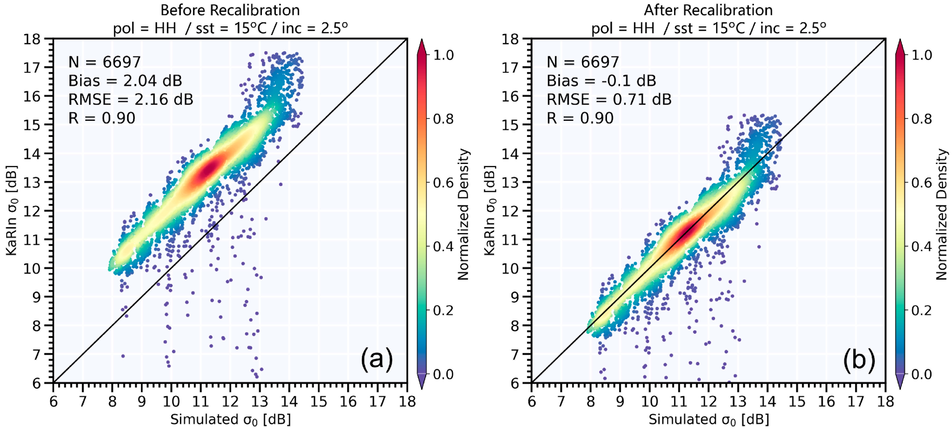
3. Analysis and Recalibration

Figure 3 plots two NRCS trends with collocated wind speeds from ECMWF at HH and VV polarizations. The yellow line is the fitting to KaRIn data, while the red line is the model from Global Precipitation Measurement (GPM) satellite Dual-frequency Precipitation Radar (DPR) data [25]. The corresponding incidence angle is 2.5°, while the SST is 15 °C. From the yellow fitting line in Figure 3a, we can observe that the KaRIn NRCS at VV polarization is sensitive to wind speed with a monotonically decreasing trend. This trend is consistent with the red model line. It reveals that the KaRIn data contain wind speed information like other radar data at low incidence angles. However, we can also see that there is a clear deviation between the two trends. We think this is due to calibration bias. Comparing these two types of radars (KaRIn and DPR), KaRIn has just been launched and the data are still being evaluated. The DPR radar data have been evaluated by many researchers since 2014. Therefore, we infer that the deviation is probably caused by the calibration error of KaRIn data.

Moreover, by comparing Figure 3a,b, the HH polarization data have similar characteristics to the VV polarization data in terms of wind speed sensitivity and NRCS deviation. This finding is consistent with previous findings [1,18]. This is because the scattering difference caused by the polarization factors is weak at low incidence angles.

Similar to Figure 3, Figure 4 plots the cases for other SST environments (8 °C, 23 °C and 30 °C) besides 15 °C. Figure 4a,c,d show that the KaRIn NRCS trends with wind speed are not exactly the same as those from the model. The trends of KaRIn and the model are consistent when wind speed and SST parameters are moderate. However, when the parameter values are relatively small or large, the differences between them are significant. For example, when the SST is 30 °C and the wind speed is 2 m/s, there is a deviation of approximately 1.5 dB from Figure 4d.

The calibration coefficient is independent of sea surface environmental parameters. It should remain constant for a fixed incidence angle and polarization. For the data characteristics presented in Figure 3 (the trends for the data and model are essentially the same), the deviation can be corrected easily using a recalibration coefficient. The recalibration coefficient C can be estimated as:

$${C=\sigma }_0^{\mathrm{o}\mathrm{r}\mathrm{i}}-{\sigma }_0^{\mathrm{m}}$$

(1)

where ${\sigma }_0^{\mathrm{o}\mathrm{r}\mathrm{i}}$ is the original KaRIn NRCS from download product, and the ${\sigma }_0^{\mathrm{m}}$ is the collocated model NRCS from DPR data.

However, as shown in Figure 4a,c,d, the deviations between the two trends for different SSTs are different. These differences are likely due to the electrical characteristics of the two radars. In this case, the direct use of Equation (1) may result in significant errors. Therefore, before using Equation (1), we selected the collocated KaRIn and model data with a high correlation to estimate the recalibration coefficient. The selection method consists of four steps. Three parameters (SST, incidence angle, and wind speed) were identified to construct multiple data bins. Next, the correlation coefficients between the two data bins (data and simulation) for different parameters were calculated. Third, the 10% of the data with the highest correlation coefficients were extracted separately and then intersected for different parameters. Finally, based on the selected data, the recalibration coefficients were estimated at different incidence angles using Equation (1).

Figure 5 presents the correlation coefficient trends with the SST, incidence angle, and wind speed for the HH and VV polarizations. Overall, the correlation coefficient fluctuates significantly with SST and wind speed, whereas it remains unchanged with the incidence angle.

From Figure 5a, the peak positions are mainly located at 8 °C, 15 °C and 23 °C, where it has a value of about 0.9. As shown in Figure 5b, the correlation coefficients are stable at approximately 0.85 at different incidence angles. As shown in Figure 5c, the correlation coefficient exhibits a downward parabolic characteristic with the wind speed. The value at the vertex can reach 0.73. Moreover, the HH and VV data have similar correlation coefficient characteristics, although that of the former is slightly higher than that of the latter. Based on the results in Figure 5, the data are extracted and intersected with the top 10% correlation coefficients.

Based on the selected data, the recalibration coefficients were estimated for each incidence angle, as shown in Figure 6. From the figure, both HH and VV recalibration coefficients are generally stable with the incidence angle, and the coefficient for VV polarization is approximately 0.3 dB higher than that for HH polarization.

Using the estimated recalibration coefficient, the KaRIn NRCS data for HH and VV polarizations were recalibrated according to the incidence angle. To evaluate the recalibration accuracy, the NRCS was compared between the KaRIn data and model simulations, as shown in Figure 7, in terms of bias, Root Mean Square Error (RMSE) and correlation coefficient (R). The used data are HH polarization, SST of 15 °C and incidence angle of 2.5°. The figure shows that the bias significantly improves from 2.04 dB to −0.1 dB.

Figure 4 is replotted in Figure 8 by replacing the results with recalibrated data. From the figure, we can observe that the trends between KaRIn and the model become more consistent than those before recalibration. Notably, consistency is mainly exhibited in the moderate wind speed range (4–16 m/s). There are still certain differences at both ends of the wind speed range. This is because the recalibration coefficients were estimated only using datasets with high correlation coefficients. This difference also indicates that with the DPR model it is difficult to fully describe KaRIn data characteristics, and a new model directly from KaRIn data should be developed. The next section introduces the development of the KaRIn GMF.

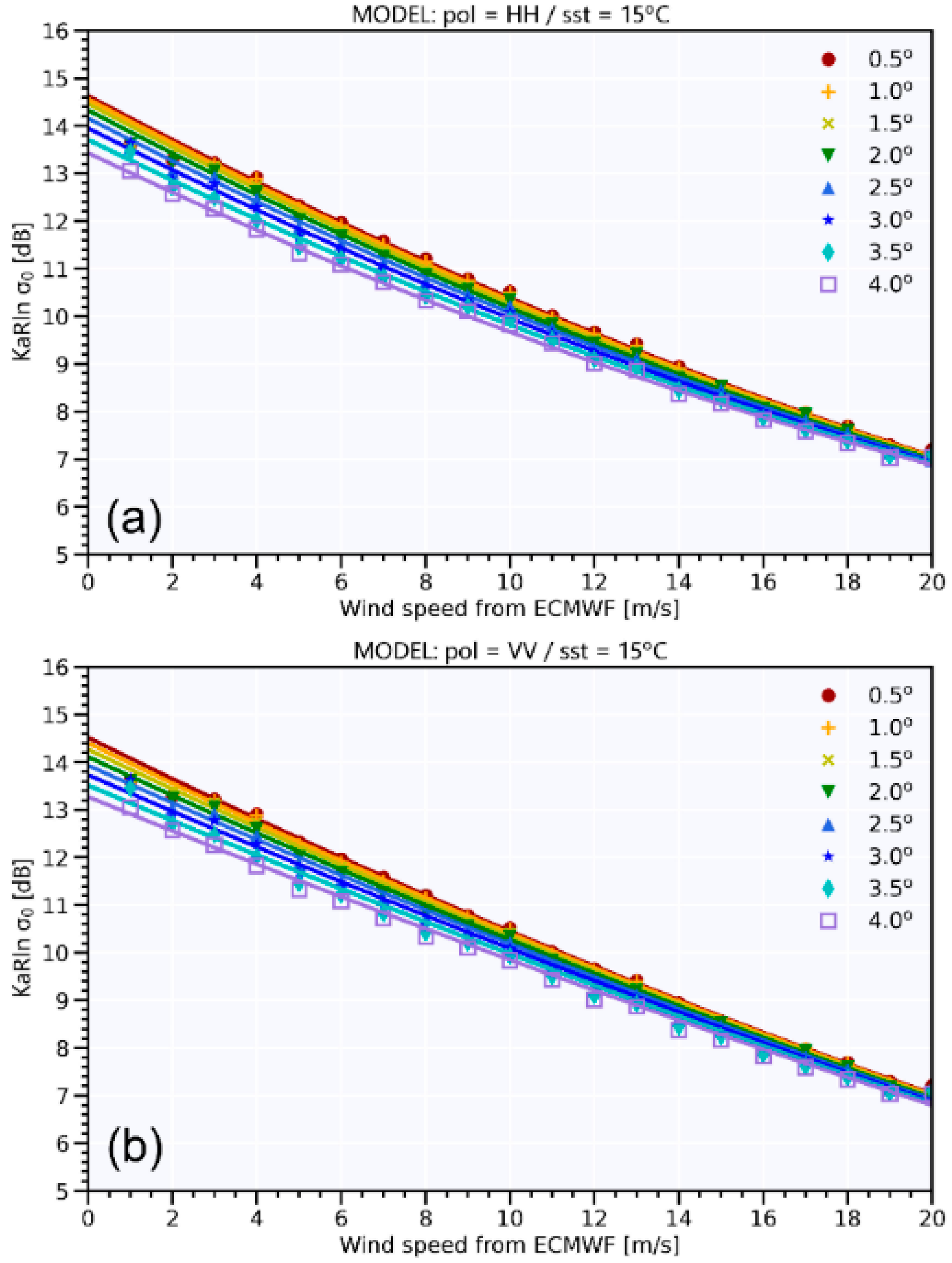
4. Model and Retrieval

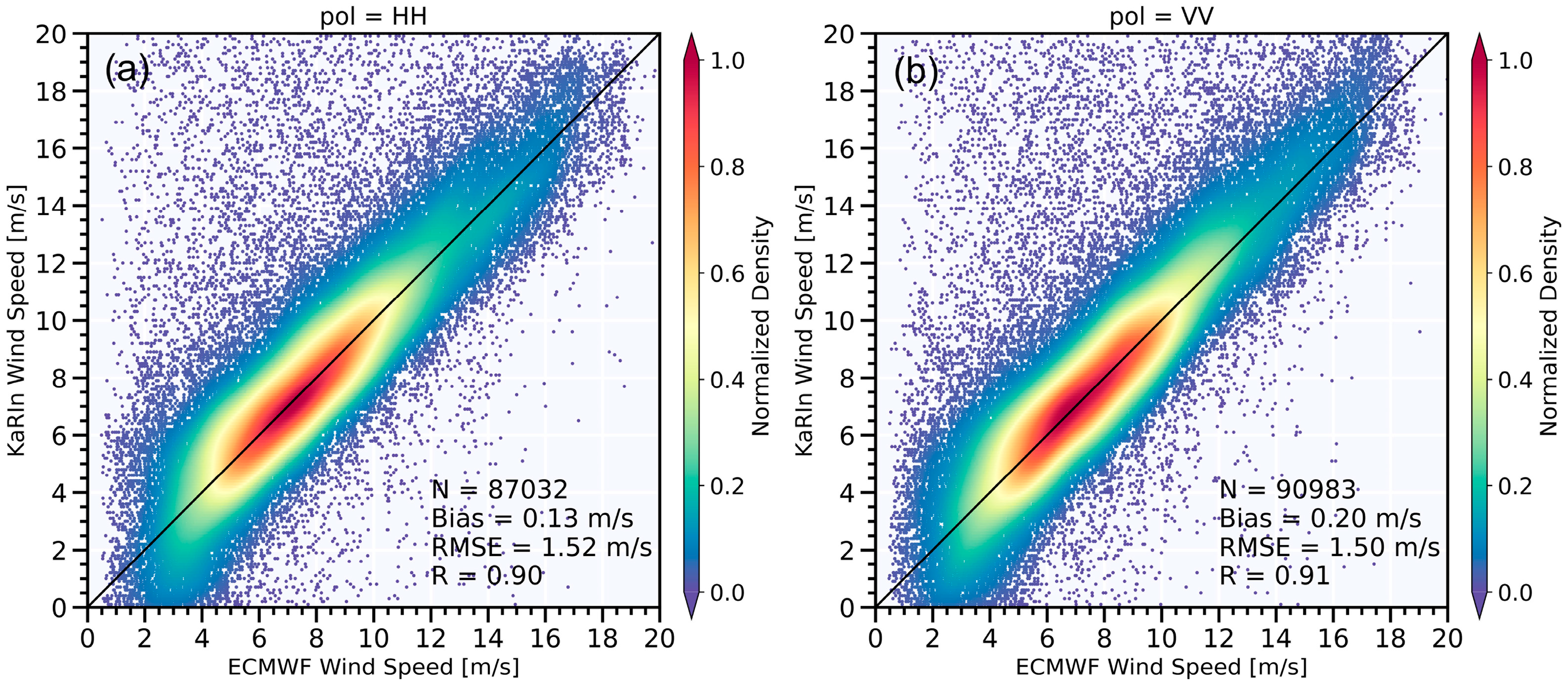
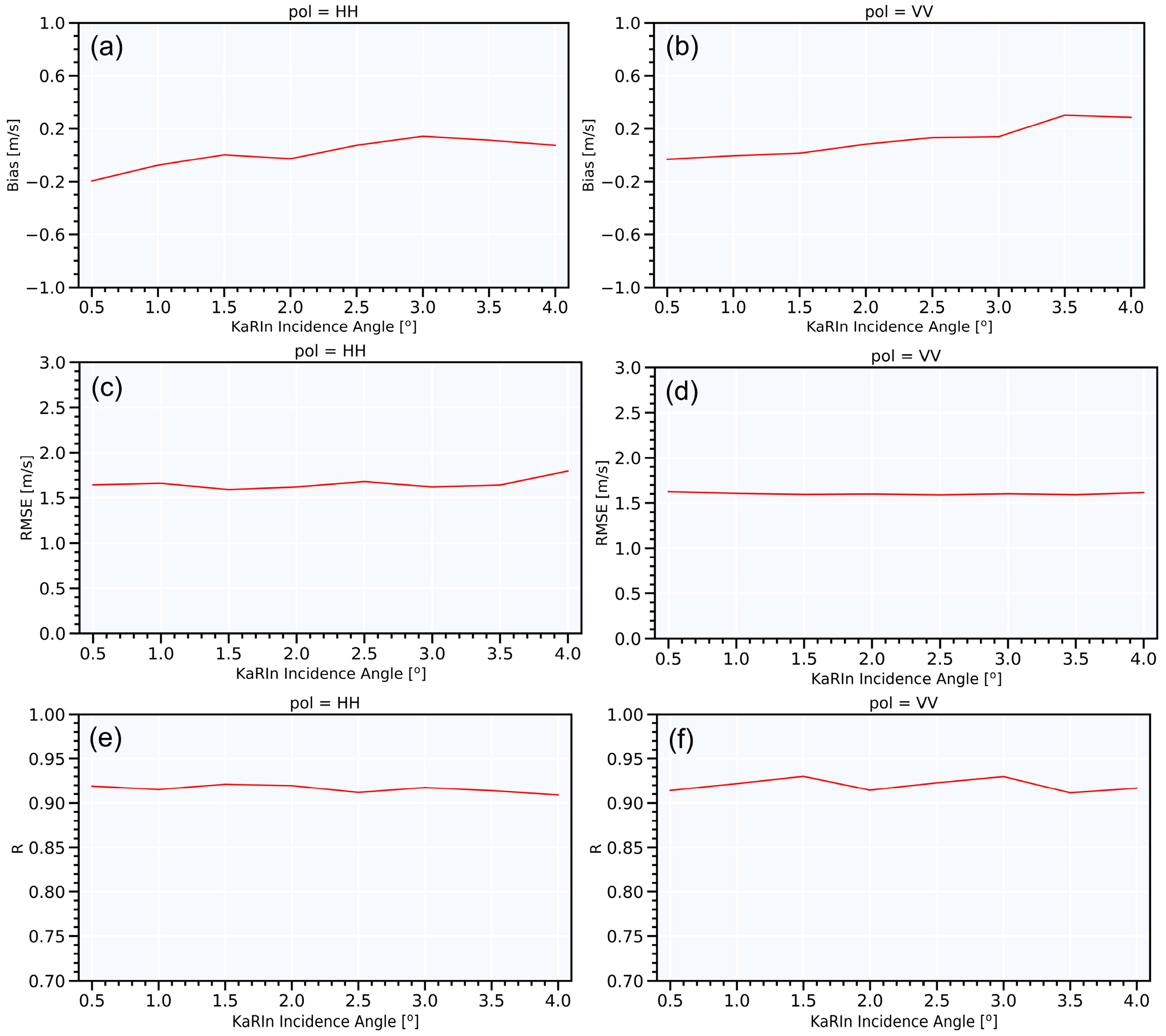
To describe the data characteristics better, we empirically developed a GMF using KaRIn data. According to previous studies [25,36,37], the Ka-band NRCS at low incidence angles is mainly related to SST, incidence angle and wind speed. Thus, the wind speed, SST and incidence angle were used as input parameters in the GMF. We utilized the same model structure as that of the DPR data [25] for the HH and VV. The model structure is as follows:

$${\sigma }_0\left(\theta ,u_{10},t,p\right)=a\left(\theta ,t,p\right)+b\left(\theta ,t,p\right)u_{10}+c\left(\theta ,t,p\right)u_{10}^2$$

(2)

Here,

$$a\left(\theta ,t,p\right)=a_0\left(t,p\right)+a_1\left(t,p\right)\theta +a_2\left(t,p\right){\theta }^2$$

(3)

$$b\left(\theta ,t,p\right)=b_0\left(t,p\right)+b_1\left(t,p\right)\theta +b_2\left(t,p\right){\theta }^2$$

(4)

$$c\left(\theta ,t,p\right)=c_0\left(t,p\right)+c_1\left(t,p\right)\theta +c_2{\left(t,p\right)\theta }^2$$

(5)

Here, ${\sigma }_0$ is KaRIn NRCS, $\theta$ is incidence angle, $u_{10}$ is the wind speed at 10 m sea surface height, t is SST at the center of the sea surface temperature segmentation, p is the polarizaiton and these parameters (a, b, c, a₀, a₁, a₂, b₀, b₁, b₂, c₀, c₁ and c₂) are model coefficients. The model coefficients were estimated by fitting the KaRIn data to the collocated data for the VV and HH polarizations. First, all the data were segmented using five SST values. Although SST can change the NRCS, the correlation is relatively weak compared with wind speed. Therefore, for convenience, a segmented model was adopted. Subsequently, a, b and c were estimated by fitting the NRCS to the wind speed in different segmented SST bins. Finally, a₀, a₁ and a₂ were estimated by fitting a to the incidence angle. b₀, b₁, b₂, c₀, c₁ and c₂ were estimated using a similar method. All estimated model coefficients for the HH and VV polarizations are listed in

Table 1. Model coefficients.

p	sst	a0	a1	a2	b0	b1	b2	c0	c1	c2
VV	1 °C	14.6133	−0.1665	−0.0420	−0.4482	0.0161	0.0014	0.0035	−0.0005	0.0000
	8 °C	14.7167	−0.0301	−0.0809	−0.4512	−0.0112	0.0082	0.0036	0.0007	−0.0000
	15 °C	15.7090	−0.1543	−0.0607	−0.6252	0.0111	0.0057	0.01156	−0.0003	−0.0001
	23 °C	15.8524	−0.0282	−0.1016	−0.6302	−0.0058	0.0132	0.0116	0.0002	−0.0005
	30 °C	15.4656	−0.2534	−0.0354	−0.5198	0.0709	−0.0078	0.0067	−0.0056	0.0010
HH	1 °C	14.6611	−0.0226	−0.0712	−0.4690	−0.0068	0.0045	0.0045	0.0003	−0.0001
	8 °C	14.7372	−0.07.91	−0.0784	−0.4569	0.0073	0.0051	0.0037	−0.0004	−0.0001
	15 °C	15.6130	−0.0270	−0.0973	−0.6084	−0.0057	0.0103	0.0106	0.0004	−0.0004
	23 °C	15.8815	0.0653	−0.1086	−0.6435	−0.0248	0.0125	0.0123	0.0013	−0.0004
	30 °C	14.6472	0.1518	−0.0989	−0.2719	−0.0709	0.0147	−0.0092	0.0054	−0.0008

.

Figure 9 presents models at HH and VV polarizations, which are plotted at an SST of 15 °C. From the figure, the KaRIn NRCS decreases with wind speed and incidence angle. As the wind speed increased, the NRCS modulation from the incidence angle weakened. Moreover, by comparing Figure 9a,b, although the two trends are generally consistent, there are still a few small differences. In the next retrieval step, wind speeds were retrieved from the KaRIn data using the developed GMF with VV and HH polarizations.

Using the developed GMF from the KaRIn data, wind speed $u_{10}$ can be retrieved by solving the minimum value of the cost function $\mathrm{J}$,

$$\mathrm{J}=\mathrm{a}\mathrm{b}\mathrm{s}\left[{\sigma }_0^{\mathrm{K}\mathrm{a}\mathrm{R}\mathrm{I}\mathrm{n}}-{\sigma }_0^{\mathrm{m}}\left(\theta ,u_{10},t,p\right)\right]$$

(6)

where ${\sigma }_0^{\mathrm{K}\mathrm{a}\mathrm{R}\mathrm{I}\mathrm{n}}$ is measured KaRIn NRCS. ${\sigma }_0^{\mathrm{m}}$ is simulated NRCS from the developed model. The incidence angle $\theta$, sea surface temperature t and polarization p are known.

In this study, the look-up table (LUT) method was used to estimate the wind speed solution in Equation (6). One-dimensional grids for wind speed, SST and incidence angle were first determined. The wind speed grids ranged from 0 m/s to 20 m/s at interval of 0.1. The SST grids ranged from 0 °C to 30 °C with an interval of 0.1. The incidence angle grids ranged from 0° to 4° with an interval of 0.1°. A combination of three types of grid points was introduced into the GMF to simulate the three-dimensional NRCS data.

The relationship between the input parameters and simulated NRCS constituted the LUT. When a set of wind speed, SST and incidence angle values is provided, the corresponding NRCS can be determined using the LUT. During wind speed retrieval, the NRCS and incidence angle were extracted from the KaRIn data, whereas the SST was extracted from the ECMWF data. In the process of retrieval, the $\theta$, t and p were first given. In this case, the wind speed grids and simulated NRCS grids were paired individually based on the LUT. The wind speed with the smallest difference between the KaRIn NRCS and the simulated NRCS was the final solution.

5. Evaluation

Three types of collocated data were used to evaluate the retrieved wind speeds: ECMWF, HY2C-SCAT and buoy data (NDBC and TAO). Figure 10 presents the wind speed comparisons between KaRIn retrievals and ECMWF collocations. From the figure, both the HH and VV retrievals are in good agreement with the collocated ECMWF wind speed data. Their biases are all close to zero, the RMSE for HH and VV data are 1.52 m/s and 1.50 m/s, respectively. Moreover, minor abnormal data deviates from the reference line. This is probably due to the data quality and rainfall.

Based on similar statistics, we analyzed the retrieval accuracy for each incidence angle bin from 0.5° to 4.0°, as shown in Figure 11. From the figure, the bias, RMSE and R are stable for the HH and VV data. The biases are smaller than 0.3 m/s, the RMSE are about 1.6 m/s, and the R are about 0.92.

Using similar evaluation methods on the ECMWF, the retrievals were also compared with the collocated HY2C-SCAT wind speed data, as shown in Figure 12 and Figure 13. From the comparisons, KaRIn retrievals at HH and VV polarizations and collocated HY2C-SCAT wind speed data are also consistent. As shown in Figure 12, the biases are smaller than 0.2 m/s for the HH and VV data, RMSEs are smaller than 1.34 m/s and both R values are 0.94. As shown in Figure 13, the bias, RMSE and R trends for the HH and VV data are also stable. The accuracy of the VV data is slightly higher than that of the HH data.

KaRIn retrievals were also compared with the collocated NDBC and TAO buoy wind speed data, as shown in Figure 14. The bias, RMSE and R at HH data are 0.23 m/s, 1.57 m/s and 0.88, respectively, while they are 0.18 m/s, 1.44 m/s and 0.88 for VV data. From the above statistics, the accuracies are basically consistent when KaRIn wind speed retrievals are compared to ECMWF, HY2C-SCAT and buoy winds.

6. Discussion

The main task of the KaRIn is to measure wide-swath SSH. As we know, the KaRIn SSH should have a high precision of centimeter level. Therefore, error correction for SSH is an important task. There are various errors introduced from the satellite itself, atmosphere and ocean. Sea-state bias is a typical error from ocean [38,39]. This bias is due to the fact that wave troughs have a stronger backscattering ability than wave peaks. Therefore, the sea surface estimated from the average scattering leaned towards the troughs, resulting in the estimated sea surface height being biased towards the troughs. The correction method for bias is based on collocated winds and waves. In this study, the wind speed retrieved from KaRIn itself was fully collocated with the SSH data. Therefore, we believe that wind speed retrieval by itself will have a better correction effect than the external wind speed products.

From the data analysis, an NRCS calibration bias was found in the KaRIn data by comparison with model simulations from the DPR data. We also found that wind trends from the KaRIn data and model simulations under different environments are not always consistent. Therefore, in the process of estimating recalibration coefficients, we did not use the entire dataset, but rather the highly correlated portion of the data between the KaRIn and the model to obtain a better calibration accuracy. This recalibration method using correlation analysis has rarely been reported in the literature, and it is recommended for wide application in the recalibration process of other radar data.

Many radar satellites, such as scatterometers, SAR and radiometers, have the ability to extract wind speed information. However, it is still very difficult to obtain global wind products with high temporal resolution based solely on a single satellite product. Therefore, multiple satellite products must be combined to obtain high-resolution data. In this study, KaRIn can also retrieve wind speeds similar to those of other wind sensors. Thus, KaRIn wind retrievals can be combined with other products to provide higher-temporal-resolution wind products.

According to previous studies, the NRCS at low incidence angles has very weak sensitivity at high wind speeds [40]. When the wind speed exceeded 20 m/s, the NRCS is basically constant with the wind speed. Owing to the non-sensitivity, high wind speeds have not been retrieved using NRCS data at a low incidence angle [20,23]. KaRIn operates at a low incidence angle and lacks the ability to retrieve high wind speeds. Joint applications with other wind sensors must be considered to achieve comprehensive wind speeds from low to high. In fact, all moderate incidence angle radars at copolarization always have the problem of high wind speed saturation (although the saturation effect is weaker than that of low incidence angle radars) [41,42]. To solve this problem, they utilized the unsaturated characteristics of the cross-polarization of wind speed to supplement the retrieval of high wind speeds [42,43,44]. This idea may also be applicable to low incidence angle radars, which use co-polarized data to measure low-to-moderate wind speeds and cross-polarization data to measure high wind speeds. At present, there are no low incidence angle radar test data for cross-polarization. We look forward to an opportunity to analyze the sensitivity of these data to high wind speeds in future work.

For the model developed in this study, in addition to the commonly used incidence angle and NRCS, SST was used as the input parameter. This is because Ka-band data are sensitive to SST [25,36,37]. Generally, changes induced by SST are not too drastic, and it is possible to use reanalysis data to provide SST. However, when encountering drastic changes from SST, higher time-resolution SST data are required to ensure the accuracy of wind speed retrievals. Currently, the SWOT satellite platform does not have the ability to observe SST in real time; therefore, there are still challenges in the accuracy of sea surface wind speed retrieval for rapidly changing sea surfaces. Possible solutions include carrying microwave radiometers or other optical temperature sensors on SWOT. These sensors, which can directly observe SST, can help the KaRIn radar further improve wind speed retrieval accuracy.

Traditional polynomial modeling methods were utilized in this study. With the rapid development of artificial intelligence technology, many studies in the field of ocean remote sensing retrieval have utilized artificial intelligence deep learning technology to develop retrieval models and algorithms [45,46]. Through deep learning of the sample library data, it is possible to discover new model input parameters and additional interactions between the observations and wind speed. Therefore, the use of emerging deep learning techniques can further improve the accuracy of wind speed retrieval. This is a step we plan to take in the future.

7. Conclusions

This study determined the wind speed sensitivity of SWOT KaRIn radar data and the calibration bias between KaRIn and the DPR model. Here, the DPR model was used as a reference to recalibrate the KaRIn NRCS. For recalibration, the KaRIn and simulated NRCS data with high correlation coefficients (maximum 10%) were used to estimate the recalibration coefficients, and a new model for VV and HH polarization was established using the recalibrated KaRIn data, which should describe the KaRIn data characteristics better than the DPR model. Using the new model, wind speed was retrieved from the recalibrated KaRIn data. These wind retrievals were evaluated using collocated ECMWF reanalysis winds, HY2C-SCAT winds and buoy (NDBC and TAO) winds. The results show that the wind retrievals are in good agreement with the collocated winds. All the RMSE are less than 1.57 m/s. Moreover, the bias, RMSE and R are constant with the incidence angles and polarizations.

References

1. Freilich, M.H.; Vanhoff, B.A. The relationship between winds, surface roughness, and radar backscatter at low incidence angles from TRMM precipitation radar measurements. J. Atmos. Ocean. Technol. 2003, 20, 549–562. [Google Scholar] [CrossRef]
2. Hersbach, H. Comparison of C-band scatterometer CMOD5.N equivalent neutral winds with ECMWF. J. Atmos. Ocean. Technol. 2010, 27, 721–736. [Google Scholar] [CrossRef]
3. Monaldo, F.; Jackson, C.; Li, X.; Pichel, W.G. Preliminary evaluation of sentinel-1a wind speed retrievals. IEEE J. Sel. Top. Appl. Earth Obs. Remote Sens. 2016, 9, 2638–2642. [Google Scholar] [CrossRef]
4. Brown, O.B.; Stanley, H.R.; Roy, N.A. The wind speed measurement capability of spaceborne radar altimetry. IEEE J. Ocean. Eng. 1981, 6, 59–63. [Google Scholar] [CrossRef]
5. Meissner, T.; Wentz, F.J. The emissivity of the ocean surface between 6 and 90 Ghz over a large range of wind speeds and earth incidence angles. IEEE Trans. Geosci. Remote Sens. 2012, 50, 3004–3026. [Google Scholar] [CrossRef]
6. Xu, H.; Han, C.; Wu, Y.; Sun, D.; Wang, X.; Li, J. A probability-constraint-based method for robust wind velocity estimation in lidar doppler spectrograms with low signal-to-noise ratio. IEEE Trans. Geosci. Remote Sens. 2023, 61, 5703310. [Google Scholar] [CrossRef]
7. Cox, C.; Munk, W. Measurement of roughness of the sea from photographs of the sun’s glitter. J. Opt. Soc. Am. 1954, 44, 838–850. [Google Scholar] [CrossRef]
8. Hwang, P.A.; Stoffelen, A.; Van Zadelhoff, G.J.; Perrie, W.; Zhang, B.; Li, H. Cross-polarization geophysical model function for c-band radar backscattering from the ocean surface and wind speed retrieval. J. Geophys. Res. Ocean. 2015, 120, 893–909. [Google Scholar] [CrossRef]
9. Mouche, A.; Chapron, B. Global C-band Envisat, RADARSAT-2 and Sentinel-1 SAR measurements in co-polarization and cross-polarization. J. Geophys. Res. Ocean. 2015, 120, 7195–7207. [Google Scholar] [CrossRef]
10. Portabella, M.; Stoffelen, A.; Johannessen, J.A. Toward an optimal inversion method for synthetic aperture radar wind retrieval. J. Geophys. Res. Ocean. 2001, 107, 3086. [Google Scholar] [CrossRef]
11. Ren, L.; Yang, J.; Mouche, A. Assessments of ocean wind retrieval schemes used for Chinese Gaofen-3 synthetic aperture radar co-polarized data. IEEE Trans. Geosci. Remote Sens. 2019, 57, 7075–7085. [Google Scholar] [CrossRef]
12. Stoffelen, A.; Verspeek, J.A.; Vogelzang, J. The CMOD7 geophysical model function for ASCAT and ERS wind retrievals. IEEE J. Sel. Top. Appl. Earth Obs. Remote Sens. 2017, 10, 2013–2124. [Google Scholar] [CrossRef]
13. Zhang, B.; Perrie, W.; Vachon, P.W.; Li, X.; Pichel, W.G.; Guo, J.; He, Y. Ocean vector winds retrieval from c-band fully polarimetric SAR measurements. IEEE Trans. Geosci. Remote Sens. 2012, 50, 4252–4261. [Google Scholar] [CrossRef]
14. Valenzuela, G.R. Theories for the interaction of electromagnetic and oceanic waves—A review. Bound.-Layer Meteorol. 1978, 13, 61–85. [Google Scholar] [CrossRef]
15. Gourrion, J.; Vandemark, D.; Bailey, S.; Chapron, B.; Gommenginger, G. A two-parameter wind speed algorithm for ku-band altimeters. J. Atmos. Ocean. Technol. 2002, 19, 2030–2048. [Google Scholar] [CrossRef]
16. Lillibridge, J.; Scharroo, R.; Abdalla, S. One- and two-dimensional wind speed models for ka-band altimetry. J. Atmos. Ocean. Technol. 2014, 31, 630–638. [Google Scholar] [CrossRef]
17. Yang, J.; Zhang, J.; Jia, Y.; Fan, C.; Cui, W. Validation of Sentinel-3A/3B and Jason-3 altimeter wind speeds and significant wave heights using buoy and ASCAT data. Remote Sens. 2020, 12, 2079. [Google Scholar] [CrossRef]
18. Tran, N.; Chapron, B.; Vandemark, D. Effect of long waves on Ku-band ocean radar backscatter at low incidence angles using TRMM and altimeter data. IEEE Geosci. Remote Sens. Lett. 2007, 4, 542–546. [Google Scholar] [CrossRef]
19. Chu, X.; He, Y.; Chen, G. Asymmetry and anisotropy of microwave backscatter at low incidence angles. IEEE Trans. Geosci. Remote Sens. 2012, 50, 4014–4024. [Google Scholar] [CrossRef]
20. Li, L.; Im, E.; Connor, L.N.; Chang, P.S. Retrieving ocean surface wind speed from the TRMM precipitation radar measurements. IEEE Trans. Geosci. Remote Sens. 2004, 42, 1271–1282. [Google Scholar] [CrossRef]
21. Ren, L.; Yang, J.; Zheng, G.; Wang, J. Wind speed retrieval from Ku-band tropical rainfall mapping mission precipitation radar data at low incidence angles. J. Appl. Remote Sens. 2016, 10, 016012. [Google Scholar] [CrossRef]
22. Ren, L.; Yang, J.; Jia, Y.; Dong, X.; Zheng, G. Sea surface wind speed retrieval and validation of the interferometric imaging radar altimeter aboard the Chinese tiangong-2 space laboratory. IEEE J. Sel. Top. Appl. Earth Obs. Remote Sens. 2018, 11, 4718–4724. [Google Scholar] [CrossRef]
23. Ren, L.; Yang, J.; Xu, Y.; Zhang, Y.; Zheng, G.; Wang, J.; Dai, J.; Jiang, C. Ocean surface wind speed dependence and retrieval from off-Nadir CFOSAT SWIM data. Earth Space Sci. 2021, 8, e2020EA001505. [Google Scholar] [CrossRef]
24. Panfilova, M.; Karaev, V. Wind speed retrieval algorithm using ku-band radar onboard GPM satellite. Remote Sens. 2021, 13, 4565. [Google Scholar] [CrossRef]
25. Jiang, C.; Ren, L.; Yang, J.; Xu, Q.; Dai, J. Wind speed retrieval using global precipitation measurement dual-frequency precipitation radar ka-band data at low incidence angles. Remote Sens. 2022, 14, 1454. [Google Scholar] [CrossRef]
26. Yang, J.; Ren, L.; Zheng, G. The first quantitative ocean remote sensing by using Chinese interferometric imaging radar altimeter onboard TG-2. Acta Oceanol. Sin. 2017, 36, 122–123. [Google Scholar] [CrossRef]
27. Zhang, Y.; Shi, X.; Wang, H.; Tan, Y.; Jiang, J. Interferometric Imaging Radar Altimeter on Board Chinese Tiangong-2 Space Laboratory. In Proceedings of the 2018 Asia-Pacific Microwave Conference (APMC), Kyoto, Japan, 6–9 November 2018; pp. 851–853. [Google Scholar]
28. Li, H.; Mouche, A.; Stopa, J.E.; Chapron, B. Calibration of the normalized radar cross section for sentinel-1 wave mode. IEEE Trans. Geosci. Remote Sens. 2019, 57, 1514–1522. [Google Scholar] [CrossRef]
29. Wang, H.; Li, H.; Lin, M.; Zhu, J.; Wang, J.; Li, D.; Cui, L. Calibration of the copolarized backscattering measurements from Gaofen-3 synthetic aperture radar wave mode imagery. IEEE J. Sel. Top. Appl. Earth Obs. Remote Sens. 2019, 12, 911–922. [Google Scholar] [CrossRef]
30. Fjørtoft, R.; Gaudin, J.M.; Pourthié, N.; Lalaurie, J.C.; Mallet, A.; Nouvel, J.F.; Martinot-Lagarde, J.; Oriot, H.; Borderies, P.; Ruiz, C.; et al. KaRIn on SWOT: Characteristics of near-nadir ka-band interferometric SAR imagery. IEEE Trans. Geosci. Remote Sens. 2014, 52, 2172–2185. [Google Scholar] [CrossRef]
31. Guo, H.; Wan, X.; Wang, H. Validation of just-released SWOT L2 Karin beta prevalidated data based on restore the marine gravity field and its application. IEEE J. Sel. Top. Appl. Earth Obs. Remote Sens. 2024, 17, 7878–7887. [Google Scholar] [CrossRef]
32. NASA JPL California Institute of Technolog and CNES. SWOT Product Description Level 2 KaRIn Low Rate Sea Surface Height Product (Revision A); NASA JPL California Institute of Technology and CNES: La Cañada Flintridge, CA, USA, 2022.
33. Sheng, Y.; Zhang, L.; Lin, M.; Zou, J.; Mu, B.; Peng, H. Evaluation of sea surface wind products from scatterometer onboard the Chinese HY-2D satellite. Remote Sens. 2023, 15, 852. [Google Scholar] [CrossRef]
34. Charnock, H. Wind stress on a water surface. Q. J. R. Meteorol. Soc. 1955, 81, 639–640. [Google Scholar] [CrossRef]
35. Smith, S.D. Coefficients for sea surface wind stress, heat flux, and wind profiles as a function of wind speed and temperature. J. Geophys. Res. 1988, 93, 15467–15472. [Google Scholar] [CrossRef]
36. Wang, Z.; Stoffelen, A.; Fois, F.; Verhoef, A.; Zhao, C.; Lin, M.; Chen, G. SST dependence of Ku- and C-band backscatter measurements. IEEE J. Sel. Top. Appl. Earth Obs. Remote Sens. 2017, 10, 2135–2146. [Google Scholar] [CrossRef]
37. Yan, Q.; Zhang, J.; Fan, C.; Meng, J. Analysis of Ku- and Ka-Band sea surface backscattering characteristics at low-incidence angles based on the GPM dual-frequency precipitation radar measurements. Remote Sens. 2019, 11, 754. [Google Scholar] [CrossRef]
38. Chelton, D.B. The sea state bias in altimeter estimates of sea level from collinear analysis of Topex data. J. Geophys. Res. Ocean. 1994, 99, 24995–25008. [Google Scholar] [CrossRef]
39. Miao, H.; Jing, Y.; Jia, Y.; Lin, M.; Zhang, G.; Wang, G. Nonparametric estimations of the sea state bias for a radar altimeter. Acta Oceanol. Sin. 2017, 36, 108–113. [Google Scholar] [CrossRef]
40. Li, X.; Zhang, B.; Mouche, A.; He, Y.; Perrie, W. Ku-band sea surface radar backscatter at low incidence angles under extreme wind conditions. Remote Sens. 2017, 9, 474. [Google Scholar] [CrossRef]
41. Zhang, B.; Zhu, Z.; Perrie, W.; Tang, J.; Zhang, J.A. Estimating tropical cyclone wind structure and intensity from spaceborne radiometer and synthetic aperture radar. IEEE J. Sel. Top. Appl. Earth Obs. Remote Sens. 2021, 14, 4043–4050. [Google Scholar] [CrossRef]
42. Mouche, A.A.; Chapron, B.; Zhang, B.; Husson, R. Combined co- and cross-polarized SAR measurements under extreme wind conditions. IEEE Trans. Geosci. Remote Sens. 2017, 55, 6746–6755. [Google Scholar] [CrossRef]
43. Vachon, P.W.; Wolfe, J. C-Band cross-polarization wind speed retrieval. IEEE Geosci. Remote Sens. Lett. 2011, 8, 456–459. [Google Scholar] [CrossRef]
44. Zhang, G.; Li, X.; Perrie, W.; Hwang, P.A.; Zhang, B.; Yang, X. A hurricane wind speed retrieval model for C-Band RADARSAT-2 cross-polarization ScanSAR images. IEEE Trans. Geosci. Remote Sens. 2017, 55, 4766–4774. [Google Scholar] [CrossRef]
45. Liu, S.; Li, Y.; Zhou, W.; Jin, X.; Yang, X.; Dou, H.; Li, H. Ocean surface parameters estimation from microwave radiometer voltages using deep learning. IEEE Trans. Geosci. Remote Sens. 2024, 62, 5300813. [Google Scholar] [CrossRef]
46. Cao, C.; Bao, L.; Gao, G.; Liu, G.; Zhang, X. A novel method for ocean wave spectra retrieval using deep learning from Sentinel-1 wave mode data. IEEE Trans. Geosci. Remote Sens. 2024, 62, 4204016. [Google Scholar] [CrossRef]
Figure 1. Location map for SWOT KaRIn data and collocated HY2C-SCAT, NDBC buoy and TAO buoy wind data. Here, the red points indicate positions of collocations for KaRIn and HY2C-SCAT data. The green plus signs indicate the NDBC buoy positions. The blue multiple signs indicate the TAO buoy positions. The period for KaRIn data is from 6 September 2023 to 21 November 2023.
Remotesensing 16 03103 g001
Figure 2. Data distribution of ECMWF data for (a) wind speed and (b) sea surface temperature data.
Remotesensing 16 03103 g002
Figure 3. KaRIn NRCS trends with the wind speeds from ECMWF at (a) VV polarization and (b) HH polarization. Here, the gold line indicates the fitting line for KaRIn NRCS observations, while the red line indicates the model line. The incidence angle is 2.5° and the collocated sea surface temperature is 15 °C.
Remotesensing 16 03103 g003
Figure 4. KaRIn NRCS trends with the wind speeds from ECMWF at different sea surface temperatures of (a) 8 °C, (b) 15 °C, (c) 23 °C and (d) 30 °C. The incidence angle is 2.5°.
Remotesensing 16 03103 g004
Figure 5. Correlation coefficient trends with sea surface temperatures (a,b), incidence angles (c,d) and wind speeds (e,f). Here the left column is for HH polarization, while the right column is for VV polarization.
Remotesensing 16 03103 g005
Figure 6. The KaRIn recalibration coefficient trends with the incidence angles at HH and VV polarizations.
Remotesensing 16 03103 g006
Figure 7. NRCS comparisons between the KaRIn data and the model simulations. (a) Before recalibration and (b) after recalibration.
Remotesensing 16 03103 g007
Figure 8. Recalibrated KaRIn NRCS trends with the wind speeds from ECMWF at different incidence angles of (a) 0.5°, (b) 1.5°, (c) 2.5° and (d) 3.5°. The collocated sea surface temperature is 15 °C.
Remotesensing 16 03103 g008
Figure 9. GMF models developed by the recalibrated KaRIn NRCS data at (a) HH polarization and (b) VV polarization.
Remotesensing 16 03103 g009
Figure 10. Wind speed comparisons between KaRIn retrievals and collocations from ECMWF at (a) HH polarization and (b) VV polarization.
Remotesensing 16 03103 g010
Figure 11. Bias, RMSE and R trends with incidence angles by comparing KaRIn retrievals with ECMWF wind speeds. (a,c,e) HH polarization; (b,d,f) VV polarization.
Remotesensing 16 03103 g011
Figure 12. Wind speed comparisons between KaRIn retrievals and collocations from HY2C-SCAT at (a) HH polarization and (b) VV polarization.
Remotesensing 16 03103 g012
Figure 13. Bias, RMSE and R trends with incidence angles by comparing KaRIn retrievals with HY2C-SCAT wind speeds. (a,c,e) HH polarization; (b,d,f) VV polarization.
Remotesensing 16 03103 g013
Figure 14. Wind speed comparisons between KaRIn retrievals and collocations from NDBC buoy at (a) HH polarization and (b) VV polarization.
Remotesensing 16 03103 g014