Infrared Camera Array System and Self-Calibration Method for Enhanced Dim Target Perception

Abstract

Camera arrays can enhance the signal-to-noise ratio (SNR) between dim targets and backgrounds through multi-view synthesis. This is crucial for the detection of dim targets. To this end, we design and develop an infrared camera array system with a large baseline. The multi-view synthesis of camera arrays relies heavily on the calibration accuracy of relative poses in the sub-cameras. However, the sub-cameras within a camera array lack strict geometric constraints. Therefore, most current calibration methods still consider the camera array as multiple pinhole cameras for calibration. Moreover, when detecting distant targets, the camera array usually needs to adjust the focal length to maintain a larger depth of field (DoF), so that the distant targets are located on the camera’s focal plane. This means that the calibration scene should be selected within this DoF range to obtain clear images. Nevertheless, the small parallax between the distant sub-aperture views limits the calibration. To address these issues, we propose a calibration model for camera arrays in distant scenes. In this model, we first extend the parallax by employing dual-array frames (i.e., recording a scene at two spatial locations). Secondly, we investigate the linear constraints between the dual-array frames, to maintain the minimum degrees of freedom of the model. We develop a real-world light field dataset called NUDT-Dual-Array using an infrared camera array to evaluate our method. Experimental results on our self-developed datasets demonstrate the effectiveness of our method. Using the calibrated model, we improve the SNR of distant dim targets, which ultimately enhances the detection and perception of dim targets.

1. Introduction

Camera arrays capture both the intensity and direction of light rays [1] and enable the synthesis of multiple perspectives to enhance the signal-to-noise ratio (SNR) between spatial dim targets and backgrounds [2], thereby enhancing the detection capability for dim targets [3]. This method addresses the limitations of traditional techniques in adapting to changes in illumination and complex backgrounds [4], while also circumventing the data requirements and computational resource dependencies associated with deep-learning-based approaches [5,6].

The commercialization of light field (LF) imaging devices has accelerated the development of LF technology. Common LF imaging devices can be categorized into three distinct types based on their structural design: scanning LF cameras [7,8,9], microlens-array-based LF cameras (also known as plenoptic cameras) [10,11,12], and camera arrays [13,14,15]. Scanning LF cameras require stability of the LF throughout the capture process, which limits their applicability to dynamic scenes [8]. Plenoptic cameras have a limited overall resolution, and therefore must trade-off between spatial and angular resolution of captured LF images [16]. Existing camera arrays are typically bulky and expensive [17], and most still operate in the visible spectral range.

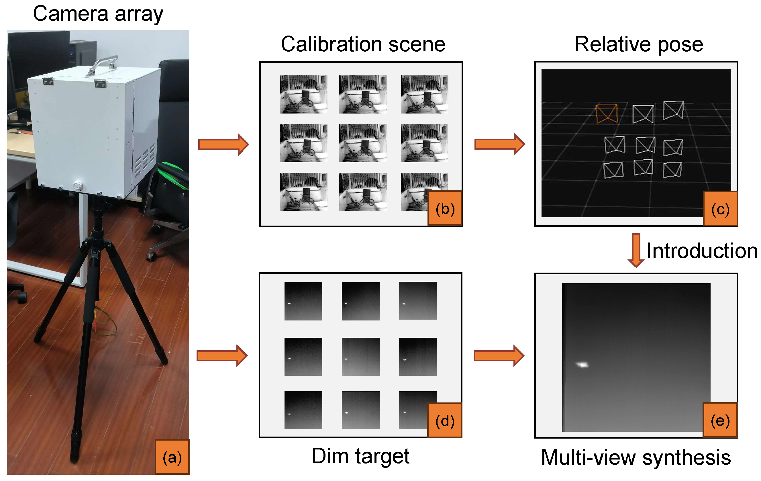
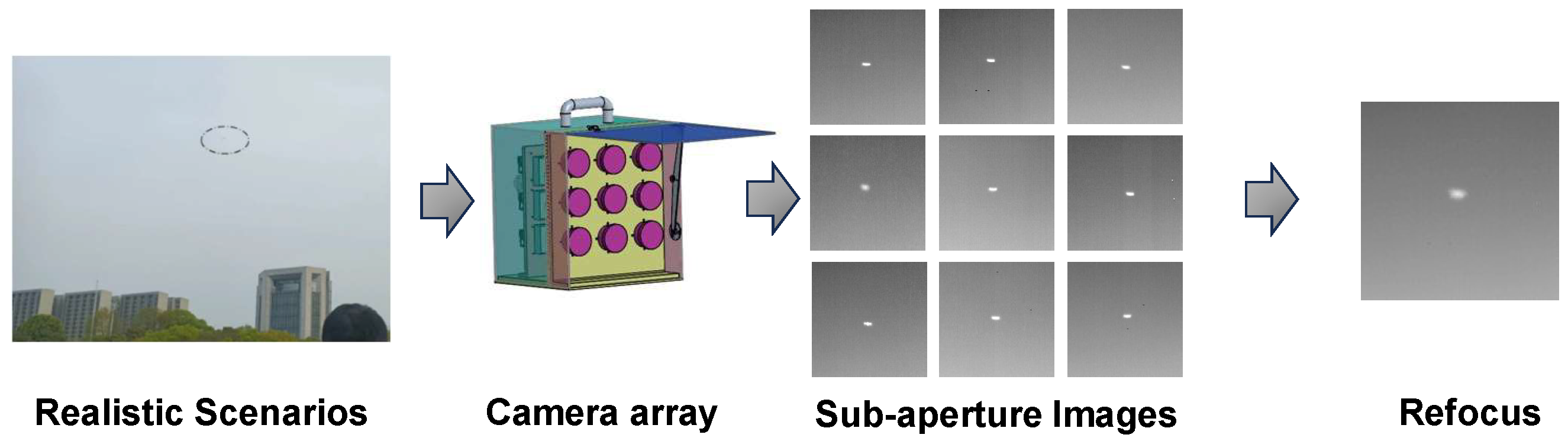
To address the structural limitations of conventional LF imaging devices for tasks such as dim target detection, this paper introduces a novel infrared camera array system (as shown in Figure 1). The infrared camera array we designed offers excellent mobility, highly synchronized image acquisition accuracy, impressive baseline depth resolution, and the ability to detect dim targets in the long-wave infrared spectrum (LWIR). The camera array fulfills the requirement to capture moving dim targets under a wide range of conditions, which eliminates the limitations of traditional LF imaging equipment.

The calibration of camera arrays is critical for LF imaging and spatial dim target perception. Extensive research has been conducted across various domains, including 3D target localization [18], full optical camera calibration [19], spatial position and pose measurement [20], target position measurement [21], and robot visual measurement [22]. 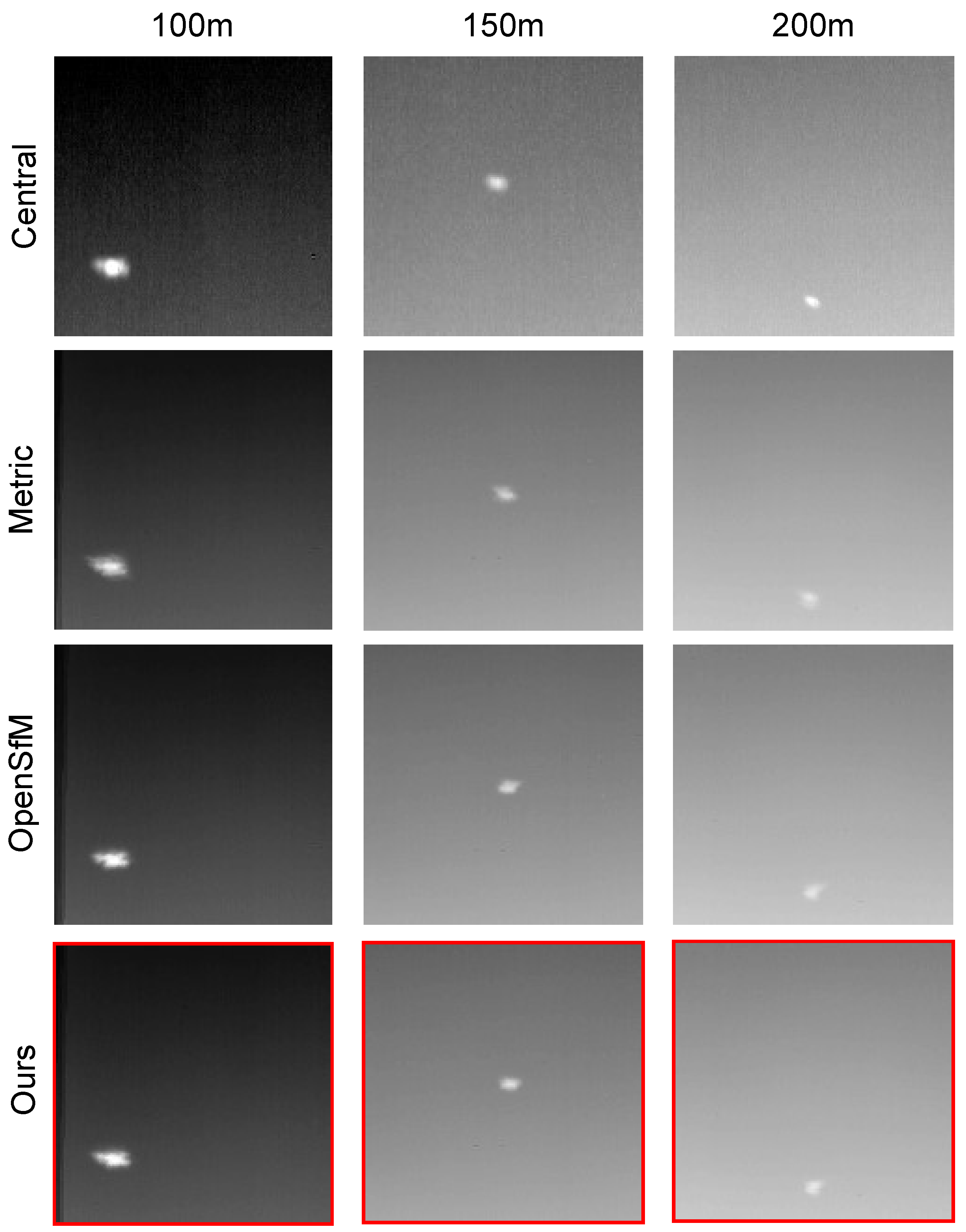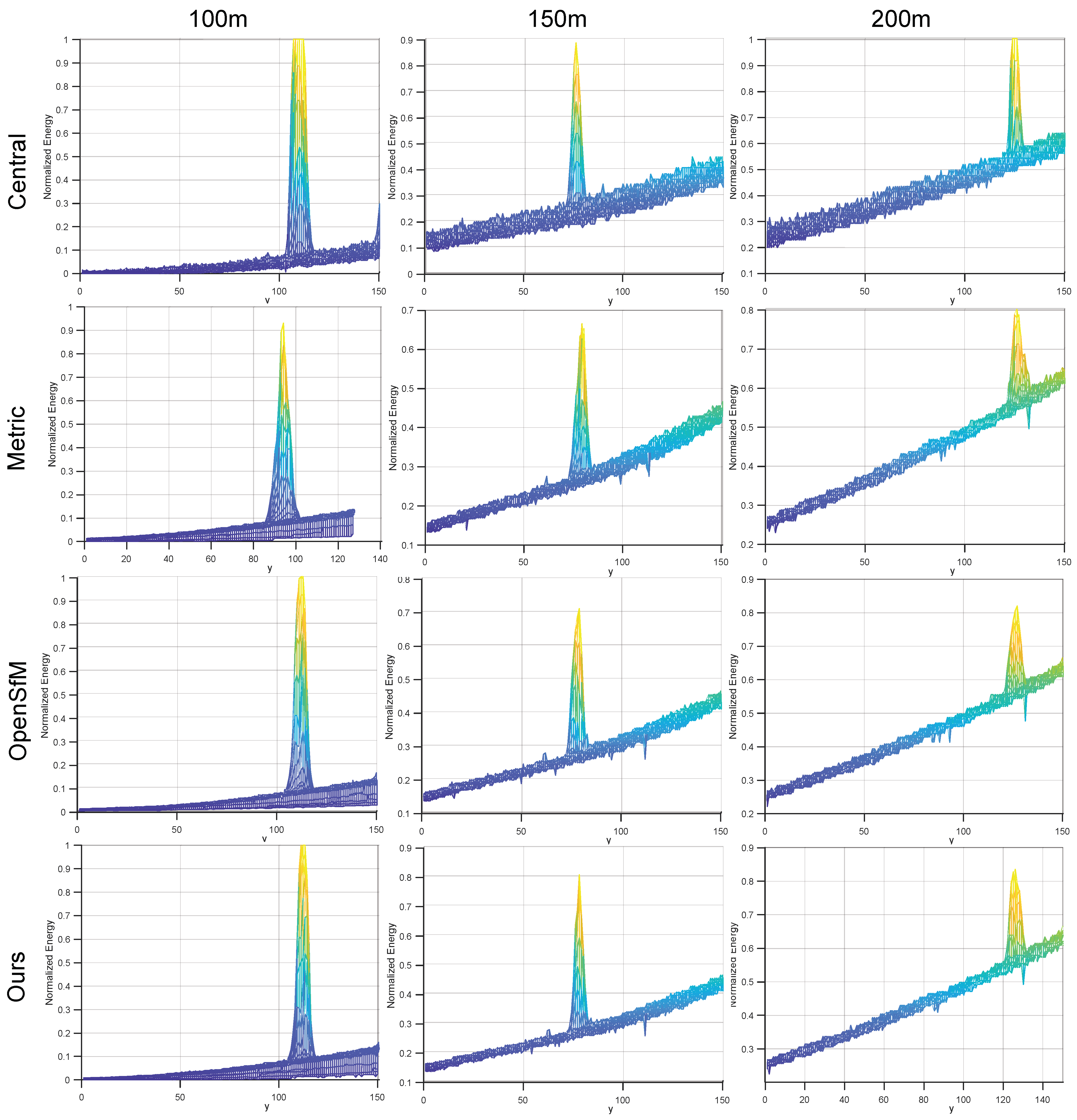The calibration of camera arrays involves considerations of pose [23,24] and disparity [25,26] for each camera viewpoint. Numerous calibration methods have been developed to meet the diverse requirements of different applications. 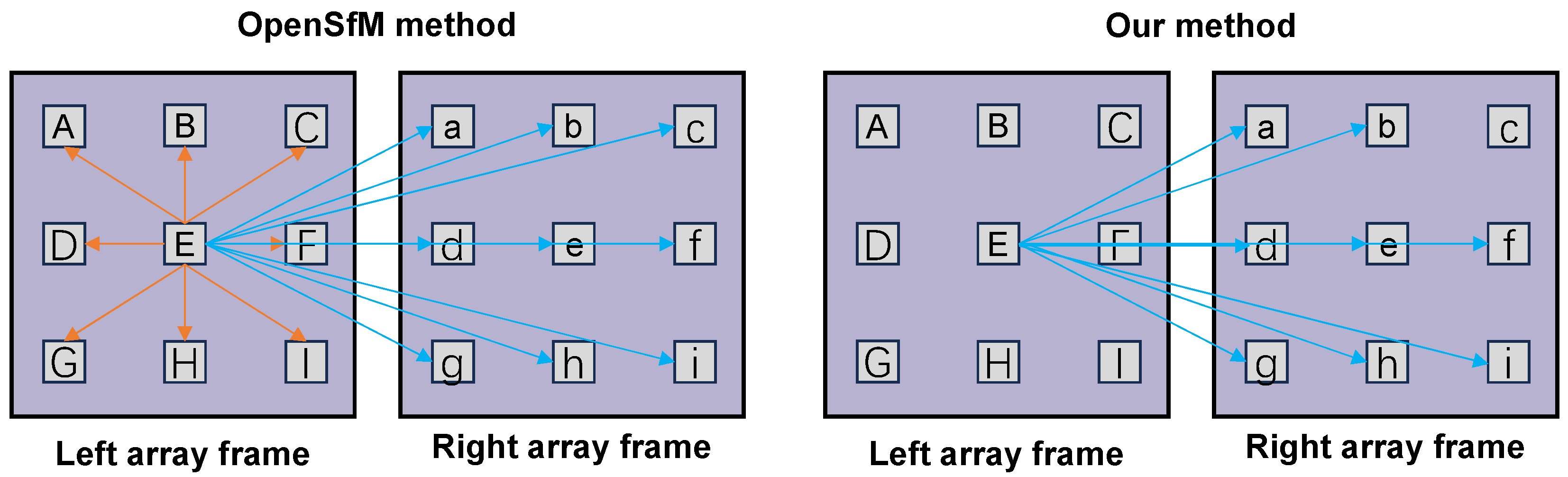While current methods, such as metric calibration [27] and structure-from-motion (SfM)-based method [28], have made considerable progress, they still treat the camera array as a combination of pinhole cameras, and the geometrical constraints that exist between sub-cameras have not been investigated, which leads to unsatisfactory calibration accuracy. In addition, the infrared camera arrays we designed faced unique challenges. Since the camera array is used to detect dim targets at long distances, its sub-cameras capture clear images at infinity by adjusting their focal lengths. Therefore, during the calibration process, the calibration scene should also be chosen far enough away so that the camera array can capture a calibrated scene with sharp texture details. However, choosing a calibration scene that is too far away can lead to parallax deficiency problems, so the rays reconstructed from a single array frame are very dense and easily corrupted by noise.

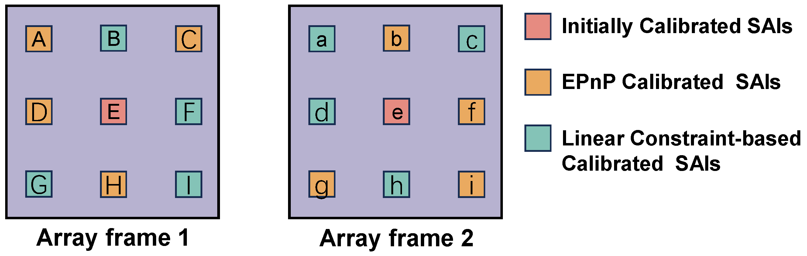
To address this problem, we propose a comprehensive calibration model. The model enhances the discrepancy by capturing the scene twice at different spatial locations, thus extending the spatial resolution of the LF. In addition, the model derives a set of linear constraints regarding the ray space correspondence between dual-array frames. This maintains the minimum degrees of freedom of the model by adding orderly sub-aperture images (SAIs) and effectively reduces the cumulative reprojection error due to the addition of LF images.

In this paper, our goal is to provide a high-precision self-calibration method for infrared camera arrays to achieve dim target perception, as shown in Figure 1. The main contributions of this paper can be briefly described as follows:

(1)

We design an innovative infrared camera array system to provide a novel solution for open world dim target detection.

(2)

We propose a comprehensive calibration model for the infrared camera array. This model establishes linear constraints on the ray space correspondence within the camera array at two different spatial positions.

(3)

We develop a real-world LF dataset for comprehensive performance evaluation. In addition, guided by the obtained camera poses, we achieve dim target SNR enhancement based on multi-view synthesis.

The remaining sections of the paper are structured as follows. Section 2 provides an overview of previous related work. In Section 3, we introduce our own designed and developed infrared camera array, which demonstrates its advantages in visual perception and target detection. Section 4 proposes a self-calibration method for the infrared camera array. Section 5 presents experimental results on real-world data, which demonstrate the accuracy and robustness of the proposed self-calibration method compared to state-of-the-art methods. Section 6 discusses the application prospects and existing problems of the designed infrared camera array and its self-calibration model in practical tasks, which provides direction for our next research efforts. Finally, Section 7 concludes the paper.

2. Related Works

Recently, advances in camera array technology have attracted great interest in various fields such as machine vision, robotics, and virtual reality. In the field of 3D reconstruction, camera arrays demonstrate the potential to capture depth information of the scene and provide powerful support for generating 3D models [29,30]. In addition, camera arrays have a variety of applications in target measurement [31], target tracking [32,33], light field refocusing [34], and super-resolution reconstruction [35].

2.1. Camera Arrays Development

Depending on the purpose and structure, camera arrays can be classified into different types, including stereoscopic, multi-view, or LF systems. These systems consist of multiple cameras arranged in specific configurations to capture multi-dimensional images or video of the same scene from various viewpoints. Regarding different shapes of camera arrays, researchers have proposed various types, such as planar camera arrays [14,36,37], circular camera arrays [38,39,40], and spherical camera arrays [41,42,43], to meet different application needs. Planar camera arrays were originally designed to capture LF information [44,45] and contributed to the development of LF cameras [46]. While LF cameras can capture the intensity and direction of light through microlenses to obtain angular information about the scene, they are limited by the resolution of the sensor, which requires the operator to choose between dense spatial sampling or angular sampling [12]. In contrast, planar camera arrays provide better image resolution by mounting multiple independent cameras on a regularly shaped structure. However, planar camera arrays currently lack the capability to detect, track, and identify distant, small, and dim targets effectively. Therefore, there is an urgent need for the development of equipment to promote the advancement of related technology.

2.2. LF Relative Pose Estimation

As a type of LF imaging device, camera arrays exhibit strong similarities in terms of imaging effects and calibration methods with LF cameras. Moreover, research on the calibration of LF cameras is extensive and relatively mature. Therefore, studying the current state of LF camera calibration is very helpful for our research.

In recent years, many pose estimation algorithms for LF cameras have been developed to leverage their unique characteristics, resulting in improved performance. Pless [47] defined a generalized camera model as a set of rays and established correspondences between rays intersecting the same 3D point, known as the generalized epipolar constraint (GEC). Considering all degenerate camera configurations, Li et al. [48] employed a linear algorithm to solve the relative pose from the GEC efficiently without ambiguities, which is also applicable to LF cameras. Johannsen et al. [49] were the first to introduce the GEC into LF cameras and considered the geometric constraints between projections within a single LF, effectively utilizing the characteristics of LF cameras. Zhang et al. [50] investigated how the ray manifolds associated with geometric features, including points, lines, and planes, transform when the relative pose changes and exploited these transformations to recover the pose. Nousias et al. [51] proposed a complete pipeline of LF SfM where the approach to pose estimation is the same as [48]. Zhang et al. [52] established the homography in ray space between two LF cameras and used rays captured by the two LF cameras to solve the relative pose.

However, the rays extracted from LF images using a small baseline are highly dense and susceptible to noise corruption in the aforementioned methods. To mitigate the drawbacks associated with rays, Nousias et al. [53] introduced an LF projection matrix to encapsulate the correspondence between LF features and 3D points, employing direct linear transformation (DLT) to estimate the absolute pose of LF cameras. The LF features used are directly derived from LF images. Nevertheless, the precision of the recovered 3D points may still be compromised by the limited baseline. In the latest research [54], a model of LF-point-LF-point correspondence was established, detailing the relationship between LF features (LF-points) extracted from a pair of LF raw images. This model eliminates the need for 3D points. During the resolution of this model, the rotation and translation were separated and addressed individually. The relative pose is represented by the LF-point components and the intrinsic parameters of the LF camera. In this article, we propose a comprehensive calibration model for the infrared camera array. This model establishes linear constraints on the ray space correspondence within the camera array at two different spatial positions. By doing so, it maintains the minimum degrees of freedom for the model.

3. Design and Construction of Infrared Camera Array System

3.1. System Composition and Principle

As shown in Figure 2, the 3 × 3 infrared camera array system measures 270 × 251.3 × 50 mm externally. It is made up of nine non-cooled LWIR cameras, four five-port gigabit switches, three GPUs, and a power supply module.

Each LWIR camera consists of a lens with adjustable back focus and a detector. They are mounted as a unit on a bracket. A set of three cameras share a five-port gigabit switch and GPU, which are combined in one unit and powered by a power module.

The power supply module receives 12 V of external power and converts it to the voltage required by each component to ensure proper operation. Eight LWIR cameras operate simultaneously, triggered by the exposure signal from one camera. All nine LWIR cameras capture images of the external scene at a consistent exposure time and frame rate.

The image processing module processes three streams of image data, compresses and streams the data, and sends it to the host computer through the switch. When a store command is received, it transfers the raw camera data to the storage module. The storage module then writes these data to a storage card. The continuous image storage time is greater than 30 min at 50 Hz. The data can be exported and deleted through the PC management system.

The 3 × 3 infrared camera array system’s main specifications are listed in

Table 1. Proposed infrared camera array system.

Item	Infrared Camera Array System
Camera Array Scale	3 × 3
Response Waveband	8–14 $\mathsf{\mu }\mathrm{m}$
Optical Focal Length	35 mm (±5%)
Lens F Number	F/0.8
Single Camera Pixel Size	640 × 512
Pixel Pitch	12 $\mathsf{\mu }\mathrm{m}$
Frame Rate	50 Hz
Dynamic Range	0–200 °C
Quantization Bit Depth	14 bit
Frame Synchronization Precision	5 ms
Light Axis Consistency	2 pixels
Continuous Image Storage Duration	>30 min@50 Hz
Continuous Stable Working Time	>12 h
Operating Environment Temperature	−20–50 °C
Power Consumption	150 W
Volume	<350 mm × 300 mm × 300 mm
Weight	<10 kg
Power Supply Type	12 V

.

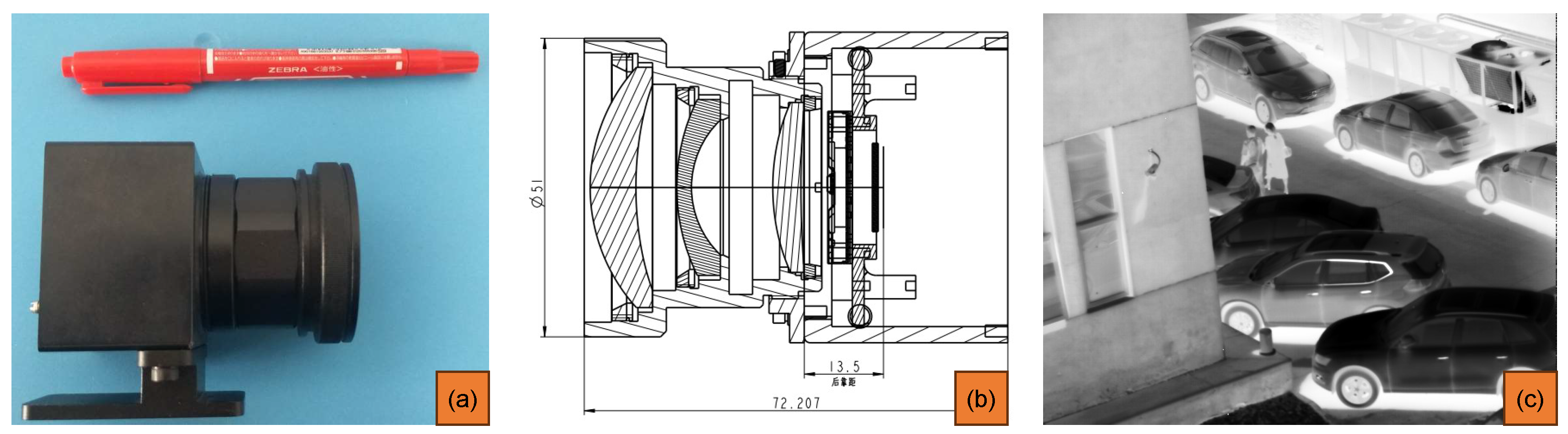
3.2. Non-Cooled LWIR Camera Design Proposal

The camera features a non-cooled LWIR sensor and a lens. Figure 3 shows the hardware design of this camera, and its main specifications are listed in

Table 2. Proposed non-cooled LWIR camera.

Item	Non-Cooled LWIR Camera
Detector Material	Alum Oxide
Response Waveband	8–14 $\mathsf{\mu }\mathrm{m}$
Detector Elements	640 × 512
Pixel Pitch	12 $\mathsf{\mu }\mathrm{m}$
Detector Origin	China
Optical Focal Length	35 mm (±5%), F/0.8
Frame Rate	50 Hz
Effective Field of View	Azimuth: 8.80°, Elevation: 7.04°
External Synchronization	TTL Signal

.

The optical system is a passive non-thermalized optical structure. It consists of three lenses made of sulfur glass and zinc selenide (ZnSe). The total length of the optical system is 50 mm, the total weight is about 63.2 g, and the back focal length is greater than 14 mm. The detector’s pixel size is 12 $\mathsf{\mu }\mathrm{m}$× 12 $\mathsf{\mu }\mathrm{m}$, with a Nyquist spatial frequency of about 1/(2 × 12 $\mathsf{\mu }\mathrm{m}$) ≈ 40 lp/mm. The modulation transfer function (MTF) value at 40 lp/mm is over 0.4, and the energy concentration exceeds 0.3.

Due to the fact that a temperature change will cause refractive index changes, optical materials and lens barrel materials undergo thermal expansion. This causes the optical system to defocus, which affects the image quality of the system. Therefore, the system uses aluminium alloy as the lens barrel material (the coefficient of thermal expansion is about 23.6 × ${10}^{-6}$/K). At the same time, we consider the mechanical structure and the effect of the optical components on the image quality when subjected to temperature changes. Through the reasonable combination of different materials, the system can meet the image quality requirements from low temperatures (−20 °C) to high temperatures (50 °C).

The optical system consists of five lenses. The surface of each lens is coated with a transmittance enhancement film. The transmittance of a single piece can reach 97%, and the total transmittance of the optical system is $\tau$ = 0.973. The rear flange is connected to the detector, and the flange is connected to the lens by threads so that the rear leaning distance can be fine-tuned and locked by three set screws around the circumference.

3.3. Function and Specification of the System

The infrared camera array and image acquisition system is primarily used for high-frame-rate imaging of specific application scenarios. The system can control camera imaging parameters, synchronize image data acquisition, provide real-time display previews, and store and retrieve data. Image acquisition between sub-cameras requires high time synchronization accuracy and a consistent output frame rate. The control and image data readout interfaces for the camera array are designed with versatility in mind and have the ability to store and replay raw data. Its main technical indicators are shown in Table 1.

4. Infrared Camera Array Self-Calibration Method

Our goal is to improve the detection capability of spatial dim targets by synthesizing multi-view array images. The infrared camera array’s calibration accuracy directly impacts the multi-view synthesis’s effectiveness. Therefore, we propose a comprehensive self-calibration model for the infrared camera array (as shown in Figure 4). First, this model extends the spatial resolution of the LF by capturing a scene at two spatial locations (i.e., dual-array frames). Then, we derive a set of linear constraints regarding the correspondence of ray space between the dual-array frames and maintain the minimum necessary degrees of freedom for the calibration model. Additionally, we also introduce an initial pair adaptive selection strategy to provide a set of precise initial 3D points for our self-calibration model.

4.1. Dual-Array Frames Acquisition

Our method utilizes dual-array frames to calibrate the infrared camera array. Specifically, the initial array frame is acquired by recording a scene from the first perspective. Then, the second array frame is acquired through the parallax–baseline relationship:

$$d={\displaystyle \frac{b·f}{Z}},$$

(1)

where f is the focal length, d represents the difference between images (parallax), and Z represents the depth of the object from the camera array. The baseline b required for the dual array frames can be calculated through these three easily obtainable parameters. Subsequently, the infrared camera array is moved to the second perspective for recording.

4.2. Correspondence Graph Build

The second stage of our pipeline focuses on constructing a correspondence graph, which involves four steps [55].

4.2.1. Feature Extraction and Intra-Frame Matching

For dual-array frames, sparse feature points are detected using the difference of Gaussian (DoG) [56] corner measurement method, and their RootSIFT descriptors [57] are computed. Standard distance ratio testing [56] is used to match the RootSIFT descriptors of the central SAI with those of other SAIs. Only matching feature sets that appear in at least four SAIs are retained.

4.2.2. Inter-Frame Matching

For efficiency, only the descriptors of the central SAI are used for matching. Combining ratio testing with left–right consistency checks, correspondences between frame pairs are determined. Since descriptors between different LF viewpoints are expected to have low similarity, a more lenient threshold is used for the ratio test. The five-point algorithm [58] is used within the RANSAC framework to fit an essential matrix, and outliers are discarded.

4.2.3. Establishing Multi-Frame Matches

Starting from the correspondences determined in the previous step, a directed graph is constructed, where each vertex represents a matching feature, and each pair of vertices represents a feature pair. This process ultimately identifies a list of feature matches for the same 3D points across multiple array frames.

4.3. Initial Two-View Reconstruction

To compute the initial reconstruction using two images, there needs to be enough parallax between them. Fachada et al. [59] propose to use the central image of a multi-array image to determine the initial image pair. However, since the shooting position of the multi-array image is human-controlled, the use of the central image as the initial image pair results in a non-optimal parallax between the two views, which leads to poor triangulation results. In OpenSfM [60], an adaptive initial image pairs selection method is proposed. It starts by trying to fit a rotation-only camera model to the two images. It only considers image pairs that have a significant portion of the correspondences that cannot be explained by the rotation model. It computes the number of outliers of the model and accepts it only if the portion of outliers is larger than 30%. However, this method does not consider the characteristics of multi-array images, so it is necessary to iterate through all the images to determine the rotation model. As shown on the left side of Figure 5, every image needs to fit the rotation-only camera model 17 times, so the computation time is long.

In our calibration model, a dual-array frame is used to expand the parallax. Therefore, the selection of the initial image pair only needs to be considered from the across array frames. As shown on the right side of Figure 5, every image needs to fit the rotation-only camera model eight times. Specifically, we select two images from different array frames, and their matched point pairs are ${\mathbf{p}}_{Array1}$$=\{{\mathbf{p}}_{Array1,1},\dots ,{\mathbf{p}}_{Array1,i},\dots ,{\mathbf{p}}_{Array1,N}\}$ and ${\mathbf{p}}_{Array2}=\{{\mathbf{p}}_{Array2,1},\dots ,{\mathbf{p}}_{Array2,i},\dots ,{\mathbf{p}}_{Array2,N}\}$. The disparity is calculated by fitting a rotation matrix to the two SAIs using the five-point algorithm [58]. Then, the feature points of the right SAI ${\mathbf{p}}_{Array2}$ are transformed to the coordinate system of the left SAI:

$${\mathbf{p}}_{rect,i}=\mathbf{R}·{{\mathbf{p}}_{Array2,i}}^T\forall i\in N,$$

(2)

where ${{\mathbf{p}}_{Array2,i}}^T$ represents the transpose matrix of ${\mathbf{p}}_{Array2,i}$, $\mathbf{R}$ denotes the rotation matrix, and ${\mathbf{p}}_{rect,i}$ denotes the rectified feature point. Then, the disparity between the two SAIs is calculated according to:

$$dis{p}_i=\sqrt{{\displaystyle \sum _{k=1}^d}{({\mathbf{p}}_{rect,i}\left(k\right)-{\mathbf{p}}_{Array1,i}\left(k\right))}^2}\forall i\in N,$$

(3)

where $dis{p}_i$ represents the disparity between ${\mathbf{p}}_{rect,i}$ and ${\mathbf{p}}_{Array1,i}$, and d is the dimension of the points. Subsequently, feature points with a disparity larger than the threshold value are labeled as outliers. Then, an index list of outliers is obtained. We compute the number of outliers of the model and accept it only if the portion of outliers is larger than 30% (the same as OpenSfM [60]). The accepted image pairs are sorted by the number of outliers of the rotation-only model. Finally, two-view pose calibration and bootstrap reconstruction are performed based on the optimal initial pair.

4.4. Incremental Reconstruction

After achieving good initial reconstruction and pose calibration, we integrate the remaining SAIs incrementally. The camera array consists of multiple pinhole lenses, and there are no specific geometric constraints between the projections within a single LF. However, since our calibration model adopts a dual-array frame, we studied the geometric constraints between the projections of the camera array within the LF composed of dual-array frames. Ultimately, a dual-array frame linear constraint estimator is proposed. This linear constraint estimator reduces reliance on the 2D–3D pose solution of the perspective-n-point (PnP) method [61], thereby enhancing the robustness of pose calibration.

Specifically, as shown in Figure 6, assume that images A and a comprise the initial image pair, and their absolute poses ${\mathbf{P}}_A=[{\mathbf{R}}_A|{\mathbf{t}}_A]$ and ${\mathbf{P}}_a=[{\mathbf{R}}_a|{\mathbf{t}}_a]$ have been calibrated in the previous section using the 2D-2D method. Next, assume that the absolute pose ${\mathbf{P}}_B=[{\mathbf{R}}_B|{\mathbf{t}}_B]$ of image B is calibrated based on the 2D–3D efficient perspective-n-point (EPnP) method [62]. Then, we can calculate the relative pose between image A and image B:

$$\left[{\mathbf{R}}_1|{\mathbf{t}}_1\right]={\mathbf{P}}_B^{-1}·{\mathbf{P}}_A=\left[{\mathbf{R}}_B^T{\mathbf{R}}_A|{\mathbf{R}}_B^T({\mathbf{t}}_B-{\mathbf{t}}_A)\right].$$

(4)

According to the principle that the relative pose of the camera array remains unchanged before and after two shots, we can know that the relative pose obtained from images a and b is also $\left[{\mathbf{R}}_1|{\mathbf{t}}_1\right]$. Ultimately, we can calculate the absolute pose of image b through the linear constraint between the dual-array frames as:

$${\mathbf{P}}_b=\left[{\mathbf{R}}_a|{\mathbf{t}}_a\right]·\left[{\mathbf{R}}_1|{\mathbf{t}}_1\right]=\left[{\mathbf{R}}_a{\mathbf{R}}_1|{\mathbf{R}}_a{\mathbf{t}}_1+{\mathbf{t}}_a\right]$$

(5)

The algorithm proposed by us is shown in Algorithm 1.

Algorithm 1 Dual-array frame linear constraint pose estimate method

Input: SAIs feature points $\mathbf{p}$; The initially reconstructed 3D points; Initial image pair absolute poses ${\mathbf{P}}_A$ and ${\mathbf{P}}_a$ Output: SAIs absolute poses   1:  for Uncalibrated images remain do   2:     EPnP [62] calibrate one SAI absolute pose ${\mathbf{P}}_i$   3:     Perform local Bundle Adjustment (BA) optimization and re-triangulation   4:     if The corresponding image of ${\mathbf{P}}_i$ in another array frame is uncalibrated then   5:       Compute the relative pose between ${\mathbf{P}}_i$ and ${\mathbf{P}}_A$ (or ${\mathbf{P}}_a$) by Equation (4)   6:       Calibrate the pose of the corresponding image in another array frame based on linear constraints by Equation (5)   7:       Perform local BA optimization and re-triangulation   8:     else   9:       Continue  10:    end if  11: end for  12: return SAIs absolute poses

A calibration result of our proposed method is shown in Figure 7. We analyzed the effectiveness of our method in addressing cumulative reprojection errors. While the EPnP algorithm [62] is a commonly used and efficient method for camera pose estimation, its limitations and sensitivity to various factors may lead to errors. However, by integrating our proposed method, we can obtain the pose of an unknown view from the known view’s pose through the matrix’s linear operation. Therefore, this approach reduces the model’s degrees of freedom and thus suppresses the cumulative reprojection errors.

5. Experiments

To comprehensively study the proposed method, we conducted extensive experiments for evaluation. In Section 5.1, we obtain the experimental parameters and construct a dual-array frame dataset using our infrared camera array. In Section 5.2, we comprehensively evaluate our calibration model compared to state-of-the-art approaches. In Section 5.3, we evaluate the execution time of our calibrated model. In Section 5.4, we conduct experiments on dim target SNR enhancement using the poses obtained from our calibration model. By comparing the SNR of refocused dim targets, we finally validate the effectiveness of our proposed infrared camera array system and self-calibration method.

5.1. Acquisition of Experimental Parameters and Construction of Dataset

To evaluate the performance of the proposed pose calibration method, it is first necessary to obtain the intrinsic parameters of each sub-camera of the infrared camera array. Secondly, it is also essential to construct a suitable dataset for its evaluation.

5.1.1. Acquisition of Intrinsic Parameters

Since the infrared camera array consists of nine long-wave LWIR sub-cameras, we designed a thermostatically controlled heating chessboard to obtain high-precision intrinsic parameters. As shown in Figure 8, the thermostatically controlled heating checkerboard measures 1.5 × 2 m and features a 14 × 10 grid pattern and a heating module to maintain a constant temperature. It can present high-quality patterns in the view of the infrared camera array.

Specifically, through rotation and translation, we obtain 15 images of the checkerboard grid with different poses. These images were then fed into the Camera Calibrator toolbox in matlab, and the intrinsic parameters (as shown in

Table 3. The intrinsic parameters of the infrared camera array (pixel).

Num	${\mathit{f}}_{\mathit{x}}$	${\mathit{f}}_{\mathit{y}}$	${\mathit{c}}_{\mathit{x}}$	${\mathit{c}}_{\mathit{x}}$	${\mathit{K}}_1$	${\mathit{K}}_2$
1	2765.33	2765.21	264.67	132.64	−0.15	7.18
2	2736.96	2736.24	234.54	110.62	0.19	0.38
3	2696.24	2696.41	306.88	166.90	−0.31	24.91
4	2716.73	2717.15	256.03	94.12	−0.01	−5.87
5	2703.07	2704.70	238.08	104.41	−0.10	−16.03
6	2725.08	2724.96	293.52	120.73	−0.03	−7.36
7	2736.01	2736.14	278.08	93.17	−0.04	−5.98
8	2705.35	2706.76	284.03	91.35	−0.17	10.22
9	2684.96	2688.74	301.01	88.30	−0.10	−6.36

) of the infrared camera array were derived according to Zhang’s method [27]. Figure 9 shows the accuracy of the calibrated intrinsic parameters, with the mean reprojection error (MRE) for all nine lenses being less than 0.12 pixels.

5.1.2. Construction of Self-Developed Dataset

We constructed an infrared dual-array frame dataset to evaluate the proposed method. Specifically, we first selected four scenes with abundant details, where the distance between the objects and the camera array is 15–30 m. Calibrating at this distance ensures that the sub-cameras are clear at infinity. Then, we captured four scenes at two different spatial locations according to Section 4.1. Finally, we constructed a dual-array frame dataset, as shown in the first row of Figure 10.

5.2. Calibration Model Evaluation

In this section, we comprehensively evaluate our calibration model in comparison with state-of-the-art approaches. Firstly, in the initial two-view reconstruction stage, we evaluate the effect of the adaptive initial image pair selection strategy proposed. Then, in the incremental reconstruction stage, we compare the final calibration results of the proposed self-calibration model with COLMAP [28] and OpenSfM [60] and thereby validate the gain brought by introducing linear constraints between the dual-array frames. Finally, we perform a scene reconstruction comparison with COLMAP and OpenSfM on real images.

5.2.1. Initial Two-View Pose Calibration and Reconstruction Comparison

In this stage, we demonstrate the results of two-view reconstruction using three initial image pair selection methods (i.e., Fachada et al.’s [59] method, the OpenSfM [60] method, and our method) in four scenes. In

Table 4. Initial two-view pose calibration and reconstruction comparison.

Scenes	Initial Image Pair			Two-View Inliers			Triangulated			Time
	[59]	[60]	Ours	[59]	[60]	Ours	[59]	[60]	Ours	[59]	[60]	Ours
Bike	$\mathit{E}$–$\mathit{e}$	$\mathit{a}$–$\mathit{i}$	$\mathit{F}$–$\mathit{e}$	254/317	446/479	200/271	210	57	215	-	0.094 $\mathrm{s}$	0.056$\mathrm{s}$
Robot	$\mathit{E}$–$\mathit{e}$	$\mathit{F}$–$\mathit{H}$	$\mathit{C}$–$\mathit{h}$	78/107	208/239	205/232	68	219	228	-	0.269 $\mathrm{s}$	0.185$\mathrm{s}$
Mind	$\mathit{E}$–$\mathit{e}$	$\mathit{C}$–$\mathit{I}$	$\mathit{D}$–$\mathit{g}$	71/131	722/752	588/607	0	335	533	-	0.261 $\mathrm{s}$	0.175$\mathrm{s}$
Sculpture	$\mathit{E}$–$\mathit{e}$	$\mathit{F}$–$\mathit{g}$	$\mathit{C}$–$\mathit{c}$	201/318	765/797	141/264	46	31	122	-	0.115 $\mathrm{s}$	0.086 $\mathrm{s}$

, we first present the selection of the initial image pair under different methods (refer to the numbers in Figure 8). Then, we evaluate the methods based on the number of inliers of the two views, the number of triangulated points, and the algorithm runtime. The boldfaced entries indicate the best results, while the underlined entries represent the second-best results. Specifically, Fachada et al.’s [59] method triangulates near the maximum number of points in the Bike scene, but fails to triangulate in the Mind scene. This is because the Fachada et al. [59] method fixes the use of the central SAI of the dual-array frame as the initial image pair ($\mathit{E}$–$\mathit{e}$). This method is limited by the quality of the acquired dual-array frames. In addition, this method determines the initial image pair by specifying the image, so its running time is 0. The OpenSfM [60] method determines the initial image pair for a rotation-only camera model. Therefore, it performs best in terms of inliers. However, its selection of initial image pairs are all concentrated in the same array frame, which still suffers from insufficient parallax. It leads to a smaller number of final triangulated points than our method. This method also has the longest running time compared to our method. When acquiring dual-array frame images, we artificially control the images to have good parallax between the dual-array frames. Therefore, our method is set to determine the initial image pairs across array frames. The initial image pair selected by our method from the across array frames matches a small number of inliers, but its final triangulation has the largest number of points. This is because our method balances between inliers and parallax. Moreover, our method has the shortest running time.

5.2.2. Incremental Pose Calibration and Reconstruction Comparison

In this stage, we compare the performance of the proposed method with COLMAP [28] and OpenSfM [60]. Specifically, during the experimental process, we first ensure that we use the same feature extraction and matching methods. Then, we conduct high-quality auto-reconstruction experiments in four scenes using COLMAP [28]. Next, since the OpenSfM [60] parameters are adjustable, we conduct three sets of experiments under different min-track lengths (MTL), where MTL is an important parameter in SfM, affecting the reconstruction quality and processing speed. Finally, experiments with our method are conducted based on linear constraints in dual-array frames.

In terms of performance evaluation, due to the absence of ground truth for the relative poses of the camera array, we reproject the reconstructed 3D points onto all SAIs to calculate the mean reprojection error (MRE) according to:

$$MRE={\displaystyle \frac{1}{N}}{\displaystyle \sum _{i=1}^N}\sqrt{{(x_{proj,i}-x_{GT,i})}^2+{(y_{proj,i}-y_{GT,i})}^2},$$

(6)

where $(x_{GT,i},y_{GT,i})$ represents a real image point, $(x_{proj,i},y_{proj,i})$ represents a reprojected point, and N represents the number of reconstructed 3D points.

Our experimental results are presented in

Table 5. Comparison of MRE ↓ (pixel).

Methods	Bike	Robot	Mind	Sculpture
COLMAP [28]	0.66	0.68	0.52	0.71
OpenSfM-MTL(2) [60]	0.79	0.62	0.53	0.66
OpenSfM-MTL(4) [60]	0.88	0.71	0.57	0.69
OpenSfM-MTL(6) [60]	0.86	0.74	0.69	0.72
Ours	0.57	0.65	0.46	0.62

. Experimental results show that our proposed method consistently maintains the minimum MRE in all four scenes. Compared to the previous improvements, it has been increased by up to 35.2%. This demonstrates the effectiveness of introducing linear constraints in the dual-array frame.

5.2.3. Structure Estimation Quality Comparison

In addition, we conducted quality comparison experiments for structure estimation. We visually evaluate the quality of pose calibration by displaying the structures recovered in four scenes using three methods. Specifically, as shown in Figure 10, the overall structure estimated by COLMAP [28] in the four scenes is not good. OpenSfM [60] estimates structure details less effectively than our method. These visual results are consistent with the conclusions in Table 5.

5.3. Execution Time Comparison

The introduction of linear constraints on the dual-array frames allows the calibration model to maintain a minimum number of degrees of freedom and improves computational efficiency. Therefore, in this stage, we perform a comparison of execution times. Specifically, we perform pose calibration in each of the four scenes.

Table 6. Execution time comparison.

Scenes	COLMAP [28]	OpenSfM [60]	Ours
Bike	37.86 $\mathrm{s}$	25.52 $\mathrm{s}$	21.56 $\mathrm{s}$
Robot	35.93 $\mathrm{s}$	28.70 $\mathrm{s}$	21.58 $\mathrm{s}$
Mind	23.41 $\mathrm{s}$	23.91 $\mathrm{s}$	19.86 $\mathrm{s}$
Sculpture	29.31 $\mathrm{s}$	27.58 $\mathrm{s}$	21.25 $\mathrm{s}$

demonstrates the comparison of the three methods in execution time. Our method achieves the shortest running time since the introduction of linear constraints, with an average improvement of 31.8%. This validates the industrial practicality of our proposed calibration model.

5.4. Enhanced Dim Target SNR Experiment

To validate the effectiveness of the infrared camera array system and its self-calibration methods for dim target perception, the experiment of enhancing the SNR of dim targets is conducted in this stage using the poses provided by the three calibration methods. The metric calibration method [27] is the most commonly used checkerboard-grid-based calibration method. The OpenSfM [60] method and our method are the self-calibration methods that were verified well in the previous section.

5.4.1. Evaluation Metrics

Wu et al. [2] introduced an infrared image noise theory and analyzed the advantages of multi-view synthetic aperture imaging in improving the SNR of dim targets. Specifically, the SNR after multi-view synthesis is calculated according to:

$$SNR=E_t/E_n,$$

(7)

$$E_t={\displaystyle \sum _{i\in I}}|I_{res}\left(i\right)|/|T|,$$

(8)

$$E_n={\displaystyle \sum _{i\in U\setminus T}}|I_{res}\left(i\right)|/(|U|-|T|),$$

(9)

$E_t$ is the energy of the target, $E_n$ is the noise energy, $I_{res}$ is the residual image after background suppression, T is the set of image elements occupied by the target, and U is the set of full image elements. U and T denote the number of image elements in the set, respectively. Wu et al. [2] stated that the noise in the synthetic aperture image obeys the distribution $\overline{n}\sim N\left(0,{\displaystyle \frac{{\sigma }^2}{K}}\right)$, so calculating the spatial average of the noise energy can be equated to calculating the expectation of the noise energy, i.e.,

$$\begin{array}{ll}{E}_n& ={\displaystyle \sum _{i\in U\setminus T}}|I_{res}\left(i\right)|/(|U|-|T|)=E(|n|)\\ & =\underset{-\infty }{\overset{+\infty }{\int }}\left|x\right|{\displaystyle \frac{\sqrt{K}}{\sqrt{2\pi }\sigma }}{e}^{-{\displaystyle \frac{K{x}^2}{2{\sigma }^2}}}dx={\displaystyle \frac{\sqrt{2K}}{\sqrt{\pi }\sigma }}\underset{0}{\overset{+\infty }{\int }}x{e}^{-{\displaystyle \frac{K{x}^2}{2{\sigma }^2}}}dx\\ & =\sqrt{{\displaystyle \frac{2}{K\pi }}}\sigma ={\displaystyle \frac{C_1}{\sqrt{K}}},\end{array}$$

(10)

where $C_1$ is a constant. It is known from the above equation that the noise energy is inversely proportional to the 0.5 power of the number of cameras. The target energy remains constant in the synthetic imaging process, so

$$SNR={\displaystyle \frac{E_t}{E_n}}={\displaystyle \frac{E_t}{\sqrt{C_1}}}\sqrt{K}.$$

(11)

By theoretical derivation, the SNR of the image obtained by synthetic aperture imaging is proportional to the 0.5 power of the number of cameras.

5.4.2. Experiment

Yang et al. [63] proposed a one interpolation refocusing method. This method can change the focus region to bring an object on a specified plane into focus. Therefore, we use this method to refocus on dim targets based on the relative pose obtained from the three calibration methods mentioned. Specifically, we use our infrared camera array to capture three groups of unmanned aerial vehicles (UAVs) at distances between 100 and 200 m. As shown in Figure 11, the UAV is a dim target in all nine sub-aperture images.

We conducted a visual analysis of the experimental results. Figure 12 shows that the relative poses from the three methods successfully focused dim targets in each sub-aperture view into a single target. The image noise in the refocused images is significantly smoother than that in the central sub-view. The metric calibration method [27] performed the worst, as indicated by the diffusion of the refocused dim targets. Our method achieved the best results in refocusing dim targets, especially at 100 m. Although the center sub-camera’s depth of field (DoA) was not at the optimal imaging plane, missing the structural features of the UAV, the structural information was restored through the synthesis of the nine views. The OpenSfM [60] method did not focus well on dim targets at greater distances, leading to a decrease in target brightness. We also conducted a visual analysis in the energy domain. Figure 13 reveals that the relative poses from the three methods all successfully refocused the dim targets. The noise in the central sub-image was smoothed, and the target energy was slightly reduced, which is negligible for detection tasks.

Then, we conducted quantitative experimental comparisons. In

Table 7. Multi-view synthetic comparison of dim targets.

Distance		SNR					Target Size (Pixel)					Signal Intensity
		Central	[27]	[60]	Ours		Central	[27]	[60]	Ours		Central	[27]	[60]	Ours
100		51	112	129	137		59	30	45	43		243.271	230.286	236.867	238.256
150		38	79	68	100		40	40	51	50		200.400	188.255	190.745	192.74
200		30	70	75	86		37	30	35	39		233.919	218.167	219.714	221.231

, we first compare the SNR. The results reveal that the SNR of the refocused target significantly improved compared to that of the central sub-image. Our method contributed the most to the SNR enhancement, averaging a 2.71 times improvement. This is close to the theoretical 3 times SNR increase. Next, we compared the size changes of dim targets before and after refocusing at the pixel level. The metric calibration method [27] resulted in refocused targets becoming noticeably smaller. We analyzed that this was due to the inadequate refocusing effect causing energy loss at the target location, which led to the pixels at the original target position being classified as background. In the first scene, our method also led to smaller refocused targets because the central sub-image’s imaging was poor, eventually recovering the structural features of the UAV through multi-view refocusing. In the other two scenes, our method resulted in refocused targets becoming larger, but this difference is negligible when compared to the actual size of the dim targets. The OpenSfM [60] method’s refocused target size was similar to ours. Finally, we analyzed the target energy before and after refocusing. The results show that our method incurs the lowest energy loss for the refocused targets. Compared to the energy of the target in the central sub-view image, our method on average loses 3.8% of the energy, while the metric calibration method [27] and OpenSfM [60] method incur energy losses of 6.0% and 4.5%, respectively.

6. Discussion

The infrared camera array we designed aims to provide a solution for enhancing the detection capability of dim targets at long distances. With this solution, the detection distance of the target is directly related to the baseline length between the sub-cameras. In this study, the baseline between adjacent sub-cameras of the infrared camera array is 10 cm, which can preliminarily satisfy multi-view synthesis for dim targets within a range of 300 m. Therefore, this camera array is merely an experimental verification device. In practical tasks, to meet the detection of targets at different distances, the baseline between sub-cameras can be expanded or reduced as needed. To further reduce the impact of noise on the target, an appropriate increase in the number of sub-cameras can also be considered.

The self-calibration model we have designed is intended to provide high-precision camera poses for the infrared camera array without the constraints of calibration objects and scenes. The method draws on the advanced techniques of light-field camera calibration. It explores the structural priors of the camera array before and after multiple captures and organizes the disordered images for pose calibration. Although the calibration effect has been improved compared to methods based on structure from motion (SfM), the selection of calibration scenes still presents a challenging issue. This includes the distance of scene objects from the images, the area occupied by scene objects in the images, and other problems. Therefore, further experimental validation is required to address these issues.

In the future, we plan to conduct more extensive experiments to validate the performance of our infrared camera array and self-calibration model under different conditions and environments. We also aim to optimize the calibration process and reduce the computational complexity of the algorithm. Moreover, we will explore the integration of our method with other advanced technologies, such as deep learning and computer vision, to further enhance the detection capability of dim targets.

We believe that these future work directions will not only address the limitations of our current research but also contribute to the development of new applications and technologies in the field of infrared imaging and detection.

7. Conclusions

In this paper, we design an infrared camera array and propose a comprehensive self-calibration model, which aims to achieve good perception of spatial dim targets. The design of the infrared camera array meets the requirements of excellent mobility, highly synchronized image acquisition accuracy, impressive spatial resolution, and the capability to detect dim targets in the LWIR spectrum. The proposed self-calibration model introduces a linear constraint between the dual-array frames. This method reduces the degrees of freedom of the model and ensures that the calibration of the relative pose has a minimum cumulative reprojection error. Experimental validation on self-developed datasets confirms the superiority of our method. Finally, using our infrared camera array and its self-calibration model, we improve the SNR of spatial dim targets and demonstrate the value of its application in industrial environments. Looking ahead, we plan to conduct more extensive experiments under various conditions and environments to further validate the performance of our infrared camera array and self-calibration model. We aim to optimize the calibration process and reduce the computational complexity of the algorithm to enhance its practical applicability. Additionally, we are exploring the integration of our method with cutting-edge technologies such as deep learning and computer vision to further enhance the detection capability of dim targets.

References

1. Levoy, M. Light fields and computational imaging. Computer 2006, 39, 46–55. [Google Scholar] [CrossRef]
2. Wu, T.; Zhang, Y.; Yang, J. Refocusing-based signal-to-noise ratio enhancement method for dim targets in infrared array cameras. In Proceedings of the Third International Symposium on Computer Engineering and Intelligent Communications (ISCEIC 2022), Xi’an, China, 16–18 September 2023; Volume 12462, pp. 249–254. [Google Scholar]
3. Zhu, J.; Xie, Z.; Jiang, N.; Song, Y.; Han, S.; Liu, W.; Huang, X. Delay-Doppler Map Shaping through Oversampled Complementary Sets for High-Speed Target Detection. Remote Sens. 2024, 16, 2898. [Google Scholar] [CrossRef]
4. Zhu, H.; Liu, S.; Deng, L.; Li, Y.; Xiao, F. Infrared small target detection via low-rank tensor completion with top-hat regularization. IEEE Trans. Geosci. Remote Sens. 2019, 58, 1004–1016. [Google Scholar] [CrossRef]
5. Liu, T.; Yang, J.; Li, B.; Wang, Y.; An, W. Infrared Small Target Detection via Nonconvex Tensor Tucker Decomposition with Factor Prior. IEEE Trans. Geosci. Remote Sens. 2023, 61, 1–17. [Google Scholar] [CrossRef]
6. Hao, Y.; Liu, Y.; Zhao, J.; Yu, C. Dual-Domain Prior-Driven Deep Network for Infrared Small-Target Detection. Remote Sens. 2023, 15, 3827. [Google Scholar] [CrossRef]
7. Kim, C.; Zimmer, H.; Pritch, Y.; Sorkine-Hornung, A.; Gross, M. Scene reconstruction from high spatio-angular resolution light fields. ACM Trans. Graph. 2013, 32, 73. [Google Scholar] [CrossRef]
8. Dansereau, D.G.; Schuster, G.; Ford, J.; Wetzstein, G. A wide-field-of-view monocentric light field camera. In Proceedings of the IEEE Conference on Computer Vision and Pattern Recognition (CVPR), Honolulu, HI, USA, 21–26 July 2017; pp. 5048–5057. [Google Scholar]
9. Taguchi, Y.; Agrawal, A.; Ramalingam, S.; Veeraraghavan, A. Axial light field for curved mirrors: Reflect your perspective, widen your view. In Proceedings of the IEEE Computer Society Conference on Computer Vision and Pattern Recognition (CVPR), San Francisco, CA, USA, 13–18 June 2010; pp. 499–506. [Google Scholar]
10. Lumsdaine, A.; Georgiev, T. The focused plenoptic camera. In Proceedings of the IEEE International Conference on Computational Photography (ICCP), San Francisco, CA, USA, 16–17 April 2009; pp. 1–8. [Google Scholar]
11. Wei, L.Y.; Liang, C.K.; Myhre, G.; Pitts, C.; Akeley, K. Improving light field camera sample design with irregularity and aberration. ACM Trans. Graph. 2015, 34, 1–11. [Google Scholar] [CrossRef]
12. Ng, R.; Levoy, M.; Brédif, M.; Duval, G.; Horowitz, M.; Hanrahan, P. Light Field Photography with a Hand-Held Plenoptic Camera. Ph.D. Thesis, Stanford University, Stanford, CA, USA, 2005. [Google Scholar]
13. Yang, J.C.; Everett, M.; Buehler, C.; McMillan, L. A real-time distributed light field camera. Render. Tech. 2002, 2002, 2. [Google Scholar]
14. Wilburn, B.; Joshi, N.; Vaish, V.; Talvala, E.V.; Antunez, E.; Barth, A.; Adams, A.; Horowitz, M.; Levoy, M. High performance imaging using large camera arrays. ACM Trans. Graph. 2005, 24, 765–776. [Google Scholar] [CrossRef]
15. Zhang, C.; Chen, T. A self-reconfigurable camera array. In ACM SIGGRAPH 2004 Sketches; Springer: Cham, Switzerland, 2004; p. 151. [Google Scholar]
16. Zhang, M.; Vogelbacher, M.; Hagenmeyer, V.; Aleksandrov, K.; Gehrmann, H.J.; Matthes, J. 3-D refuse-derived fuel particle tracking-by-detection using a plenoptic camera system. IEEE Trans. Instrum. Meas. 2022, 71, 1–15. [Google Scholar] [CrossRef]
17. Pu, X.; Wang, X.; Gao, X.; Wei, C.; Gao, J. Polarizing Camera Array System Equipment and Calibration Method. IEEE Trans. Instrum. Meas. 2023, 73, 1–15. [Google Scholar] [CrossRef]
18. Lins, R.G.; Givigi, S.N.; Kurka, P.R.G. Vision-based measurement for localization of objects in 3-D for robotic applications. IEEE Trans. Instrum. Meas. 2015, 64, 2950–2958. [Google Scholar] [CrossRef]
19. Heinze, C.; Spyropoulos, S.; Hussmann, S.; Perwaß, C. Automated robust metric calibration algorithm for multifocus plenoptic cameras. IEEE Trans. Instrum. Meas. 2016, 65, 1197–1205. [Google Scholar] [CrossRef]
20. Gao, Y.; Cui, H.; Wang, X.; Huang, Z. Novel precision vision measurement method between area-array imaging and linear-array imaging especially for dynamic objects. IEEE Trans. Instrum. Meas. 2022, 71, 1–9. [Google Scholar] [CrossRef]
21. Peng, J.; Xu, W.; Liang, B.; Wu, A.G. Virtual stereovision pose measurement of noncooperative space targets for a dual-arm space robot. IEEE Trans. Instrum. Meas. 2019, 69, 76–88. [Google Scholar] [CrossRef]
22. Li, X.; Li, W.; Yin, X.; Ma, X.; Zhao, J. Camera-mirror binocular vision-based method for evaluating the performance of industrial robots. IEEE Trans. Instrum. Meas. 2021, 70, 1–14. [Google Scholar] [CrossRef]
23. Kaczmarek, A.L.; Blaschitz, B. Equal baseline camera array—Calibration, testbed and applications. Appl. Sci. 2021, 11, 8464. [Google Scholar] [CrossRef]
24. Perez, A.J.; Perez-Cortes, J.C.; Guardiola, J.L. Simple and precise multi-view camera calibration for 3D reconstruction. Comput. Ind. 2020, 123, 103256. [Google Scholar] [CrossRef]
25. Vaish, V.; Wilburn, B.; Joshi, N.; Levoy, M. Using plane+ parallax for calibrating dense camera arrays. In Proceedings of the PIEEE Computer Society Conference on Computer Vision and Pattern Recognition (CVPR), Washington, DC, USA, 27 June–2 July 2004; Volume 1. [Google Scholar]
26. Hamzah, R.A.; Ibrahim, H. Literature survey on stereo vision disparity map algorithms. J. Sensors 2016, 1, 8742920. [Google Scholar] [CrossRef]
27. Zhang, Z. A flexible new technique for camera calibration. IEEE Trans. Pattern Anal. Mach. Intell. 2000, 22, 1330–1334. [Google Scholar] [CrossRef]
28. Schonberger, J.L.; Frahm, J.M. Structure-from-motion revisited. In Proceedings of the IEEE Conference on Computer Vision and Pattern Recognition (CVPR), Las Vegas, NV, USA, 27–30 June 2016; pp. 4104–4113. [Google Scholar]
29. Pei, Z.; Li, Y.; Ma, M.; Li, J.; Leng, C.; Zhang, X.; Zhang, Y. Occluded-object 3D reconstruction using camera array synthetic aperture imaging. Sensors 2019, 19, 607. [Google Scholar] [CrossRef] [PubMed]
30. Ke, J.; Watras, A.J.; Kim, J.J.; Liu, H.; Jiang, H.; Hu, Y.H. Towards real-time 3D visualization with multiview RGB camera array. J. Signal Process. Syst. 2022, 94, 329–343. [Google Scholar] [CrossRef] [PubMed]
31. Yang, Y.; Tang, D.; Wang, D.; Song, W.; Wang, J.; Fu, M. Multi-camera visual SLAM for off-road navigation. Robot. Auton. Syst. 2020, 128, 103505. [Google Scholar] [CrossRef]
32. Ali, I.; Suominen, O.J.; Morales, E.R.; Gotchev, A. Multi-view camera pose estimation for robotic arm manipulation. IEEE Access 2020, 8, 174305–174316. [Google Scholar] [CrossRef]
33. Chi, J.; Liu, J.; Wang, F.; Chi, Y.; Hou, Z.G. 3-D gaze-estimation method using a multi-camera-multi-light-source system. IEEE Trans. Instrum. Meas. 2020, 69, 9695–9708. [Google Scholar] [CrossRef]
34. Liu, P.; Li, X.; Wang, Y.; Fu, Z. Multiple object tracking for dense pedestrians by Markov random field model with improvement on potentials. Sensors 2020, 20, 628. [Google Scholar] [CrossRef] [PubMed]
35. Wang, Y.; Yang, J.; Guo, Y.; Xiao, C.; An, W. Selective Light Field Refocusing for Camera Arrays Using Bokeh Rendering and Superresolution. IEEE Signal Process. Lett. 2019, 26, 204–208. [Google Scholar] [CrossRef]
36. Wang, T.C.; Efros, A.A.; Ramamoorthi, R. Occlusion-aware depth estimation using light-field cameras. In Proceedings of the IEEE International Conference on Computer Vision (ICCV), Santiago, Chile, 7–13 December 2015; pp. 3487–3495. [Google Scholar]
37. Schilling, H.; Diebold, M.; Rother, C.; Jähne, B. Trust your model: Light field depth estimation with inline occlusion handling. In Proceedings of the IEEE Conference on Computer Vision and Pattern Recognition (CVPR), Salt Lake City, UT, USA, 18–23 June 2018; pp. 4530–4538. [Google Scholar]
38. Solav, D.; Moerman, K.M.; Jaeger, A.M.; Genovese, K.; Herr, H.M. MultiDIC: An open-source toolbox for multi-view 3D digital image correlation. IEEE Access 2018, 6, 30520–30535. [Google Scholar] [CrossRef]
39. Abedi, F.; Yang, Y.; Liu, Q. Group geometric calibration and rectification for circular multi-camera imaging system. Opt. Express 2018, 26, 30596–30613. [Google Scholar] [CrossRef] [PubMed]
40. Ge, P.; Wang, Y.; Wang, B. Universal calibration for a ring camera array based on a rotational target. Opt. Express 2022, 30, 14538–14552. [Google Scholar] [CrossRef]
41. Brady, D.J.; Gehm, M.E.; Stack, R.A.; Marks, D.L.; Kittle, D.S.; Golish, D.R.; Vera, E.; Feller, S.D. Multiscale gigapixel photography. Nature 2012, 486, 386–389. [Google Scholar] [CrossRef]
42. Lin, X.; Wu, J.; Zheng, G.; Dai, Q. Camera array based light field microscopy. Biomed. Opt. Express 2015, 6, 3179–3189. [Google Scholar] [CrossRef]
43. Thomson, E.E.; Harfouche, M.; Kim, K.; Konda, P.C.; Seitz, C.W.; Cooke, C.; Xu, S.; Jacobs, W.S.; Blazing, R.; Chen, Y.; et al. Gigapixel imaging with a novel multi-camera array microscope. eLife 2022, 11, e74988. [Google Scholar] [CrossRef] [PubMed]
44. Venkataraman, K.; Lelescu, D.; Duparré, J.; McMahon, A.; Molina, G.; Chatterjee, P.; Mullis, R.; Nayar, S. Picam: An ultra-thin high performance monolithic camera array. ACM Trans. Graph. 2013, 32, 1–13. [Google Scholar] [CrossRef]
45. Lin, J.; Lin, X.; Ji, X.; Dai, Q. Separable coded aperture for depth from a single image. IEEE Signal Process. Lett. 2014, 21, 1471–1475. [Google Scholar] [CrossRef]
46. Georgiev, T.; Lumsdaine, A. Focused plenoptic camera and rendering. J. Electron. Imaging 2010, 19, 021106. [Google Scholar]
47. Pless, R. Using many cameras as one. In Proceedings of the IEEE Computer Society Conference on Computer Vision and Pattern Recognition (CVPR), Madison, WI, USA, 18–20 June 2003; Volume 2. [Google Scholar]
48. Li, H.; Hartley, R.; Kim, J.h. A linear approach to motion estimation using generalized camera models. In Proceedings of the IEEE Conference on Computer Vision and Pattern Recognition (CVPR), Anchorage, AK, USA, 23–28 June 2008; pp. 1–8. [Google Scholar]
49. Johannsen, O.; Sulc, A.; Goldluecke, B. On linear structure from motion for light field cameras. In Proceedings of the IEEE International Conference on Computer Vision (ICCV), Santiago, Chile, 7–13 December 2015; pp. 720–728. [Google Scholar]
50. Zhang, Y.; Yu, P.; Yang, W.; Ma, Y.; Yu, J. Ray space features for plenoptic structure-from-motion. In Proceedings of the IEEE International Conference on Computer Vision (ICCV), Venice, Italy, 22–29 October 2017; pp. 4631–4639. [Google Scholar]
51. Nousias, S.; Lourakis, M.; Bergeles, C. Large-scale, metric structure from motion for unordered light fields. In Proceedings of the IEEE Conference on Computer Vision and Pattern Recognition (CVPR), Long Beach, CA, USA, 15–20 June 2019; pp. 3292–3301. [Google Scholar]
52. Zhang, Q.; Li, H.; Wang, X.; Wang, Q. 3D scene reconstruction with an un-calibrated light field camera. Int. J. Comput. Vis. 2021, 129, 3006–3026. [Google Scholar] [CrossRef]
53. Nousias, S.; Lourakis, M.; Keane, P.; Ourselin, S.; Bergeles, C. A linear approach to absolute pose estimation for light fields. In Proceedings of the International Conference on 3D Vision (3DV), Fukuoka, Japan, 25–28 November 2020; pp. 672–681. [Google Scholar]
54. Zhang, S.; Jin, D.; Dai, Y.; Yang, F. Relative pose estimation for light field cameras based on LF-point-LF-point correspondence model. IEEE Trans. Image Process. 2022, 31, 1641–1656. [Google Scholar] [CrossRef]
55. Schöps, T.; Sattler, T.; Häne, C.; Pollefeys, M. Large-scale outdoor 3D reconstruction on a mobile device. Comput. Vis. Image Underst. 2017, 157, 151–166. [Google Scholar] [CrossRef]
56. Lowe, D.G. Distinctive image features from scale-invariant keypoints. Int. J. Comput. Vis. 2004, 60, 91–110. [Google Scholar] [CrossRef]
57. Bellavia, F.; Colombo, C. RootsGLOH2: Embedding RootSIFT ‘square rooting’ in sGLOH2. IET Comput. Vis. 2020, 14, 138–143. [Google Scholar] [CrossRef]
58. Nistér, D. An efficient solution to the five-point relative pose problem. IEEE Trans. Pattern Anal. Mach. Intell. 2004, 26, 756–770. [Google Scholar] [CrossRef] [PubMed]
59. Fachada, S.; Losfeld, A.; Senoh, T.; Lafruit, G.; Teratani, M. A calibration method for subaperture views of plenoptic 2.0 camera arrays. In Proceedings of the IEEE 23rd International Workshop on Multimedia Signal Processing (MMSP), Tampere, Finland, 6–8 October 2021; pp. 1–6. [Google Scholar]
60. Adorjan, M. Opensfm: A Collaborative Structure-from-Motion System. Ph.D. Thesis, Vienna University of Technology, Wien, Austria, 2016. [Google Scholar]
61. Lourakis, M.; Terzakis, G. A globally optimal method for the PnP problem with MRP rotation parameterization. In Proceedings of the IEEE International Conference on Pattern Recognition (ICPR), Milan, Italy, 10–15 January 2021; pp. 3058–3063. [Google Scholar]
62. Lepetit, V.; Moreno-Noguer, F.; Fua, P. EPnP: Efficient perspective-n-point camera pose estimation. Int. J. Comput. Vis. 2009, 81, 155–166. [Google Scholar] [CrossRef]
63. Yang, J.; Xiao, C.; Wang, Y.; An, C.; An, W. High-precision refocusing method with one interpolation for camera array images. IET Image Process. 2020, 14, 3899–3908. [Google Scholar] [CrossRef]
Figure 1. Infrared camera array self-calibration and dim target perception framework. (a) Designed camera array. (b) Captured calibration scene. (c) Calibrated relative pose. (d) Obtained dim target. (e) Multi-view synthesis result.
Remotesensing 16 03075 g001
Figure 2. System outline and composition diagram.
Remotesensing 16 03075 g002
Figure 3. (a) Image captured by a LWIR camera. (b) Optical structure diagram. (c) LWIR camera imaging effect.
Remotesensing 16 03075 g003
Figure 4. The pipeline of our proposed method is as follows: First, dual-array frame images are obtained. Then, a correspondence search is constructed. Next, an initial image pair selection strategy across array frames is used to select the optimal image pair, and the initial two views are reconstructed. Finally, linear constraints between dual-array frames are introduced to calibrate the remaining SAIs.
Remotesensing 16 03075 g004
Figure 5. Two initial image pair adaptive selection methods. AI are images from the left array frame, and ai are images from the right array frame. The initial image pair selection of our strategy only needs to be considered from the across array frames.
Remotesensing 16 03075 g005
Figure 6. The linear constraint in dual-array frames. The relative poses between AB and ab in the dual-array frames are identical.
Remotesensing 16 03075 g006
Figure 7. A calibration result with the introduction of linear constraints in dual-array frames.
Remotesensing 16 03075 g007
Figure 8. An illustration of constant temperature heating checkerboard and the patterns in the infrared camera view.
Remotesensing 16 03075 g008
Figure 9. Mean reprojection error of infrared camera array.
Remotesensing 16 03075 g009
Figure 10. Estimated structures of four scenes. Frames from “Bike”, “Robot”, “Mind”, and “Sculpture” (top); structure obtained from COLMAP [28] (second row); structure obtained from OpenSfM [60] (third row); structure obtained with our method (last row).
Remotesensing 16 03075 g010
Figure 11. Schematic diagram of the SNR enhancement method for dim target.
Remotesensing 16 03075 g011
Figure 12. The dim target in the central sub-view (top); the dim target refocused in the metric calibration method [27] (second row); the dim target refocused in OpenSfM [60] method (third row); the dim target refocused in our method (bottom row).
Remotesensing 16 03075 g012
Figure 13. The normalized energy in the central sub-view (top); the normalized energy refocused in the metric calibration method [27] (second row); the normalized energy refocused in OpenSfM [60] method (third row); the normalized energy refocused in our method (bottom row).
Remotesensing 16 03075 g013