Tightly Coupled Visual–Inertial Fusion for Attitude Estimation of Spacecraft

Abstract

The star sensor boasts the highest accuracy in spacecraft attitude measurement. However, it is vulnerable to disturbances, including high-dynamic motion, stray light, and various in-orbit environmental factors. These disruptions may lead to a significant decline in attitude accuracy or even abnormal output, potentially inducing a state of disorientation in the spacecraft. Thus, it is usually coupled with a high-frequency gyroscope to compensate for this limitation. Nevertheless, the accuracy of long-term attitude estimation using a gyroscope decreases due to the presence of bias. We propose an optimization-based tightly coupled scheme to enhance attitude estimation accuracy under dynamic conditions as well as to bolster the star sensor’s robustness in cases like lost-in-space. Our approach commenced with visual–inertial measurement preprocessing and estimator initialization. Subsequently, the enhancement of attitude and bias estimation precision was achieved by minimizing visual and inertial constraints. Additionally, a keyframe-based sliding window approach was employed to mitigate potential failures in visual sensor measurements. Numerical tests were performed to validate that, under identical dynamic conditions, the proposed method achieves a 50% improvement in the accuracy of yaw, pitch, and roll angles in comparison to the star sensor only.

1. Introduction

Attitude estimation is undoubtedly the most important module for spacecraft in-orbit services. Currently, the star sensor is the most precise measuring instrument for attitude determination. It detects and analyzes light from stars through an image sensor as objects of reference [1]. Then, it matches the detected stars with the star catalog carried by the spacecraft to obtain the absolute attitude in inertial space [2]. However, the performance of the star sensor is restricted by its exposure time, resulting in an attitude update frequency of around 10 Hz. Hence, it is susceptible to motion blur when operating under high-dynamic conditions [3,4]. In this case, the precision of all three axes, particularly the roll axis, experiences a noteworthy decline. Moreover, when the spacecraft runs in certain specific areas and experiences interference from stray light such as sunlight, short-term lost-in-space may occur, requiring re-identification of the star images [5,6]. Furthermore, gyroscopes are extensively utilized in measuring the three-axis angular velocity of spacecraft due to their small size and low cost. By the virtues of fast dynamic response and high attitude output frequency, the gyroscope serves as a self-contained reference system that operates independently of external information. But the output of the gyroscope is subject to bias, and long-term measurement will accumulate errors [7]. Therefore, the gyroscope often operates along with direct attitude measurement devices to offset the effect of bias [8].

Spacecraft in-orbit services may encounter high-dynamic conditions such as satellite orbit adjustments and spacecraft docking. In this context, high-dynamic conditions refer to situations where the spacecraft’s angular velocity exceeds 3°/s. Therefore, the developmental trend in spacecraft attitude estimation lies in maintaining high precision and stability in output. Combining the star sensor and gyroscope for attitude estimation is advantageous, as they complement each other and compensate for gyroscope measurement bias. Extensive research has been conducted to investigate the fusion of data from both sensors [9,10,11]. The joint attitude estimation of the star sensor and gyroscope can be classified into two combination modes: loose coupling [12] and tight coupling [13,14]. Loose coupling is an attitude-level combination method where the sensors independently perform attitude estimation, and the observed vector is the error attitude between the two sensors. However, this approach renders the system vulnerable to sensor errors, resulting in fast computation speed at the expense of compromised accuracy. Tight coupling is a feature-level combination method that directly utilizes raw data from sensors, such as the star tracker’s star vectors and the gyroscope’s angular rates. The gyroscope is responsible for attitude propagation, while the star vectors correct the gyroscope’s bias [9]. Although it imposes higher requirements on the parameter accuracy of a multi-sensor system, this approach overcomes the limitations of loosely coupled methods and is currently a mainstream solution for spacecraft attitude estimation.

The key to tightly coupled attitude algorithms is multi-sensor data fusion, which is classified as a nonlinear dynamic state-estimation problem. In general, any estimation problem involves the combination of a minimization criterion, a model of the states to be estimated, and an estimation algorithm [15]. In this sense, commonly used estimators can be classified into two categories: Bayesian filters and optimization-based methods. Bayesian filters such as the Kalman filter estimate system states by minimizing the covariance matrix of the estimation error. In spacecraft navigation, attitude evolves over time, and its recursive estimation is typically addressed using nonlinear extensions of the original Kalman filter, such as extended Kalman filter (EKF) [16], error-state Kalman filter (ESKF) [17], and invariant Kalman filter (IKF) [18,19]. Alternatively, sigma-point filters like the unscented Kalman filter (UKF) [20,21,22] are used to propagate the mean and variance of the state by introducing a set of statistical sigma points. However, the standard filtering techniques mentioned above are highly sensitive to the accuracy of prior assumptions and measurements [23,24]. When prior assumptions are inaccurate, or measurements lack precision or are erroneous, these techniques can lead to suboptimal state estimation, resulting in a significant reduction in estimation efficiency. To address this issue, extensive research has been conducted to improve the robustness of these filters. Strategies such as robust cost functions, robust statistics, minimax optimization, or heavy-tailed priors have been employed to handle measurement outliers and to model complex noise distributions. For example, Bellés et al. [25] proposed a nonlinear robust iterative ESKF. This filter, based on robust statistics, mitigates the impact of outlier measurements by utilizing a robust scoring function. Gupta et al. [26] utilized Rao–Blackwellization to integrate a robust EKF with a particle filter into a unified robust Bayesian filtering framework. They further enhanced the robust EKF by tracking multiple linearization points of the EKF, along with its robust cost function. Additionally, Pavlović et al. [27] derived a new statistically linearized M-robust Kalman filtering technique that combines the Huber’s M-robust estimator [28], which approximates optimal maximum likelihood estimation, with the approximate minimum variance Kalman filter. However, the primary focus of such research has been on enhancing the robustness of filters in handling observation outliers and dealing with noise that does not conform to specific distributions.

On the other hand, although optimization algorithms have long been criticized for their computational cost due to the batch processing of observations and predictions, recent years have seen significant advancements in optimization-based spacecraft attitude estimation algorithms. This progress is largely due to improvements in hardware capabilities and the sparse nature of star features. Moving horizon estimation (MHE) is a typical algorithm for optimal state estimation by constructing a least-squares problem (minimum variance). Rao [29] first proposed a general theory for constrained moving horizon estimation. Firstly, it considers a finite sliding window of data when updating the estimation rather than relying solely on the current measurement. Secondly, it directly minimizes the least-squares cost function rather than deriving recursive update formulas based on linearization. Vandersteen [30] and Polóni [31] further discussed various computational acceleration techniques, such as leveraging the sparsity and banded structure of the matrix to be inverted, as well as utilizing hot starts based on previous solutions. Another form of optimization is the use of factor graphs [32]. For instance, Zeng [33] proposed an algorithm based on probabilistic graphical models for GPS/INS integrated navigation systems. This approach transforms the fusion process into a graphical representation with connected factors defined by the measurements. Wang [34] introduced an optimization technique based on the factor graph framework, effectively addressing the challenge of sensor computation delays. The results demonstrate that the optimization exhibits a faster convergence from large initialization errors and superior estimation accuracy in comparison to filter methods. However, current optimization-based methods do not address how to handle scenarios with missing visual observations or how to eliminate the cumulative errors resulting from batch optimization.

Based on the analysis above, existing research largely fails to account for short-term loss of image information, thereby compromising the ability to ensure stable attitude estimation under star tracking modes. Moreover, when continuously operating in high-dynamic scenarios, how to effectively integrate visual–inertial data to improve the accuracy of three-axis attitude estimation as well as how to expedite algorithm convergence are challenges that this paper aims to address. For this reason, this paper presents a tightly coupled visual–inertial fusion method for spacecraft attitude estimation.

The primary contributions of this work include the following:

• We designed a method utilizing visual–inertial nonlinear optimization for spacecraft attitude estimation. This approach effectively enhances the accuracy of both attitude and gyroscope bias estimation in high-dynamic scenarios;
• We introduced a loosely coupled initialization scheme, which determines the initial value of gyroscope bias to enhance the convergence of the back-end;
• Building upon traditional visual reprojection errors, inertial pre-integration errors, and keyframes marginalization errors, to eliminate the cumulative errors caused by relative constraints, we put forward an extra absolute attitude error to rectify the estimation error.

The experiment’s results prove the feasibility of the proposed method.

2. Overview

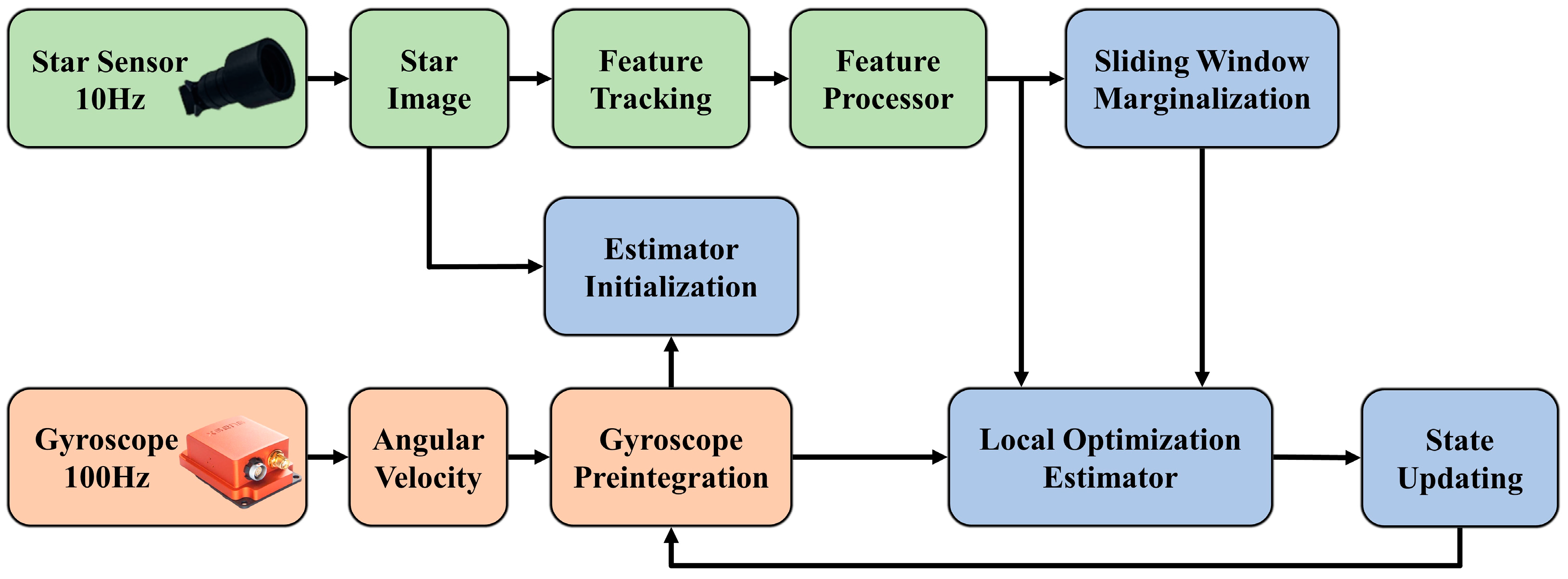
The structure of proposed tightly coupled visual–inertial fusion method is depicted in Figure 1. The system starts by preprocessing the raw measurements of the two sensors, where stars are extracted as features and tracked. The gyroscope measurements between two consecutive frames are pre-integrated simultaneously. During the initialization procedure, a loosely coupled approach between vision and the gyroscope is employed. At first, the initial attitude of every frame in the sliding window is determined by using star identification through the star sensor. Later, this information is used to align with the pre-integration of the gyroscope to initialize the bias. The nonlinear optimization estimator jointly optimizes the visual reprojection errors, inertial pre-integration errors, absolute attitude error, and marginalized information constructed from all the keyframes in the sliding window to achieve the optimal state estimation.

We employ the following notation throughout this work:${(·)}^w$ denotes the world frame and for spacecraft it is also consistent with International Celestial Reference System (ICRS). ${(·)}^b$ denotes the body frame, which is defined to be the same as the gyroscope frame. Thus, the attitude of the spacecraft in the inertial frame can be expressed as $R_b^w$. We consider ${(·)}^c$ as the star sensor frame; there exists a rotation matrix $R_c^b$ from the star sensor frame to gyroscope frame. $b_k$ is the body frame of k-th image. Furthermore, we also represent the rotation using the Hamilton quaternions, and the attitude kinematics model is $q_{i+1}{=q}_{\mathrm{i}}\otimes \delta q$. $\otimes$ represents the multiplication operation between two quaternions. $\left(\widehat{·}\right)$ is considered as the actual noisy measurement or estimation of a certain quantity.

The remaining sections of this paper are organized as follows: Section 3 outlines the preprocessing of raw measurements from the sensors, Section 4 details the nonlinear estimator initialization process, and next, Section 5 provides comprehensive constraint information about the nonlinear estimator. Experiment results are shown and discussed in Section 6. Section 7 concludes with a summary and discussion of our work.

3. Measurement Preprocessing

From this section onwards, a comprehensive introduction to the visual–inertial tightly coupled fusion scheme is provided, which comprises three primary elements. Prior to introducing each component separately, it is assumed that the camera has completed intrinsic parameters calibration, which includes focal length, principal point, and optical lens distortion, resulting in known intrinsic parameter matrix. Moreover, the extrinsic parameters between the camera and the gyroscope were previously determined, and star catalog errors are neglected. Additionally, we assume that the trigger signal was aligned, disregarding the measurement delay between the two sensors.

3.1. Gyroscope Pre-Integration

The raw measurement of gyroscope is given by the following:

$$\widehat{\mathit{\omega }}=\mathit{\omega }+\mathit{b}+n_g$$

(1)

where $\mathit{\omega }$ denotes true value without noise of angular velocity. b denotes a slowly varying term about constant bias, and it consists of two parts: the constant part ${\mathit{b}}_f$ and the random part ${\mathit{b}}_{\omega }$, which is also called random walk. It can be described as the Wiener process: $\dot{ {\mathit{b}}_{\omega }}{=n}_{\omega }{,n}_{\omega }{~N(0,\sigma }_{\omega }^2)$, and its unit in continuous form is ${\mathrm{rad}/\mathrm{s}}^2/\sqrt{\mathrm{Hz}}$. $n_g$ is an additive Gaussian white noise term, $n_g{~N(0,\sigma }_g^2)$; its unit in continuous form is $\mathrm{rad}/\mathrm{s}/\sqrt{\mathrm{Hz}}$. Both of their units in discrete form are $\mathrm{rad}/\mathrm{s}$.

Given two consecutive frames, denoted as $b_k$ and $b_{k+1}$, the attitude in the world frame can be propagated by using the gyroscope measurements during the time interval ${[t}_k{,t}_{k+1}]$, which can be used as the initial state of the $b_{k+1}$ frame.

$${\mathit{q}}_{b_{k+1}}^w={\mathit{q}}_{b_k}^w\otimes {\displaystyle {\int }_{t\in \left[k,k+1\right]}\frac{1}{2}\Omega \left({\widehat{\mathit{\omega }}}_t-{\mathit{b}}_t\right)}{\mathit{q}}_t^{b_k}dt$$

(2)

where

$$\Omega \left(\mathit{\omega }\right)=\left[\begin{array}{cc}-{\mathit{\omega }}^{\wedge }& \mathit{\omega }\\ -{\mathit{\omega }}^T& 0\end{array}\right],{\mathit{\omega }}^{\wedge }=\left[\begin{array}{ccc}0& -{\omega }_z& {\omega }_y\\ {\omega }_z& 0& -{\omega }_x\\ -{\omega }_y& {\omega }_x& 0\end{array}\right]$$

(3)

It can be seen that current attitude depends on the previous states (attitude and bias). However, the optimization method seeks to optimize all states over a period of time, which can lead to redundant calculations. Therefore, the primary motivation for pre-integration is to separate the absolute attitude from the state variables.

$${\mathit{\beta }}_{b_{k+1}}^{b_k}={\mathit{q}}_{b_k}^{w-1}\otimes {\mathit{q}}_{b_{k+1}}^w={\displaystyle {\int }_{t\in \left[k,k+1\right]}\frac{1}{2}\Omega \left({\widehat{\mathit{\omega }}}_t-{\mathit{b}}_t\right)}{\mathit{q}}_t^{b_k}dt$$

(4)

with $b_k$ serving as the reference frame, the pre-integration term Equation (4) can be derived solely from gyroscope measurements. However, the bias is still the state to be optimized in the estimator; it need to be separated from the pre-integration term from the bias error. To simplify the mathematical formulation, the following assumptions are made: (1) The bias value ${\mathit{b}}_t$ at each moment is assumed to be constant and remains fixed throughout the entire pre-integration calculation process. (2) When the bias value changes, it is approximately corrected using a linear model during pre-integration. (3) Only the first-order linear model for bias is retained, while higher-order terms are discarded. Therefore, we have the following:

$${\mathit{\beta }}_{b_{k+1}}^{b_k}\approx {\widehat{\mathit{\beta }}}_{b_{k+1}}^{b_k}\otimes \left[\begin{array}{c}1\\ {\displaystyle \frac{1}{2}}{\mathit{J}}_b^{\beta }\delta \mathit{b}\end{array}\right]$$

(5)

where ${\mathit{J}}_b^{\beta }=\partial {\mathit{\beta }}_{b_{k+1}}^{b_k}/\partial \mathit{b}$ denotes the Jacobian matrix of attitude with respect to bias. ${\widehat{\mathit{\beta }}}_{b_{k+1}}^{b_k}$ denotes the attitude increment between two consecutive frames without bias error. The derivation details of continuous-time linearized dynamics of error terms and noise covariance matrix can be found in the paper [35], which is also similar to ESKF [17].

3.2. Visual Preprocessing

Since stars can be regarded as sources at infinity, the imaging model of THE star sensor can be considered to satisfy the pinhole projection model. Consider $\mathit{w}$ as a star vector in the inertial frame; its right ascension and declination are $\alpha$ and $\delta$, respectively.

$$w=\left[\begin{array}{c}\cos \alpha \cos \delta \\ \sin \alpha \cos \delta \\ \sin \delta \end{array}\right]$$

(6)

Assume that the x-axis is the camera’s optical axis. The projected point p in the image frame can be expressed as given:

$$\mathit{p}=\left[\begin{array}{c}1\\ u\\ v\end{array}\right]=\left[\begin{array}{ccc}1& 0& 0\\ c_x& f_x& 0\\ c_y& 0& f_y\end{array}\right]\left[\begin{array}{c}1\\ -Y/X\\ -Z/X\end{array}\right]=\mathit{K}\mathit{P}=\mathit{K}{\mathit{R}}_w^c\mathit{w}$$

(7)

where $(u,v)$ represent pixel values. K denotes the camera intrinsics matrix, and f represents the pixel-level focal length, measured in pixels. Here, it is assumed that the horizontal and vertical dimensions of the pixel are the same; ${(u}_0{,v}_0)$ represent the principal point position. P is the vector in the camera frame, which is calculated by star vector w and attitude matrix ${\mathit{R}}_c^w$ between the inertial and camera frame.

Given two or more star vectors, there are two methods for solving the attitude matrix ${\mathit{R}}_c^w$. The first method involves linear algebra techniques such as SVD and QUEST [36]. The second method employs nonlinear optimization, which is similar to bundle adjustment (BA).

When a new frame of image is obtained, the centroid method is used to extract stars. After completing the star identification for the first image, two strategies were employed to track and match the features. The Lucas–Kanade (LK) optical flow method [37] was used when the gyroscope had not been corrected for bias. After the bias correction, feature tracking was performed using the dynamics propagation model.

Between two sequential frames, for each star feature, the dynamics propagation model can be easily obtained by using the Equations (2) and (7) as follows:

$$\{\begin{array}{c}{u}_{i+1}={\displaystyle \frac{u_i+v_i{\omega }_x\Delta t+f{\omega }_z\Delta t}{\left(-u_i{\omega }_z\Delta t+v_i{\omega }_y\Delta t\right)/f+1}}\\ v_{i+1}={\displaystyle \frac{v_i-u_i{\omega }_x\Delta t-f{\omega }_y\Delta t}{\left(-u_i{\omega }_z\Delta t+v_i{\omega }_y\Delta t\right)/f+1}}\end{array}$$

(8)

where the pairs of ${(u}_i{,v}_i)$ and ${(u}_{i+1}{,v}_{i+1})$ denote pixel coordinates of the same star under continuous gyroscope sampling. $\left({\omega }_x{,\omega }_y{,\omega }_z\right)$ denote the angular velocity of the three axes, in units of rad/s, and f represents the focal length.

4. Estimator Initialization

The gyroscope constant bias varies each time it is started up, and it is not a fixed value. The ground calibration results only represent statistical characteristics during a specific period in a particular environment. Furthermore, environmental factors such as the temperature and mechanical vibration can affect the random walk. Therefore, it is necessary to initialize the gyroscope bias to obtain a precise value to enhance optimization [38].

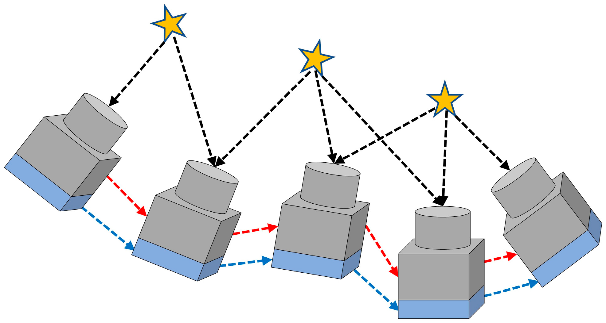
In this paper, we employ attitude alignment approach to estimate the initial gyroscope bias. As spacecraft move slowly and steadily during star identification, the star sensor provides very accurate attitude measurements. Therefore, as depicted in Figure 2, aligning the visual and inertial relative attitude among all image frames within the initial sliding window can effectively eliminate bias. Furthermore, to expedite the star searching process, we employed the LK optical flow method to track identified stars after completing the initial star identification for the first image frame.

Assuming there are two consecutive frames $b_k$ and $b_{k+1}$ in the sliding window $\mathit{S}$, we have solved the attitude ${\mathit{q}}_{b_k}^w$ and ${\mathit{q}}_{b_{k+1}}^w$ from star sensor and the corresponding pre-integration ${\mathit{\beta }}_{b_{k+1}}^{b_k}$ from the gyroscope. If the gyroscope has no bias, the relative attitude determined by the two sensors should be precisely identical. A cost function can be obtained as follows:

$$\underset{\delta b}{min}{\displaystyle \sum _{k=0}^{S-1}{\Vert {\left({\mathit{\beta }}_{b_{k+1}}^{b_k}\right)}^{-1}\otimes {\left({\mathit{q}}_{b_k}^w\right)}^{-1}\otimes {\mathit{q}}_{b_{k+1}}^w\Vert }^2}$$

(9)

According to Equation (5), pre-integration can be linearized with bias, Moreover, since the minimum value of the cost function is the unit quaternion, and we only consider the imaginary part of quaternions, it can be expressed as follows:

$${\displaystyle \prod _{k=0}^{S-1}{\mathit{J}}_b^{\beta }\delta \mathit{b}}={\displaystyle \prod _{k=0}^{S-1}2{\left({\left({\widehat{\mathit{\beta }}}_{b_{k+1}}^{b_k}\right)}^{-1}\otimes {\left({\mathit{q}}_{b_k}^w\right)}^{-1}\otimes {\mathit{q}}_{b_{k+1}}^w\right)}_{vec}}$$

(10)

where ${(·)}_{\mathit{vec}}$ takes the imaginary part of quaternions. Then, we perform Cholesky decomposition on the above equation. After solving for the gyroscope bias, it is necessary to recompute all pre-integration terms in a sliding window. A suitable initial bias will reduce the impact of the first sliding window’s attitude on subsequent attitude estimations.

5. Nonlinear Optimization Estimator

After initialization of the estimator, the algorithm primarily utilizes batch optimization methods to achieve visual–inertial tightly coupled attitude estimation for spacecraft in high-dynamic scenarios. This method provides optimal estimation of attitude and gyroscope bias. Additionally, a sliding window is introduced to limit the state size and meet real-time requirements. The sliding window comprises all the information regarding the frames, including image information and gyroscope pre-integration. Only frames with sufficient feature displacement in the image are considered as keyframes. This system ensures that there are not too many common view features between frames, which could result in an overly dense H matrix during least-squares optimization. Here, the H matrix is the square of the first-order Jacobian matrix, which serves as an approximation of the second-order Hessian matrix used in the Gauss-Newton method. 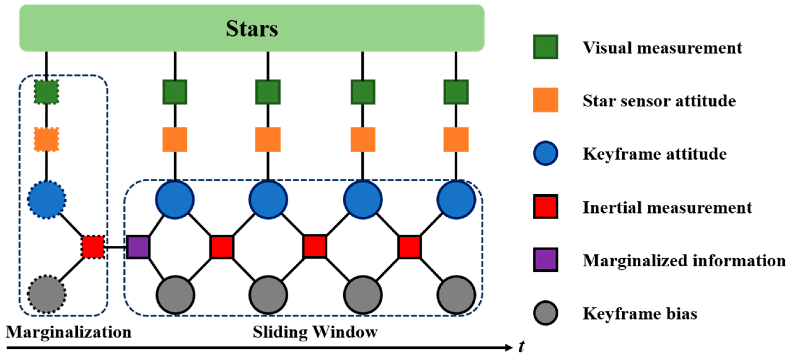Figure 3 illustrates the operational principle of the nonlinear optimization estimator when the latest image frame serves as a keyframe.

For the sake of convenience in notation, the state ${\mathit{x}}_k$ of the ${\mathit{b}}_k$ frame includes the attitude in the world frame ${\mathit{R}}_{b_k}^w\left({\mathit{q}}_{b_k}^w\right)$ and the bias ${\mathit{b}}_k$ in the body frame. We consider N+1 frames in the sliding window, starting at 0 and ending at N. Here, the time index N always refers to the latest image, and the state vector to be estimated is defined as follows:

$$\mathit{X}=\left[x_{0:N-1},x_N\right]$$

(11)

The tightly coupled problem of visual–inertial fusion can be expressed as a joint optimization of a cost function comprising errors from all sensors’ measurements:

$$\underset{X}{min}\left\{{\Vert e_p\left(\mathit{X}\right)\Vert }^2+{\displaystyle \sum _{k=0}^{S-1}{\Vert e_{b_{k+1}}^{b_k}\left(\mathit{X}\right)\Vert }_{W_{b_{k+1}}^{b_k}}^2}+{\displaystyle \sum _{i,j=0}^S{\displaystyle \sum _{l\in \zeta \left(i,j\right)}{\Vert e_l^{c_{ij}}\left(\mathit{X}\right)\Vert }_{W_l^{c_{ij}}}^2}}+{\displaystyle \sum _{k=0}^S{\displaystyle \sum _{l\in b_k}{\Vert e_l^{b_k}\left(\mathit{X}\right)\Vert }_{W_l^{c_k}}^2}}\right\}$$

(12)

where $e_p\left(\mathit{X}\right)$ denotes the marginalized information. $e_{b_{k+1}}^{b_k}\left(\mathit{X}\right)$, $e_l^{c_{ij}}\left(\mathit{X}\right)$, and $e_l^{c_k}\left(\mathit{X}\right)$ denote the error for inertial, visual, and absolute attitude measurement, respectively. Similarly, ${\mathit{W}}_{b_{k+1}}^{b_k}$,${\mathit{W}}_{\mathrm{l}}^{c_{ij}}$, and ${\mathit{W}}_l^{c_k}$ denote their corresponding information matrices. The indexes of features visible in the i-th frame and the j-th camera are written as the set $\zeta (i,j)$. Since the observation model’s noise is assumed to follow a Gaussian distribution, the least-squares method actually optimizes the error expressed as the Mahalanobis distance. The Mahalanobis distance is a weighted Euclidean distance by the information matrix. Hence, the information matrix is related to the noise term and is the inverse of the noise covariance matrix. The information matrix can be seen as the weight of the error term. The larger the information matrix, the smaller the observation noise, and the more reliable the measurements from the sensor.

For solving the least-squares problem utilizing the nonlinear Gauss–Newton method, it is possible to express each error term as follows:

$$e\left(\mathit{X}\right)=e\left(\mathit{X}+{\mathit{J}}_X\delta \mathit{X}\right)$$

(13)

where ${\mathit{J}}_{\mathit{X}}$ is the Jacobian matrix of errors with respect to the state variables. $\delta \mathit{X}$ is a small perturbation in the state variables.

In the following, we introduce individual measurement errors from various sensors.

5.1. Inertial Measurement Error

The gyroscope measurement errors denote the bias error between successive frames and the subsequent alteration in attitude due to this bias error. These errors reflect the discrepancy between the observed and estimated values. Therefore, we can define the gyroscope measurement error $e_{b_{k+1}}^{b_k}$ between any two consecutive frames within a sliding window $\mathit{S}$ as follows:

$$e_{b_{k+1}}^{b_k}\left(\mathit{X}\right)=\left[\begin{array}{c}\delta {\mathit{\theta }}_{b_{k+1}}^{b_k}\\ \delta {\mathit{b}}_{b_{k+1}}^{b_k}\end{array}\right]=\left[\begin{array}{c}2{\left({\left({\widehat{\mathit{\beta }}}_{b_{k+1}}^{b_k}\right)}^{-1}\otimes {\left({\mathit{q}}_{b_k}^w\right)}^{-1}\otimes {\mathit{q}}_{b_{k+1}}^w\right)}_{vec}\\ {\mathit{b}}_{k+1}-{\mathit{b}}_k\end{array}\right]$$

(14)

where ${\widehat{\mathit{\beta }}}_{b_{k+1}}^{b_k}$ denotes the attitude increment without bias change, which was discussed in the gyroscope pre-integration section. It can be seen that each gyroscope measurement error term is only related to frame $b_k$ and $b_{k+1}$ and is independent of other frames within the sliding window. This means that the partial derivative of the error term with respect to unrelated state variables in the Jacobian matrix is 0.

$$\begin{array}{l}{\displaystyle \frac{\partial e_{b_{k+1}}^{b_k}}{\partial \left[{\mathit{q}}_{b_k}^w,{\mathit{b}}_k\right]}}=\left[\begin{array}{cc}\left[{\mathbf{0}}_{3\times 1},-{\left(ℒ\left({\left({\mathit{q}}_{b_{k+1}}^w\right)}^{-1}\otimes {\mathit{q}}_{b_k}^w\right)ℛ\left({\widehat{\mathit{\beta }}}_{b_{k+1}}^{b_k}\right)\right)}_{bot}\right]& -{\left(ℒ\left({\left({\mathit{q}}_{b_{k+1}}^w\right)}^{-1}\otimes {\mathit{q}}_{b_k}^w\otimes {\widehat{\mathit{\beta }}}_{b_{k+1}}^{b_k}\right)\right)}_{bot}{\mathit{J}}_{b_k}^{\beta }\\ {\mathbf{0}}_{3\times 4}& -{\mathit{I}}_{3\times 3}\end{array}\right]\\ {\displaystyle \frac{\partial e_{b_{k+1}}^{b_k}}{\partial \left[{\mathit{q}}_{b_{k+1}}^w,{\mathit{b}}_{k+1}\right]}}=\left[\begin{array}{cc}\left[{\mathbf{0}}_{3\times 1},{\left(ℒ\left({\left({\widehat{\mathit{\beta }}}_{b_{k+1}}^{b_k}\right)}^{-1}\otimes {\left({\mathit{q}}_{b_k}^w\right)}^{-1}\otimes {\mathit{q}}_{b_{k+1}}^w\right)\right)}_{bot}\right]& {\mathbf{0}}_{3\times 3}\\ {\mathbf{0}}_{3\times 4}& {\mathit{I}}_{3\times 3}\end{array}\right]\end{array}$$

(15)

where

$$ℒ\left(\mathit{q}\right)=\left[\begin{array}{cc}s& -{\mathit{v}}^T\\ \mathit{v}& s\mathit{I}+{\mathit{v}}^{\wedge }\end{array}\right],ℛ\left(\mathit{q}\right)=\left[\begin{array}{cc}s& -{\mathit{v}}^T\\ \mathit{v}& s\mathit{I}-{\mathit{v}}^{\wedge }\end{array}\right]$$

(16)

$\mathit{q}=[s,\mathit{v}]$; s represents the real part, and v represents the vector part. ${(·)}_{\mathit{bot}}$ extracts the lower-right $3\times 3$ block of the given matrix. The derivation of the Jacobian matrix is given in the Supplementary Materials.

5.2. Visual Reprojection Error

In a pinhole camera model, the reprojection error on the image plane is typically defined. Figure 4 illustrates a scenario where there is a point l in space, which is projected onto the image planes $c_i$ and $c_j$, resulting in pixel coordinates $p_1$ and $p_2$, respectively. The predicted pixel location on $c_j$, denoted as ${\widehat{p}}_2$, is obtained by rotating $p_1$ with ${\mathit{R}}_{c_i}^{c_j}$. In this case, the reprojection error is the difference between the predicted pixel coordinates ${\widehat{p}}_2$ and the corresponding observed pixel coordinates $p_2$.

We consider that two distinct image planes, $c_i$ and $c_j$, share a common observed feature l. The visual error of this feature can be defined as follows:

$$e_l^{c_{ij}}\left(\mathit{X}\right)=\left[\begin{array}{l}{\widehat{u}}_l^{c_j}-u_l^{c_j}\\ {\widehat{v}}_l^{c_j}-v_l^{c_j}\end{array}\right]$$

(17)

where $(u_l^{c_j},v_l^{c_j})$ and $({\widehat{u}}_l^{c_j},{\widehat{v}}_l^{c_j})$ denote the observed and predicted pixel coordinates of l in camera plane $c_j$, respectively. The visual preprocessing section discussed the utilization of ${\widehat{\mathit{P}}}_l^{c_j}=\left({\widehat{x}}_l^{c_j},{\widehat{y}}_l^{c_j},{\widehat{z}}_l^{c_j}\right)$ to signify feature vector under the camera frame. So, it can be calculated in the following way:

$${\widehat{\mathit{P}}}_l^{c_j}={\mathit{R}}_b^c{\mathit{R}}_w^{b_j}{\mathit{R}}_{b_i}^w{\mathit{R}}_c^b{\mathit{P}}_l^{c_i}$$

(18)

${\mathit{P}}_l^{c_i}{=(x}_l^{c_i}{,y}_l^{c_i}{,z}_l^{c_i})$ is the observed vector of l under the camera frame $c_i$. Therefore, we can establish two-frame attitude constraints through visual errors, which are different from inertial constraints that need to be between adjacent frames. These constraints are connected by a shared visual feature across several frames.

The derivative of the state variables follows the chain rule of differentiation and is taken with respect to the attitude in the world frame. This allows the perturbation rotation to be expressed in the form of right multiplication. It is noteworthy that we defined the x-axis of the camera as its optical axis. The calculation method is as follows:

$${\displaystyle \frac{\partial e_l^{c_{ij}}}{\partial {\mathit{R}}_{b_i}^w}}={\displaystyle \frac{\partial e_l^{c_{ij}}}{\partial {\widehat{\mathit{P}}}_l^{c_j}}}{\displaystyle \frac{\partial {\widehat{\mathit{P}}}_l^{c_j}}{\partial {\mathit{R}}_{b_i}^w}}$$

(19)

So, the first term on the right-hand side of the equation represents the derivative of the error term with respect to the three dimensions of ${\widehat{\mathit{P}}}_l^{c_j}$. According to Equation (7), it is not difficult to deduce:

$${\displaystyle \frac{\partial e_l^{c_{ij}}}{\partial {\widehat{\mathit{P}}}_l^{c_j}}}=\left[\begin{array}{c}\begin{array}{ccc}{\displaystyle \frac{{\widehat{y}}_l^{c_j}}{{{\widehat{x}}_l^{c_j}}^2}}& -{\displaystyle \frac{1}{{\widehat{x}}_l^{c_j}}}& 0\end{array}\\ \begin{array}{ccc}{\displaystyle \frac{{\widehat{z}}_l^{c_j}}{{{\widehat{x}}_l^{c_j}}^2}}& 0& -{\displaystyle \frac{1}{{\widehat{x}}_l^{c_j}}}\end{array}\end{array}\right]$$

(20)

The second term in the equation is obtained directly by taking the derivative of Equation (18) with respect to the rotation matrix. Similar to solving for inertial measurement errors, it is also achieved by applying small perturbations to the relevant rotation matrices. Therefore, we obtain the following:

$${\displaystyle \frac{\partial {\widehat{\mathit{P}}}_l^{c_j}}{\partial {\mathit{R}}_{b_i}^w}}=-{\mathit{R}}_b^c{\mathit{R}}_w^{b_j}{\mathit{R}}_{b_i}^w{\left({\mathit{R}}_c^b{\mathit{P}}_l^{c_i}\right)}^{\wedge }$$

(21)

Using the same method, we can obtain the derivative of both variables ${\mathit{R}}_{b_j}^w$. The process of derivation is included in the Supplementary Materials.

$${\displaystyle \frac{\partial {\widehat{\mathit{P}}}_l^{c_j}}{\partial {\mathit{R}}_{b_j}^w}}={\mathit{R}}_b^c{\left({\mathit{R}}_w^{b_j}{\mathit{R}}_{b_i}^w{\mathit{R}}_c^b{\mathit{P}}_l^{c_i}\right)}^{\wedge }$$

(22)

5.3. Absolute Attitude Error

The above two error terms describe the relative attitude constraints between two image frames, thus lacking absolute attitude as a reference baseline. However, the state propagation relies on the dynamics of the gyroscope attitude equation, which leads to accumulated errors over longer optimization cycles and cannot be easily resolved on its own. While SLAM systems rely on loop closure detection to identify repeated environmental features in the map and then correct previous localization and map construction based on these repeated features to reduce the impact of accumulated errors, this approach is not practical for spacecraft. To address this issue, a new error term is proposed, which aims to minimize the accumulated errors due to optimization by using absolute attitude calculated from the star sensor. We refer to this as absolute attitude error. The construction method of this constraint is similar to visual reprojection error, ensuring the maximum reduction of potential errors in the optimization system and providing a more accurate assessment of the absolute accuracy of sensor measurements.

As demonstrated in Figure 5, $c_k$ is a frame within the sliding window S. In the case of a feature, the observed pixel from the image is $p_l$, whereas the predicted pixel using Equation (8) is ${p^{\prime }}_l$. Due to various factors, such as extraction errors and gyroscope bias, a slight rotation $\mathit{Exp}(\varphi )$ takes place to align $p_l$ and ${p^{\prime }}_l$, where Exp(·) is the exponential map, which can convert a vector belonging to the Lie algebra into a rotation matrix that corresponds to the Lie group.

Similar to Equation (17), the absolute attitude error can be defined as follows:

$$e_l^{c_k}\left(\mathit{X}\right)=\left[\begin{array}{l}{\widehat{u}}_l^{c_k}-u_l^{c_k}\\ {\widehat{v}}_l^{c_k}-v_l^{c_k}\end{array}\right]$$

(23)

The transformation relationship of the feature vector in the camera frame can be determined through utilization of the equation presented below:

$${\widehat{\mathit{P}}}_l^{c_k}={\mathit{R}}_w^{c_k}{\mathit{R}}_{b_k}^w{\mathit{R}}_c^b{{\mathit{P}}^{\prime }}_l$$

(24)

where ${\mathit{R}}_{c_k}^w$ and ${\mathit{R}}_{b_k}^w$ denote the attitude calculated by the star sensor and gyroscope, respectively. It is worth noting that the states to be optimized are represented by ${\mathit{R}}_{b_k}^w$, while ${\mathit{R}}_{c_k}^w$ is the considered constant. Here, we will not reiterate the process of differentiating with respect to variables as outlined in Equation (19).

5.4. Marginalized Information

As the estimation time increases, the size of the states to be estimated will continue to grow, leading to a sharp increase in computational complexity and a decrease in algorithm efficiency. Typically, a sliding window based on keyframes is used to control the size of the states to be optimized, with optimization limited to a subset of keyframes from past moments and the current frame, as shown in Figure 3. Discarding past states requires the application of marginalization techniques. Marginalization is a technique that discards the oldest keyframe states within the sliding window while retaining their prior information to constrain the current frame.

As shown in Figure 6, this approach employs two marginalization strategies based on whether the newly acquired image frame is a keyframe. Firstly, if the image frame is a keyframe, then the oldest keyframe within the sliding window is marginalized. Gyroscope states and features with almost no co-visibility with other keyframes are marginalized, transforming into prior information $e_p\left(\mathit{X}\right)$ added to the overall objective function. This is because star features are very sparse, and there may be multiple co-visible features between keyframes. Marginalizing all measurements of the oldest keyframe would result in an overly dense H matrix, making optimization solving difficult. Secondly, if the image frame is not a keyframe, then the measurements of the newest keyframe within the sliding window are directly replaced with the new measurements. However, gyroscope measurements still need to be retained to ensure pre-integration consistency. The process of marginalization is performed utilizing the Schur complement, and readers can refer to the paper [39] for its details.

6. Experiments and Results

In this section, simulation and experiments are provided to validate the reliability of the proposed method. All the work was implemented using C++ code and optimized using the Google Ceres optimizer [40] and Levenberg–Marquardt algorithm to optimize the aforementioned objective function.

6.1. Simulations

To facilitate better comparison of results, an EKF algorithm [41] was implemented using C++ code. EKF is currently the most widely used attitude estimation algorithm for spacecraft because spacecraft attitude estimation typically involves weakly nonlinear systems. Additionally, EKF has low computational complexity and performs well in real-time applications. Both methods use the same sensor parameters.

Table 1. Parameters of visual–inertial combination system.

Camera Parameters		Gyroscope Parameters
Focal Length	15 mm	Bias Error	$0.05°/\mathrm{s}$
Image Size	1024 × 1024	Random Walk	$0.0005°/\mathrm{s}$
Field of View	20°	White Noise	$0.005°/\mathrm{s}$
Exposure Time	100 ms	Output Rate	100 Hz

lists the specific parameters for the star sensor and gyroscope, where gyroscope noise parameters are in continuous-time form. A star chart was constructed in Matlab 2016 using stars from the Smithsonian Observatory Catalogue (SAO) with brightness exceeding 6Mv for star chart simulation. The camera model used a pinhole imaging model and was defocused.

A sinusoidal curve motion was applied to the yaw, pitch, and roll axes’ angular velocities, and 1000 star images were continuously simulated, as shown in Figure 7. The proposed method uses a sliding window that retains historical information from the past 12 keyframes. The first 12 images within the sliding window were considered keyframes and used for estimator initialization. Subsequently, a new keyframe was established every eight images.

Figure 8 illustrates the attitude and bias estimation results obtained using the proposed optimization method and the EKF algorithm under a standard deviation of 0.3 pixels for star position error. Subfigures (a)–(c) show the attitude estimation errors for the yaw, pitch, and roll axes, while subfigures (d)–(f) display the bias estimation for all three axes. Both the attitude and bias estimation results of the proposed method outperformed those of the EKF algorithm. During the initial stages of optimization, there may be transient erroneous estimates due to the gyroscope not yet completing initialization within the first sliding window. However, once initialization is completed, it provides good initial bias values to accelerate the convergence of the algorithm.

Star position error is the primary factor affecting the accuracy of star sensor attitude measurements, with estimation accuracy decreasing as star point position error increases. It is important to note that the roll angle is most affected. This is determined by the nature of the camera itself, as pixel movements of the camera are insensitive to rotations about the line of sight (the optical axis perpendicular to the target surface). Conversely, roll angle errors are highly sensitive to pixel errors. Even small position errors can amplify roll angle errors. Therefore, under the same position error, the estimation error of the roll angle by the star sensor may be nearly 10 times larger than that of the other two axes.

6.2. The Robustness of Attitude Estimation

The accuracy of attitude estimation is significantly influenced by the error in star positions. To assess the algorithm’s performance under different star sensor position errors, six sets of noise ranging from 0.1 to 0.6 pixels were applied. Each set was independently repeated ten times, and the results were averaged. Gyroscope parameters remained constant. A comparison was made with the results obtained from the EKF algorithm and directly computed by the star sensor.

Table 2. Standard deviation of three-axis attitude error under different position errors.

	Star Sensor			EKF			Our Approach
Pixel Error	${\mathit{\sigma }}_{\mathit{yaw}}(″)$	${\mathit{\sigma }}_{\mathit{pitch}}(″)$	${\mathit{\sigma }}_{\mathit{roll}}(″)$	${\mathit{\sigma }}_{\mathit{yaw}}(″)$	${\mathit{\sigma }}_{\mathit{pitch}}(″)$	${\mathit{\sigma }}_{\mathit{roll}}(″)$	${\mathit{\sigma }}_{\mathit{yaw}}(″)$	${\mathit{\sigma }}_{\mathit{pitch}}(″)$	${\mathit{\sigma }}_{\mathit{roll}}(″)$
0.1	1.8	1.7	14	1.3	1.2	10.5	1.1	1.1	6.7
0.2	3.6	3.4	27.2	2.5	2.3	20.6	1.9	2	12.9
0.3	5.4	5.4	41.4	3.6	3.5	33.7	2.9	2.8	18.8
0.4	7	6.8	54.8	4.8	4.6	43.8	3.7	3.5	28.4
0.5	8.5	8.3	65.7	6.1	5.8	47.4	4.6	4.2	32.9
0.6	10.4	10.3	83.7	7	7.1	62.4	5.3	5.3	45

presents the standard deviation of three-axis attitude errors under different star position errors. As shown in Figure 9, the three-axis attitude estimation almost linearly increases with the increase in star position error. This is because observation noise directly affects two constraints in the cost function, namely camera visual reprojection error and absolute attitude error, ultimately leading to decreased solution accuracy. Additionally, observation noise also affects the estimation of gyroscope bias, ultimately impacting gyroscope pre-integration constraints. As illustrated in Figure 8, the estimation error of the roll axis is significantly higher than that of the other two axes. However, in high-dynamic scenes, the proposed optimization method significantly improves the three-axis estimation accuracy, with all three axes showing an increase of nearly 50% compared to the attitude solved by the star sensor only.

Gyroscope measurement noise is also a crucial factor influencing attitude estimation. To test the impact of gyroscope accuracy on the performance of the proposed method, different levels of measurement noise were set. The standard deviations in continuous form were sequentially set to ${1\times 10}^{-3}°/\sqrt{\mathrm{s}}$, ${1\times 10}^{-4}°/\sqrt{\mathrm{s}}$, ${1\times 10}^{-5}°/\sqrt{\mathrm{s}}$, and ${1\times 10}^{-6}°/\sqrt{\mathrm{s}}$. The star position error was maintained at 0.3 pixels, with constant bias at ${1\times 10}^{-3}°/\mathrm{s}$ and random walk at ${5\times 10}^{-5}°/\mathrm{s}\sqrt{\mathrm{s}}$. Each set was independently repeated ten times, and the final results were averaged. The simulation results are shown in Figure 10, and the numerical results are presented in

Table 3. Results of three-axis attitude error.

$\mathbf{Noise}(°/\sqrt{\mathbf{s}}$)	${1\times 10}^{-6}$	${1\times 10}^{-5}$	${1\times 10}^{-4}$	${1\times 10}^{-3}$
${\sigma }_{\mathit{yaw}}(″)$	2.80	2.83	2.91	3.58
${\sigma }_{\mathit{pitch}}(″)$	2.68	2.72	2.76	3.53
${\sigma }_{\mathit{roll}}(″)$	18.38	18.62	18.76	21.17

.

It can be observed that when the gyroscope measurement noise is less than ${1\times 10}^{-4}°/\sqrt{\mathrm{s}}$, the three-axis estimation accuracy hardly improves, indicating that the estimation is mainly affected by star position error at this level of noise. Moreover, when the noise level increases by ten times, the accuracy of the three axes does not significantly decrease, suggesting that the proposed algorithm can adapt to higher noise levels.

6.3. The Robustness of Bias Estimation

The gyroscope’s constant bias is not a fixed value; it varies each time it is powered on and used. Offline calibration values only reflect the statistical characteristics over a period of time in a specific working environment. Additionally, bias undergoes slow changes during usage due to environmental factors such as temperature, described as the angular rate random walk using Wiener processes. Therefore, both the constant bias and angular rate random walk are crucial parameters influencing gyroscope bias estimation. Similarly, under the condition of keeping other sensor parameters unchanged, multiple sets of different constant biases and angular rate random walks were configured to evaluate the accuracy of the proposed algorithm in estimating gyroscope bias.

Figure 11 illustrates the estimation results of three sets of gyroscope constant bias, with parameters in subfigures (a)–(c) set to ${1\times 10}^{-3}°/\mathrm{s}$, ${1\times 10}^{-2}°/\mathrm{s}$, and ${1\times 10}^{-1}°/\mathrm{s}$, respectively. It is evident that no prior calibration values are required, and the gyroscope can obtain good initial bias values through a simple initialization process. Additionally, from the results, it can be observed that the presence of constant bias does not affect the accuracy of bias estimation due to initialization. Figure 12 presents the estimation results of bias under three different levels of random walk, with parameters in subfigures (a)–(c) set to ${5\times 10}^{-5}°/\mathrm{s}\sqrt{\mathrm{s}}$, ${5\times 10}^{-4}°/\mathrm{s}\sqrt{\mathrm{s}}$, and ${1\times 10}^{-3}°/\mathrm{s}\sqrt{\mathrm{s}}$, respectively. From the results, it can be seen that even under conditions of significant random walk, the proposed algorithm can dynamically estimate the bias. Although there is a certain lag in estimation during periods of rapid change; the bias can be accurately estimated once it stabilizes.

6.4. The Outlier Test for the Star Sensor

Scenarios such as stray light and extreme conditions can cause temporary spatial disorientation and anomalies in star sensor measurements. Traditional filter methods lack the capability to update the state with measurements, relying solely on the gyroscope for state propagation. In contrast, the proposed optimization method seeks the optimal state estimation over a period of time. When visual observations are lacking, it constrains the current estimation based on information retained from past image frames and the current gyroscope measurements until new valid observations are obtained. Additionally, upon regaining valid measurements, the star sensor only needs to quickly identify stars based on the current attitude, without the need for reidentification across the entire celestial sphere or large local sky areas. To address the extreme scenarios described above, corresponding simulation experiments were designed. The attitude and bias estimation results are shown in Figure 13. Even when star sensor measurement data are unavailable for up to 10 s, i.e., no input from 100 star images, the proposed method (blue line) maintains good attitude estimation across all three axes. Once new valid observation information is obtained, the star sensor quickly resumes output (red line).

Table 4. Estimation error of three-axis attitudes during different periods of image information loss.

Time (s)	1	5	7	10
${\sigma }_{\mathit{yaw}}(″)$	2.9	2.9	2.8	2.9
${\sigma }_{\mathit{pitch}}(″)$	2.8	2.8	2.8	2.8
${\sigma }_{\mathit{roll}}(″)$	18.8	20.4	21.1	21.4

shows the estimation accuracy of the three-axis attitude of the star sensor under different durations of spatial disorientation. From the results, even when image loss occurs for up to 10 s, the attitude estimation accuracy of the yaw and pitch axes remains unaffected thanks to the accuracy of the estimation of the two-axis bias. Although the accuracy of the roll axis is slightly reduced, with an average decrease of only 2.6″, it demonstrates that the proposed algorithm can still stably output the three-axis attitude even when the image information of the star sensor is momentarily lost.

7. Conclusions

This paper presents a spacecraft-oriented optimization-based tightly coupled scheme for visual–inertial attitude estimation. Continuous optimization of the state quantity over time yields higher-precision attitude estimation. The proposed method initiates the estimator by utilizing the initial attitude of the star sensor. During the front-end measurement preprocessing stage, star features are tracked and stored to facilitate the establishment of visual constraints in the back-end. Pre-integration technology enables the gyroscope to establish correlations between adjacent frames. To ensure real-time estimation, a keyframe-based sliding window is utilized to limit the size of the state quantity. Upon the arrival of a new keyframe, marginalized technology is employed to retain the constraint information from the oldest keyframe on the current frame. Additionally, we propose an absolute attitude constraint to mitigate accumulated errors. The simulation and experimental evaluations encompassed various conditions, including star position error, gyroscope bias error, and star sensor lost-in-space. The results substantiated that, in continuous high-dynamic scenarios, our proposed method demonstrates a 50% improvement in the accuracy of estimated yaw, pitch, and roll angles compared to those calculated by the star sensor.

Future work entails implementing the solution on the embedded platform. Given the limited on-chip resources of spacecraft, the focus will be on storing a large amount of feature star information and enhancing computational capabilities.