Study on the Estimation of Leaf Area Index in Rice Based on UAV RGB and Multispectral Data

Abstract

Leaf area index (LAI) is a key variable for monitoring crop growth. Compared with traditional measurement methods, unmanned aerial vehicle (UAV) remote sensing offers a cost-effective and efficient approach for rapidly obtaining crop LAI. Although there is extensive research on rice LAI estimation, many studies suffer from the limitations of models that are only applicable to specific scenarios with unclear applicability conditions. In this study, we selected commonly used RGB and multispectral (Ms) data sources, which contain three channels of color information and five multi-band information, respectively, combined with five different spatial resolutions of data at intervals of 20–100 m. We evaluated the effectiveness of models using single- and multi-feature variables for LAI estimation in rice. In addition, texture and coverage features other than spectra were introduced to further analyze their effects on the inversion accuracy of the LAI. The results show that the accuracy of the model established with multi-variables under single features is significantly higher than that of the model established with single variables under single features. The best results were obtained using the RFR (random forest regression) model, in which the model’s R² is 0.675 and RMSE is 0.886 for multi-feature VIs at 40 m. Compared with the analysis results of Ms and RGB data at different heights, the accuracy of Ms data estimation results fluctuates slightly and is less sensitive to spatial resolution, while the accuracy of the results based on RGB data gradually decreases with the increase in height. The estimation accuracies of both Ms and RGB data were improved by adding texture features and coverage features, and their R² improved by 9.1% and 7.3% on average. The best estimation heights (spatial resolution) of the two data sources were 40 m (2.2 cm) and 20 m (0.4 cm), with R² of 0.724 and 0.673, and RMSE of 0.810 and 0.881. This study provides an important reference for the estimation of rice LAI based on RGB and Ms data acquired using the UAV platform.

1. Introduction

Rice is the main source of food for more than half of the world’s population and is key to global food security [1,2]. Most rice production is concentrated in Asia, and China, as the main producing area in Asia, has seen a steady increase in rice production in recent years [3,4]. In this scenario, the accurate monitoring of rice growth helps to quickly grasp field crop information for field crop management and yield prediction [5]. Leaf area index (LAI), defined as half of the total leaf area per unit of surface area [6,7], is an important variable for evaluating crop growth [8], and is also used to evaluate photosynthesis and quantify the interception and absorption of light by the crop canopy [9]. Therefore, the accurate acquisition of the LAI is essential for crop growth monitoring and yield prediction. Traditional LAI measurement methods include the destructive direct method and non-destructive indirect method. The direct method usually uses destructive means to make measurements, and the obtained results are more accurate [10], but the workload is large and time-consuming. Indirect methods are usually measured using non-destructive optical means, which are characterized by simplicity and convenience [6,11] but easily affected by sensors and environmental factors [12]. Compared with traditional methods, whether the intelligent application processing program is used to obtain the LAI by measuring the gap rate [13], or satellite or drone remote sensing is used to estimate the LAI by analyzing the spectrum and phenotypic information of crops [14,15]; this shows that indirect or contactless measurements have become a non-negligible and important means of obtaining crop information in recent years. Remote sensing technology, as a mainstream non-contact detection method, has the characteristics of being fast, accurate, and capable of obtaining large-scale and wide-ranging data. It is currently an important means of obtaining crop information and monitoring crop growth [16]. The LAI is usually estimated in remote sensing usually include a physical model and empirical statistics. For example, Jacquemoud and Wei et al. [17,18] obtained LAI variations by combining leaf optical properties and PROSPECT+ SAIL simulation data established using a canopy bidirectional reflectance model for LAI estimation. Wang et al. [19] estimated the LAI by calculating the laser penetration index combined with Beer Lambert’s law. Wu et al. [20] inversed LAI by taking the spectral reflectance combination index as the independent variable feature and establishing an empirical statistical model. Remote sensing usually includes both satellite and UAV scales, as well as centimeter-level high spatial resolution. UAVs can usually make up for the shortcomings of low spatial resolution and long-period satellite remote sensing for real-time crop monitoring compared to costly satellite remote sensing [21]. UAVs can also carry many types of sensors [22,23], such as RGB cameras, multispectral (Ms) cameras, LiDAR, and hyperspectral imaging cameras. These sensors can obtain different levels of crop information [24]. For example, Shi et al. [25] used the rich spectral information in Ms imagery to estimate the LAI and biomass of red bean and mung bean, and the results show that the support vector regression model performs more stably, and the model’s R² values for the estimation of the LAI in red bean and mung bean were 0.649 and 0.706, respectively. LiDAR, as an important means of obtaining vegetation phenotypic information [26], has good results in estimating crop LAI over large areas, with R² and nRMSE of 0.61 and 19%, respectively [27]. In addition, some studies have shown that the estimation accuracy of LAI can be effectively improved when combining different feature variables. For example, Luo et al. [28] found better results compared to the LAI estimated in a forest region using Beer Lambert’s law when combining height and intensity features extracted by LiDAR data. Li et al. [29] combined the color and texture features extracted from the RGB images under the RFR model, and the model R² reached 0.84. Zhang et al. [30] found that the multi-feature model fused with an RGB image texture is better than the single-feature model in the LAI estimation of kiwifruit, and the R² performance of the multi-feature model and the single-feature model is 0.972 and 0.736, respectively. Zhang et al. [31] also improved the accuracy of the maize LAI estimation by incorporating texture information. Even for hyperspectral data, the model combined with texture features is superior to the model only using spectral information to estimate rice LAI [32]. However, most of these studies are based on single-source remote sensing data. When combined with multi-source remote sensing data, Zhang et al. [33] estimated soybean LAI using three remote sensing data sources, and the results show that multispectral (Ms) and hyperspectral data estimation were better than LiDAR but failed to significantly improve the predictive ability of the model when fusing the three data sources. In addition, the coverage was found to have a close relationship with the LAI [34]. For example, Xiao et al. [35] estimated the vegetation cover fraction by using LAI products, and the results show that R² and RMSE were 0.885 and 0.087, respectively. Zhang et al. [36] found that combining plant height and coverage can improve estimation accuracy when estimating forest LAI. Overall, different data sources have different estimation effects when estimating the LAI by UAV. Multivariate regression and machine learning methods are more effective and widely used than physical models with more complex calculations and variables, as well as empirical statistical models with a single application that are easy to underfit [37,38]. Among these models, multiple linear regression [39], partial least squares regression [40,41], support vector regression [42] and random forest regression models [43,44] are relatively efficient and widely used LAI estimation methods. However, there are few studies on estimating rice LAI by comparing different remote sensing data sources with different methods.

In addition, some studies have shown that different spatial resolution images or density point clouds are closely related to crop information acquisition and growth monitoring [45,46], and LAI is no exception [47]. For example, Li et al. [48] compared the effects of UAVs in estimating winter wheat LAI at 20 m and 40 m flight heights, and the results show that LAI estimation was more accurate at 40 m. For the resampled images with different spatial resolutions, the experimental results of Yue et al. [49] also show that the spatial resolution has a certain influence on the estimation of the LAI in winter wheat, and the estimation accuracy of LAI can be improved by combining the data with different spatial resolutions, and the nRMSE under the optimal combination can be reduced by 22.63% compared with the spectral vegetation index alone. Guo et al. [50] explored the effect of hyperspectral and RGB images in different spatial resolution ranges on maize LAI estimation, and found that the spatial resolution has less of an effect in the range of 1.5–15 cm. Usually, the higher the flying height of the UAV, the lower the spatial resolution, which means a higher working efficiency, but it is also easy to produce more mixed pixels, which affects the richness of image information. Moreover, the lower flying height requires more batteries, and the space acquisition range is smaller. Therefore, in practical research, it can provide an important reference for agricultural practitioners and researchers in related fields to estimate the LAI more accurately by selecting the optimal resolution image data, thus ensuring the effectiveness of crop management and decision making.

Although there are many crop LAI estimation methods from different data sources at present, and some methods have high estimation accuracy, there are few studies on LAI model establishment and system evaluation for different models and different flying heights (spatial resolution) data of UAVs. In this paper, we take the rice breeding and density experimental field as the research object, and use six different models for the estimation and analysis of rice LAI with respect to RGB and multispectral (Ms) data obtained from different breeding materials of rice. The models include single linear regression (SLR) [51], logarithmic regression (LR) [51], exponential regression (ER) [51], multiple linear regression (MLR) [39,52], support vector regression (SVR) [42,52], and random forest regression (RFR) [43,44,53]. By finding out the optimal spatial resolution and model of the two data sources, as well as introducing texture and coverage features to further optimize and improve the inversion accuracy of the model, the applicability of the model under different data sources is finally determined. Specifically, the main purposes of this study are as follows: (1) the LAI estimation accuracy of UAV data is evaluated at different flight heights (spatial resolution) under single-feature and multi-feature combinations; (2) coverage and texture features are introduced to evaluate the LAI estimation accuracy of mixed features of multi-source remote sensing data; and (3) the influences of image down-sampling and rice heading on LAI estimation are discussed. The research conclusion provides important guidance for the accurate monitoring of rice LAI using UAV remote sensing and provides data that support the selection of the appropriate flying height (spatial resolution).

2. Materials and Methods

2.1. Experimental Design and Study Area

The experiment was conducted from June to September 2023 in Ninghe District, Tianjin, which belongs to the continental monsoon climate zone in a warm temperate zone. The annual average temperature is 12.7 °C, with an average high temperature of 30.5 °C from June to July, which is helpful for the tillering and early growth of rice. The annual precipitation is 425.7 mm, 72% of which is concentrated in July and August and provides sufficient water support for rice jointing and heading. The cooling in September and the relatively dry climate are beneficial to rice filling and ripening. As shown in Figure 1, the original seed farm contains two study areas totaling 43 plots, and the legend on the right shows the planting density gradient of each plot. Study Area 1 (39°25′30.58″N, 117°40′36.08″E) is a rice breeding experimental field with 35 plots, each cultivated with different breeding materials and planted at a row-to-row spacing of 30 cm×20 cm, and each plot area is 13.3 m². Study Area 2 (39°28′13.83″N, 117°42′9.64″E) is a rice density trial field, all cultivated with high-yielding japonica rice Jinyuan 89, with a total of eight plots containing three different planting densities, with row-to-row spacings of 30 cm × 21 cm, 30 cm × 24 cm, and 30 cm × 27 cm, and the plot area includes 666.67 m² and 466.67 m². All plots of rice in the two study areas were sown on 6 April and matured in early October. According to the field investigation before the experiment, the soil and climate environment of the two study areas are similar, and the fertilizer application and field management of all plots are carried out simultaneously during the experiment. The acquisition time of experimental data does not exceed 3 days, so Study Areas 2 and 1 can be used for comprehensive analysis. The experiment was conducted four times on 13 June, 13 July, 9 August, and 7 September, covering the rice tillering, jointing, heading, and filling stages, but the actual growth of each plot varied due to different varieties. All plots in the study area were sampled, and more than one-third of the size of the center area was extracted as the sample plot, in which the sample plot area of Study Area 1 was 7.9 m², and the sample plot area of Study Area 2 was 653.4 m² and 346.2 m². The average value of all pixel information was then calculated to obtain the feature variables of different data sources.

2.2. UAV Data Acquisition and Processing

As shown in

Table 1. UAV sensor parameters.

Data Type	Effective Pixels	Format	Image Size	Channels/Bands
RGB	20 MP	JPG	5472 × 3648	R, G, B (0–255)
Ms (Multispectral)	2.08 MP	JPG + TIF	1600 × 1300	RB, RG, RR, RRE, RNIR

, the RGB images were acquired using DJI Mavic2 Pro, a UAV with a high-definition RGB camera that captures rice color information in three different channels of red, green, and blue. The multispectral (Ms) image was acquired by DJI P4 Multispectral with five different spectral lenses, including discrete spectral band information for the blue band (450 ± 16 nm), green band (560 ± 16 nm), red band (650 ± 16 nm), red edge band (730 ± 16 nm), and near-infrared band (840 ± 26 nm). To ensure the quality of image data, all flights were set to an 80% heading with lateral overlap, and clear, windless, and cloudless weather conditions were selected [54]. Throughout the experiment, the flight time was concentrated between 11:00 a.m. and 14:00 p.m. in the daytime, and the solar altitude angle ranged from 45° to 70°. The flight height and route were manually variable and automatically adjusted using DJI GS Pro. Before each flight, the multispectral camera took 3–5 pictures of a 95% standard reflectance white plate placed on the ground without a shadow cover for radiometric correction. From June to September, RGB and Ms images of UAV were collected four times, and five images at different flying heights were collected in each experiment: 20 m, 40 m, 60 m, 80 m, and 100 m. As shown in

Table 2. Flight height and related parameters of UAV.

Flying Height	Day Time	Average Flying Time (RGB/Ms)	Number of Images (RGB/Ms)	Spatial Resolution (RGB/Ms)
20 m	11:00 a.m.–2:00 p.m.	19 min/35 min	450/840	0.4 cm/1.1 cm
40 m		5 min/10 min	124/229	1.0 cm/2.2 cm
60 m		3 min/5 min	60/110	1.4 cm/3.5 cm
80 m		2 min/3 min	36/66	2.0 cm/4.6 cm
100 m		1 min/2 min	23/45	2.9 cm/5.6 cm

, taking Study Area 1 as an example, the number of images and flight time increase as the height decreases. The RGB images at heights of 20 m, 40 m, 60 m, 80 m, and 100 m correspond to spatial resolutions of 0.4 cm, 1 cm, 1.4 cm, 2 cm, and 2.9 cm, respectively. The multispectral (Ms) images at these heights have spatial resolutions of 1.1 cm, 2.2 cm, 3.5 cm, 4.6 cm, and 5.6 cm, respectively. All images are stitched using DJI Terra and relatively corrected by ArcGIS to ensure that the plots at different heights are corrected to the same position. During the correction, based on the 20 m image, 5 feature points at the same position as those at other heights are selected for correction. As shown in Figure 2, the pixel error after correction is within 1 pixel.

2.3. Ground Data Acquisition and LAI Measurement

The experiment of rice field sampling was carried out simultaneously during data acquisition by the UAV. During the experiment, 43 plots were processed in batches, and 3 clumps of rice were randomly sampled from each plot for destructive LAI measurements. To prevent leaf curling caused by water loss, each sample needed to be brought back to the indoor laboratory quickly after sampling and stem and leaf separation. More than 10 leaves from each clump of rice were measured as standard leaves, the area of standard leaves was measured using a CI-203CA (Portable Laser Area Meter, CID, Inc., Camas, WA, USA), and then the weights of standard leaves and total leaves were measured with a balance accurate to 0.01 g. The LAI was calculated using Formula (1), which provides the measured value of the LAI.

$$\mathrm{L}\mathrm{A}\mathrm{I}={\displaystyle \frac{w_T}{w_s}}\times l{A}_s\times {\displaystyle \frac{D}{n}}$$

(1)

where $w_s$ is the standard leaf weight, $w_T$ is the total leaf weight, $l{A}_s$ is the standard leaf area, D is the density (the ratio of the number of rice clumps in each plot to the plot area), and n is the number of rice clumps sampled.

As shown in

Table 3. Descriptive statistics of measured LAI.

Acquisition Date	Samples	Min	Max	Mean	SD	CV (%)
6/13	43	0.39	1.70	0.93	0.26	27.96
7/13	43	1.49	4.61	2.91	0.75	25.77
8/9	43	2.39	6.72	4.27	1.32	30.91
9/7	43	1.15	5.64	3.19	1.22	37.81
All Data	172	0.39	6.72	2.82	1.55	54.96

, the LAI reached its maximum in August when rice entered the heading stage from the jointing stage, with an average value of 4.27. At different growth stages, the coefficient of variation (CV) of LAI ranged from 25.77% to 37.81%, with the minimum being 25.77% at the jointing stage in July and the maximum being 37.81% at the filling stage in September. Overall, the CV of all LAI data was 54.96%, indicating high variability, which indicates that under the same amount of fertilization and synchronous field management, the multi-variety rice targeted in this study has sufficient growth diversity in leaf area. Although the data exhibit significant changes, the differences are moderate and conform to the normal distribution, allowing for their normal use.

2.4. Feature Variable Extraction and Screening

2.4.1. Feature Variable Extraction

As shown in

Table 4. VIs and CIs used in this study.

VI/CI	Formula	Ref
Ratio vegetation index (RVI)	RNIR/RR	[55]
Normalized difference vegetation index (NDVI)	(RNIR − RR)/(RNIR + RR)	[56]
Green normalized difference vegetation index (GNDVI)	(RNIR − RG)/(RNIR + RG)	[57]
Normalized difference red edge index (NDRE)	(RNIR − RRE)/(RNIR + RRE)	[58]
Enhanced vegetation index2 (EVI2)	2.5 × (RNIR − RR)/(1 + RNIR + 2.4 × RR)	[59]
Optimized soil adjusted vegetation index (OSAVI)	1.16 × (RNIR − RR)/(RNIR + RR + 0.16)	[60]
MERIS terrestrial chlorophyll index (MTCI)	(RNIR − RRE)/(RRE − RR)	[61]
Red-edge chlorophyll index (CI-re)	(RNIR/RRE) − 1	[62]
Excess red vegetation index (EXR)	1.4r − g	[63]
Excess green vegetation index (EXG)	2g − r − b	[64]
Excess green minus excess red vegetation index (EXGR)	EXG − EXR	[64]
Green leaf algorithm index (GLA)	(2 × g − r − b)/(2 × g + r × b)	[65]
Visible atmospherically resistant index (VARI)	(g − r)/(g + r − b)	[66]
Vegetative index (VEG)	g/r0.667×b0.333	[67]
Normalized green–red difference index (NGRDI)	(g − r)/(g + r)	[67]
Red green blue vegetation index (RGBVI)	(g2 – b × r)/(g2 + b × r)	[68]

, with reference to related research, 16 commonly used Ms vegetation indices (VIs) and RGB color indices (CIs) were preliminary selected as feature variables. The indices were all calculated by combining the average reflectance of each spectral bands, and the VIs included RVI, NDVI, GNDVI, NDRE, EVI2, OSAVI, MTCI, and CIRE, which are usually closely related to variables such as chlorophyll content, water content, and canopy cover in the crop canopy and can reflect the growth conditions of rice at different stages. The CIs included EXR, EXG, EXGR, GLA, VARI, VEG, NGRDI, and RGBVI, which are calculated by combining the normalized r, g and b values and are usually used to assess the growth and health status of rice, helping to reduce the effects of soil and the atmosphere. The r, g, and b calculations are shown in Formulas (2)–(4), respectively.

$$\mathrm{r}={\displaystyle \frac{\mathrm{R}}{\mathrm{R}+\mathrm{G}+\mathrm{B}}}$$

(2)

$$\mathrm{g}={\displaystyle \frac{\mathrm{G}}{\mathrm{R}+\mathrm{G}+\mathrm{B}}}$$

(3)

$$\mathrm{b}={\displaystyle \frac{\mathrm{B}}{\mathrm{R}+\mathrm{G}+\mathrm{B}}}$$

(4)

where R, G, and B are the average DN values of each plot in the RGB image, ranging from 0 to 255.

The gray level co-occurrence matrix (GLCM) is used to extract texture features (TFs) from different data sources as feature variables, including mean (Mea), variance (Var), homogeneity (Hom), contrast (Con), dissimilarity (Dis), correlation (Cor), secondary moment (Sec), and entropy (Ent). Each multispectral (Ms) band or RGB channel can extract 8 types of TFs, among which 40 types of TFs are extracted from 5 Ms bands and 24 types of TFs are extracted from three RGB channels. In order to ensure the quality of the texture, the average texture features of each plot are extracted with the parameters of 3 × 3 window, 1 pixel step, and 45° right diagonal direction. To distinguish the texture features of different data sources, the TFs extracted from Ms data are denoted as M_TFs, and the TFs extracted from RGB data are denoted as R_TFs.

Based on the EVI2 of Ms data and the EXG of RGB data, the output variables of the K-means algorithm were set to four categories: hydric soil, shadow, green canopy, and yellow canopy. Finally, the images were classified into two categories: vegetation and non-vegetation, by post-processing. Canopy coverage (CC) was calculated using Formula (5). To distinguish the coverage features of different data sources, the CC extracted from Ms data was denoted as M_CC, and the CC extracted from the RGB data was denoted as R_CC.

$$\mathrm{C}\mathrm{C}={\displaystyle \frac{V_{np}}{V_{np}+n{V}_{np}}}$$

(5)

where $V_{np}$ is the total number of vegetation pixels and $n{V}_{np}$ is the total number of non-vegetation pixels.

2.4.2. Feature Variable Screening

Too many features can cause data redundancy and increase computational burden. In general, the higher the image’s spatial resolution, the richer the pixel information it contains. Therefore, the 20 m height data are selected as the primary data, and the pre-test and post-test methods are combined to carry out comprehensive feature screening. In the pre-test stage, the correlation between each feature and the measured LAI is analyzed, and the features are ranked. The post-test stage evaluates the contribution of each feature in the model using the random forest out-of-bag (OOB) error. The OOB error is calculated using random sampling with a replacement, and the remaining data not entered into the decision tree sampling are used to calculate the error, which tests the model’s ability to generalize. The calculation of the OOB error gain is shown in Formula (6). Based on the pre-test plus post-test approach, the VIs, CIs, M_TFs, and R_TFs are comprehensively screened. A total of 16 optimal variables are selected as representative features of VIs, CIs, M_TFs, and R_TFs, with each feature containing 4 optimal variables. CC does not need to be screened as a separate feature variable.

$$OO{B}_{eg}=OO{B}_{ebm}-OO{B}_{erm}$$

(6)

where $OO{B}_{ebm}$ and $OO{B}_{erm}$ are the error baseline model and the error randomization model, respectively. $OO{B}_{eg}$ is the error gain, i.e., the contribution of each feature.

2.5. Modelling Methods and Accuracy Validation

The technical route of this study is shown in Figure 3. By screening the obtained feature variables, single-feature and multi-feature inversion models are established. The models include single linear regression (SLR) [51], exponential regression (ER) [51], logarithmic regression (LR) [51], multiple linear regression (MLR) [39,52], support vector regression (SVR) [42,52], and random forest regression (RFR) [43,44,53]. All these commonly used models are based on statistics and machine learning to effectively compare and analyze the estimation results of rice LAI. By setting the step size of important variables and repeatedly adjusting and determining the size of the variables, the optimal model configuration is obtained. Specifically, the number of decision trees and the minimum sample size of leaf nodes for the RFR model were determined to be 500 and 5, respectively. The penalty coefficients and kernel sizes for the SVR model were determined as radial basis functions (rbf) and 3. All the models used the screened feature variables of the different data sources as the independent variables, with the measured LAI of each plot as the dependent variable. The original data were randomly shuffled for modeling, with 75% used as the training set and 25% as the validation set, and the results were averaged three times for the final accuracy. All models were established in Matlab R2021b.

To validate and assess the accuracy of the model establishment, the coefficient of determination (R²), root mean square error (RMSE), and mean absolute error (MAE) are used as evaluation criteria. The R², RMSE, and MAE calculations are shown in Formulas (7)–(9), respectively.

$${\mathrm{R}}^2=1-{\displaystyle \frac{{\sum }_{i=1}^n{\left(y_i-{\widehat{y}}_i\right)}^2}{{\sum }_{i=1}^n{\left(y_i-\overline{y}\right)}^2}}$$

(7)

$$\mathrm{R}\mathrm{M}\mathrm{S}\mathrm{E}=\sqrt{{\displaystyle \frac{{\sum }_{i=1}^n{\left(y_i-{\widehat{y}}_i\right)}^2}{n}}}$$

(8)

$$\mathrm{M}\mathrm{A}\mathrm{E}={\displaystyle \frac{\sum \left|y-y_i\right|}{n}}$$

(9)

where $y_i$ and ${\widehat{y}}_i$ are the measured and predicted values of LAI, respectively, $\overline{y}$ is the average of the measured values, and n is the sample number of all plots. The closer the R² of the model is to 1, the better the performance of the model, and the lower the RMSE and MAE, the more accurate the model is.

3. Results and Analysis

3.1. Feature Variable Extraction Results

Through the Pearson correlation coefficient and OOB contribution degree, the correlation degree between the feature variables of rice during the whole growth period and the measured LAI was analyzed.

As shown in Figure 4, the VIs with better correlation with LAI in descending order are EVI2, OSAVI, GNDVI, NDVI, NDRE, MTCI, CL-re, and RVI, and the correlation is above 0.66. Among these, EVI2 and OSAVI exhibit the highest correlation, reaching 0.78. The order of correlation between CIs and LAI is RGBVI, GLA, EXG, EXGR, NGRDI, EXR, VARI, and VEG, with RGBVI showing the highest correlation at 0.63. This indicates that rice LAI is less sensitive to RGB color information than to spectral information. Combining all the features of Ms or RGB data by OOB to determine the ranking of the contribution size of each feature variable, it can be observed that NDRE, GNDVI, OSAVI, and EVI2 still have the highest contribution. Therefore, considering the correlation and contribution, four variables, NDRE, GNDVI, OSAVI, and EVI2, are selected as the feature VIs. Similarly, four variables, EXG, GLA, EXGR, and RGBVI, are selected as the feature CIs. As shown in Figure 5, the correlation between texture features extracted from Ms data and LAI is highest in the R_NIR band. Among the 40 variables, the first 8 with the highest correlation are R_NIR-Mea, R_NIR-Hom, R_NIR-Ent, R_NIR-Dis, R_NIR-Sec, R_NIR-Con, R_NIR-Cor, and R_NIR-Var, with correlations above 0.6. On the other hand, the correlation between RGB texture and LAI is better in the Sec and Ent. Among the 24 variables, the first eight correlations are G-Ent, G-Sec, R-Ent, R-Sec, B-Ent, B-Sec, G-Hom, and R-Hom, with correlations around 0.6. Considering the contribution, four variables, R_NIR-Mea, R_NIR-Hom, R_NIR-Ent, and R_NIR-Sec, are selected as the features M_TFs for Ms data, while four variables, R-Sec, G-Ent, G-Sec, and B-Sec, are selected as the features R_TFs for RGB data.

3.2. Results of LAI Estimation Based on Single Features

3.2.1. Results of Single-Variable Analysis under Single Features

Different models were established with the selected variables, including SLR, ER, and LR, in which the negatively correlated variables were not applied to LR. In order to fully compare the estimation effect of spatial resolution corresponding to different heights under single variables, EVI2, RGBVI, R_NIR-Mea, and G-Ent, which are the most optimized variables in terms of the correlation and contribution of VIs, CIs, and TFs, were selected for the establishment of the models. All of these variables were positively correlated with LAI. The estimation accuracy of the model is shown in

Table 5. Accuracy of the LAI model with single variables under single-feature VI and CI.

Feature Variable	Height	SLR			ER			LR
		R2	RMSE	MAE	R2	RMSE	MAE	R2	RMSE	MAE
VI (EVI2)	20 m	0.608	1.091	0.722	0.618	1.077	0.693	0.554	1.164	0.801
	40 m	0.598	1.105	0.735	0.618	1.076	0.698	0.536	1.187	0.825
	60 m	0.600	1.103	0.739	0.608	1.092	0.709	0.542	1.179	0.818
	80 m	0.602	1.099	0.734	0.609	1.089	0.718	0.545	1.175	0.816
	100 m	0.592	1.108	0.737	0.601	1.091	0.721	0.530	1.189	0.828
CI (RGBVI)	20 m	0.399	1.351	0.952	0.346	1.409	1.042	0.429	1.316	0.902
	40 m	0.389	1.362	0.975	0.337	1.418	1.057	0.416	1.331	0.923
	60 m	0.394	1.356	0.986	0.346	1.408	1.054	0.426	1.322	0.929
	80 m	0.387	1.365	0.973	0.332	1.423	1.075	0.411	1.339	0.937
	100 m	0.388	1.363	0.973	0.336	1.418	1.063	0.409	1.341	0.943

and

Table 6. Accuracy of the LAI model with single variables under single-feature M_TF and R_TF.

Feature Variable	Height	SLR			ER			LR
		R2	RMSE	MAE	R2	RMSE	MAE	R2	RMSE	MAE
M_TF (RNIR-Mea)	20 m	0.484	1.243	0.860	0.413	1.341	0.998	0.482	1.257	0.883
	40 m	0.496	1.225	0.842	0.425	1.325	0.983	0.491	1.242	0.853
	60 m	0.484	1.242	0.861	0.415	1.336	0.995	0.486	1.250	0.872
	80 m	0.486	1.249	0.863	0.418	1.329	0.981	0.487	1.248	0.869
	100 m	0.491	1.227	0.841	0.423	1.329	0.983	0.492	1.239	0.848
R_TF (G-Ent)	20 m	0.363	1.392	1.101	0.369	1.395	1.112	0.359	1.396	1.102
	40 m	0.358	1.396	1.103	0.358	1.396	1.119	0.355	1.399	1.106
	60 m	0.353	1.400	1.128	0.352	1.403	1.121	0.342	1.412	1.129
	80 m	0.139	1.616	1.421	0.154	1.602	1.417	0.138	1.617	1.427
	100 m	0.114	1.641	1.437	0.121	1.634	1.441	0.113	1.642	1.437

.

Overall, there is little difference in accuracy between RGBVI and EVI2 at different spatial resolutions. Taking R², RMSE, and MAE of the SLR model as examples, the accuracy range of EVI2 is 0.592–0.608, 1.091–1.108, and 0.722–0.739 at 20–100 m, while the accuracy range of RGBVI is 0.387–0.399, 1.351–1.365, and 0.952–0.986 at 20–100 m. The overall estimation of CI (RGBVI) was poorer than that of VI (EVI2), which indicated that there was no significant pattern in terms of a single variable, and that the spectral information was more sensitive than the color information to rice LAI. As for texture features, R_NIR-Mea varied less across heights. R_TF (G-Ent) has small differences among models at 20–60 m, but the accuracy of each model significantly decreased after 60 m (1.4 cm), with an overall decreasing trend. Therefore, in terms of single variables under single features, VI (EVI2), CI (RGBVI), and M_TF (R_NIR-Mea) showed no significant patterns, while R_TF (G-Ent) demonstrated an overall gradual decrease in estimation accuracy with decreasing spatial resolution. This indicates that single RGB texture variables are more significantly affected by different spatial resolutions. Overall, Ms data performed better than RGB data in terms of a single variables, and the model prediction values are shown in Figure 6.

3.2.2. Results of Multi-Variable Analysis under Single Features

Through commonly used multi-variable regression models, including MLR, SVR, and RFR, we combined screened Ms feature VIs (NDRE, GNDVI, OSAVI, and EVI2) and M_TFs (R_NIR-Mea, R_NIR-Hom, R_NIR-Ent, and R_NIR-Sec), as well as RGB feature CIs (EXG, GLA, EXGR, and RGBVI) and R_TFs (R-Sec, G-Ent, G-Sec, and B-Sec) to establish multi-variable LAI estimation models under single features.

The estimation accuracy of the model is shown in

Table 7. Accuracy of the LAI model with multi-variables under single-feature VIs and CIs.

Feature	Height	MLR			SVR			RFR
		R2	RMSE	MAE	R2	RMSE	MAE	R2	RMSE	MAE
VIs (NDRE, GNDVI, OSAVI, and EVI2)	20 m	0.642	0.921	0.717	0.665	0.890	0.687	0.673	0.887	0.661
	40 m	0.647	0.919	0.716	0.666	0.891	0.683	0.675	0.886	0.659
	60 m	0.642	0.924	0.721	0.654	0.904	0.690	0.665	0.896	0.669
	80 m	0.648	0.913	0.714	0.662	0.899	0.689	0.670	0.890	0.673
	100 m	0.639	0.923	0.728	0.650	0.909	0.705	0.661	0.898	0.689
CIs (EXG, GLA, EXGR, and RGBVI)	20 m	0.578	1.002	0.728	0.588	0.989	0.712	0.607	0.966	0.709
	40 m	0.519	1.068	0.784	0.523	1.064	0.773	0.551	1.028	0.753
	60 m	0.482	1.110	0.829	0.498	1.092	0.797	0.544	1.042	0.764
	80 m	0.421	1.174	0.874	0.447	1.147	0.822	0.454	1.139	0.805
	100 m	0.405	1.186	0.894	0.420	1.164	0.854	0.445	1.148	0.812

and

Table 8. Accuracy of the LAI model with multi-variables under single-feature M_TFs and R_TFs.

Feature	Height	MLR			SVR			RFR
		R2	RMSE	MAE	R2	RMSE	MAE	R2	RMSE	MAE
M_TFs (RNIR-Mea, RNIR-Hom, RNIR-Ent, and RNIR-Sec)	20 m	0.530	1.056	0.789	0.560	1.023	0.746	0.571	1.008	0.731
	40 m	0.538	1.049	0.783	0.574	1.012	0.734	0.581	0.991	0.724
	60 m	0.525	1.066	0.802	0.555	1.031	0.764	0.569	1.016	0.752
	80 m	0.533	1.054	0.788	0.560	1.026	0.759	0.572	1.010	0.732
	100 m	0.539	1.047	0.779	0.571	1.014	0.737	0.585	0.981	0.716
R_TFs (R-Sec, G-Ent, G-Sec, and B-Sec)	20 m	0.533	1.052	0.790	0.561	1.019	0.744	0.530	1.054	0.787
	40 m	0.502	1.085	0.829	0.541	1.043	0.765	0.510	1.078	0.803
	60 m	0.427	1.154	0.881	0.463	1.127	0.841	0.419	1.163	0.893
	80 m	0.384	1.215	0.941	0.423	1.169	0.892	0.392	1.199	0.921
	100 m	0.377	1.224	0.950	0.403	1.198	0.914	0.368	1.213	0.946

, and the multi-variable VIs have stable model accuracies with the single-variable VI (EVI2) at different spatial resolutions. Taking the R², RMSE, and MAE of the RFR model as examples, the accuracy range of VIs at 20–100 m is 0.661–0.675, 0.886–0.898, and 0.659–0.689. The R², RMSE, and MAE of the MLR model of CIs at 20–100 m gradually change from 0.578, 1.002, and 0.728 to 0.405, 1.186, and 0.894, indicating a more significant difference in multi-variable CIs compared to a single-variable CI (RGBVI). This indicates that the different color features of RGB are differently affected by spatial resolution, but the overall estimation accuracy decreases with decreasing spatial resolution. In terms of texture features, the multi-variable M_TFs perform consistently with single-variable M_TF (R_NIR-Mea) performance, and there is no significant pattern of change in general. Taking the R², RMSE, and MAE of the SVR model as examples, the accuracy of R_TFs gradually changes from 0.561, 1.019, and 0.744 to 0.403, 1.198, and 0.914 at 20–100 m, indicating that the RGB texture is more significantly affected by spatial resolution than the Ms, and the accuracy of LAI estimation decreases with decreasing spatial resolution. Overall, multi-variable estimation under single features is better than a single-variable estimation, and the best RFR model estimation at 40 m multi-variable VIs is 0.675, 0.886, and 0.659 for R², RMSE, and MAE, respectively. Ms data are overall better than RGB data in terms of multi-variables, and the values of model prediction are shown in Figure 7.

3.3. Results of LAI Estimation Based on Multi-Feature Mixed

There are two main aspects of LAI evaluation for multi-feature mixed data: one is the result of LAI estimation for multi-feature mixed data at multiple spatial resolutions for a single-data source of RGB or Ms data, and the other is the result of LAI estimation for mixed features of RGB and Ms data from two sets of data sources. For the former case, based on the most different representative features of the image itself, the VIs + M_TFs and CIs + R_TFs are selected as the features for Ms and RGB data, respectively, and each feature contains eight variables. Based on the better-performing RFR in Section 3.2, the models for estimating rice LAI with Ms and RGB data at different heights were established. As shown in

Table 9. Accuracy of the LAI model with multi-features mixed under different heights from single-data sources.

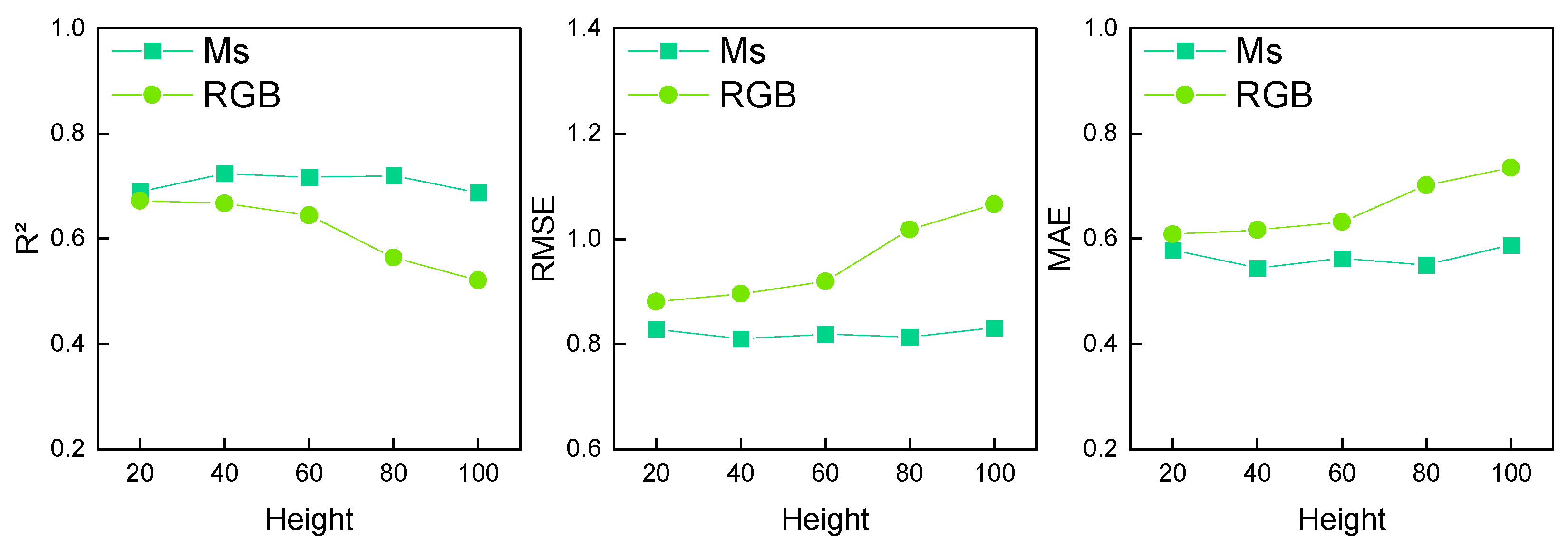
Data Type	20M			40M			60M			80M			100M
	R2	RMSE	MAE	R2	RMSE	MAE	R2	RMSE	MAE	R2	RMSE	MAE	R2	RMSE	MAE
Ms	0.690	0.829	0.579	0.724	0.810	0.545	0.717	0.819	0.563	0.720	0.814	0.551	0.688	0.831	0.588
RGB	0.673	0.881	0.609	0.667	0.896	0.617	0.645	0.919	0.632	0.564	1.018	0.702	0.521	1.066	0.735

and Figure 8, the estimation accuracy of Ms data under spatial resolutions corresponding to different heights shows no significant change pattern, with the highest accuracy at 40 m (2.2 cm), where the R², RMSE, and MAE of the model are 0.724, 0.810, and 0.545, respectively. In contrast, the RGB data show a decrease in the estimation accuracy with the reduction in spatial resolution, and the R² values at 20 m (0.4 cm), 40 m (1.0 cm), 60 m (1.4 cm), 80 m (2.0 cm), and 100 m (2.9 cm) are 0.673, 0.667, 0.645, 0.564, and 0.521, respectively.

Based on the best height and spatial resolution of different data sources, namely, 40 m (2.2 cm) for Ms data and 20 m (0.4 cm) for RGB data, the LAI estimation effects of different data sources under different feature mixes are compared by integrating texture and coverage features. As shown in

Table 10. Accuracy of the LAI model with multi-features mixed from single-data sources.

Data Type	VIs			VIs + M_CC			VIs + M_TFs			VIs + M_TFs + M_CC
Ms	R2	RMSE	MAE	R2	RMSE	MAE	R2	RMSE	MAE	R2	RMSE	MAE
	0.675	0.886	0.659	0.703	0.847	0.527	0.724	0.810	0.545	0.712	0.828	0.573
	CIs			CIs + R_CC			CIs + R_TFs			CIs + R_TFs + R_CC
RGB	R2	RMSE	MAE	R2	RMSE	MAE	R2	RMSE	MAE	R2	RMSE	MAE
	0.607	0.966	0.709	0.671	0.884	0.606	0.673	0.881	0.609	0.668	0.912	0.625

and Figure 9, when M_CC or R_CC is added to the model, the R², RMSE, and MAE of VIs + M_CC accuracy are 0.703, 0.847, and 0.527, and for CIs + R_CC, the accuracy is 0.671, 0.884, and 0.606. This shows that adding CC can improve the model’s estimation accuracy. Moreover, the model estimation results of different data sources are further enhanced after the model adds M_TFs or R_TFs. The R², RMSE, and MAE of VIs + M_TFs accuracy are 0.724, 0.810, and 0.545, and for CIs + R_TFs, the accuracy is 0.673, 0.881, and 0.609. This shows that for Ms data, M_TFs can provide more information than M_CC in estimating LAI, while for RGB data, the enhancement effects of R_TFs and R_CC are comparable. When the model mixes all features, the R², RMSE, and MAE of VIs + M_TFs + M_CC accuracy are 0.712, 0.828, and 0.573, and the + R_TFs + R_CC accuracy of CIs is 0.668, 0.912, and 0.625, values which are not much different from those from the model used to estimate the LAI by adding only TFs. For Ms data, when estimating LAI, the R² of the model with the addition of M_TFs and M_CC improved by 7.3% and 4.1% compared to the VI-only estimation, while for the RGB data, the R² of the model with the addition of R_TFs and R_CC improved by 10.9% and 10.5% over the CI-only estimation in LAI. After adding texture features, the estimation accuracy of different data increased by 9.1% on average, while after adding coverage, it increased by 7.3% on average. This indicates that texture and coverage can make up for the shortcomings of estimating the LAI of rice with only spectral features, with texture features contributing more. However, when the texture and coverage features are integrated, the estimation performance of LAI does not improve, indicating that the model tends to saturate at this point.

Combining RGB and multispectral (Ms) data sources and using RFR as the primary model, nine different mixed modes are selected for analysis to explore the results of LAI estimation under the mutual combination of different data source features: VIs (NDRE, GNDVI, OSAVI, and EVI2), M_TFs (R_NIR-Mea, R_NIR-Hom, R_NIR-Ent, and R_NIR-Sec), M_CC, CIs (EXG, GLA, EXGR, and RGBVI), R_TFs (R-Sec, G-Ent, G-Sec, and B-Sec), and R_CC. The results are shown in

Table 11. Accuracy of the LAI model with multi-features mode mixed from multi-data sources.

Mode	Number of Variables	Feature Mixed	R2	RMSE	MAE
1	8	VIs + CIs	0.725	0.808	0.520
2	9	VIs + CIs + M_CC	0.723	0.817	0.534
3	9	VIs + CIs + R_CC	0.728	0.809	0.517
4	12	VIs + CIs + M_TFs	0.740	0.796	0.489
5	12	VIs + CIs + R_TFs	0.730	0.803	0.510
6	16	VIs + CIs + M_TFs + R_TFs	0.731	0.800	0.509
7	17	VIs + CIs + M_TFs + R_TFs + M_CC	0.722	0.814	0.545
8	17	VIs + CIs + M_TFs + R_TFs + R_CC	0.724	0.814	0.535
9	18	VIs + CIs + M_TFs + R_TFs + M_CC + R_CC	0.729	0.807	0.519

and Figure 10, and it is found that when combining the multi-data source features, the R², RMSE, and MAE of the VIs + CIs of mode 1 are 0.725, 0.808, and 0.520, respectively. Compared with the single-data source, VIs + M_TFs and CIs + R_TFs show higher LAI estimation model accuracy than RGB data, but exhibit little difference with Ms data. Among all the modes, the VIs + CIs + M_TFs of mode 4 had the highest accuracy, with R², RMSE, and MAE vales of up to 0.740, 0.796, and 0.489, and the VIs + CIs + M_TFs + R_TFs + M_CC of mode 7 had the lowest accuracy, with R², RMSE, and MAE values of 0.722, 0.814, and 0.545, respectively. The R² of VIs + CIs + R_TFs + M_CC in Mode 5 was 0.730, which indicated that the M_TFs at the Ms near-infrared band were more sensitive to the vegetation relationship than the RGB feature R_TFs, and could play an important role in the estimation of rice LAI. Compared with mode 1, the accuracy of modes 2, 7, and 8 does not improve, and the model accuracy of mode 9 only slightly improves after all features are mixed, with R², RMSE, and MAE of 0.729, 0.807, and 0.519, respectively. This shows that when combining two data sources, the coverage cannot effectively solve the problem that the model tends to become saturated compared with texture features. This indicates that better estimation can be achieved based on Ms data alone, and when combining the two remote sensing data points to estimate rice LAI, the VI and M_TF features of Ms data and the CI feature of RGB data are the optimal combinations that can play the best role in estimating rice LAI.

4. Discussion

4.1. Comparison of Accuracy between Image Down-Sampling and Data Acquisition by UAV

Image down-sampling can mimic the spatial resolution effect of UAVs at different heights [49,69]. Comparing the results after down-sampling with models at different heights can indirectly ignore the influence of environmental factors and help to comprehensively explore the effect of image spatial resolution on LAI estimation. Based on multispectral (Ms) 20 m (1.1 cm) and RGB 20 m (0.4 cm) data, images from different data sources are down-sampled to the corresponding spatial resolutions of 40 m, 60 m, 80 m, and 100 m. Different height images correspond to different spatial resolutions, and there are differences in different data sources. As shown in Figure 11, RGB true color and Ms false color are used to display local images of rice. Figure 11(II,IV) show that the resampled spatial resolution is prone to salt-and-pepper noise.

Considering the findings in Section 3.3, which indicate that models only with texture features perform the best, VIs + M_TFs and CIs + R_TFs are selected as the comparison objects after down-sampling from different data sources. As shown in Figure 12, there is no significant pattern between the down-sampled multispectral (D_Ms) and the UAV measured Ms in estimating LAI at different heights, and the differences in R² are all within 0.05. However, the performance of the down-sampled RGB (D_RGB) in estimating LAI is similar to that of the RGB measured by the UAV. The estimation accuracy decreases with the increase in height, and the accuracy at 80 m (2.0 cm) and 100 m (2.9 cm) is higher than that of the UAV-measured data. This is mostly due to the fact that both Ms and RGB data are affected by the environment, such as illumination or wind speed, in the actual UAV data acquisition [70,71].

4.2. Effect of Rice Heading on LAI Estimation

As can be seen in the Results section, the results using spectral inversion tend to be saturated after the LAI value exceeds 4, which is largely due to the effect of the panicle [72,73]. To compare the effect of the panicle on rice LAI estimation, we categorized the tillering and jointing stages as the pre-heading stage (Pre-Hs), and the heading and filling stages as the post-heading stage (Pos-Hs). RFR models were established for each stage. As shown in

Table 12. Accuracy of the LAI model in the Pre-Hs and Pos-Hs from single-data sources.

Data Type	VIs			VIs + M_CC			VIs + M_TFs			VIs + M_TFs + M_CC
Ms	R2	RMSE	MAE	R2	RMSE	MAE	R2	RMSE	MAE	R2	RMSE	MAE
Pre-Hs	0.691	0.638	0.464	0.715	0.615	0.446	0.734	0.609	0.424	0.734	0.608	0.427
Pos-Hs	0.420	1.178	0.953	0.456	1.146	0.919	0.449	1.154	0.935	0.443	1.155	0.941
	CIs			CIs + R_CC			CIs + R_TFs			CIs + R_TFs + R_CC
RGB	R2	RMSE	MAE	R2	RMSE	MAE	R2	RMSE	MAE	R2	RMSE	MAE
Pre-Hs	0.618	0.701	0.549	0.677	0.653	0.484	0.689	0.645	0.472	0.683	0.648	0.478
Pos-Hs	0.355	1.239	1.018	0.412	1.183	0.957	0.405	1.191	0.970	0.408	1.189	0.963

, under the mixed features of single-data sources, the LAI estimation accuracy in the Pos-Hs is significantly lower than that in the Pre-Hs. After adding texture features, the accuracy of the model for estimating LAI in the Pre-Hs was improved, and the accuracy of R² for CIs + R_TFs and VIs + M_TFs was 0.689 and 0.734, respectively. The mixed features of VIs + M_TFs + M_CC and VIs + M_CC are the best for Ms data in the Pre-Hs and Pos-Hs. The R², RMSE, and MAE of Pre-Hs are 0.734, 0.608, and 0.427, respectively, and the R², RMSE, and MAE of Pos-Hs are 0.456, 1.146, and 0.919, respectively. The mixed features of CIs + R_TFs and CIs + R_CC are the best for RGB data in the Pre-Hs and Pos-Hs. The R², RMSE, and MAE of the Pre-Hs are 0.689, 0.645, and 0.472, respectively, and the R², RMSE, and MAE of the Pos-Hs are 0.412, 1.183, and 0.957, respectively. It can be seen that the estimation accuracy of LAI after heading is the highest when only the coverage feature is added. Therefore, both Ms and RGB data are affected by the panicle when estimating rice LAI, while the texture and coverage have significant effects on the estimation of rice LAI in the Pre-Hs and Pos-Hs, respectively.

As shown in Figure 13, under the same CC extraction method, the overall result of Ms extraction is larger than that of RGB extraction, which is primarily due to the fact that RGB is more affected by the color of the panicle. For RGB data, color information is highly sensitive, and when green pixels in the Pre-Hs and yellow pixels in the Pos-Hs exist at the same time, a simple classification cannot effectively distinguish different colored canopies from the background. Therefore, by combining the change rule of the RGB combination value from light yellow RGB (64,64,0) to medium yellow RGB (128,128,0) to dark yellow RGB (255,255,0), it can be seen that simultaneously and isometrically amplifying the values of the R and G channels while reducing the values of the B channel can effectively identify the yellow canopy pixels. Based on this idea, EXR is added to EXG; that is, the RGB canopy panicle pixels are extracted by EXG + EXR, and the R_CC incorporated into the panicle is recorded as R_CC’. As shown in Figure 13g, the ability to estimate rice LAI based on CIs features was compared with the R_CC’ after adding panicle pixels. The accuracy R² of CIs + R_CC’ and CIs + R_TFs + R_CC’ of the model in the Pos-Hs is 0.438 and 0.440, respectively, representing improvements of 6.3% and 7.8% compared to the previous values. This indicated that compared with the CC with only leaves, the CC with panicle pixels could improve the RGB estimation of rice LAI, which was mostly due to the fact that the panicle pixels provided more canopy structure and density distribution after rice in the Pos-Hs, although the panicle caused the leaves to block the canopy, which simply compensated for the extra information needed for LAI inversion.

4.3. Analysis of the Application Potential of the Research Results

With the recent reduction in UAV costs, low-altitude remote sensing has become more widely used in agriculture [74]. Particularly in estimating LAI by UAV, Sun et al. [71] extracted the color index of the RGB image and estimated the R² of rice LAI by MLR as 0.5–0.57, and their conclusion showed that RGB was greatly influenced by illumination and image background changes. This corresponds to the conclusion obtained in this paper, that is, the accuracy of estimating rice LAI with RGB data decreases with the increase in height, which shows that RGB is more affected by light attenuation and atmospheric scattering at different heights than multispectral (Ms) scattering. Sun et al. [71] did not further discuss the texture features of RGB, but in this paper, the estimation accuracy of the LAI was improved by the RGB texture and coverage features, which was consistent with the results of Liu et al. [75] in estimating biomass. Consistent with the research of Zou et al. [76], when considering the combination of spectral and texture features of multi-spectra, the R² of winter wheat LAI estimated by RF at a 95.5 m flying height was 0.68, which is similar to the R² estimated by RF at a height of 100 m in this study. This indicates that the combination of texture and spectral features can improve the estimation accuracy of crop LAI, but it has not been discussed further different flying heights and spatial resolutions. In addition, Zou et al. [76] improved XGBoost and RF accuracy by adding plant height, outperforming CNN and LSTM deep learning methods, though Zu et al. [77] indicated that CNN slightly surpassed RF in LAI estimation. This suggests that the applicability of deep learning models for LAI estimation requires further exploration. In this study, the estimation accuracy of LAI has been improved to a certain extent after adding coverage features. It can be seen that crop monitoring that integrates crop phenotypic parameters will be one of the key aspects of future research, whether it refers to plant height or coverage features. Furthermore, the research results of Du et al. [78] show that the ensemble learning method based on the stacking of multiple machine learning models is superior to the single machine learning model in estimating the LAI of rapeseed, which is consistent with the conclusion of Liu et al. [79]. While this study does not analyze ensemble learning, it offers insights for selecting base models for such methods. Yu et al. [80] estimated the LAI of rice using a multi-modal fusion method KF-DGDV, and the R² was 0.76 at the tillering to booting stage and 0.66 at the filling stage. This difference corresponds to the conclusion of the discussion in Section 4.2 of this paper. Therefore, we come to the conclusion that the main reason for this phenomenon is that the leaves of rice essentially stop growing at the late growth stage, while the panicle absorbs most nutrients [72], which leads to the saturation of the LAI. Although the complementarity of multi-source UAV data can make up for the deficiency of remote sensing in crop growth monitoring [81], and VIs + CIs + M_TFs combined with multi-source data are the most effective in this study, this does not explain the applicability and stability of this combination in different crops and different fertilization management plots. Therefore, the combined use of multi-source UAV data and their inherent complementary effects need to be further studied in the future.

UAV has been widely used because of its advantages of high efficiency and low cost, but the application of large-scale plots is an irreparable shortcoming of UAV, which can be well satisfied by satellite remote sensing, but at the same time, satellite remote sensing has the problems of low revisit period and resolution. The existing research shows that there is great potential for UAV-satellite to accurately estimate large area vegetation biomass by matching UAV-satellite remote sensing data [82], but there is little research on the deep combination of multi-band information of satellite remote sensing. Therefore, considering crop phenotypic information combined with multi-source remote sensing data will be the focus of our future research, and this is also crucial to realize crop monitoring and decision management.

5. Conclusions

This study utilized multi-source remote sensing data from UAVs at different flying heights to estimate rice LAI, aiming to explore the effect of different spatial resolutions on RGB and multispectral (Ms) data in estimating rice LAI, and the optimal model height under different mixtures of features. The results indicate that for flying heights between 20–100 m, both RGB and Ms data are best represented by the RFR model with multi-feature inputs. The effect of different spatial resolutions on rice LAI estimation using Ms data was minimal, with the best results at 40 m (2.2 cm). For RGB data, accuracy decreased as spatial resolution decreased. Ms data consistently outperformed RGB data across different spatial resolutions, and the result of RGB is best at 20 m (0.4 cm). Adding coverage or texture features improved LAI estimation accuracy for both Ms and RGB data. Combining different data sources revealed that the optimal results were achieved by mixing VIs and M_TFs features from Ms data with CIs features from RGB data. The study also controlled for environmental factors through resampling, showing that resampling and different flight heights had similar patterns in LAI estimation, with the smallest difference in Ms data and an increase in RGB data differences after 60 m (1.4 cm). This shows that for RGB data, flying heights of 80–100 m are more susceptible to environmental influence. The presence of heading affected LAI estimation, with poor RGB canopy coverage extraction caused by panicle interference. However, we improved the accuracy of LAI estimation of RGB data by integrating spike information with EXG + EXR. These findings provide a valuable reference for accurate rice LAI estimation and for selecting models and determining optimal spatial resolutions.

References

- Van Nguyen, N.; Ferrero, A. Meeting the challenges of global rice production. Paddy Water Environ. 2006, 4, 1–9. [Google Scholar] [CrossRef]
- Muthayya, S.; Sugimoto, J.D.; Montgomery, S.; Maberly, G.F. An overview of global rice production, supply, trade, and consumption. Ann. N. Y. Acad. Sci. 2014, 1324, 7–14. [Google Scholar] [CrossRef]
- Tang, L.; Risalat, H.; Cao, R.; Hu, Q.; Pan, X.; Hu, Y.; Zhang, G. Food Security in China: A Brief View of Rice Production in Recent 20 Years. Foods 2022, 11, 3324. [Google Scholar] [CrossRef] [PubMed]
- Bandumula, N. Rice Production in Asia: Key to Global Food Security. Proc. Natl. Acad. Sci. India Sect. B Biol. Sci. 2017, 88, 1323–1328. [Google Scholar] [CrossRef]
- Qiu, Z.; Ma, F.; Li, Z.; Xu, X.; Ge, H.; Du, C. Estimation of nitrogen nutrition index in rice from UAV RGB images coupled with machine learning algorithms. Comput. Electron. Agric. 2021, 189, 106421. [Google Scholar] [CrossRef]
- Yan, G.; Hu, R.; Luo, J.; Weiss, M.; Jiang, H.; Mu, X.; Xie, D.; Zhang, W. Review of indirect optical measurements of leaf area index: Recent advances, challenges, and perspectives. Agric. For. Meteorol. 2019, 265, 390–411. [Google Scholar] [CrossRef]
- Jonckheere, I.; Fleck, S.; Nackaerts, K.; Muys, B.; Coppin, P.; Weiss, M.; Baret, F. Review of methods for in situ leaf area index determination: Part I. Theories, sensors and hemispherical photography. Agric. For. Meteorol. 2004, 121, 19–35. [Google Scholar] [CrossRef]
- Fang, H.; Baret, F.; Plummer, S.; Schaepman-Strub, G. An Overview of Global Leaf Area Index (LAI): Methods, Products, Validation, and Applications. Rev. Geophys. 2019, 57, 739–799. [Google Scholar] [CrossRef]
- Rosati, A. Estimating Canopy Light Interception and Absorption Using Leaf Mass Per Unit Leaf Area in Solanum melongena. Ann. Bot. 2001, 88, 101–109. [Google Scholar] [CrossRef]
- Weiss, M.; Baret, F.; Smith, G.J.; Jonckheere, I.; Coppin, P. Review of methods for in situ leaf area index (LAI) determination: Part II. Estimation of LAI, errors and sampling. Agric. For. Meteorol. 2004, 121, 37–53. [Google Scholar] [CrossRef]
- Fang, H.; Li, W.; Wei, S.; Jiang, C. Seasonal variation of leaf area index (LAI) over paddy rice fields in NE China: Intercomparison of destructive sampling, LAI-2200, digital hemispherical photography (DHP), and AccuPAR methods. Agric. For. Meteorol. 2014, 198–199, 126–141. [Google Scholar] [CrossRef]
- Yang, R.; Liu, L.; Liu, Q.; Li, X.; Yin, L.; Hao, X.; Ma, Y.; Song, Q. Validation of leaf area index measurement system based on wireless sensor network. Sci. Rep. 2022, 12, 4668. [Google Scholar] [CrossRef] [PubMed]
- Confalonieri, R.; Foi, M.; Casa, R.; Aquaro, S.; Tona, E.; Peterle, M.; Boldini, A.; De Carli, G.; Ferrari, A.; Finotto, G.; et al. Development of an app for estimating leaf area index using a smartphone. Trueness and precision determination and comparison with other indirect methods. Comput. Electron. Agric. 2013, 96, 67–74. [Google Scholar] [CrossRef]
- Johnson, L.; Roczen, D.; Youkhana, S.; Nemani, R.; Bosch, D. Mapping vineyard leaf area with multispectral satellite imagery. Comput. Electron. Agric. 2003, 38, 33–44. [Google Scholar] [CrossRef]
- Qiao, L.; Gao, D.; Zhao, R.; Tang, W.; An, L.; Li, M.; Sun, H. Improving estimation of LAI dynamic by fusion of morphological and vegetation indices based on UAV imagery. Comput. Electron. Agric. 2022, 192, 106603. [Google Scholar] [CrossRef]
- Zheng, G.; Moskal, L.M. Retrieving Leaf Area Index (LAI) Using Remote Sensing: Theories, Methods and Sensors. Sensors 2009, 9, 2719–2745. [Google Scholar] [CrossRef]
- Jacquemoud, S.; Verhoef, W.; Baret, F.; Bacour, C.; Zarco-Tejada, P.J.; Asner, G.P.; François, C.; Ustin, S.L. PROSPECT+SAIL models: A review of use for vegetation characterization. Remote Sens. Environ. 2009, 113, S56–S66. [Google Scholar] [CrossRef]
- Wei, C.; Huang, J.; Mansaray, L.; Li, Z.; Liu, W.; Han, J. Estimation and Mapping of Winter Oilseed Rape LAI from High Spatial Resolution Satellite Data Based on a Hybrid Method. Remote Sens. 2017, 9, 488. [Google Scholar] [CrossRef]
- Wang, Y.; Fang, H. Estimation of LAI with the LiDAR Technology: A Review. Remote Sens. 2020, 12, 3457. [Google Scholar] [CrossRef]
- Wu, M.; Wu, C.; Huang, W.; Niu, Z.; Wang, C. High-resolution Leaf Area Index estimation from synthetic Landsat data generated by a spatial and temporal data fusion model. Comput. Electron. Agric. 2015, 115, 1–11. [Google Scholar] [CrossRef]
- Tian, J.; Wang, L.; Li, X.; Gong, H.; Shi, C.; Zhong, R.; Liu, X. Comparison of UAV and WorldView-2 imagery for mapping leaf area index of mangrove forest. Int. J. Appl. Earth Obs. Geoinf. 2017, 61, 22–31. [Google Scholar] [CrossRef]
- Tsouros, D.C.; Bibi, S.; Sarigiannidis, P.G. A Review on UAV-Based Applications for Precision Agriculture. Information 2019, 10, 349. [Google Scholar] [CrossRef]
- Olson, D.; Anderson, J. Review on unmanned aerial vehicles, remote sensors, imagery processing, and their applications in agriculture. Agron. J. 2021, 113, 971–992. [Google Scholar] [CrossRef]
- Xie, C.; Yang, C. A review on plant high-throughput phenotyping traits using UAV-based sensors. Comput. Electron. Agric. 2020, 178, 105731. [Google Scholar] [CrossRef]
- Shi, Y.; Gao, Y.; Wang, Y.; Luo, D.; Chen, S.; Ding, Z.; Fan, K. Using Unmanned Aerial Vehicle-Based Multispectral Image Data to Monitor the Growth of Intercropping Crops in Tea Plantation. Front. Plant Sci. 2022, 13, 820585. [Google Scholar] [CrossRef]
- Lin, Y. LiDAR: An important tool for next-generation phenotyping technology of high potential for plant phenomics? Comput. Electron. Agric. 2015, 119, 61–73. [Google Scholar] [CrossRef]
- Zhang, F.; Hassanzadeh, A.; Kikkert, J.; Pethybridge, S.J.; van Aardt, J. Evaluation of Leaf Area Index (LAI) of Broadacre Crops Using UAS-Based LiDAR Point Clouds and Multispectral Imagery. IEEE J. Sel. Top. Appl. Earth Obs. Remote Sens. 2022, 15, 4027–4044. [Google Scholar] [CrossRef]
- Luo, S.; Chen, J.M.; Wang, C.; Gonsamo, A.; Xi, X.; Lin, Y.; Qian, M.; Peng, D.; Nie, S.; Qin, H. Comparative Performances of Airborne LiDAR Height and Intensity Data for Leaf Area Index Estimation. IEEE J. Sel. Top. Appl. Earth Obs. Remote Sens. 2018, 11, 300–310. [Google Scholar] [CrossRef]
- Li, S.; Yuan, F.; Ata-Ui-Karim, S.T.; Zheng, H.; Cheng, T.; Liu, X.; Tian, Y.; Zhu, Y.; Cao, W.; Cao, Q. Combining Color Indices and Textures of UAV-Based Digital Imagery for Rice LAI Estimation. Remote Sens. 2019, 11, 1763. [Google Scholar] [CrossRef]
- Zhang, Y.; Ta, N.; Guo, S.; Chen, Q.; Zhao, L.; Li, F.; Chang, Q. Combining Spectral and Textural Information from UAV RGB Images for Leaf Area Index Monitoring in Kiwifruit Orchard. Remote Sens. 2022, 14, 1063. [Google Scholar] [CrossRef]
- Zhang, X.; Zhang, K.; Sun, Y.; Zhao, Y.; Zhuang, H.; Ban, W.; Chen, Y.; Fu, E.; Chen, S.; Liu, J.; et al. Combining Spectral and Texture Features of UAS-Based Multispectral Images for Maize Leaf Area Index Estimation. Remote Sens. 2022, 14, 331. [Google Scholar] [CrossRef]
- Yuan, W.; Meng, Y.; Li, Y.; Ji, Z.; Kong, Q.; Gao, R.; Su, Z. Research on rice leaf area index estimation based on fusion of texture and spectral information. Comput. Electron. Agric. 2023, 211, 108016. [Google Scholar] [CrossRef]
- Zhang, Y.; Yang, Y.; Zhang, Q.; Duan, R.; Liu, J.; Qin, Y.; Wang, X. Toward Multi-Stage Phenotyping of Soybean with Multimodal UAV Sensor Data: A Comparison of Machine Learning Approaches for Leaf Area Index Estimation. Remote Sens. 2022, 15, 7. [Google Scholar] [CrossRef]
- Carlson, T.N.; Ripley, D.A. On the relation between NDVI, fractional vegetation cover, and leaf area index. Remote Sens. Environ. 1997, 62, 241–252. [Google Scholar] [CrossRef]
- Xiao, Z.; Wang, T.; Liang, S.; Sun, R. Estimating the Fractional Vegetation Cover from GLASS Leaf Area Index Product. Remote Sens. 2016, 8, 337. [Google Scholar] [CrossRef]
- Zhang, D.; Liu, J.; Ni, W.; Sun, G.; Zhang, Z.; Liu, Q.; Wang, Q. Estimation of forest leaf area index using height and canopy cover information extracted from unmanned aerial vehicle stereo imagery. IEEE J. Sel. Top. Appl. Earth Obs. Remote Sens. 2019, 12, 471–481. [Google Scholar] [CrossRef]
- Wang, F.-m.; Huang, J.-f.; Lou, Z.-h. A comparison of three methods for estimating leaf area index of paddy rice from optimal hyperspectral bands. Precis. Agric. 2010, 12, 439–447. [Google Scholar] [CrossRef]
- Siegmann, B.; Jarmer, T. Comparison of different regression models and validation techniques for the assessment of wheat leaf area index from hyperspectral data. Int. J. Remote Sens. 2015, 36, 4519–4534. [Google Scholar] [CrossRef]
- Colombo, R. Retrieval of leaf area index in different vegetation types using high resolution satellite data. Remote Sens. Environ. 2003, 86, 120–131. [Google Scholar] [CrossRef]
- Nguyen, H.T.; Lee, B.-W. Assessment of rice leaf growth and nitrogen status by hyperspectral canopy reflectance and partial least square regression. Eur. J. Agron. 2006, 24, 349–356. [Google Scholar] [CrossRef]
- Li, X.; Zhang, Y.; Bao, Y.; Luo, J.; Jin, X.; Xu, X.; Song, X.; Yang, G. Exploring the Best Hyperspectral Features for LAI Estimation Using Partial Least Squares Regression. Remote Sens. 2014, 6, 6221–6241. [Google Scholar] [CrossRef]
- Durbha, S.S.; King, R.L.; Younan, N.H. Support vector machines regression for retrieval of leaf area index from multiangle imaging spectroradiometer. Remote Sens. Environ. 2007, 107, 348–361. [Google Scholar] [CrossRef]
- Liang, L.; Di, L.; Huang, T.; Wang, J.; Lin, L.; Wang, L.; Yang, M. Estimation of Leaf Nitrogen Content in Wheat Using New Hyperspectral Indices and a Random Forest Regression Algorithm. Remote Sens. 2018, 10, 1940. [Google Scholar] [CrossRef]
- Chen, Z.; Jia, K.; Xiao, C.; Wei, D.; Zhao, X.; Lan, J.; Wei, X.; Yao, Y.; Wang, B.; Sun, Y.; et al. Leaf Area Index Estimation Algorithm for GF-5 Hyperspectral Data Based on Different Feature Selection and Machine Learning Methods. Remote Sens. 2020, 12, 2110. [Google Scholar] [CrossRef]
- Zhang, J.; Wang, C.; Yang, C.; Xie, T.; Jiang, Z.; Hu, T.; Luo, Z.; Zhou, G.; Xie, J. Assessing the effect of real spatial resolution of in situ UAV multispectral images on seedling rapeseed growth monitoring. Remote Sens. 2020, 12, 1207. [Google Scholar] [CrossRef]
- Petras, V.; Petrasova, A.; McCarter, J.B.; Mitasova, H.; Meentemeyer, R.K. Point Density Variations in Airborne Lidar Point Clouds. Sensors 2023, 23, 1593. [Google Scholar] [CrossRef]
- Kamal, M.; Phinn, S.; Johansen, K. Assessment of multi-resolution image data for mangrove leaf area index mapping. Remote Sens. Environ. 2016, 176, 242–254. [Google Scholar] [CrossRef]
- Li, W.; Wang, J.; Zhang, Y.; Yin, Q.; Wang, W.; Zhou, G.; Huo, Z. Combining Texture, Color, and Vegetation Index from Unmanned Aerial Vehicle Multispectral Images to Estimate Winter Wheat Leaf Area Index during the Vegetative Growth Stage. Remote Sens. 2023, 15, 5715. [Google Scholar] [CrossRef]
- Yue, J.; Yang, G.; Tian, Q.; Feng, H.; Xu, K.; Zhou, C. Estimate of winter-wheat above-ground biomass based on UAV ultrahigh-ground-resolution image textures and vegetation indices. ISPRS J. Photogramm. Remote Sens. 2019, 150, 226–244. [Google Scholar] [CrossRef]
- Guo, A.; Ye, H.; Huang, W.; Qian, B.; Wang, J.; Lan, Y.; Wang, S. Inversion of maize leaf area index from UAV hyperspectral and multispectral imagery. Comput. Electron. Agric. 2023, 212, 108020. [Google Scholar] [CrossRef]
- Lyu, X.; Li, X.; Gong, J.; Li, S.; Dou, H.; Dang, D.; Xuan, X.; Wang, H. Remote-sensing inversion method for aboveground biomass of typical steppe in Inner Mongolia, China. Ecol. Indic. 2021, 120, 106883. [Google Scholar] [CrossRef]
- Kira, O.; Nguy-Robertson, A.L.; Arkebauer, T.J.; Linker, R.; Gitelson, A.A. Toward Generic Models for Green LAI Estimation in Maize and Soybean: Satellite Observations. Remote Sens. 2017, 9, 318. [Google Scholar] [CrossRef]
- Liu, Y.; Fan, Y.; Feng, H.; Chen, R.; Bian, M.; Ma, Y.; Yue, J.; Yang, G. Estimating potato above-ground biomass based on vegetation indices and texture features constructed from sensitive bands of UAV hyperspectral imagery. Comput. Electron. Agric. 2024, 220, 108918. [Google Scholar] [CrossRef]
- Sekrecka, A.; Wierzbicki, D.; Kedzierski, M. Influence of the Sun Position and Platform Orientation on the Quality of Imagery Obtained from Unmanned Aerial Vehicles. Remote Sens. 2020, 12, 1040. [Google Scholar] [CrossRef]
- Kennedy, S.; Burbach, M. Great Plains Ranchers Managing for Vegetation Heterogeneity: A Multiple Case Study. Great Plains Res. 2020, 30, 137–148. [Google Scholar] [CrossRef]
- Gitelson, A.A.; Kaufman, Y.J.; Stark, R.; Rundquist, D. Novel algorithms for remote estimation of vegetation fraction. Remote Sens. Environ. 2002, 80, 76–87. [Google Scholar] [CrossRef]
- Gitelson, A.A.; Kaufman, Y.J.; Merzlyak, M.N. Use of a green channel in remote sensing of global vegetation from EOS-MODIS. Remote Sens. Environ. 1996, 58, 289–298. [Google Scholar] [CrossRef]
- Fitzgerald, G.J.; Rodriguez, D.; Christensen, L.K.; Belford, R.; Sadras, V.O.; Clarke, T.R. Spectral and thermal sensing for nitrogen and water status in rainfed and irrigated wheat environments. Precis. Agric. 2006, 7, 233–248. [Google Scholar] [CrossRef]
- Jiang, Z.; Huete, A.; Didan, K.; Miura, T. Development of a two-band enhanced vegetation index without a blue band. Remote Sens. Environ. 2008, 112, 3833–3845. [Google Scholar] [CrossRef]
- Rondeaux, G.; Steven, M.; Baret, F. Optimization of soil-adjusted vegetation indices. Remote Sens. Environ. 1996, 55, 95–107. [Google Scholar] [CrossRef]
- Panigada, C.; Rossini, M.; Busetto, L.; Meroni, M.; Fava, F.; Colombo, R. Chlorophyll concentration mapping with MIVIS data to assess crown discoloration in the Ticino Park oak forest. Int. J. Remote Sens. 2010, 31, 3307–3332. [Google Scholar] [CrossRef]
- Gitelson, A.A.; Viña, A.; Ciganda, V.; Rundquist, D.C.; Arkebauer, T.J. Remote estimation of canopy chlorophyll content in crops. Geophys. Res. Lett. 2005, 32, L08403. [Google Scholar] [CrossRef]
- Meyer, G.E.; Hindman, T.W.; Laksmi, K. Machine vision detection parameters for plant species identification. In Proceedings of the Precision Agriculture and Biological Quality, Boston, MA, USA, 3–4 November 1999; pp. 327–335. [Google Scholar]
- Meyer, G.E.; Neto, J.C. Verification of color vegetation indices for automated crop imaging applications. Comput. Electron. Agric. 2008, 63, 282–293. [Google Scholar] [CrossRef]
- Mao, W.; Wang, Y.; Wang, Y. Real-time detection of between-row weeds using machine vision. In Proceedings of the 2003 ASAE Annual Meeting, Las Vegas, NV, USA, 27–30 July 2003; p. 1. [Google Scholar]
- Louhaichi, M.; Borman, M.M.; Johnson, D.E. Spatially Located Platform and Aerial Photography for Documentation of Grazing Impacts on Wheat. Geocarto Int. 2001, 16, 65–70. [Google Scholar] [CrossRef]
- Tucker, C.J. Red and photographic infrared linear combinations for monitoring vegetation. Remote Sens. Environ. 1979, 8, 127–150. [Google Scholar] [CrossRef]
- Bendig, J.; Yu, K.; Aasen, H.; Bolten, A.; Bennertz, S.; Broscheit, J.; Gnyp, M.L.; Bareth, G. Combining UAV-based plant height from crop surface models, visible, and near infrared vegetation indices for biomass monitoring in barley. Int. J. Appl. Earth Obs. Geoinf. 2015, 39, 79–87. [Google Scholar] [CrossRef]
- Seifert, E.; Seifert, S.; Vogt, H.; Drew, D.; van Aardt, J.; Kunneke, A.; Seifert, T. Influence of Drone Altitude, Image Overlap, and Optical Sensor Resolution on Multi-View Reconstruction of Forest Images. Remote Sens. 2019, 11, 1252. [Google Scholar] [CrossRef]
- Feng, L.; Wu, W.; Wang, J.; Zhang, C.; Zhao, Y.; Zhu, S.; He, Y. Wind Field Distribution of Multi-rotor UAV and Its Influence on Spectral Information Acquisition of Rice Canopies. Remote Sens. 2019, 11, 602. [Google Scholar] [CrossRef]
- Sun, B.; Li, Y.; Huang, J.; Cao, Z.; Peng, X. Impacts of Variable Illumination and Image Background on Rice LAI Estimation Based on UAV RGB-Derived Color Indices. Appl. Sci. 2024, 14, 3214. [Google Scholar] [CrossRef]
- He, J.; Zhang, N.; Su, X.; Lu, J.; Yao, X.; Cheng, T.; Zhu, Y.; Cao, W.; Tian, Y. Estimating Leaf Area Index with a New Vegetation Index Considering the Influence of Rice Panicles. Remote Sens. 2019, 11, 1809. [Google Scholar] [CrossRef]
- Makino, Y.; Hirooka, Y.; Homma, K.; Kondo, R.; Liu, T.-S.; Tang, L.; Nakazaki, T.; Xu, Z.-J.; Shiraiwa, T. Effect of flag leaf length of erect panicle rice on the canopy structure and biomass production after heading. Plant Prod. Sci. 2022, 25, 1–10. [Google Scholar] [CrossRef]
- Zhang, H.; Wang, L.; Tian, T.; Yin, J. A Review of Unmanned Aerial Vehicle Low-Altitude Remote Sensing (UAV-LARS) Use in Agricultural Monitoring in China. Remote Sens. 2021, 13, 1221. [Google Scholar] [CrossRef]
- Liu, Y.; Feng, H.; Yue, J.; Fan, Y.; Bian, M.; Ma, Y.; Jin, X.; Song, X.; Yang, G. Estimating potato above-ground biomass by using integrated unmanned aerial system-based optical, structural, and textural canopy measurements. Comput. Electron. Agric. 2023, 213, 108229. [Google Scholar] [CrossRef]
- Zou, M.; Liu, Y.; Fu, M.; Li, C.; Zhou, Z.; Meng, H.; Xing, E.; Ren, Y. Combining spectral and texture feature of UAV image with plant height to improve LAI estimation of winter wheat at jointing stage. Front. Plant Sci. 2023, 14, 1272049. [Google Scholar] [CrossRef] [PubMed]
- Zu, J.; Yang, H.; Wang, J.; Cai, W.; Yang, Y. Inversion of winter wheat leaf area index from UAV multispectral images: Classical vs. deep learning approaches. Front. Plant Sci. 2024, 15, 1367828. [Google Scholar] [CrossRef] [PubMed]
- Du, R.; Lu, J.; Xiang, Y.; Zhang, F.; Chen, J.; Tang, Z.; Shi, H.; Wang, X.; Li, W. Estimation of winter canola growth parameter from UAV multi-angular spectral-texture information using stacking-based ensemble learning model. Comput. Electron. Agric. 2024, 222, 109074. [Google Scholar] [CrossRef]
- Liu, Z.; Ji, Y.; Ya, X.; Liu, R.; Liu, Z.; Zong, X.; Yang, T. Ensemble Learning for Pea Yield Estimation Using Unmanned Aerial Vehicles, Red Green Blue, and Multispectral Imagery. Drones 2024, 8, 227. [Google Scholar] [CrossRef]
- Yu, M.; He, J.; Li, W.; Zheng, H.; Wang, X.; Yao, X.; Cheng, T.; Zhang, X.; Zhu, Y.; Cao, W.; et al. Estimation of Rice Leaf Area Index Utilizing a Kalman Filter Fusion Methodology Based on Multi-Spectral Data Obtained from Unmanned Aerial Vehicles (UAVs). Remote Sens. 2024, 16, 2073. [Google Scholar] [CrossRef]
- Liu, Y.; Feng, H.; Yue, J.; Jin, X.; Fan, Y.; Chen, R.; Bian, M.; Ma, Y.; Song, X.; Yang, G. Improved potato AGB estimates based on UAV RGB and hyperspectral images. Comput. Electron. Agric. 2023, 214, 108260. [Google Scholar] [CrossRef]
- Niu, X.; Chen, B.; Sun, W.; Feng, T.; Yang, X.; Liu, Y.; Liu, W.; Fu, B. Estimation of Coastal Wetland Vegetation Aboveground Biomass by Integrating UAV and Satellite Remote Sensing Data. Remote Sens. 2024, 16, 2760. [Google Scholar] [CrossRef]