Article

How Can Seasonality Influence the Performance of Recent Microwave Satellite Soil Moisture Products?

1
School of Engineering, University of Basilicata, 85100 Potenza, Italy
2
Institute of Methodologies for Environmental Analysis IMAA, Italian National Research Council CNR, 85050 Tito Scalo, Italy
3
Department of Civil, Architectural and Environmental Engineering, University of Naples Federico II, 80138 Napoli, Italy
4
Department of Bioresource Engineering, McGill University, Macdonald-Stewart Building, Sainte-Anne-de-Bellevue, QC MS1-026, Canada
*
Author to whom correspondence should be addressed.
Remote Sens. 2024, 16(16), 3044; https://doi.org/10.3390/rs16163044
Submission received: 27 June 2024 / Revised: 6 August 2024 / Accepted: 15 August 2024 / Published: 19 August 2024
(This article belongs to the Special Issue Remote Sensing of Climate-Related Hazards)

Abstract

:
In addition to technical issues related to the instruments used, differences between soil moisture (SM) measured using ground-based methods and microwave remote sensing (RS) can be related to the main features of the study areas, which are intricately connected to hydraulic–hydrological conditions and soil properties. When long-term analysis is performed, these discrepancies are mitigated by the contribution of SM seasonality and are only evident when high-frequency variations (i.e., signal anomalies) are investigated. This study sought to examine the responsiveness of SM to seasonal variations in terrestrial ecoregions located in areas covered by the in situ Romanian Soil Moisture Network (RSMN). To achieve this aim, several remote sensing-derived retrievals were considered: (i) NASA’s Soil Moisture Active and Passive (SMAP) L4 V5 model assimilated product data; (ii) the European Space Agency’s Soil Moisture and Ocean Salinity INRA–CESBIO (SMOS-IC) V2.0 data; (iii) time-series data extracted from the H115 and H116 SM products, which are derived from the analysis of Advanced Scatterometer (ASCAT) data acquired via MetOp satellites; (iv) Copernicus Global Land Service SSM 1 km data; and (v) the “combined” European Space Agency’s Climate Change Initiative for Soil Moisture (ESA CCI SM) product v06.1. An initial assessment of the performance of these products was conducted by checking the anomaly of long-term fluctuations, quantified using the Absolute Variation of Local Change of Environment (ALICE) index, within a time frame spanning 2015 to 2020. These correlations were then compared with those based on raw data and anomalies computed using a moving window of 35 days. Prominent correlations were observed with the SMAP L4 dataset and across all ecoregions, and the Balkan mixed forests (646) exhibited strong concordance regardless of the satellite source (with a correlation coefficient RALICE > 0.5). In contrast, neither the Central European mixed forests (No. 654) nor the Pontic steppe (No. 735) were adequately characterized by any satellite dataset (RALICE < 0.5). Subsequently, the phenological seasonality and dynamic behavior of SM were computed to investigate the effects of the wetting and drying processes. Notably, the Central European mixed forests (654) underwent an extended dry phase (with an extremely low p-value of 2.20 × 10⁻¹⁶) during both the growth and dormancy phases. This finding explains why the RSMN showcases divergent behavior and underscores why no satellite dataset can effectively capture the complexities of the ecoregions covered by this in situ SM network.

Graphical Abstract

1. Introduction

Soil moisture (SM) plays a key role in the carbon and water cycles, affecting plant growth and decomposition processes [1,2]. Over the last 15 years, the role of SM as a central factor in the soil–vegetation–climate system has been widely investigated, mostly using microwave satellite instruments. Data acquired in this spectral range are preferred because they can be collected continuously throughout the day and in all weather conditions, being independent of the presence of a natural source of energy (i.e., the sun), and are little affected by interactions with atmospheric constituents [3]. Such data have been used by different space agencies [e.g., the National Aeronautics and Space Administration (NASA) and European Space Agency (ESA)] to produce various continental and/or global-scale SM datasets [3,4].
The accuracy assessment of these large-scale datasets usually involves their comparisons with in situ SM data acquired at diverse monitoring stations, often aggregated within specific networks that can cover different spatial scales (i.e., local, regional, continental). The long-term accuracy of these datasets is positively affected by SM seasonality. When microwave data are used to provide soil moisture information, the latter refers to a superficial soil layer of a few centimeters [5]. Considering that this layer is typically affected by meteorological forcing, when a long-term analysis is conducted, soil moisture seasonality tends to be similar to that of the hydrometeorological pattern in a specific area and, therefore, positively affects the comparison between in situ and satellite SM data. Hence, to obtain a better understanding of the capability of satellite data products to retrieve accurate SM information, it is essential to remove seasonality from the investigated time series [6,7,8,9].
In long-term analysis, the SM signal is a combination of two main contributions: (i) natural seasonal variations from rainfall and evaporation, and (ii) anomalies due to human activities and/or extreme weather. In signal decomposition, SM anomalies are residuals classified as short- or long-term variations based on their relationship with seasonality and how they are computed.
  • Short-term anomalies, i.e., high-frequency, sub-seasonal changes indicating short-term drying and wetting events.
  • Long-term anomalies that include both short-term events and deviations from the long-term mean seasonal cycle, known as SM climatology [10].
SM climatology is vital for spatial modeling and understanding long-term temporal changes [11]. Research into its temporal and seasonal variations in remote sensing remains an open challenge [12,13,14,15].
In addition, when a large area is considered for the comparison between ground and remotely acquired SM data, it is worth noting that climate variability is affected by plant growth and transpiration within the soil–plant system. Therefore, it is important to examine plant phenology and the development of plant organs, focusing on bud break, the growth phases, and dormancy [16]. To understand its link with the climate system, vegetation phenology has frequently been studied using remote sensing (RS) and spectral indices [17,18]. However, few studies have connected SM with phenology owing to the challenges involved in obtaining accurate SM data in dense vegetation.
In a previous paper [19], the authors compared at the ecoregion scale across Europe the performance of the International Soil Moisture Network (ISMN) and ERA5-Land modeled data to that of some SM products: (i) the satellite-derived modeled Soil Moisture Active Passive Level 4 (SMAP L4), (ii) the satellite products Soil Moisture Ocean Salinity INRA–CESBIO (SMOS-IC), (iii) the Advanced SCATterometer (ASCAT), (iv) the Copernicus Global Land Service Surface Soil Moisture (CGLS SSM) at 1 km, and (v) the “combined” satellite retrieval ESA Climate Change Initiative (ESA CCI). That work provided useful insights into how the performance of selected SM satellite products can be affected by both the main features of the products and the selected study area. The results highlighted areas/ecoregions where all satellite products were highly reliable as well as ecoregions where measurements were unreliable regardless of the satellite used. This led us to speculate that there were problems at the ground-based stations. However, distinctly different satellite performances were observed in ecoregions that share the same in situ networks.
Therefore, in the present study, we would like to focus more closely on the contribution of seasonality, in terms of long-term variation and the phenological cycle, to satellite and in situ SM miscorrelation. To better assess the performance of the different SM products, we moved from the analysis of short-term SM variations to more long-term variations (i.e., signal anomalies).
In addition, we investigated the impact of the phenological cycle (i.e., the phases of vegetation growth and dormancy) on SM dynamics. SM levels are closely related to seasonality, and SM dynamics depend on the mutual link between vegetation and water availability, which changes seasonally. To consider both of these factors, we investigated the SM distribution function in each ecoregion, considering the vegetation growth and dormancy phases separately.
The SM frequency analysis is frequently employed to characterize SM dynamics [20,21], and many studies have focused on retrieving the Root Zone SM (RZSM) from surface measurements. For instance, Manfreda et al. [22] analyzed the conditional probability distributions between deeper soil layers and surface layer saturation values (15–100%) in Oklahoma (USA). They investigated soil behavior at different saturation percentages, identifying an SM bimodal distribution for saturation levels less than 45%, referred to as dry soil; a Gaussian distribution for saturation levels between 45% and 70%, referred to as intermediate-level soil; and a right-skewed distribution for saturation levels over 70%, referred to as very wet soil. The key finding was that predicting RZSM from Surface Soil Moisture (SSM) measurements became more uncertain as the surface layer water content decreased.
Evaluating the SM distribution in terms of saturation value allows for a clearer characterization of ecoregion behavior in relation to soil moisture dynamics, vegetation, and water availability. We analyzed the ASCAT SM distribution across various ecoregions, focusing on both overall periods and specific growth and dormancy phases to better understand the connection between phenology and soil moisture.
The paper is structured as follows: Section 2 details the case study, data, and methods, Section 3 reports the results and discussion, and Section 4 summarizes and concludes the paper.

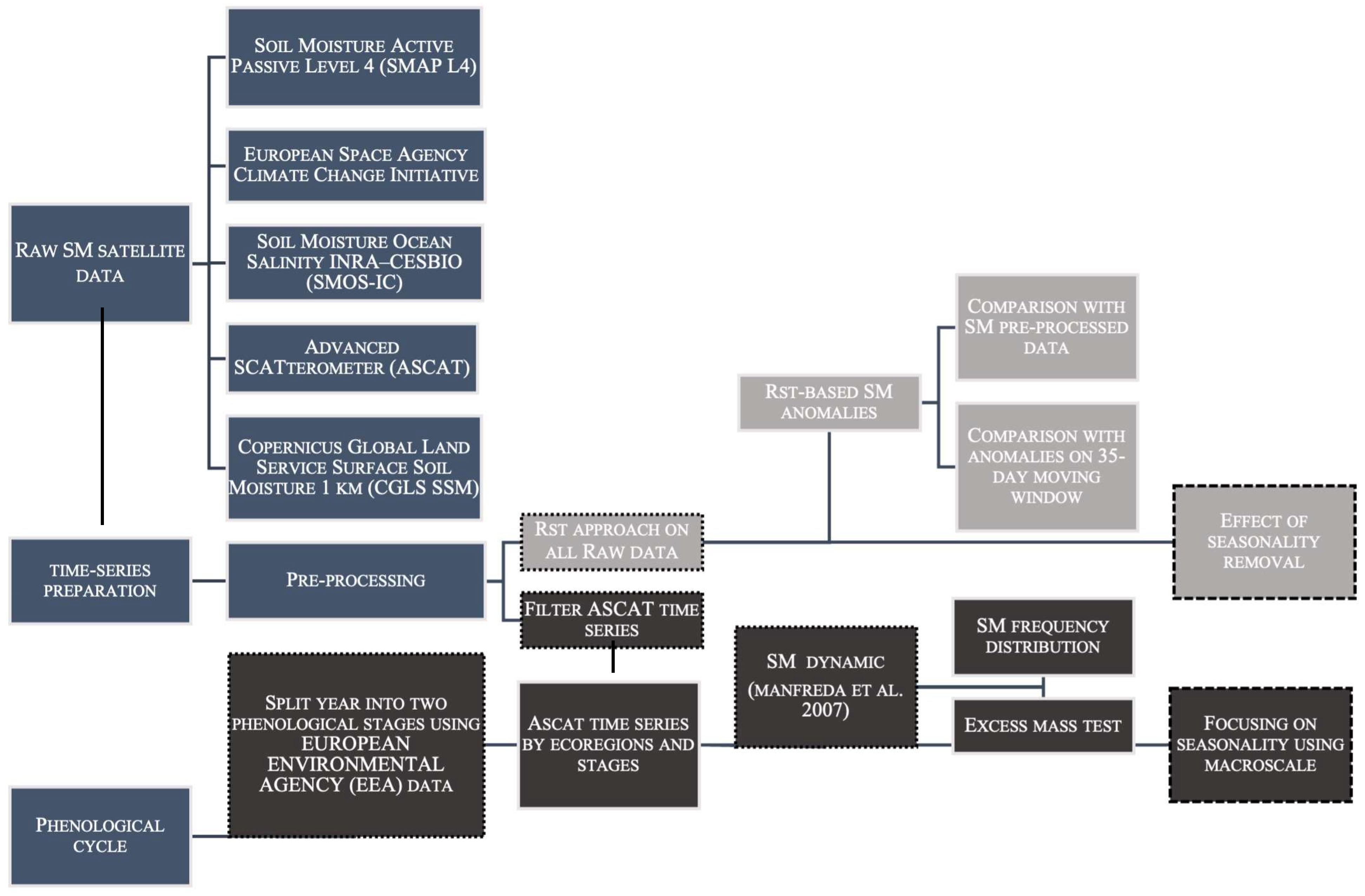
2. Materials and Methods

The impact of seasonality on the SM satellite products considered was investigated by removing it completely, as well as by considering it at two temporal macroscales (i.e., vegetation growth and dormancy phases). Seasonality was eliminated using the Robust Satellite Techniques (RST) approach [23]. After seasonality was removed from the previously examined SM products, the correlation between the long-term anomalies of in situ SM and RS data was evaluated and matched against a similar correlation obtained using a 35-day moving window, as proposed in [24].
In the second phase, we examined the relationship between the vegetation phenological phases and the dynamics of soil wetting/drying at the ecoregion scale. We focused on seasonality (without removal) and considered vegetation to preserve the “memory” of SM.
This allowed us to determine whether combining SM dynamics with large-scale phenological analysis enhanced the RS ability in ecoregion detection. We analyzed the growth and dormancy phases to assess wet or dry soil conditions, factoring in how hydrological processes vary with daily, seasonal, and interannual changes.
The study’s core steps and general workflow (Figure 1) included the following:
  • Data preparation: SM RS data were analyzed against in situ measurements taken within a one-hour time frame and their daily aggregation. The metrics were then computed for each station and aggregated using the ecoregion median, as reported in our previous work [19]. Based on the concept of soil moisture temporal stability [25,26,27], which posits that regional information under certain conditions stores local information, we used the results achieved for the sub-sector (in terms of median values), including the ground stations, as representative of the whole ecoregion, as had been done in the USA [5]. In Section 2.1, the ecoregions considered are highlighted, followed by a brief summary of the ISMN network (Section 2.2) and a presentation of the SM satellite products (Section 2.3).
  • The 35-day moving window and RST anomaly detection approaches are described in detail in Section 2.4.
  • A comparison was made between the RST-based anomalies for each satellite product and both the pre-processed original data and the anomalies derived from a 35-day moving window, with the results detailed in Section 3.1.
  • The identification of vegetation growth and dormancy phases via the European Environment Agency (EEA) data is presented in Section 2.5, and the results of the evaluation of SM dynamics by phases and ecoregions on ASCAT are given in Section 3.2.
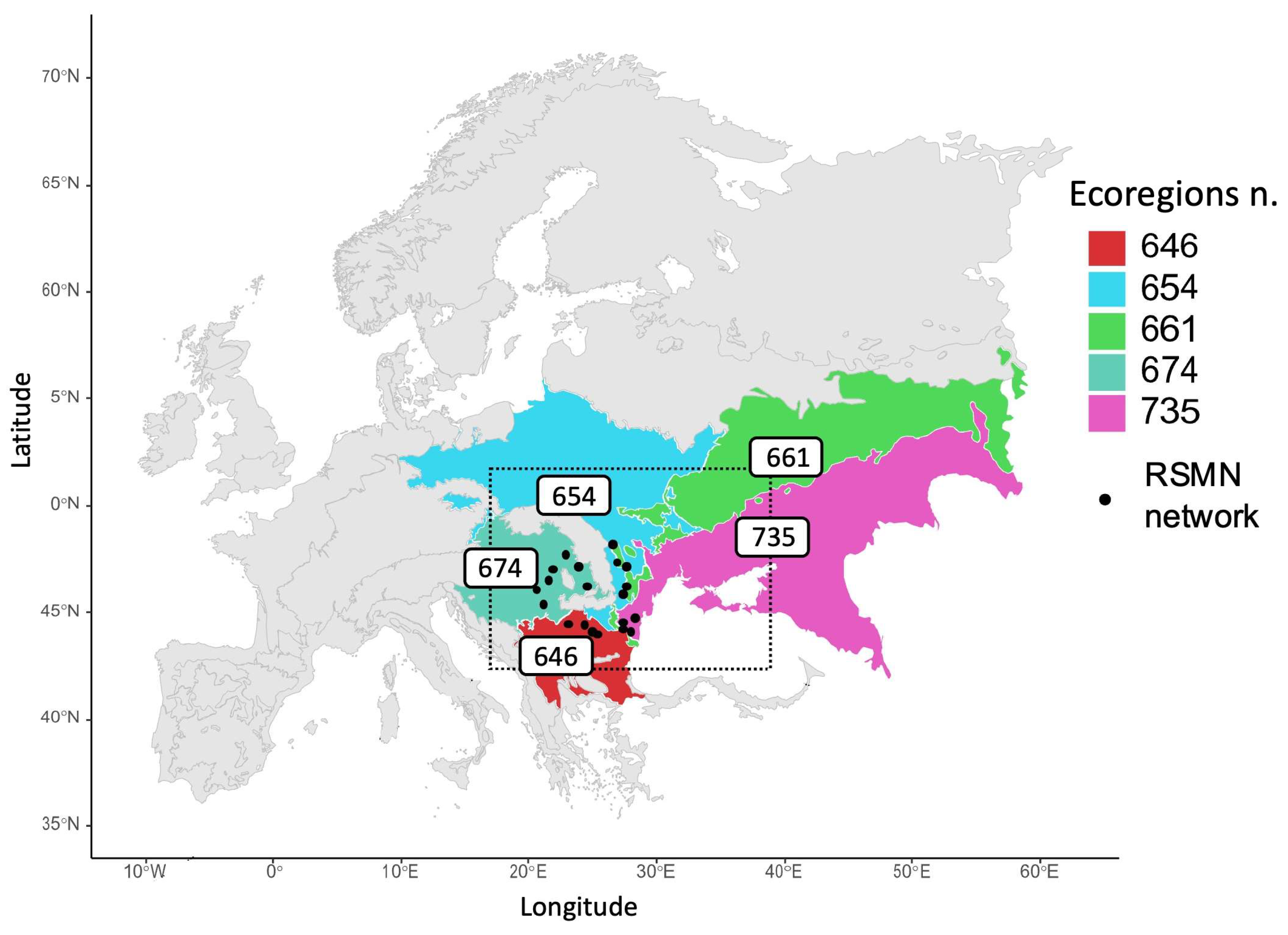
2.1. Study Area

In the Palearctic realm, Europe features six biomes: boreal forests, Mediterranean scrub and woodlands, temperate broadleaf forests, temperate conifer forests, temperate grasslands, and tundra. Within these biomes, there are 37 distinct ecoregions ranging from Mediterranean woodlands to temperate rainforests and tundra.
Each ecoregion has a unique collection of plant and animal species that live together in natural communities [28]. Ecoregions are defined by their natural conditions, such as climate, vegetation, and soil characteristics, and are important for preserving biodiversity [29]. These ecoregions are within Western Eurasia, which includes most of Europe and is the westernmost part of the Palearctic realm. This region is divided into five sub-realms: Greater European Forests, European Mountain Forests, Black Sea Forests and Steppe, the Mediterranean, and the British Isles, encompassing 13 bioregions according to the Bioregions 2020 framework. Among these ecoregions, we are interested in those covered by the Romanian Soil Moisture Network (RSMN):
  • The Balkan mixed forests (unique identification number 646, taken from https://ecoregions.appspot.com/, accessed on 1 November 2022) have high biodiversity and pronounced seasonality, influenced by both Mediterranean and Continental climates.
  • The Central European mixed forests (No. 654) are characterized by a predominantly continental climate.
  • The East European forest steppe (No. 661) is a lowland region extending to the Carpathian foothills in Romania.
  • The Pannonian mixed forests (No. 674) feature extensive grasslands and are bordered by the Carpathian Mountains in the northeast, affecting its climate and reducing central rainfall.
  • The Pontic steppe (No. 735), located in Southeast Romania, experiences a temperate climate with notable winter rainfall.
The subset of European ecoregions representative of the investigated area, as well as the location of the RSMN gauges, are shown in Figure 2.
We chose to focus on these five ecoregions because they showed diverse performance with regard to satellite product predictions of SM in our previous intercomparison [19]. In some ecoregions, all satellite results achieved good performance, whereas in others, no satellite provided good results, although the in situ data were collected under the same network.

2.2. Romanian Soil Moisture Network (RSMN) In Situ Measurements

The satellite products were evaluated using in situ SM measurements from the RSMN taken from January 2015 to December 2020 at a generally assumed sensing depth of 0.05 m [30]. The RSMN is a portion of the ISMN covering Romania. It has been active since 2014, and 20 stations are still running (see Figure 2). The Romanian National Meteorological Administration oversees the RSMN within the scope of the ASSIMO Project (http://assimo.meteoromania.ro/, accessed on 1 November 2022). The network covers the above-mentioned five European ecoregions, each characterized by a different number of stations. Based on the SM temporal stability concept [25,26,27], soil moisture measurements at a local scale can represent wider regions, as the temporal trends of point measurements are closely linked to those of neighboring areas, as demonstrated in the USA [5].

2.3. Satellite SM Products

Several SM products that differed in terms of temporal and spatial resolution, as well as the technology implemented (i.e., passive, active, blended), were analyzed in this study. Their main features are reported in Table 1.
The low spatial resolution SM products used included the following:
  • the SMOS-IC version 02, available at 25 km spatial resolution in both ascending and descending (6:00 a.m./p.m.) orbits;
  • the SMAPL4 v6 model assimilated product (Data Set ID: SPL4SMAU) with a 3 h time resolution on a global 9 km modeling grid;
  • the Metop ASCAT Surface Soil Moisture Climate Data Records, including the H115 Metop ASCAT SSM CDR2019 and its temporal extension H116, at a 12.5 km spatial resolution, converted to volumetric units using a porosity map as in [31];
  • the ESA CCI-SM v06.1 “combined” product at a 0.25° × 0.25° spatial resolution, merging scatterometer-based and radiometer-based soil moisture information.
The high-resolution SM product used was the SSM CGLS 1 km, derived from the Sentinel-1 radar backscatter signal.
A common time frame (i.e., 2015–2020) was selected for this study. As in our previous work [19], we carried out several preprocessing operations. For example, for the H115 and H116 SSM datasets, we excluded values that were less than 0 or exceeded 100, and filtered out data where the processing flags (PROC_FLAG) suggested that retrieval was not completed (e.g., PROC_FLAG > 1), or where the surface state flag (SSF) specified conditions such as unknown, unfrozen, frozen, snow-melting, or permanent ice. For more details on the products and preprocessing workflow, please see [19]. For simplicity, the analysis described in Section 2.5 was performed using H115 and H116 SSM data, which provided SM directly in terms of the degree of saturation, as required for that analysis.

2.4. The Remotion of Short and Long-Term Variation in SM

Calculating long-term SM variation to completely remove seasonality usually requires historical data records spanning several decades [32]. As these data are often unavailable, short-term variations are usually investigated when comparing SM satellite products. One widely recognized approach in the SM community is the use of a moving window, typically spanning several weeks [33,34], computed, for example, as proposed by [35] and applied to the work of [23], as shown in Equation (1):
S M ( t ) A N O M = S M t S M ( t , w ) ¯ s i g m a S M ( t , w )
where SM(t) is the remotely or in situ SM measure acquired at time (t), S M ( t , w ) ¯ is the signal mean soil moisture value computed considering a period from 17 days before (t) to 17 days after (t), and sigmaSM is the relative standard deviation. The computed signal anomaly permits the analysis of short-term variations and minimizes the effect of seasonality.
The quality of SM data can fluctuate significantly with seasons, necessitating temporally adaptive information for many applications. This study aimed to evaluate the performance of SMAP L4, SMOS-IC, ASCAT, ESA CCI, and CGLS SSM 1 km by removing seasonal effects through a method that accounts for long-term variability: the Robust Satellites Technique (RST) approach [23]. The RST is an original and enhanced approach for the long-term statistical analysis of satellite data, which has already proven to be able to furnish valuable insights into SM variability across various spatial and temporal scales using microwave data [9,36,37]. Moreover, it is a versatile satellite data analysis method that has been successfully applied to mitigate various environmental and natural hazards, including those related to the hydrogeological cycle [38,39,40,41,42].
By examining satellite data collected under consistent observational conditions (same location, calendar month, and acquisition times), this technique can discriminate climatological signals from short-term fluctuations, providing a robust identification of signal transients in the investigated dataset from a statistical point of view [23]. The implementation of the RST involves two crucial stages: first, the long-term analysis of the investigated signal to determine its expected value and natural variability, and second, the detection of statistically significant anomalies in the signal through a change-detection analysis. The initial stage requires gathering extensive satellite data over an extended period to ensure uniform conditions at each pixel (x,y). These data were then analyzed to ascertain the normal behavior of the signal, typically expressed as the temporal average and its inherent variability, indicated by the standard deviation. The subsequent stage involves using the Absolute Variation of Local Change of Environment (ALICE) Index to identify statistically significant anomalies in the signal. As proposed by [23], the ALICE Index is calculated as follows in Equation (2):
S M ( x , y , t ) = S M x , y , t S M R E F ( x , y ) σ R E F ( x , y )
where SM is the measurement for each pixel at a particular location (x,y) and time (t); the SMREF and σREF reference values are, respectively, the temporal mean and standard deviation of SM calculated for the same pixel, using data from all the available time series spanning the 2015–2020 period and in the monthly temporal domain. The ALICE index follows a Gaussian distribution in its construction, with a mean of approximately 0 and a standard deviation of approximately 1; therefore, high absolute ALICE values are less likely to occur [36]. We mitigated the negative impact of potential site effects using long-term data acquired under similar climatic conditions. During the creation of the reference fields, values beyond the outer fence (±3IQR) were excluded through quartile analysis for each time series. This methodology was applied to both ISMN ground-based measurements and satellite SM product time series. As for the anomalies detected using the temporal window, the results achieved for each station were aggregated at the ecoregion scale using the median as a reference value. We then calculated the Pearson correlation coefficient, RALICE, and compared it with R and RANOM to evaluate satellite performance in relation to in situ data and both short- and long-term variations.

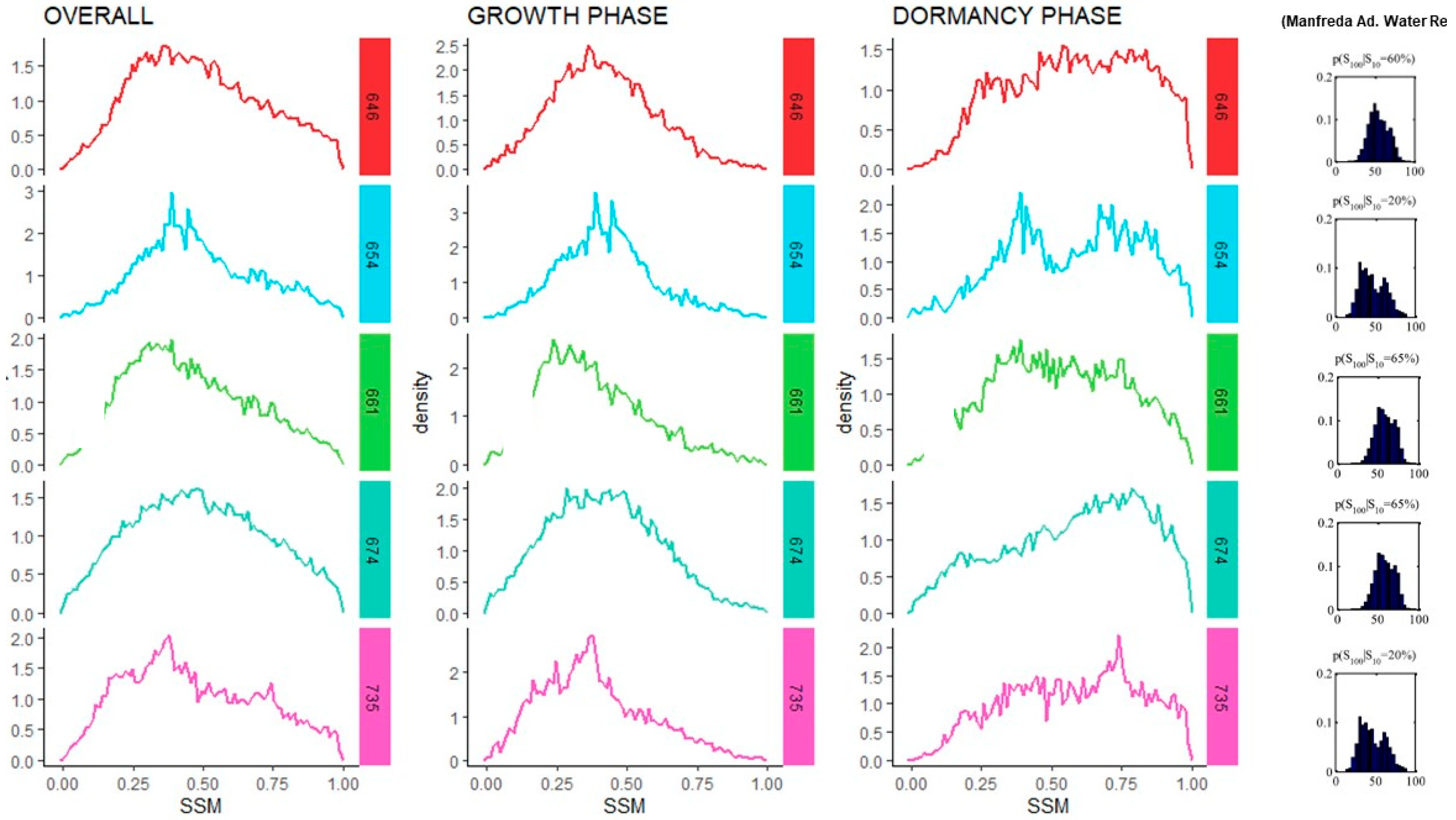
2.5. SM Distribution Analysis Considering the Phenological Cycle

SM is intricately connected to various ecosystem processes and serves as a key indicator of climate and environmental changes [28]. Accordingly, the use of both SM distribution and vegetation phenology can provide a more comprehensive understanding of ecoregions’ seasonality.
We detected plant growth stages by combining data on the start of the vegetation growing season for the 2000–2016 period (https://www.eea.europa.eu/data-and-maps/data/annual-start-of-vegetation-growing, accessed on 1 November 2022) with the length of the growing season for the same period (https://www.eea.europa.eu/data-and-maps/data/annual-above-ground-vegetation-season, accessed on 1 November 2022). The remainder of the year was considered the dormancy phase.
The start of the 2000–2016 growing seasons (SVGS) is represented by a series of daily raster files, categorized by the day of the year (DOY) and their derived linear trends (in days per year). This series uses the Plant Phenology Index (PPI) derived from the MODIS BRDF-Adjusted Reflectance product (MODIS MCD43 NBAR) [43]. The PPI index, optimized for tracking vegetation phenology, is based on MODIS data processed with radiative transfer solutions applied to reflectance in visible-red and near-infrared wavelengths. The MODIS “land” bands (number 1 to 7) data are adjusted using a bidirectional reflectance distribution function to simulate nadir-view conditions, eliminating cross-track illumination effects. The start-of-season indicator is calculated from the annual PPI temporal curve using TIMES AT software for each year between 2000 and 2016. The vegetation growing season length (VGSL) from 2000 to 2016 is a series of raster files showing the annual above-ground growing season length and its linear trends over the same period. PPI is also used to detect the end of the growing season (EOS). We evaluated the satellite SM probability distribution for each ecoregion, considering the entire period and the growth and dormancy phases, based on three soil moisture behaviors (dry/intermediate/wet), as proposed in [22]. The ASCAT SM distributions were tested using the excess mass test, which assumes the multimodality of the distribution as the null hypothesis following the methodology of [42] in the R programming language.
Based on the results obtained by [22], we expected to observe a higher correlation between the surface and root-zone soil moisture when the surface relative saturation assumed values between 0.45 and 0.80 that refers to the so called “intermediate” level soil condition. Therefore, RZSM and SSM may have very low correlations under drier climates. In these ecoregions, deeper microwave penetration should provide insights into the lower soil layers [22]. However, in ecoregions with very wet or intermediate soil conditions, this assumption may not hold. Nonetheless, it is reasonable to expect that the probability distribution of SSM and saturation values would be comparable to that of RZSM because these SM measurements are correlated. Therefore, the surface layer might follow a Gaussian distribution in the case of intermediate-level saturation conditions, whereas under wet conditions, it could exhibit a distribution with significant right-skewness, and we could assume a bimodal distribution under dry soil conditions.

3. Results

To provide an overview of the influence of seasonality removal in SM, we carried out an analysis of the different ecoregions’ performances in terms of the Pearson correlation coefficient (R) between the RS and in situ SM anomalies, as detected by using a 35-day moving window and by using the RST approach. Moreover, the results of this analysis were compared with the case in which seasonality was not removed (Section 3.1).
Having assessed the effectiveness of soil moisture satellite retrievals in raw data and their short- and long-term fluctuations, we then investigated how seasonal changes influence the dynamic patterns of ASCAT SM retrievals. In Section 3.2, we discuss the results of the SM distribution analysis in relation to the phenological cycle.

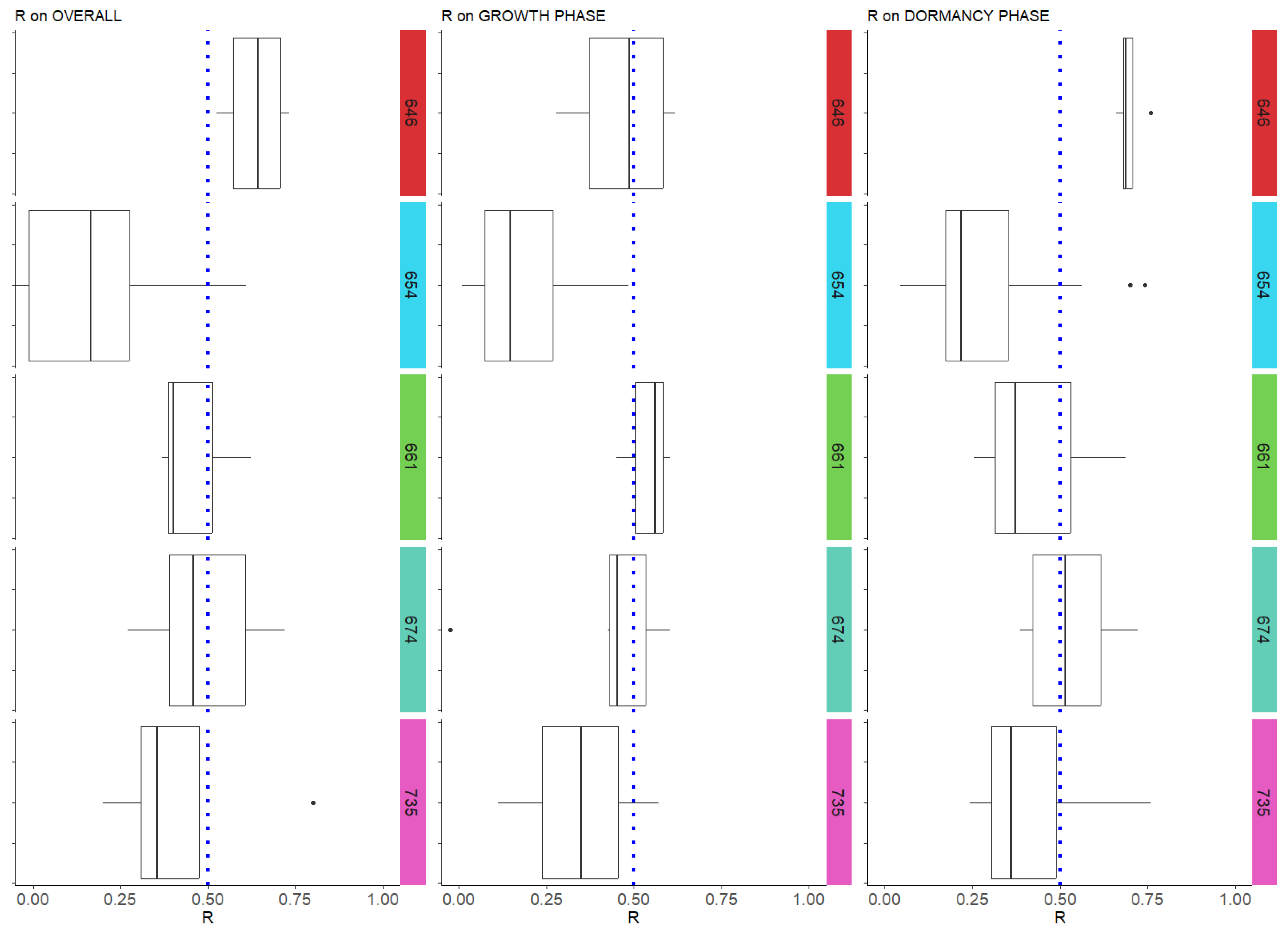
3.1. SM Satellite Comparison in Short- and Long-Term Variation

Table 2 presents a comparison of the performance of the different products by evaluating the Pearson correlation coefficient (R) between in situ SM data and (i) RS data, (ii) short-term anomalies (RANOM) over a 35-day moving window, and (iii) long-term variations RALICE. As previously mentioned, the results for each station were aggregated at the ecoregion scale using the median value as a reference. In Table 2, dark gray highlights ecoregions where a higher correlation was observed when shifting from historical series analysis to anomalies (both ALICE index and 35-day moving window). Such an increase is unexpected because seasonality typically boosts correlation, indicating the sensor/product’s poor ability to detect SM-related signals.
The aim of this study was to determine whether SM satellite performance assessment changed when considering long-term variations (including deviations from the long-term mean seasonal cycle) instead of short-term ones (related to sub-seasonal changes indicating short-term drying and wetting events) in the studied ecoregions.
The results concur with those reported in [19], showing that SMAP L4 was the best performer, followed by ESA CCI, with CGLS performing the worst.
Regarding long-term variations, SMAP L4 and ESA CCI achieved RALICE ≥ 0.5 in two ecoregions, while ASCAT and CGLS did so in one. All four products had RALICE ≥ 0.5 in the Balkan mixed forests (646). SMOS-IC failed to achieve RALICE ≥ 0.5 in any ecoregion. There were additional ecoregions where one satellite achieved a correlation greater than 0.5 (e.g., SMAP L4 in the Central European mixed forests No. 654); however, these cases were unique because R < RALICE.
Both anomaly analyses (i.e., long- and short-term) that aim to remove the effect of seasonality on the SM should reduce the Pearson correlation value between in situ and RS data in the same ecoregion, such that RALICE or RANOM < R. However, a correlation performance inversion (i.e., R < RALICE or R < RANOM), occurred in two regions with SMAP L4 and ESA CCI, and in three regions with ASCAT, CGLS, and SMOS-IC. In all cases, these included the Central European mixed forests (654) and the Pontic steppe (735). The long-term variation enhanced this correlation performance inversion behavior for the active sensors (ASCAT/CGLS), showing R < RALICE, which was not observed in the case of short-term variation, where R continued to exceed RANOM. Considering both R ≥ RANOM and R ≥ RALICE, SMAP L4 and SMOS-IC showed similar performance in describing both short- and long-term variations across ecoregions.
It is interesting to note that the Balkan mixed forests (No. 646) showed strong representation in both short- and long-term variations (R ≥ RALICE and R ≥ RANOM) for all SM satellite products except SMOS-IC, which had RALICE ≥ 0.5. This observation is consistent with another study on the RSMN network [44], which found a high correlation between C-band satellite products like SWI (https://land.copernicus.eu/global/products/swi, accessed on 1 November 2022) and the RSMN network on the Getico Plateau, also in ecoregion No. 646.
Conversely, low correlation values were found near the Romanian Plain and the Dobrogena Plateau, corresponding to the Pontic steppe No. 735 and the Central European mixed forests No. 654. Using the ALICE index for R Pearson evaluation, RALICE confirmed our previous findings reported in [19] and, when compared to short-term variation, showed that in ecoregions 654 and 735, both passive and active sensors (ASCAT/CGLS) demonstrated a higher correlation when transitioning from historical series analysis to anomaly analysis [13]. Such an increase, obtained only using this advanced methodology for multitemporal analysis of satellite data acquired under effectively homogeneous observational conditions, is surprising, as seasonality typically enhances the correlation. Accordingly, its occurrence suggests that these ecoregions are subject to specific conditions.

3.2. Effect Induced by the Phenological Cycle on SM Dynamics

In Section 3.1, we examined the SM products’ behavior by removing seasonality and focusing on SM anomalies. The findings suggested unique hydraulic conditions or effects, such as the presence of subsurface scatterers [45] in ecoregions No. 654 and No. 735. To further explore the role of seasonality, we combined SM distribution data with plant phenological information. As detailed in Section 2.5, we analyzed the growth and dormancy phases for each ecoregion using data from the European Environmental Agency (EEA).
For each RSMN station, we identified phenological stages and calculated the median values aggregated at the ecoregion scale from 2000 to 2016 (Figure 3). Typically, the dormancy phase, where vegetation does not actively use water, corresponds to wetter conditions, while the growth phase is linked to drier periods. We computed the Pearson correlation between SM measurements during these phases for each ground-based station and RS data that were further aggregated at the ecoregion scale, as shown in Figure 4, where the box plots for the ASCAT time series versus in situ measurements are presented for the selected ecoregion.
The correlations were notably higher during the dormancy phase in ecoregions 646 and 674 (Figure 4). For the Balkan mixed forests (646), the correlation increased significantly (mean from 0.5 to 0.7) with reduced variability, as indicated by the closely grouped first and third quartiles in the boxplot. This aligns with the characteristics of the Balkan mixed forests ecoregion No. 646, which experiences considerable seasonal climatic variability, with northern areas characterized by high temperatures and rainfall in June, while the Thracian and Danubian Plains are drier, with some rainfall peaks in early summer and winter (https://www.oneearth.org/ecoregions/balkan-mixed-forests/, accessed on 1 November 2022). This finding suggests a clear connection between phenology and soil moisture variability, which we later combined with soil saturation data to better understand ecoregional behavior.
In Figure 5, we explore SM patterns based on different conditions (dry/intermediate/wet) of the ASCAT time series. This figure illustrates the SM distribution for soil saturation across the overall, growth, and dormancy phases for each ecoregion. From the overall and growth phase distributions, ecoregions No. 646, 661, and 674 generally show Gaussian distributions. In contrast, the Central European mixed forests No. 654 displays bimodal patterns in both graphs. The Pontic steppe No. 735 presents unambiguous characteristics, particularly in terms of the overall SM distribution.
In the dormancy phase (wet conditions), distributions exhibit more variability due to increased water presence across all ecoregions: ecoregions No. 646, 661, and 674 do not show dominant peaks, whereas No. 735 features a peak before reaching 0.75 saturation. Ecoregion 654 maintains a consistent bimodal pattern throughout different phenological stages, indicating clear multimodality with distinct peaks in the dry, wet, and intermediate phases. Comparisons between the growth and dormancy phases reveal consistent multimodal behavior for most ecoregions except the Pontic steppe (735), which shows a large peak at lower values during the growth phase and a large peak at higher values during the dormancy phase. This suggests that overall, the distribution is multimodal. A possible explanation for this multimodal pattern, especially during the dry and growth phases, might be that the satellite measurements reflect deeper soil moisture levels, which differ from the topsoil measurements provided by the ISMN data in this area [13].
Table 3 shows the excess mass test results, which are useful for statistically verifying multimodality [46], estimated by considering the growth and dormancy phases and the whole period. This method focuses on identifying a mode in a frequency distribution by finding a significant excess mass, and the p-value is used for unimodality testing. In the dormancy phase, all ecoregions except 661 exhibited a p-value lower than 0.05; thus, it was easier to find a multimodality pattern even if, in some cases, it was not particularly strong (e.g., in the case of the Pannonian mixed forests).
From the multimodality test, the Central European mixed forests (654) had a strong multimodal distribution in both the growth and dormancy phases (p = 2.20 × 10⁻¹⁶), as did the Pontic steppe (735). However, we cannot reject the null hypothesis for other ecoregions.
These findings indicate that combining SM dynamics with phenology suggests that the difficulties in detecting SM in the Central European mixed forests No. 654 and Pontic steppe No. 735 may not only be due to issues with ground-based measurement stations (e.g., probe calibration and validation problems) as previously proposed in [19]. Instead, these challenges could also arise from prolonged drought conditions where satellite products measure root zone moisture, which differs from the topsoil moisture captured by in situ measurements. This discrepancy is due to the stronger topsoil responses to weather conditions, soil water redistribution, and root water uptake, which reduce the variability in soil moisture and affect its temporal patterns at greater depths. Thus, the way soil moisture patterns change on a seasonal basis (in the case of wetting and drying periods) along the soil profile in different ecoregions can influence the uncertainty of data collected by all SM remote sensing analyses.
Consequently, the approach proposed seems to uncover potential challenges in SM microwave RS at the broader landscape scale.

4. Summary and Conclusions

Owing to the increasing availability of large soil moisture (SM) datasets, several studies have assessed their accuracy at regional/continental scales, obtaining diverse results [13]. To better investigate this lack of coherence, and considering the results achieved in a previous study [19], in this work, we focused on the European ecoregions encompassed by the RSMN network, performing an extensive intercomparison of five SM satellite retrievals, namely SMOS-IC, ASCAT, and CGLS SSM 1 km datasets, as well as including SMAP L4 and the “combined” ESA CCI. To enhance the comparisons reported in [19], we analyzed the main reasons for the miscorrelation and/or great variability in the performance between in situ and satellite SM measurements in this specific area. In particular, we speculated that the miscorrelation could be related to (i) the contribution of seasonality in terms of long-term variation and (ii) the phenological cycle.
It should be noted that there could be additional climatic and physical factors at the origin of this lack of correlation, such as subsurface scatterers, different re-mapping grids of satellite data, and scale discrepancies, that can add uncertainty to the retrieved SM value. However, based on the overall results of the present study, integrating SM dynamics with phenology allowed us to understand that some SM detection issues could arise from specific conditions, such as the occurrence of prolonged drought phases. This is an important update compared to [19], where the authors suggested that the unique issue was related to the ground-based measurement stations.
In more detail, the results clearly indicate that when a long-term analysis is conducted, it is essential to remove the seasonality contribution to obtain a more robust view of performance. Moreover, more advanced methods, such as Robust Satellite Techniques, should be used to effectively remove both long- and short-term seasonal effects. This is the first relevant result that should be taken into account by the scientific community to allow for the homogenization of protocols and guidelines for analyzing soil moisture datasets.
Using vegetation phenology coupled with SM frequency distribution can allow for a better understanding of the low level of correlation between in situ and satellite measurements in some specific areas. The incorporation of plant phenology, focusing on the growth and dormancy phases, was essential for understanding SM distribution patterns and assessing the subregions with less accuracy that were characterized by very long drying periods. Therefore, future studies aimed at analyzing soil moisture behavior at a landscape scale should consider vegetation presence and its phenological cycle to determine the complex dependence of localized soil moisture on site-specific land surface properties that often affect in situ data.
Finally, it is worth mentioning that the presence of very dry soil can negatively affect the level of correlation between in situ and remotely measured SM data, due to the different depths to which these measurements refer. This condition will be more prevalent in the future because of climate change; therefore, these data need to be used with caution, with efforts to harmonize measurement depth, potentially moving from surface SM to root zone SM. This aspect will be the main topic of future work by the authors.

Author Contributions

Conceptualization, R.A.; Methodology, R.A. and A.M.; Validation, A.M.; Formal analysis, T.L. and A.M.; Data curation, T.L. and A.M.; Writing—original draft, R.A. and A.M.; Writing—review & editing, R.A., T.L., S.M. and J.A.; Visualization, S.M., J.A. and A.S.; Supervision, R.A. and A.S. All authors have read and agreed to the published version of the manuscript.

Funding

This research received no external grant.

Data Availability Statement

The raw data supporting the conclusions of this article will be made available by A.M. on request. The input data used in this study are mostly freely available on the web and the data information are provided in the text or web-link is provided.

Acknowledgments

The content of this manuscript is part of the study proposed in the PhD thesis of A.M. under the supervision of R.A. and A.S. and, therefore, some concepts, results, figures or tables could be derived or adapted from it.

Conflicts of Interest

The authors declare no conflict of interest.

References

  1. Luo, M.; Meng, F.; Sa, C.; Duan, Y.; Bao, Y.; Liu, T.; Maeyer, P.D. Response of vegetation phenology to soil moisture dynamics in the Mongolian Plateau. CATENA 2021, 206, 105505. [Google Scholar] [CrossRef]
  2. Albano, R.; Manfreda, S.; Celano, G. MY SIRR: Minimalist agro-hYdrological model for Sustainable IRRigation management—Soil moisture and crop dynamics. SoftwareX 2017, 6, 107–117. [Google Scholar] [CrossRef]
  3. Entin, J.K.; Robock, A.; Vinnikov, K.Y.; Hollinger, S.E.; Liu, S.; Namkhai, A. Temporal and spatial scales of observed soil moisture variations in the extratropics. J. Geophys. Res. 2000, 105, 11865–11877. [Google Scholar] [CrossRef]
  4. Li, B.; Rodell, M. Spatial variability and its scale dependency of observed and modeled soil moisture over different climate regions. Hydrol. Earth Syst. Sci. 2013, 17, 1177–1188. [Google Scholar] [CrossRef]
  5. Baldwin, D.; Manfreda, S.; Keller, K.; Smithwick, E.A.H. Predicting root zone soil moisture with soil properties and satellite near-surface moisture data across the conterminous United States. J. Hydrol. 2017, 546, 393–404. [Google Scholar] [CrossRef]
  6. Scipal, K.; Scheffler, C.; Wagner, W. Soil moisture runoff relation at the catchment scale as observed with coarse resolution microwave remote sensing, Hydrology and Earth Syst. Sciences 2005, 9, 173–183. [Google Scholar] [CrossRef]
  7. Scipal, K.; Drusch, M.; Wagner, W. Assimilation of a ERS scatterometer derived soil moisture index in the ECMWF numerical weather prediction system. Adv. Water Resour. 2008, 31, 1101–1112. [Google Scholar] [CrossRef]
  8. Albergel, C.; Rüdiger, C.; Carrer, D.; Calvet, J.-C.; Fritz, N.; Naeimi, V.; Bartalis, Z.; Hasenauer, S. An evaluation of ASCAT surface soil moisture products with in-situ observations in southwestern France. Hydrol. Earth Syst. Sci. 2009, 13, 115–124. [Google Scholar] [CrossRef]
  9. Lacava, T.; Brocca, L.; Calice, G.; Melone, F.; Moramarco, T.; Pergola, N.; Tramutoli, V. Soil moisture variations monitoring by AMSU-based soil wetness indices: A long-term inter-comparison with ground measurements. Remote Sens. Environ. 2010, 114, 2317–2325. [Google Scholar] [CrossRef]
  10. Gruber, A.; De Lannoy, G.; Albergel, C.; Al-Yaari, A.; Brocca, L.; Calvet, J.-C.; Colliander, A.; Cosh, M.; Crow, W.; Dorigo, W.; et al. Validation practices for satellite soil moisture retrievals: What are (the) errors? Remote Sens. Environ. 2020, 244, 111806. [Google Scholar] [CrossRef]
  11. Chakravorty, A.; Chahar, B.R.; Sharma, O.P.; Dhanya, C.T. A regional scale performance evaluation of SMOS and ESA-CCI soil moisture products over India with simulated soil moisture from MERRA-Land. Remote Sens. Environ. 2016, 186, 514–527. [Google Scholar] [CrossRef]
  12. Van der Schalie, R.; De Jeu, R.; Rodríguez-Fernández, N.; Al-Yaari, A.; Kerr, Y.; Wigneron, J.-P.; Parinussa, R.; Drusch, M. The effect of three different data fusion approaches on the quality of soil moisture retrievals from multiple passive microwave sensors. Remote Sens. 2018, 10, 107. [Google Scholar] [CrossRef]
  13. Mazzariello, A. A Four-Dimensional Soil Moisture Product: Closing the Soil Profile Gap with a SWI-SMAR Approach. Ph.D. Thesis, University of Basilicata, Potenza, Italy, 26 February 2024. [Google Scholar]
  14. Gruber, A.; Scanlon, T.; van der Schalie, R.; Wagner, W.; Dorigo, W. Evolution of the ESA CCI Soil Moisture climate data records and their underlying merging methodology. Earth Syst. Sci. Data 2019, 11, 717–739. [Google Scholar] [CrossRef]
  15. Kim, H.; Crow, W.T.; Wagner, W.; Li, X.; Lakshmi, V. A Bayesian machine learning method to explain the error characteristics of global-scale soil moisture products. Remote Sens. Environ. 2023, 296, 113718. [Google Scholar] [CrossRef]
  16. Haugaasen, T.; Peres, C.A. Primate assemblage structure in Amazonian flooded and unflooded forests. Am. J. Primatol. 2005, 67, 243–258. [Google Scholar] [CrossRef]
  17. Keenan, T.F.; Gray, J.; Friedl, M.A.; Toomey, M.; Bohrer, G.; Hollinger, D.Y.; Munger, J.W.; O’Keefe, J.; Schmid, H.P.; Wing, I.S. Net carbon uptake has increased through warming-induced changes in temperate forest phenology. Nat. Clim. Chang. 2014, 4, 598–604. [Google Scholar] [CrossRef]
  18. Myneni, R.B.; Keeling, C.; Tucker, C.J.; Asrar, G.; Nemani, R.R. Increased plant growth in the northern high latitudes from 1981 to 1991. Nature 1997, 386, 698–702. [Google Scholar] [CrossRef]
  19. Mazzariello, A.; Albano, R.; Lacava, T.; Manfreda, S.; Sole, A. Intercomparison of recent microwave satellite soil moisture products on European ecoregions. J. Hydrol. 2023, 626, 130311. [Google Scholar] [CrossRef]
  20. Rodriguez-Iturbe, I.; Porporato, A.; Ridolfi, L.; Isham, V.M.; Coxi, D.R. Probabilistic modelling of water balance at a point: The role of climate, soil and vegetation. Proc. R. Soc. Lond. A 1999, 455, 3789–3805. [Google Scholar] [CrossRef]
  21. Laio, F.; Porporato, A.; Ridolfi, L.; Rodriguez-Iturbe, I. Plants in water-controlled ecosystems: Active role in hydrologic processes and response to water stress: II. Probabilistic Soil Moisture Dyn. Adv. Water Resour. 2001, 24, 707–723. [Google Scholar] [CrossRef]
  22. Manfreda, S.; McCabe, M.F.; Fiorentino, M.; Rodríguez-Iturbe, I.; Wood, E.F. Scaling characteristics of spatial patterns of soil moisture from distributed modelling. Adv. Water Resour. 2007, 30, 2145–2150. [Google Scholar] [CrossRef]
  23. Tramutoli, V. Robust AVHRR Techniques (RAT) for environmental monitoring: Theory and applications. In Proceedings of the Earth Surface Remote Sensing II, Barcelona, Spain, 21–24 September 1998; pp. 101–113. [Google Scholar]
  24. Brocca, L.; Hasenauer, S.; Lacava, T.; Melone, F.; Moramarco, T.; Wagner, W.; Dorigo, W.; Matgen, P.; Martínez-Fernández, J.; Llorens, P.; et al. Soil moisture estimation through ASCAT and AMSR-E sensors: An intercomparison and validation study across Europe. Remote Sens. Environ. 2011, 115, 3390–3408. [Google Scholar] [CrossRef]
  25. Brocca, L.; Melone, F.; Moramarco, T.; Morbidelli, R. Soil moisture temporal stability over experimental areas in Central Italy. Geoderma 2009, 148, 364–374. [Google Scholar] [CrossRef]
  26. Cosh, M.H.; Jackson, T.J.; Starks, P.; Heathman, G. Temporal stability of surface soil moisture in the Little Washita River watershed and its applications in satellite soil moisture product validation. J. Hydrol. 2006, 323, 168–177. [Google Scholar] [CrossRef]
  27. Starks, P.J.; Heathman, G.C.; Jackson, T.J.; Cosh, M.H. Temporal stability of soil moisture profile. J. Hydrol. 2006, 324, 400–411. [Google Scholar] [CrossRef]
  28. Berra, E.F.; Gaulton, R. Remote sensing of temperate and boreal forest phenology: A review of progress, challenges and opportunities in the intercomparison of in-situ and satellite phenological metrics. For. Ecol. Manag. 2021, 480, 118663. [Google Scholar] [CrossRef]
  29. Omernik, J.M.; Griffith, G.E. Ecoregions of the conterminous United States: Evolution of a hierarchical spatial framework. Environ. Manag. 2014, 54, 1249–1266. [Google Scholar] [CrossRef]
  30. Sayre, R.; Dangermond, J.; Frye, C.; Vaughan, R.; Aniello, P.; Breyer, S.; Cribbs, D.; Hopkins, D.; Nauman, R.; Derrenbacher, W.; et al. A New Map of Global Ecological Land Units—An Ecophysiographic Stratification Approach; Association of American Geographers: Washington, DC, USA, 2014; Volume 46. [Google Scholar]
  31. Gleeson, T.; Moosdorf, N.; Hartmann, J.; van Beek, L.P.H. A glimpse beneath earth’s surface: GLobal HYdrogeology MaPS (GLHYMPS) of permeability and porosity. Geophys. Res. Lett. 2014, 41, 3891–3898. [Google Scholar] [CrossRef]
  32. Dorigo, W.; De Jeu, R.; Chung, D.; Parinussa, R.; Liu, Y.; Wagner, W.; Fernández-Prieto, D. Evaluating global trends (1988–2010) in harmonized multi-satellite surface soil moisture. Geophys. Res. Lett. 2012, 39, L18405. [Google Scholar] [CrossRef]
  33. Albergel, C.; De Rosnay, P.; Gruhier, C.; Muñoz-Sabater, J.; Hasenauer, S.; Isaksen, L.; Kerr, Y.; Wagner, W. Evaluation of remotely sensed and modelled soil moisture products using global ground-based in situ observations. Remote Sens. Environ. 2012, 118, 215–226. [Google Scholar] [CrossRef]
  34. Chen, F.; Crow, W.T.; Colliander, A.; Cosh, M.H.; Jackson, T.J.; Bindlish, R.; Reichle, R.H.; Chan, S.K.; Bosch, D.D.; Starks, P.J.; et al. Application of Triple Collocation in Ground-Based Validation of Soil Moisture Active/Passive (SMAP) Level 2 Data Products. IEEE J. Sel. Top. Appl. Earth Obs. Remote Sens. 2017, 10, 489–502. [Google Scholar] [CrossRef]
  35. Rodríguez-Fernandez, N.; Kerr, Y.; van der Schalie, R.; Al-Yaari, A.; Wigneron, J.-P.; de Jeu, R.; Richaume, P.; Dutra, E.; Mialon, A.; Drusch, M. Long Term Global Surface Soil Moisture Fields Using an SMOS-Trained Neural Network Applied to AMSR-E Data. Remote Sens. 2016, 8, 959. [Google Scholar] [CrossRef]
  36. Lacava, T.; Greco, M.; Di Leo, E.; Martino, G.; Pergola, N.; Romano, F.; Sannazzaro, F.; Tramutoli, V. Assessing the potential of SWVI (Soil Wetness Variation Index) for hydrological risk monitoring by means of satellite microwave observations. Adv. Geosci. 2005, 2, 221–227. [Google Scholar] [CrossRef]
  37. Manfreda, S.; Lacava, T.; Onorati, B.; Pergola, N.; Di Leo, M.; Margiotta, M.R.; Tramutoli, V. On the use of AMSU-based products for the description of soil water content at basin scale. Hydrol. Earth Syst. Sci. 2011, 15, 2839–2852. [Google Scholar] [CrossRef]
  38. Lahsaini, M.; Albano, F.; Albano, R.; Mazzariello, A.; Lacava, T. A Synthetic Aperture Radar-Based Robust Satellite Technique (RST) for Timely Mapping of Floods. Remote Sens. 2024, 16, 2193. [Google Scholar] [CrossRef]
  39. Di Polito, C.; Ciancia, E.; Coviello, I.; Doxaran, D.; Lacava, T.; Pergola, N.; Satriano, V.; Tramutoli, V. On the Potential of Robust Satellite Techniques Approach for SPM Monitoring in Coastal Waters: Implementation and Application over the Basilicata Ionian Coastal Waters Using MODIS-Aqua. Remote Sens. 2016, 8, 922. [Google Scholar] [CrossRef]
  40. Lacava, T.; Filizzola, C.; Pergola, N.; Sannazzaro, F.; Tramutoli, V. Improving flood monitoring by the Robust AVHRR Technique (RAT) approach: The case of the April 2000 Hungary flood. Int. J. Remote Sens. 2010, 31, 2043–2062. [Google Scholar] [CrossRef]
  41. Lacava, T.; Ciancia, E.; Faruolo, M.; Pergola, N.; Satriano, V.; Tramutoli, V. On the Potential of RST-FLOOD on Visible Infrared Imaging Radiometer Suite Data for Flooded Areas Detection. Remote Sens. 2019, 11, 598. [Google Scholar] [CrossRef]
  42. Satriano, V.; Ciancia, E.; Filizzola, C.; Genzano, N.; Lacava, T.; Tramutoli, V. Landslides Detection and Mapping with an Advanced Multi-Temporal Satellite Optical Technique. Remote Sens. 2023, 15, 683. [Google Scholar] [CrossRef]
  43. Jin, H.; Eklundh, L. A physically based vegetation index for improved monitoring of plant phenology. Remote Sens. Environ. 2014, 152, 512–525. [Google Scholar] [CrossRef]
  44. Ontel, I.; Irimescu, A.; Boldeanu, G.; Mihailescu, D.; Angearu, C.-V.; Nertan, A.; Craciunescu, V.; Negreanu, S. Assessment of Soil Moisture Anomaly Sensitivity to Detect Drought Spatio-Temporal Variability in Romania. Sensors 2021, 21, 8371. [Google Scholar] [CrossRef] [PubMed]
  45. Naeimi, V.; Paulik, C.; Bartsch, A.; Wagner, W.; Kidd, R.; Park, S.-E.; Elger, K.; Boike, J. ASCAT Surface State Flag (SSF): Extracting information on surface freeze/thaw conditions from backscatter data using an empirical threshold-analysis algorithm. IEEE Trans. Geosci. Remote Sens. 2012, 50, 2566–2582. [Google Scholar] [CrossRef]
  46. Ameijeiras-Alonso, J.; Crujeiras, R.M.; Rodríguez-Casal, A. Mode testing, critical bandwidth and excess mass. Test 2019, 28, 900–919. [Google Scholar] [CrossRef]
Figure 1. General study workflow: the blue boxes indicate pre-processing phases, and the grey and dark gray boxes indicate the steps related to the ALICE index and the phenological seasonality and dynamic behavior of soil moisture (SM), respectively. The figure is adapted from [13]. Please note that the “SM Dynamic” analysis refers to the work of Manfreda et al., 2007 in [22].
Remotesensing 16 03044 g001
Figure 2. Ecoregions analyzed in the present study and the Romanian Soil Moisture Network (RSMN).
Remotesensing 16 03044 g002
Figure 3. Growth (blue) and dormancy (light gray) phases in each ecoregion. Derived from [13].
Remotesensing 16 03044 g003
Figure 4. Pearson Correlation Coefficient between ASCAT time series and in situ ISMN boxplots for the following ecoregions: No. 646 Balkan mixed forests, No. 654 Central European mixed forests, No. 661 East European forest steppe, No. 674 Pannonian mixed forests, and No. 735 Pontic steppe. Derived from [13].
Remotesensing 16 03044 g004
Figure 5. Overall, the growth phase and dormancy phase surface soil moisture (SSM) frequency distribution in the Balkan mixed forests (646), Central European mixed forests (654), East European forest steppe (661), Pannonian mixed forests (674), and Pontic steppe (735). N.B. A different maximum y-value was employed depending on the sample distribution in order to avoid losing details of the curve shape. Adapted from [13].
Remotesensing 16 03044 g005
Table 1. Main features of the SM satellite products.
AcronymTypeVersionUnitsTemporal Resolution (Acquisition Time,
When Available)
Spatial Sampling
SMOSPassiveSMOS-ICm3/m312 h
(6:00 a.m./p.m.)
25 km
SMAPPassive, model-basedSMAP L4 V5m3/m33 h9 km
ASCATActiveH115 and H116% (degree of saturation)12 h
(9:30 a.m./p.m.)
12.5 km
CGLSActiveSSM—1 km V1% (degree of saturation)1.5–4 days1 km
ESA CCICombinedESA CCI v06.1m3/m3Daily0.25°
Table 2. Comparison of R, RANOM, and RALICE as derived from [13].
ASCATCGLSESA CCISMAPL4SMOS-IC
EcoregionsRRANOMRALICERRANOMRALICERRANOMRALICERRANOMRALICERRANOMRALICE
6460.6420.4060.5050.5760.4160.5250.6580.4840.5680.7110.5470.5760.5870.3500.440
6540.1890.3590.3140.1640.2700.2600.0450.3130.3670.3430.5460.5000.1770.4710.336
6610.3990.4830.4230.2800.4590.4680.4810.4810.5010.5800.4900.4600.2730.3760.358
6740.4580.4160.4090.4560.3990.4230.4900.4480.4700.5390.5060.4950.3790.3110.325
7350.3550.2200.4160.3420.1060.4670.3470.4260.4570.3130.3860.4620.2610.3800.379
Median0.3990.4060.4160.3420.3990.4670.4810.4480.4700.5390.5060.4950.2730.3760.358
Table 3. Overall multimodality and multimodality test by stage for the five ecoregions as derived from [13].
Ecoregionsp-Value
OverallGrowth
Phase
Dormancy
Phase
6460.2440.0682.20 × 10−16
6542.20 × 10−162.20 × 10−162.20 × 10⁻¹⁶
6610.0740.0080.096
6740.0320.0020.014
7352.20 × 10−160.0022.20 × 10−16
Disclaimer/Publisher’s Note: The statements, opinions and data contained in all publications are solely those of the individual author(s) and contributor(s) and not of MDPI and/or the editor(s). MDPI and/or the editor(s) disclaim responsibility for any injury to people or property resulting from any ideas, methods, instructions or products referred to in the content.

