A Multi-Objective Intelligent Optimization Method for Sensor Array Optimization in Distributed SAR-GMTI Radar Systems

Abstract

The design and optimization of sensor array configurations is a significant challenge for distributed SAR-GMTI radar systems because the system performance of distributed array radar is a comprehensive result of several conflicting evaluation indicators. This paper developed a multi-objective intelligent optimization method to solve the global optimal problem of array configurations in terms of achieving optimal GMTI performance. Firstly, to formulate the relationship between array configuration and GMTI performance, we established three objective functions derived from evaluating indicators of SAR-GMTI performance. Specifically, in the objective functions, we proposed a novel clutter covariance matrix model that added several typical non-ideal factors of the real-world detection environment. This provides a way to build a bridge between the array configuration, environment clutter, and GMTI performance. Then, we proposed an improved multi-objective snake optimization algorithm (IMOSOA) that combined the Pareto optimization mechanism with snake optimization to solve the multi-objective optimization problem while reconciling the conflicts between different objective functions. Meanwhile, some significant improvements were made to speed up convergence. That is, tent chaotic mapping-based initialization, multi-group coevolution, and individual mutation strategies were applied to solve the non-convergence problem of global searching. Finally, in the case of an airborne SAR-GMTI system, numerical experiments demonstrated that the proposed IMOSOA has superior performance than other contrast methods, especially in terms of GMTI applications.

1. Introduction

Ground moving target indication (GMTI) is of great significance for spaceborne/airborne synthetic aperture radar (SAR) surveillance systems [1,2]. Distributed SAR-GMTI radar has superior performance in target positioning, slowly moving target indication, and parameter estimation, benefiting from the large size of the antenna aperture [3,4]. Especially for airborne distributed array radar, there is sufficient physical space to enlarge the radar antenna aperture on the carrier platform. Thus, it has great potential in SAR-GMTI applications. However, distributed array radar is confronted with the following three difficult problems that result in system performance degradation. First, a spatially sparse array gives rise to the grating lobe antenna pattern [5]. This leads to blind speed for moving target detection and increases interference from the grating lobe. Second, a non-ideal linear array configuration (caused by the irregular surface of the fuselage or the circular orbital configuration of satellites) will bring about a hybrid baseline, including along-track and cross-track baselines. This results in cluttered statistical distribution properties that change with range and terrain elevation, thereby leading to deterioration of the clutter suppression ability [6,7]. Third, the GMTI performance indicators, minimum detectable velocity (MDV) and blind speed, strongly rely on the configuration of sub-arrays [8]. In brief, the aforementioned three problems are coupled with array configuration. Consequently, the optimization of sub-array configuration is of great significance for GMTI applications in distributed array radar systems.

To cope with the first problem, a popular and effective approach is sparse array optimization [9,10,11,12,13]. In the past decades, scholars have made great progress in optimization methods for sparse array designs. They take the array position as the optimization object for the purpose of reducing the peak side lobe level of the antenna pattern or optimum beamforming. And the final sub-array arrangement can be obtained through optimization algorithms, including convex optimization [14,15], compressed sensing [16], intelligent optimization algorithms [17,18], etc. It is commonly known that solving sub-array arrangement is a non-convex intractable problem. To improve the time efficiency of global search processes, scholars have applied numerous intelligent biomimetic algorithms in the field of sparse array optimization, such as the genetic algorithm [19,20], ant colony optimization [21,22], particle swarm optimization [23,24], firefly algorithm [25], and their improved algorithms, which have been applied for antenna array optimization and obtained outstanding achievements [26,27].

As is well known, the indicators of pattern response are incompatible. Thus, it has little significance if only the peak side lobe level is improved. To address this issue, researchers have introduced multi-objective optimization technology to span array synthesis [28,29]. They proposed the multi-objective optimization algorithm through designing multiple optimization objectives, such as strong directional pencil beams, low side lobe level, and cross polarization suppression. But the other difficulty is how to obtain the global optimal solution while balancing the contradiction between multi-objectives. On this issue, many scholars have combined existing bionic algorithms with Pareto optimization [30,31]. The typical intelligent biomimetic methods include the second generation non-dominated sorting genetic algorithm (NSGA-II) [32], the multi-objective artificial bee colony algorithm (MOABC) [33], the multi-objective ant lion optimizer (MOALO) algorithm [34], the multi-objective butterfly optimization algorithm (MOBOA) [35], and the multi-objective salp swarm algorithm (MOSSA) [36]. They have been proven to have outstanding performance with the advantages of diverse populations, few parameters, and fast speed of convergence. However, with the increase in array aperture or elements, the computation cost will greatly increase, and the phenomenon of “prematurity” tends to appear.

For the second problem, space–time adaptive processing (STAP) technology has demonstrated good performance in GMTI applications for spaceborne/airborne SAR-GMTI radar [37,38,39]. Scholars have developed many methods to improve STAP performance. They proposed the sample selection method and sample weighting method for improving the estimation accuracy of the clutter covariance matrix (CCM) under a nonhomogeneous clutter background [40,41]. Knowledge-aided STAP (KA-STAP) can largely improve the performance of clutter cancelation by using prior information to reconstruct the CCM [42,43]. The sparse recovery-based STAP (SR-STAP) method can essentially solve the problem of clutter spectrum estimation [44]. But it also faces some challenges in real-world engineering applications, i.e., large computation. In our previous work, we proposed several new methods for clutter compensation and sample selecting that work for hybrid baseline radar systems [6,7]. All of these methods have proven the superiority of GMTI performance. However, sub-array configuration is still the most fundamental factor that directly restricts the clutter distribution property and determines the GMTI performance of distributed array radar systems.

For the aforementioned three problems, the ultimate goal of array optimization is to improve GMTI performance. This is a comprehensive result that includes multiple influencing factors, including antenna pattern synthesis, STAP filtering response, clutter suppression capability, target blind speed, etc. Therefore, the optimization of sub-array configurations for optimal GMTI performance should be a multi-objective optimization problem (MOP).

Although there are many excellent studies focused on sparse array optimization, comprehensive array optimization for improving the GMTI performance of the system has not previously appeared. In other words, it is a significant challenge for radar system designers to design an array configuration to obtain optimal GMTI performance with multiple influencing factors taken into consideration. Therefore, this paper focuses on the optimization of sub-array arrangement for GMTI applications in the case of spaceborne/airborne distributed array radar systems. We propose an improved multi-objective snake optimization algorithm (IMOSOA) for the problem of global optimal array configuration design in distributed SAR-GMTI radar systems. The main contributions of IMOSOA can be summarized as follows:

• We established a functional model to describe the influence of array configuration on GMTI performance based on the CCM model and SCNR-Loss model. It provides a way to build a bridge between the array configuration, the non-ideal factors of the detection environment, and the GMTI performance of distributed radar.
• We proposed a multi-objective optimization problem for array arrangement design. Three objective functions were derived corresponding to three indicators of SAR-GMTI performance, including the width of the filtering “notch” (or MDV), the magnitude of the clutter suppression ability, and the probability of target blind speed. It provides a fresh idea for radar system performance optimization.
• We introduced the Pareto optimization mechanism to solve MOP. This approach can balance the conflicts between different objective functions (or GMTI performance indicators) and improve at least one indicator while not worsening the other criteria.
• To improve the optimal solution as well as speed up the convergence of the snake optimization algorithm, an improved method, IMOSOA, was proposed for the initialization and evolutionary process. That is, we introduced tent chaotic mapping to generate initial solutions, applied the multi-group cooperative strategy to increase population diversity, and increased the probability of individual mutation to reduce the risk of local convergence.

The remainder of this paper is organized as follows. Section 2 gives the geometric and signal model of distributed array radar and presents related works of multi-objective optimization and the snake optimization algorithm. Section 3 describes the principle and procedure of the proposed IMOSOA, including the method of CCM construction, the definition of three objective functions, and the improvement strategies of IMOSOA. Section 4 shows the experimental results and provides the comparative analysis to prove the advantages of the proposed method. Finally, Section 5 gives the conclusions and prospects.

2. Signal Model and Problem Statement

2.1. Signal Model of Distributed Array Radar

2.1.1. Geometry Model

Spaceborne/airborne distributed array radar usually generates a non-ideal linear array configuration due to satellite formation flight or the irregular surface of the fuselage. The geometric model of the satellite orbit is a parameterized ellipse, but a model of the fuselage is relatively complex. Thus, this paper pays more attention to airborne distributed array radar systems. According to the investigation of fuselage aerodynamic structure characteristics [45], the geometric model of the fuselage side and tail can be fitted as two ellipses. A geometric diagram of distributed array radar is illustrated in Figure 1.

Without loss of generality, we established a Cartesian coordinate that the x-axis points in the flight direction of the carrier platform; the y-axis is parallel to the aircraft wing; and the positive direction of the z-axis satisfies the right-hand rule. On this basis, the side and tail parts of the fuselage were modeled as two short arc segments from two ellipses for which the short axes overlapped on the y-axis.

To balance the coverage of detection range and the accuracy of target velocity estimation and positioning in SAR-GMTI applications, the distributed array radar adopts a single-transmit multiple-receiver mode. Without loss of generality, we assume that all sub-arrays are planar arrays and work in side-looking mode. The position vector of the n-th sub-array on the side of fuselage can be represented as follows:

$$p_n=\left[\begin{array}{c}{x}_n\\ y_n\\ z_n\end{array}\right]=\left\{\begin{array}{c}{a}_{bo}\cos {\theta }_n\\ b_{bo}\sin {\theta }_n-b_{bo}\\ 0\end{array}\right\}$$

(1)

where $a_{bo}$ and $b_{bo}$ represent the major and minor axes of the ellipse $O_{bo}$, respectively, and ${\theta }_n$ denotes the centrifugal angle of the $n$-th sub-array.

Similarly, the position vector of the $m$-th sub-array arranged in the tail area can be expressed as follows:

$$p_m=\left[\begin{array}{c}{x}_m\\ y_m\\ z_m\end{array}\right]=\left\{\begin{array}{c}{a}_{ta}\cos {\theta }_m\cos {\theta }_e\\ b_{ta}\sin {\theta }_m-b_{ta}\\ x_m\sin {\theta }_e\end{array}\right\}$$

(2)

where $a_{ta}$ and $b_{ta}$ represent the major and minor axes of the ellipse $O_{ta}$, respectively; ${\theta }_e$ denotes the intersection angle between the two ellipses; and ${\theta }_m$ is the centrifugal angle of the m-th sub-array.

2.1.2. Clutter and Target Space–Time Signal Model

In this paper, we assume that the sub-arrays are arranged around the side of the fuselage, with the detection geometry shown in Figure 2.

Generally, the detection geometry relationship satisfies the far-field conditions due to the small size of the array aperture and large detecting range. Thus, we can obtain the array steering vector based on the inner product of the line of sight vector $\mathcal{L}os$ and the position matrix of sub-arrays $X$, as follows:

$$a\left(X,\phi ,\theta \right)=\exp \left(j{\displaystyle \frac{2\pi }{\lambda }}\mathcal{L}os·X\right)$$

(3)

where $\lambda$ is radar wavelength, $\mathcal{L}os=\left[\sin \phi \cos \theta ,\sin \phi \sin \theta ,-\cos \phi \right]$ is the line of sight direction vector of point target ${\mathrm{P}}_{tar}$, $\theta$ is the azimuth angle, and $\phi$ is the down-looking angle. The array position matrix is $X=[p_1,p_2,\cdots ,p_D]$, and $D$ is the total number of sub-arrays. For SAR-GMTI applications, a conventional approach is to decompose the sub-array positions into the along-track baseline and cross-track baseline. Consequently, the target spatial-temporal steering vector model can be formulated as follows:

$$\begin{array}{ll}a\left(X,h,{\omega }_s,f_d\right)& =a_s\left(h,{\omega }_s\right)\otimes a_t\left(f_d\right)\\ & =\left(a_{AT}\left({\omega }_s\right)\odot a_{CT}\left(h\right)\right)\otimes a_t\left(f_d\right)\end{array}$$

(4)

where $a_s$ denotes the spatial steering vector, and $a_t$ denotes the temporal steering vector. The normalized spatial frequency is denoted as ${\omega }_s$, the Doppler frequency is denoted as $f_d$, and $h$ denotes the terrain height. The symbols $\otimes$ and $\odot$ denote the Kronecker product and Hadamard product, respectively. Interested readers can refer to the literature [6] for the detailed derivation process.

As is known to all, the ground clutter should be described by the surface clutter model [46]. According to the J. Ward clutter model, the clutter surface can be gridded by range-Doppler resolution [47]. Thus, the clutter signal model can be expressed as the sum of each clutter patch, as follows:

$$z_c={\displaystyle \sum _{n=1}^{N_c}{\sigma }_n}\left(h_n,{\omega }_{sn}\right)·a\left(X,h_n,{\omega }_{sn},f_{dn}\right)$$

(5)

where ${\sigma }_n$ denotes clutter energy, and $N_c$ is the number of clutter patches.

The clutter space–time distribution property is seriously affected by the sub-array positions, and thus, the sub-array layout directly determines the system performance. That means the essence of array optimization is to design a set of sub-array position $X$ to achieve the best system performance. Therefore, the core task of this article is to optimize the arrangement of the sub-array for GMTI applications.

2.2. Problem Statement

According to the antenna theory, the configuration of the distributed array will affect the main lobe width, peak side lobe level, and grating lobe appearance of the antenna pattern [48]. Similarly, the array configuration is the major influencing factor of GMTI performance. But from the perspective of improving SAR-GMTI performance, there is still a lack of comprehensive and effective methods for radar array optimization. Therefore, we will establish a functional model to describe the influence of array position $\mathit{X}$ on GMTI performance, denoted as $F\left(\mathit{X}\right)$ in the following section. Then, we will take the array position $\mathit{X}$ as the optimization object, establish objective functions based on the GMTI performance indicators of $F\left(\mathit{X}\right)$, and finally find the global optimal array arrangement.

2.2.1. GMTI Performance Model of STAP

Generally, spaceborne/airborne radar works in downward-looking mode, resulting in the moving target being submerged in the clutter background. It becomes a huge challenge for moving target detection or attack under a strong clutter background. Fortunately, space–time adaptive processing (STAP) is a powerful filter that has been widely applied in SAR-GMTI processing. According to the principle of STAP, the optimal filtering weight can be solved by the following optimization problems:

$$w=\left\{\begin{array}{c}\underset{w}{\min } w^H{R}_{c}w\\ s.t.w^{H}a=\mathit{1}\end{array}\right.$$

(6)

where $R_c$ represents the ideal clutter covariance matrix (CCM), and $a$ is the spatial steering vector of the desired target signal. Then, we can obtain the optimal filtering weight as follows:

$$w_{opt}={\displaystyle \frac{R_c^{-1}a}{a^H{R}_c^{-1}a}}$$

(7)

The loss of output signal-to-clutter-plus-noise ratio (SCNR-Loss) is a well-known indicator of STAP performance. SCNR-Loss is defined as follows:

$$\begin{array}{ll}F\left(X\right)& =SCN{R}_{Loss}\left(X\right)=SCN{R}_{out}/SNR\\ & ={\displaystyle \frac{{\left|A\right|}^2·{\left|w_{opt}^{H}a\left(X\right)\right|}^2}{\left|w_{opt}^H{R}_c{w}_{opt}\right|}}/{\displaystyle \frac{{\left|A\right|}^2·\left|a^H\left(X\right)a\left(X\right)\right|}{{\sigma }_n^2}}\\ & ={\displaystyle \frac{{\sigma }_n^2}{D}}{\displaystyle \frac{\left|w_{opt}^{H}a\left(X\right)\right|}{\left|w_{opt}^H{R}^c{w}_{opt}\right|}}\end{array}$$

(8)

We can see that the optimal filtering weight is coupled with the array configuration and environment clutter. Additionally, SCNR-Loss is also determined by the clutter CCM property. Therefore, the major challenge is how to obtain a CCM that can reflect the actual detection environment. It is also a key point that we focus on, and thus a novel CCM model is established in the following section.

2.2.2. Construction of Clutter Covariance Matrix

As shown in (8), the GMTI performance model establishes an internal connection between the array position and system performance through the CCM. In this section, we establish a novel CCM model with several actual application conditions taken into account. As is known to all, non-ideal factors, including the systematic error, the system decorrelation, terrain fluctuation, and clutter internal motion, will severely deteriorate GMTI performance [49], and the impact of those factors is coupled with the array configuration [50]. Therefore, non-ideal factors are taken into consideration in the optimization of the sub-array configuration for GMTI applications. Generally, non-ideal factors can be regarded as a random term in the signal model, and it can be modeled as follows:

$${\tilde{z}}_c=\sigma ·a\odot e+v$$

(9)

where $\sigma$ denotes the clutter energy, and $e$ is a random vector, which includes the random error of echo amplitude/phase and the coherence loss between sub-channels. The symbol $v$ denotes the vector of additive thermal noise. In fact, this will lead to random disturbance to the ideal CCM.

$${\tilde{R}}_c=E\left[{\tilde{z}}_c{\tilde{z}}_c^H\right]=R_c\odot \Gamma \left(\rho \right)+{\sigma }_n^{2}I$$

(10)

where $R_c$ denotes the ideal CCM, $\Gamma \left(\rho \right)=E\left[e{e}^H\right]$ denotes the disturbance matrix, $\rho$ is a correlation coefficient, and ${\sigma }_n^2$ is the noise power. The derivation of $\Gamma \left(\rho \right)$ can refer to the literature [51,52].

According to the theory of statistical signal processing, the aforementioned non-ideal factors will produce phase noise in the interferometric phase between the sub-channels. The detailed derivation can refer to [53]. The non-ideal factors eventually lead to signal decorrelation, which can be expressed by a correlation coefficient, as follows:

$$\rho =1-{\rho }_{tem}·{\rho }_{geo}·{\rho }_{snr}·{\rho }_{top}$$

(11)

where ${\rho }_{tem}$ is the temporal decorrelation, ${\rho }_{geo}$ is the geometric or spatial baseline decorrelation, and ${\rho }_{snr}$ is the decorrelation due to thermal noise. It is noteworthy that ${\rho }_{top}$ is induced by terrain fluctuations. We can derive the formula of terrain decorrelation, that is:

$${\rho }_{top}=\exp \left(-{\displaystyle \frac{1}{2}}{\left({\displaystyle \frac{4\pi B_{\perp }}{\lambda r_s\tan \phi }}\right)}^2{\sigma }_h^2\right)$$

(12)

where $B_{\perp }$ is the length of the effective perpendicular baseline, and $r_s$ represents the detecting slant range of radar. ${\sigma }_h$ is the standard deviation of terrain elevation fluctuations, and it obeys Gaussian distribution in the physical geographic environment [54].

From the aforementioned CCM model, we have established the coupling relationship between the non-ideal factors of the detection environment and the array configuration. It ensures that the GMTI performance model is more suitable for real-world applications. However, it will bring more difficulty to array optimization, such as the problem of local convergence.

3. Methodology of Proposed IMOSOA

This paper proposed a distributed radar array optimizing method, IMOSOA, to improve GMTI performance. The core idea can be summarized as follows: taking the array position as the optimization object, constructing objective functions based on the GMTI performance indicators, and finally finding the global optimal array arrangement by the snake optimization algorithm. The whole flowchart of proposed method is shown in Figure 3, which includes the following three major points. First, we established the multi-objective optimization problem (MOP) based on the SCNR-Loss function model of GMTI performance, considering the influence of non-ideal factors in the real scene environment. Then, an improved multi-objective snake optimization algorithm (IMOSOA) was proposed. Where, tent chaotic mapping-based initialization, multi-group coevolution, and individual mutation strategies were applied to speed up convergence, and the Pareto optimization mechanism was introduced in our algorithm, ensuring that the three conflicting objective functions were simultaneously optimized. Finally, the optimal sub-array arrangement could be obtained by solving the solution set of multiple objective functions. The core principle and the detailed steps of the proposed IMOSOA method will be introduced in the following section.

3.1. Objective Function Definition and Formulation

In this section, we establish the mathematical model to express the relationship between array optimization and system GMTI performance through objective functions. Generally, the array configuration is the major influencing factor of GMTI performance. It can be reflected in the output SCNR-Loss curve in the following three aspects. The first is the width of the filtering “notch” in the output SCNR-Loss curve, which determines the value of the system MDV. The second is the ratio of the maximum notch depth and side lobe of the output SCNR-Loss curve, much in the same way as the peak side lobe level of the antenna pattern. The difference is that it indicates the magnitude of the clutter suppression capability in GMTI processing. The third is whether there is the phenomenon of blind speed. As shown in Figure 4, the SCNR-Loss curve illustrates the aforementioned three aspects. In summary, distributed radar array optimization is a comprehensive result, and it is necessary to establish MOP to achieve optimal GMTI performance.

Ensuring that the aforementioned three GMTI performance indicators can obtain global optimization, a multi-objective optimization problem is established based on three objective functions, that is:

$$\begin{array}{l}\min \left\{f_{PUI}(\mathit{x}),f_{APL}(\mathit{x}),f_{STD}(\mathit{x})\right\}\\ s.t. T_{oSCNR\_loss}<0\\ \hspace{1em} \left|x_{n+1}-x_n\right|\ge L_s\hspace{1em}\hspace{1em}n=1,\cdots ,D-1\end{array}$$

(13)

where $\mathit{x}=\left[x_1,x_2,\cdots ,x_D\right]$ denotes the position sequence of the sub-array layout in the X-axis direction (corresponding to the along-track baseline). It is the variable to be optimized, because that the arrangement of the distributed array on the fuselage is a function of variable $\mathit{x}$. $T_{oSCNR\_loss}$ is the threshold of the MDV definition, and $L_s$ denotes the aperture size of a single sub-array. Following, we describe the three objective functions $f_{PUI}(\mathit{x}),f_{APL}(\mathit{x}),f_{STD}(\mathit{x})$ in detail.

Remark 1.

Definition of MDV. As is known to all, MDV is a critical index of system GMTI performance of slow target detection. Generally, MDV can be measured by SCNR (or SCNR-Loss). As shown in Figure 4, when SCNR-Loss is not more than the threshold $T_{oSCNR\_loss}$, the target can be detected, known as the “detectable interval”. The target cannot be detected when it is less than the threshold, known as the “undetectable interval”.

Remark 2.

Blind speed. As shown in Figure 4b, the blind speed interval is caused by distributed sparse arrays when the sub-arrays are equally spaced. Assuming the sub-array spacing is $x_B$, we can calculate the blind speed by $v_{blin}=K_b·{\displaystyle \frac{\lambda v_a}{x_B}},K_b=\pm 1,\pm 2,\cdots$. Where $x_B$ is the sub-array spacing, and $v_a$ is the velocity of platform flight.

3.1.1. Percentage of Undetectable Interval

To represent the MDV performance indicator, we introduced the percentage of undetectable interval (PUI), that is:

$$f_{PUI}={\displaystyle \frac{{\displaystyle \sum _{i=1}^{I_n}\left(v_{\mathrm{int}i2}-v_{\mathrm{int}i1}\right)}}{V_{\max }-\left(-V_{\max }\right)}}$$

(14)

where $I_n$ is the number of undetectable intervals, and $v_{\mathrm{int}i2}$ and $v_{\mathrm{int}i1}$ denote two endpoints of the interval, respectively. Variable $V_{\max }$ denotes the maximum unambiguous velocity. As shown in Figure 4, the blind speed interval also belongs to the undetectable interval. Therefore, the smaller the value of $f_{PUI}$, the smaller the corresponding system MDV, and the better the detection capability for slow moving targets.

3.1.2. Average Processing Loss

The clutter suppression capability can be reflected from the system output SCNR-Loss. We defined the average processing loss (APL) corresponding to the detectable interval, as follows:

$$f_{APL}={\displaystyle \frac{{\displaystyle {\int }_{v_r}-SCN{R}_{loss}\left(v_r\right)d{v}_r}}{{\displaystyle {\int }_{V_{DI}}d{v}_r}}}\hspace{1em}{v}_r\in {\mathcal{V}}_{DI}$$

(15)

where $SCN{R}_{loss}\left(v_r\right)$ is the system output SCNR-Loss corresponding to the target radial velocity $v_r$ of the detectable interval ${\mathcal{V}}_{DI}$. This formula calculates the average value of the output SCNR-Loss in the detectable interval. APL is an evaluation indicator of clutter suppression ability. The smaller the value, the stronger the clutter suppression ability.

3.1.3. STD of Output SCNR-Loss

The phenomenon of blind speed is a result that system designers are unwilling to see. It is caused by large fluctuations in SCNR-Loss. Thus, we defined the standard deviation (STD) of SCNR-Loss corresponding to the side lobe filtering notch, as follows.

$$f_{STD}=\sqrt{{\displaystyle \frac{{\displaystyle \sum _{n=1}^{N_{DI}}{(\left|SCN{R}_{loss}\left(v_r\left(n\right)\right)\right|-{\sigma }_{SCNR\_loss})}^2}}{N_{DI}}}}$$

(16)

where ${\sigma }_{SCNR\_loss}$ is the average SCNR-Loss in the side lobe filtering notch. This equation calculates the standard deviation of the output SCNR-Loss corresponding to the side lobe filtering notch. It is an indicator that can be used to evaluate the fluctuation degree of the SCNR-Loss curve as well as blind speed. A smaller value of $f_{STD}$ represents a lower probability of the blind speed phenomenon occurring.

To sum up, the most ideal result of optimizing the arrangement of distributed array radar is to minimize the system MDV, enhance the clutter suppression capability, and avoid the blind speed phenomenon. As can be seen in (13), the multi-objective functions are deduced from the response of SCNR-Loss, which is a function of the sub-array position. In fact, there are some conflicts between the GMTI performance indicators (or the objective functions) for the actual distributed array. For instance, a longer antenna aperture leads to better performance of MDV but increases the phenomenon of blind speed. To address this issue, the Pareto optimization mechanism is introduced into the snake optimization algorithm to accomplish a tradeoff among the aforementioned three functions, called the multi-objective snake optimization algorithm (MOSOA). The detailed principle and process of Pareto optimization and the snake optimization algorithm are shown in Appendix A.

3.2. Improved Multi-Objective Snake Optimization Algorithm

Similar to the traditional solution approach, MOSOA faces serious challenges, including (i) the low convergence speed, and (ii) the issue of getting trapped in a local optimum. Those problems will be proved in Section 4. Therefore, we proposed an improved MOSOA (denoted as IMOSOA) by improving the initialization and evolutionary process to cope with the above problems. The improvement can be summarized as the following three aspects. First, we introduce tent chaotic mapping to generate initial solutions, so as to ensure the uniformity of the initial solutions in the solution space. Second, the multi-group cooperative strategy is integrated into the evolutionary process, thus improving convergence speed through interaction among various populations. Third, the scale variable individual mutation strategy is proposed to reduce the risk of local convergence. The main implement process of IMOSOA is shown in Figure 5, and the detailed steps are described in the following part.

3.2.1. Initialization Strategy

In general, optimization algorithms have higher efficiency when the initial solution is distributed more evenly in the entire space during global search stage [55]. The original SO algorithm pays more attention to the quality of the searching strategy, but its efficiency is poor because the random initialization strategy in (19) results in poor uniformity of the generated solutions, as well as poor efficiency. Therefore, this paper introduces tent chaotic mapping to generate initial solutions [56]. Tent chaotic mapping can ensure the generated individuals have high uniformity and strong ergodicity. The specific steps are summarized in follows:

Step 1: Initialize a set of random sequences

$$\left[\begin{array}{c}{\mathit{g}}_1\\ ⋮\\ {\mathit{g}}_N\end{array}\right]=\left[\begin{array}{ccc}{g}_{1,1}& \cdots & g_{1,D}\\ ⋮& \ddots & ⋮\\ g_{N,1}& \cdots & g_{N,D}\end{array}\right]$$

(17)

where $g_{i,j}$ is a random variable $g_{i,j}\in \left[0,1\right]$, $N$ is the number of individuals, and $D$ is the dimension of the individuals.

Step 2: Perform tent chaotic mapping on the random sequence generated in step 1. The new random sequence is generated by the following formula:

$$g_{i,j}^{\prime }=\left\{\begin{array}{cc}\hfill {\displaystyle \frac{g_{i,j}}{T_g}}\hfill & , 0\le g_{i,j}\le T_g\hfill \\ \hfill {\displaystyle \frac{(1-g_{i,j})}{1-T_g}}\hfill & ,T_g\le g_{i,j}\le 1\hfill \end{array}\right.$$

(18)

where $T_g$ is a threshold. After extensive experiments, it was shown that $T_g=0.5$ is the best.

Step 3: Substitute the new sequence $g_i$ into the initialization Formula (A7) to generate the initialization population:

$${\mathit{x}}_i={\mathit{x}}_{i,min}+{\mathit{g}}_i({\mathit{x}}_{i,max}-{\mathit{x}}_{i,min})$$

(19)

where ${\mathit{x}}_{i,max},{\mathit{x}}_{i,min}$ represent the minimum and maximum values of the i-th individual, respectively.

To demonstrate the effectiveness of the proposed initialization strategy, we compared two populations with dimension $D=2$, and the results are shown in Figure 6.

As can be seen, the individuals generated by tent chaotic mapping are more evenly distributed than those by pseudorandom sequences. The above results demonstrated that the tent chaotic mapping method provides better performance for the initialization of optimization algorithms.

3.2.2. Multiple Group Collaboration Strategy

MOSOA only has one population during the evolution of the searching operation, and thus the individuals are more likely to become trapped in a local optimum. It becomes the key factor that deteriorates the performance of global optimization in terms of convergence speed and solution quality. To deal with this problem, we proposed a multi-group coevolution strategy, which can realize interaction of the Pareto front between multiple populations. The individuals from different groups are selected for the solution update of the next generation, thus largely reducing the risk of the algorithm falling into a local optimum. The flowchart is shown in Figure 3, and the specific implementation steps are summarized as follows:

Step 1: Initialize P populations with a size of N, and calculate the corresponding objective function values.

Step 2: Generate the Pareto front of each population based on Pareto optimization, and store them to generate an external archive. Each population is independent in this stage, but they are merged into an external archive prepared for the next stage.

Step 3: Multiple population coevolution. Select P optimal individuals from the external archive using the roulette wheel method presented in (24), and they are regarded as the best solutions of the current generation.

Step 4: Solution update process for the next generation. Individuals of each population perform evolutionary operations based on the values of environmental temperature $Temp$ and food quantity.

The populations are independent during the evolution of the searching stage, and multi-group coevolution is accomplished during the process of generating the external archive. Through interactive operation during the coevolution of multiple populations, they can exchange the information of the Pareto front to each other. This compensates for the blind spots of individuals in their own solution space. The multi-group coevolution strategy can largely prevent the algorithm from falling into a local optimum, and thus speed up the convergence of global searching.

3.2.3. Individual Mutation Strategy

As can be seen, the individual update process of MOSOA is mainly determined by the fitness value of the last generation’s populations. It lacks a mutation mechanism, so the individual cannot jump out when it falls into a local optimum. To overcome this problem, we introduced the Cauchy mutation [57] to improve the solution quality of MOSOA during the local searching stage.

Compared with Gaussian distribution, the probability density function of Cauchy distribution has a longer tail, which can increase the frequency of individual variations. The key point of the Cauchy mutation strategy is to add a random perturbation term on the original individuals, and the updated formula can be expressed as follows:

$${\mathit{x}}_i(t+1)={\mathit{x}}_i(t)+{\mathit{x}}_i(t)\times Cauchy(0,1)\hspace{1em}if rand<P_m$$

(20)

where $Cauchy(0,1)$ denotes the random variable obeying the standard Cauchy distribution, $rand\in \left[0,1\right]$ is a random variable, and $P_m$ is the probability of Cauchy mutation. The value of $P_m$ is linearly decreased with the iteration times. It can improve the search efficiency with a larger probability of mutation in the early stage of searching and avoid falling into a local optimum through a small probability of mutation in the later stage.

3.2.4. Implementation of IMOSOA

As described in the previous two sections, the proposed IMOSOA mainly contains three processes. The implementation process of IMOSOA is summarized in

Table 1. Implementation process of IMOSOA.

Input: System parameters and control parameters of IMOSOA, $D,N,Temp,Q,T$. Initialization: Initialize $P_N$ populations by the tent chaotic mapping method, half of them are male and half are female.

Loop For: $t=1,2,\cdots T$  Step 1: Calculate the value of the three objective functions in (13) for each individual.  Step 2: Generate the Pareto optimal solution of each population based on Pareto optimization, and store them into an external archive.  Step 3: Select $P_N$ optimal individuals as the best solutions of the current generation from the external archive, based on the roulette wheel method presented in (24).  Step 4: Perform evolutionary operations, and determine the current evolutionary stage based on the values of $Temp$ and $Q$.  Step 5: Generate the next generation, and update the solution using (29)~(33) with the probability of Cauchy mutation $P_m$.  Step 6: Judge whether IMOSOA meets the termination conditions; if it is satisfied, the evolution is terminated, otherwise, repeat Step 1 to Step 5.  Step 7: Generate the Pareto front based on Pareto optimization.  Step 8: Select the optimal solution from Pareto front, using layered sort method based on the values of $f_{PUI}(\mathit{x}),f_{APL}(\mathit{x}),f_{STD}(\mathit{x})$, with the scale factor ${\kappa }_f$.

Output: The optimal sub-array arrangement ${\mathit{x}}_{opt}$, and the corresponding value of $f_{PUI}({\mathit{x}}_{opt})$, $f_{APL}({\mathit{x}}_{opt})$, $f_{STD}({\mathit{x}}_{opt})$.

.

After obtaining the Pareto front, we still need to choose one of the optimal solutions. In this paper, the optimal solution was selected using the hierarchical sequence method. In actual GMTI applications, more attention is paid to the value of system MDV, followed by the clutter suppression ability, and finally the fluctuation degree of the output SCNR-Loss curve. Thus, in this application, the order of the three objective functions is set as $f_{PUI}(\mathit{x})>f_{APL}(\mathit{x})>f_{STD}(\mathit{x})$. First, the individuals are sorted based on the value of $f_{PUI}(\mathit{x})$, (i.e., ${\kappa }_f=20\%$ represents that the top 20% are selected). Then, individuals are selected among those in the first step, based on the value of $f_{APL}(\mathit{x})$. Finally, among the individuals selected in the second step, the individual with a maximum value of $f_{STD}(\mathit{x})$ is regarded as the optimal solution.

4. Experimental Results and Analysis

In this section, numerical simulation experiments are developed to investigate the effectiveness of the proposed method. The results were compared against several well-known methods, including NSGA-II [32], MOABC [33], MOALO [34], MOBOA [35], and MOSSA [36]. To quantitatively evaluate the performance of different methods, the experiments were designed from the following two aspects. First, an experiment was performed to assess the GMTI performance of the optimal solution. Second, the experiment was performed to evaluate the efficiency and solution quality of the proposed IMOSOA algorithm.

4.1. Experimental Parameters

The simulation parameters were set as follows. The airborne platform flies along the x-axis direction with a speed of 500 km/h. As shown in Figure 1, assume that the size of the fuselage is 6 m on the side and 4 m on the tail, where the sub-array antenna panels can be arranged. Referring to the actual aircraft size, we set $a_{bo}=26$, $b_{bo}=3$ for the ellipse $O_{bo}$, and $a_{ta}=8$, $b_{ta}=3$ for the ellipse $O_{ta}$, respectively. The number of sub-arrays is 6, the minimum distance between adjacent sub-arrays is 0.4 m. The position of the sub-arrays to be optimized is the phase center of each sub-array on the along-track baseline $\mathit{x}={[x_1,x_2,x_3,x_4,x_5,x_6]}^T$. The system parameters are listed in

Table 2. System parameters for airborne distributed radar.

Parameters	Values	Parameters	Values
Radar carrier frequency	0.6 GHz	Band width	30 MHz
PRF	1000 Hz	Look-down angle	70°
Platform height	7000 m	Sub-channel number	D = 6
Subarray azimuth aperture	0.25 m	Subarray pitch aperture	0.25 m

and

Table 3. System error parameters.

Parameters	Values	Parameters	Values
Channel amplitude error	0.3 dB	Channel phase error	3 Hz
Registration error	0.1 m	Antenna directional error	0.05°
Terrain elevation fluctuation RSME	10 m	Clutter internal motion RSME	0.02 m/s

.

4.2. Optimization Result Evaluation

Most of the previous sparse array optimization algorithms only focus on improving the pattern response but pay little attention to GMTI performance. The emphasis of this paper is mainly on obtaining the optimal GMTI performance. Therefore, in our comparison experiment, we paid more attention to GMTI performance improvement.

Based on the system parameters in Table 2, we obtained the Pareto front using the optimization algorithms NSGA-II, MOABC, MOALO, MOBOA, and MOSSA, and the proposed MOSOA and IMOSOA. Then, the specific approach of the hierarchical sequence method was performed to select the final optimization result, with the coefficient ${\kappa }_f=20\%$. The position coordinates of the sub-array corresponding to the optimal solution are listed in

Table 4. The sub-array position of the optimal solution.

Optimization Algorithms	Sub-Array 1	Sub-Array 2	Sub-Array 3	Sub-Array 4	Sub-Array 5	Sub-Array 6
NSGA-II	(5.9,−0.08,0)	(5.5,−0.07,0)	(0.4,−3.55,0)	(−2.1,−0.11,0.54)	(−3.4,−0.31,0.88)	(−3.9,−0.41,1.01)
MOABC	(5.9,−0.08,0)	(4.8,−0.05,0)	(2.9,−0.02,0)	(1.0,0,0)	(−2.3,−0.14,0.59)	(−3.2,−0.27,0.83)
MOSSA	(5.9,−0.08,0)	(5.5,−0.07,0)	(1.6,−0.01,0)	(−0.3,0,0.07)	(−1.6,−0.07,0.41)	(−3.7,−0.37,0.95)
MOALO	(5.9,−0.08,0)	(5.5,−0.07,0)	(3.1,−0.21,0)	(1.0,0,0)	(−0.1,0,0.03)	(−4.0,−0.43,1.04)
MOBOA	(5.9,−0.08,0)	(5.2,−0.06,0)	(1.9,−0.01,0)	(0.5,0,0)	(−1.3,0.04,0.34)	(−4.0,−0.43,1.04)
MOSO	(5.9,−0.08,0)	(4.6,−0.05,0)	(2.8,−0.02,0)	(0.3,0,0)	(−1.3,0.04,0.34)	(−4.0,−0.43,1.04)
IMOSOA	(5.9,−0.08,0)	(3.9,−0.03,0)	(1.9,−0.01,0)	(−0.3,0,0.08)	(−2.2,−0.12,0.57)	(−4.0,−0.43,1.04)

. The corresponding SAR-GMTI performance indicators of the optimal solution are listed in

Table 5. SAR-GMTI performance indicators corresponding to the optimal array configuration.

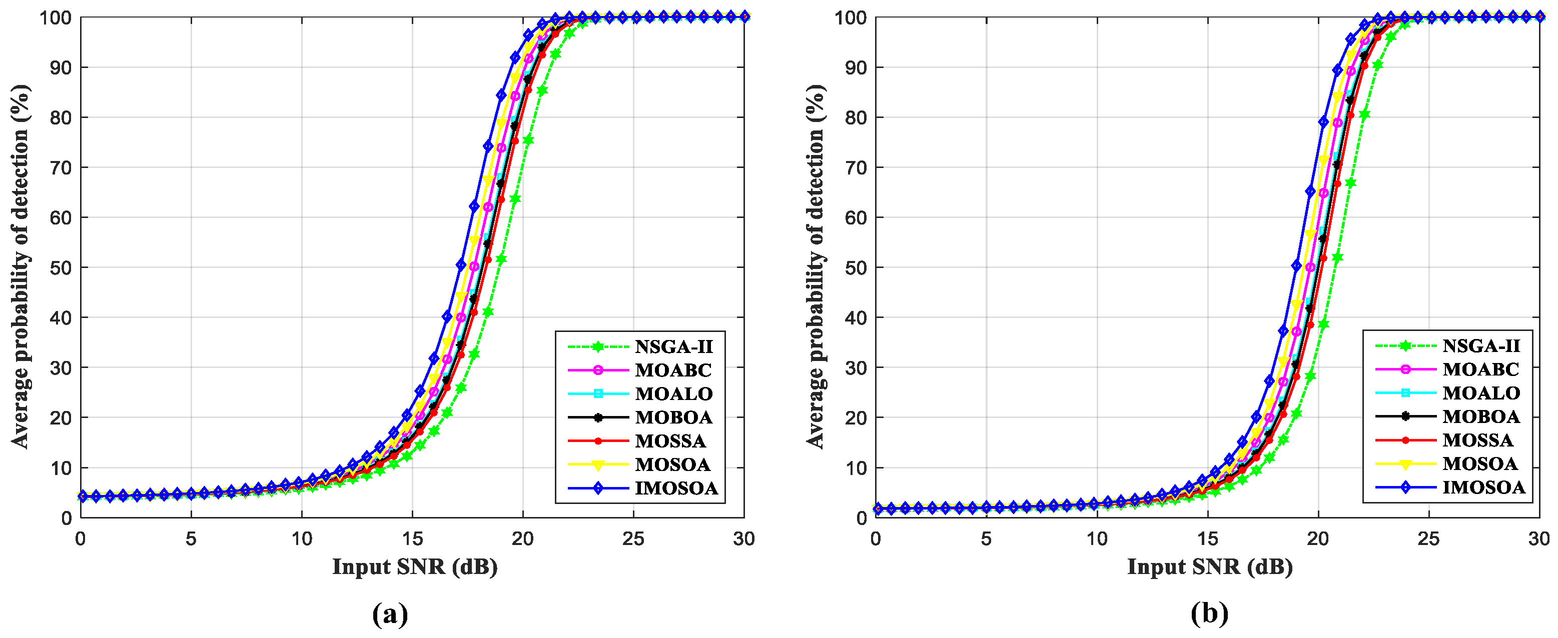
Optimization Algorithms	The Value of Objective Functions			Moving Target Detection Probability (PD)
	${\mathit{f}}_{\mathit{P}\mathit{U}\mathit{I}}$	${\mathit{f}}_{\mathit{S}\mathit{T}\mathit{D}}$	${\mathit{f}}_{\mathit{A}\mathit{P}\mathit{L}}$	False Alarm 10−4	False Alarm 10−6
NSGA-II	0.095	1.256	9.598	70.8%	34.6%
MOABC	0.100	1.184	8.514	88.8%	59.1%
MOSSA	0.098	1.130	8.724	81.4%	46.6%
MOALO	0.096	1.042	8.814	84.9%	51.8%
MOBOA	0.096	1.065	8.936	83.9%	50.2%
MOSOA	0.097	1.015	8.225	91.8%	65.8%
IMOSOA	0.096	1.005	7.914	94.6%	73.7%

. We can see that the values of PUI show almost no difference between the comparison methods, because the difference in the total length of the array aperture is less than 0.1 m. Compared with the values of APL and STD, we can conclude that the IMOSOA algorithm has significant advantages for improving the clutter suppression ability. Moreover, for the moving target detection probability in the case of input SNR = 20 dB, we can see that the detection performance of the radar system is improved about 25% by the proposed MOSOA and IMOSOA.

To further evaluate the quality of the optimal solution, an experiment was performed to obtain the system output SCNR-Loss curve of the final solution. In this experiment, the input signal-to-noise ratio of target was set to 25 dB, and the threshold of MDV was determined by the detection probability of 0.5. We set moving targets with the radial velocity uniformly changing in the interval [−40, 40] m/s. The SCNR-Loss of clutter suppression was calculated using the GMTI performance model in (8) and the CCM model in (10). Eventually, we obtained the output SCNR-Loss curve of each optimization algorithm, as shown in Figure 7.

From Figure 7, we can see that the undetectable interval (or the filter response “notch”) of the comparison methods show little difference. But the performance of the detectable interval of the proposed IMOBOA method is much better than that of the other methods. As shown in the right figure of Figure 7, the average processing loss and the fluctuations of the SCNR-Loss curve are much smaller than those of the other contrast methods. This indicates the better GMTI performance of the proposed IMOBOA method. This conclusion can be also demonstrated from Table 5, that is, the average processing loss $f_{APL}$ and standard deviation value of SCNR-Loss $f_{STD}$ in the detectable interval are the smallest. This result indicates that the GMTI performance, in terms of clutter suppression capability and blind speed, is significantly improved by the proposed IMOSOA method.

To further evaluate the GMTI performance of the optimal solution, we studied the detection performance of the proposed IMOBOA method. We simulated a moving target detection performance curve (PD versus SNR) under the Gaussian homogenous clutter background. Under the assumption of a non-fluctuating target, the velocity of moving targets uniformly distributed in interval [10 m/s, 40 m/s] and target input SNR changed in interval [0 dB, 30 dB]. Through Monte Carlo experiments, we obtained the average probability of detection (PD). Then, we obtained the detection performance curves of PD changing with input SNR, as shown in Figure 8. It is obvious that the proposed IMOBOA method outperformed the comparison methods in terms of moving target detection performance. Especially for the lower SNR target, the improvement in detection performance was more significant. The average detection probability of IMOSOA improved 30% (equivalently, the detection SNR improved 2 dB) compared with that of the NSGA-II method in the SNR interval [15 dB, 20 dB].

In summary, the clutter suppression capability, system MDV, and moving target detection performance indicators demonstrated that the GMTI performance of distributed array radar can be greatly improved by the proposed IMOSOA.

4.3. Performance of IMOSOA

This subsection performed two experiments to evaluate the solution quality and efficiency of the IMOSOA algorithm. There are two indicators that can be used as the criterions. (i) The solution quality can be evaluated by the uniformity of the Pareto front and the distance between the solution to the coordinate origin in the Pareto front. (ii) The efficiency of IMOSOA can be evaluated by the convergence speed. The experimental results were compared against those of NSGA-II, MOABC, MOALO, MOBOA, and MOSSA. Next, the simulation experiment results will be further investigated and discussed.

4.3.1. Solution Quality Evaluation

The first experiment mainly evaluated solution quality through comparing the Pareto front of different algorithms. In this paper, the smaller the values of the object functions, the better the GMTI performance. That is to say, the global optimal solution should approach the coordinate origin in the Pareto front. Therefore, we give the Pareto front obtained by different multi-objective optimization algorithms after iterative processing. Figure 9 depicts the Pareto front, wherein each point represents a solution at the Pareto front. The three axes represent the corresponding objective functions (the percentage of the undetectable interval $f_{PUI}$, the average processing loss $f_{APL}$, and the standard deviation $f_{STD}$ of the detectable interval).

Figure 9a depicts the Pareto front of the NSAG-II algorithm. It has good global convergence, but the phenomenon of local aggregation occurs, resulting in poor uniformity of the solution. Figure 9b depicts the Pareto front of the MOABC algorithm. It can be seen that the uniformity of the solution is very good. But its global convergence is poor because the points in the solution set are relatively scattered and far from the origin. Figure 9c depicts the Pareto front of the MOSSA algorithm where the points in the solution set converge into two parts in space. This indicates that partial solutions fall into a local optimum. Figure 9d depicts the Pareto front of the MOALO algorithm. The points in the solution space are far from the origin, so clearly, this solution is not the desirable outcome. Figure 9e depicts the Pareto front of the MOBOA algorithm. Its local convergence effect is good, but the solution is unevenly distributed in space. Figure 9f depicts the Pareto front of the MOSOA algorithm. We can see that the solutions in the front are clustered closer to the coordinate origin. Figure 9g shows the Pareto front of the proposed IMOSOA algorithm. It is obvious that each solution in its Pareto front is converged to a very small neighborhood of the origin, which indicates the superior global convergence performance of the algorithm. We can conclude that the solution quality of the proposed IMOSOA algorithm is much better than that of the comparison methods.

4.3.2. Convergence Speed Comparison

The convergence speed is a key point that most optimizations algorithm pay attention to. As described in Section 3, the main purpose of IMOSOA is to improve the convergence and effectiveness of MOSOA. Thus, the second experiment mainly compared the speed of convergence of each optimization algorithm.

For the multi-objective optimization algorithm, it is difficult to know the convergence time from multiple objective function values directly. But when the Pareto front is no longer updated, the number of solutions in the external file will remain unchanged. Therefore, convergence can be determined when the number of solutions in the Pareto front no longer changes. Figure 10 shows the variation in the number of solutions in the Pareto front of different optimization algorithms versus iteration times. From Figure 10, it can be seen that the MOBOA algorithm has the fastest speed of convergence, followed by the MOABC algorithm, then the IMOSOA and NSGA-II algorithms, and the MOSSA algorithm is the slowest.

In the above experiment, we could obtain the convergence speed (measured by iteration times) of each multi-objective optimization algorithm, as listed in

Table 6. The convergence speed of different methods.

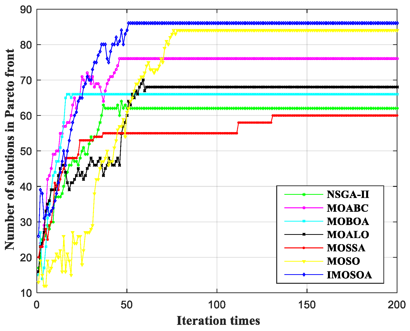
Optimization Algorithms	Iteration Number	Solutions Number
NSGA-II	51	62
MOABC	46	76
MOSSA	131	60
MOALO	61	68
MOBOA	20	66
MOSO	79	84
IMOSOA	51	86

. As can be seen, the convergence speed of the MOBOA algorithm is about 20 times; the convergence speed of the MOSO algorithm is 79 times; and the convergence speed of the IMOSOA algorithm is about 51 times. The improvement in convergence speed of our proposed method is very significant compared to that of the MOSOA algorithm. It is noteworthy that the number of solutions in the Pareto front of the proposed IMOSOA is larger than that of the other algorithms. This will enable the algorithm to preserve the diversity of the solution space and maintain its robustness. In conclusion, although the convergence speed of IMOSOA is a bit behind compared to that of the MOBOA algorithm, the improvement in solution quality is very significant.

4.4. Discussion of the Improvement of IMOSOA

The comparison results in Figure 10 and Table 6 show that the convergence speed of MOSOA is much slower than that of the other five typical multi-objective optimization algorithms. To address this issue, we proposed an improved MOSOA algorithm. We introduced tent chaotic mapping to generate initial solutions. The multi-group cooperative strategy was integrated into the evolutionary process to increase population diversity, thus improving convergence speed. Furthermore, we proposed the scale variable individual mutation strategy to reduce the risk of falling into a local optimum.

The experimental results proved that the IMOSOA algorithm has significant advantages compared with the original MOSOA algorithm. The improvement was demonstrated in the following three aspects. First, GMTI performance was enhanced greatly in terms of the clutter suppression capability and moving target detection performance indicators, as shown in Figure 7 and Figure 8. Second, the solution quality of the proposed IMOSOA algorithm is much better than that of MOSOA. Comparing Figure 9f,g, we can see that the solution distribution in the Pareto front of IMOSOA is more concentrated than that of MOSOA. Third, the convergence performance of IMOSOA has obvious advantages over that of MOSOA, as illustrated in Figure 10.

In summary, the proposed IMOSOA can achieve comprehensive improvement. This conclusion can be drawn from the perspective of the global convergence performance of the solutions at the Pareto front, as well as the GMTI performance of the final solution. Therefore, the IMOSOA algorithm provides an effective way to optimize the configuration of distributed arrays. It can obtain the global optimal solution more quickly and robustly, as well as achieve better GMTI performance of the system.

5. Conclusions

In this paper, a multi-objective intelligent optimization framework, IMOSOA, is developed for the optimal design of a distributed array configuration for SAR-GMTI applications. IMOSOA mainly has four contributions: establishing a multi-objective optimization problem to express the functional relationship between array position and GMTI performance indicators; combining the Pareto optimization mechanism to accomplish a tradeoff among conflicts between each objective and achieve optimal overall performance; and modifying the initialization process and evolution strategy of the SO algorithm to solve the global searching problem. The proposed IMOSOA takes the non-ideal factors of the real environment as objective functions, ensuring that it is suitable for real-world engineering applications. The solution quality and efficiency of IMOSOA are significantly improved through tent chaotic mapping, multi-group coevolution, and individual mutation strategies. To evaluate the effectiveness of the proposed method, numerical simulation experiments are compared against other five state-of-the-art algorithms. The experiments investigated the GMTI performance indicators of clutter suppression capability, system MDV, and moving target PD, as well as the convergence performance of solution quality and convergence speed. All of the indicators demonstrated that IMOBOA outperformed the comparison methods, and it has superior performance for the optimal design of radar array configurations. Precisely speaking, this work provides a simple yet effective approach to design radar arrays for system engineers.

In addition, this paper provides an application example for airborne distributed array SAR-GMTI systems (as well as spaceborne distributed array radar systems). IMOBOA can also be used to solve combinatorial multi-objective optimization problems, such as systematic decision, data dimension reduction, classification, image reconstruction, etc.

References

- Yang, L.; Wang, T.; Bao, Z. Ground Moving Target Indication Using an InSAR System with a Hybrid Baseline. IEEE Trans. Geosci. Remote Sens. Lett. 2008, 5, 373–377. [Google Scholar] [CrossRef]
- Budillon, A.; Gierull, C.H.; Pascazio, V.; Schirinzi, G. Along-Track Interferometric SAR Systems for Ground-Moving Target Indication: Achievements, Potentials, and Outlook. IEEE Geosci. Remote Sens. Mag. 2020, 8, 46–63. [Google Scholar] [CrossRef]
- Wendleder, A.; Wessel, B.; Roth, A.; Breunig, M.; Martin, K.; Wagenbrenner, S. TanDEM-X water indication mask: Generation and first evaluation results. IEEE J. Sel. Top. Appl. Earth Observ. Remote Sens. 2013, 6, 171–179. [Google Scholar] [CrossRef]
- Baumgartner, S.V.; Krieger, G. Dual-Platform Large Along-Track Baseline GMTI. IEEE Trans. Geosci. Remote Sens. 2016, 54, 1554–1574. [Google Scholar] [CrossRef]
- Rocca, P.; Haupt, R.L.; Massa, A. Sidelobe Reduction Through Element Phase Control in Uniform Subarrayed Array Antennas. IEEE Antennas Wirel. Propag. Lett. 2009, 8, 437–440. [Google Scholar] [CrossRef]
- Li, X.; Yang, Z.; Tan, X.; Liao, G.; Shu, Y. A Novel Knowledge-aided Training Samples Selection Method for Terrain Clutter Suppression in Hybrid Baseline Radar Systems. IEEE Trans. Geosci. Remote Sens. 2022, 60, 1–16. [Google Scholar] [CrossRef]
- Li, X.; Yang, Z.; He, S.; Huang, P.; Liao, G.; Jiang, Y. Nonhomogeneous clutter suppression based on terrain elevation interferometric phase compensation in multi-satellite formation systems. Digit. Signal Process. 2022, 121, 103282. [Google Scholar] [CrossRef]
- Li, X.; Wu, X.; Yang, Z.; Liao, G. A Closed-Form Expression of STAP Performance for Distributed Aperture Coherence MIMO Radar. IEEE Geosci. Remote Sens. Lett. 2024, 21, 1–5. [Google Scholar] [CrossRef]
- Li, W.T.; Shi, X.W.; Hei, Y.Q.; Liu, S.F.; Zhu, J. A Hybrid Optimization Algorithm and Its Application for Conformal Array Pattern Synthesis. IEEE Trans. Antennas Propag. 2010, 58, 3401–3406. [Google Scholar] [CrossRef]
- Yang, K. Optimisation method on conformal array element positions for low sidelobe pattern synthesis. IET Microw. Antennas Propag. 2012, 6, 646–652. [Google Scholar] [CrossRef]
- Li, H.; Jiang, Y.; Ding, Y.; Tan, J.; Zhou, J. Low-Sidelobe Pattern Synthesis for Sparse Conformal Arrays Based on PSO-SOCP Optimization. IEEE Access 2018, 6, 77429–77439. [Google Scholar] [CrossRef]
- Isernia, T.; Pena, F.J.A.; Bucci, O.M.; D’Urso, M.; Gomez, J.; Rodriguez, J. A hybrid approach for the optimal synthesis of pencil beams through array antennas. IEEE Trans. Antennas Propag. 2004, 52, 2912–2918. [Google Scholar] [CrossRef]
- Jarske, P.; Saramaki, T.; Mitra, S.K.; Neuvo, Y. On properties and design of nonuniformly spaced linear arrays (antennas). IEEE Trans. Acoust. Speech Signal Process. 1988, 36, 372–380. [Google Scholar] [CrossRef]
- D’Urso, M.; Prisco, G.; Tumolo, R.M. Maximally sparse, steerable, and nonsuperdirective array antennas via convex optimizations. IEEE Trans. Antennas Propag. 2016, 64, 3840–3849. [Google Scholar] [CrossRef]
- Yang, F.; Yang, S.; Chen, Y.; Qu, S.; Hu, J. Synthesis of sparse antenna arrays subject to constraint on directivity via iterative convex optimization. IEEE Antennas Wirel. Propag. Lett. 2021, 20, 1498–1502. [Google Scholar] [CrossRef]
- Gong, Y.; Shaoqiu, X.; Zheng, Y.; Wang, B. Synthesis of multiplepattern planar arrays by the multitask Bayesian compressive sensing. IEEE Antennas Wirel. Propag. Lett. 2021, 20, 1587–1591. [Google Scholar] [CrossRef]
- Elbir, A.; Mishra, K. Joint antenna selection and hybrid beamformer design using unquantized and quantized deep learning network. IEEE Trans. Wirel. Commun. 2020, 19, 1677–1688. [Google Scholar] [CrossRef]
- Hamza, S.A.; Amin, M.G. Sparse Array Design for Optimum Beamforming Using Deep Learning. IEEE Trans. Aerosp. Electron. Syst. 2024, 60, 133–144. [Google Scholar] [CrossRef]
- Chen, K.; Yun, X.; He, Z.; Han, C. Synthesis of sparse planar arrays using modified real genetic algorithm. IEEE Trans. Antennas Propag. 2007, 55, 1067–1073. [Google Scholar] [CrossRef]
- Jiang, Y.; Zhang, S.; Guo, Q.; Li, M. Synthesis of uniformly excited concentric ring arrays using the improved integer GA. IEEE Antennas Wirel. Propag. Lett. 2016, 15, 1124–1127. [Google Scholar] [CrossRef]
- Rocca, P.; Manica, L.; Stringari, F.; Massa, A. Ant colony optimization for tree-searching based synthesis of monopulse array antenna. Electron. Lett. 2008, 44, 783–785. [Google Scholar] [CrossRef]
- Oliveri, G.; Poli, L. Optimal sub-arraying of compromise planar arrays through an innovative ACO-weighted procedure. Prog. Electromag. Res. 2010, 109, 279–299. [Google Scholar] [CrossRef]
- Nouiri, M.; Bekrar, A.; Jemai, A.; Niar, S.; Ammari, A.C. An effective and distributed particle swarm optimization algorithm for flexible job-shop scheduling problem. J. Intell. Manuf. 2015, 29, 603–615. [Google Scholar] [CrossRef]
- Zhou, R.; Sun, J.; Wei, S.; Wang, J. Synthesis of conformal array antenna for hypersonic platform SAR using modified particle swarm optimization. IET Radar Sonar Navig. 2017, 11, 1235–1242. [Google Scholar] [CrossRef]
- Chhikara, R.R.; Sharma, P.; Singh, L. An improved dynamic discrete firefly algorithm for blind image steganalysis. Int. J. Mach. Learn. Cyber. 2016, 9, 821–835. [Google Scholar] [CrossRef]
- Smith, J.S.; Baginski, M.E. Thin-Wire Antenna Design Using a Novel Branching Scheme and Genetic Algorithm Optimization. IEEE Trans. Antennas Propag. 2019, 67, 2934–2941. [Google Scholar] [CrossRef]
- Li, Y.; Luo, J. Multi-objective self-organizing optimization for constrained sparse array synthesis. Swarm Evol. Comput. 2020, 58, 100743. [Google Scholar] [CrossRef]
- Cheng, Y.-F.; Shao, W.; Zhang, S.-J.; Li, Y.-P. An Improved Multi-Objective Genetic Algorithm for Large Planar Array Thinning. IEEE Trans. Magn. 2016, 52, 1–4. [Google Scholar] [CrossRef]
- Cao, A.; Li, H.; Ma, S.; Jing, T.; Zhou, J. Sparse circular array pattern optimization based on MOPSO and convex optimization. In Proceedings of the 2015 Asia-Pacific Microwave Conference (APMC), Nanjing, China, 6–9 December 2015; pp. 1–3. [Google Scholar]
- Ishibuchi, H.; Masuda, H.; Nojima, Y. Pareto fronts of many objective degenerate test problems. IEEE Trans. Evolut. Comput. 2016, 20, 807–813. [Google Scholar] [CrossRef]
- Ngatchou, P.; Zarei, A.; El-Sharkawi, A. Pareto Multi-objective Optimization. In Modern Heuristic Optimization Techniques; Lee, K.Y., El-Sharkawi, M.A., Eds.; John Wiley & Sons, Inc.: Hoboken, NJ, USA, 2008; pp. 189–207. [Google Scholar] [CrossRef]
- Deb, K.; Pratap, A.; Agarwal, S.; Meyarivan, T. A fast and elitist multiobjective genetic algorithm: NSGA-II. IEEE Trans. Evolut. Comput. 2002, 6, 182–197. [Google Scholar] [CrossRef]
- Erkoc, M.E.; Karaboga, N. A Novel Sparse Reconstruction Method based on Multi-objective Artificial Bee Colony Algorithm. Signal Process. 2021, 189, 108283. [Google Scholar] [CrossRef]
- Mirjalili, S.; Jangir, P.; Saremi, S. Multi-objective ant lion optimizer: A multi-objective optimization algorithm for solving engineering problems. Appl. Intell. 2016, 46, 79–95. [Google Scholar] [CrossRef]
- Rodrigues, D.; Albuquerque, V.H.C.D.; Papa, J.P. A Multi-Objective Artificial Butterfly Optimization Approach for Feature Selection. Appl. Soft Comput. 2020, 94, 106442. [Google Scholar] [CrossRef]
- Cheng, Z.; Wang, J. A new combined model based on multi-objective salp swarm optimization for wind speed forecasting. Appl. Soft Comput. 2020, 92, 106294. [Google Scholar] [CrossRef]
- Brennan, L.E.; Reed, L.S. Theory of Adaptive Radar. IEEE Trans. Aerosp. Electron. Syst. 1973, AES-9, 237–252. [Google Scholar] [CrossRef]
- Ender, J.H.G. Space-time processing for multichannel synthetic aperture radar. Electron. Commun. Eng. J. 1999, 11, 29–38. [Google Scholar] [CrossRef]
- Cerutti-Maori, D.; Sikaneta, I.; Gierull, C.H. Optimum SAR/GMTI Processing and Its Application to the Radar Satellite RADARSAT-2 for Traffic Monitoring. IEEE Trans. Geosci. Remote Sens. 2012, 50, 3868–3881. [Google Scholar] [CrossRef]
- Tang, B.; Tang, J.; Peng, Y. Detection of heterogeneous samples based on loaded generalized inner product method. Digit. Signal Process. 2012, 22, 605–613. [Google Scholar] [CrossRef]
- Xu, H.; Yang, Z.; He, S.; Tian, M.; Liao, G.; Sun, Y. A generalized sample weighting method in heterogeneous environment for space-time adaptive processing. Digit. Signal Process. 2018, 72, 147–159. [Google Scholar] [CrossRef]
- Melvin, W.L.; Showman, G.A. An approach to knowledge-aided covariance estimation. IEEE Trans. Aerosp. Electron. Syst. 2006, 42, 1021–1042. [Google Scholar] [CrossRef]
- Yang, Z.C.; de Lamare, R.C. Enhanced knowledge-aided space-time adaptive processing exploiting inaccurate prior knowledge of the array manifold. Digit. Signal Process 2016, 60, 262–276. [Google Scholar] [CrossRef]
- Li, Z.; Liu, H.; Zhang, Y.; Guo, Y. Robust nonhomogeneous training samples detection method for space-time adaptive processing radar using sparse-recovery with knowledge-aided. J. Appl. Remote Sens. 2017, 11, 045013. [Google Scholar] [CrossRef]
- Bento, M.; Ramon, P.; Luis, C. Considerations About Forward Fuselage Aerodynamic Design of a Transport Aircraft. In Proceedings of the 42nd AIAA Aerospace Sciences Meeting and Exhibit, Reno, NV, USA, 5–8 January 2004. [Google Scholar]
- Gracheva, V.; Ender, J. Multichannel Analysis and Suppression of Sea Clutter for Airborne Microwave Radar Systems. IEEE Trans. Geosci. Remote Sens. 2016, 54, 2385–2399. [Google Scholar] [CrossRef]
- Ward, J. Space-Time Adaptive Processing for Airborne Radar; MIT Lincoln Lab: Lexington, MA, USA, 1994. [Google Scholar]
- Wang, H.; Fang, D.G.; Chow, Y.L. Grating lobe reduction in a phased array of limited scanning. IEEE Trans. Antennas Propag. 2008, 56, 1581–1586. [Google Scholar] [CrossRef]
- Gonzalez, J.H.; Bachmann, M.; Krieger, G.; Fiedler, H. Development of the TanDEM-X Calibration Concept: Analysis of Systematic Errors. IEEE Trans. Geosci. Remote Sens. 2010, 48, 716–726. [Google Scholar] [CrossRef]
- Huang, P.; Xia, X.; Liu, X.; Jiang, X.; Chen, J.; Liu, Y. A Novel Baseline Estimation Method for Multichannel HRSW SAR System. IEEE Trans. Geosci. Remote Sens. Lett. 2019, 16, 1829–1833. [Google Scholar] [CrossRef]
- Guerci, J.R. Theory and application of covariance matrix tapers for robust adaptive beamforming. IEEE Trans. Signal Process. 1999, 47, 977–985. [Google Scholar] [CrossRef]
- Chen, C.W. A Spectral Model for Multilook InSAR Phase Noise Due to Geometric Decorrelation. IEEE Trans. Geosci. Remote Sens. 2023, 61, 1–11. [Google Scholar] [CrossRef]
- Zebker, H.A.; Villasenor, J. Decorrelation in interferometric radar echoes. IEEE Trans. Geosci. Remote Sens. 1992, 30, 950–959. [Google Scholar] [CrossRef]
- Rizzoli, P.; Braeutigam, B.; Kraus, T.; Martone, M.; Krieger, G. Relative height error analysis of TanDEM-X elevation data. ISPRS J. Photogramm. Remote Sens. 2012, 73, 30–38. [Google Scholar] [CrossRef]
- Ke, L.; Zhang, Q.; Battiti, R. Hybridization of decomposition and local search for multiobjective optimization. IEEE Trans. Cybern. 2014, 44, 1808–1820. [Google Scholar]
- Li, Y.; Han, M.; Guo, Q. Modified Whale Optimization Algorithm Based on Tent Chaotic Mapping and Its Application in Structural Optimization. KSCE J. Civ. Eng. 2020, 24, 3703–3713. [Google Scholar] [CrossRef]
- Liu, F.; Liu, Y.; Han, F.; Ban, Y.-L.; Guo, Y.J. Synthesis of large unequally spaced planar arrays utilizing differential evolution with new encoding mechanism and Cauchy mutation. IEEE Trans. Antennas Propag. 2020, 68, 4406–4416. [Google Scholar] [CrossRef]
- Deb, K. Multi-objective optimisation using evolutionary algorithms: An introduction. In Multi-Objective Evolutionary Optimisation for Product Design and Manufacturing; Springer: London, UK, 2011; pp. 3–34. [Google Scholar]
- Knowles, J.; Corne, D. The Pareto archived evolution strategy: A new baseline algorithm for Pareto multiobjective optimisation. In Proceedings of the 1999 Congress on Evolutionary Computation (CEC99), Washington, DC, USA, 6–9 July 1999; Volume 1, pp. 98–105. [Google Scholar]
- Zhou, A.; Qu, B.-Y.; Li, H.; Zhao, S.-Z.; Suganthan, P.N.; Zhang, Q. Multiobjective evolutionary algorithms: A survey of the state of the art. Swarm Evol. Comput. 2011, 1, 32–49. [Google Scholar] [CrossRef]
- Dorigo, M.; Birattari, M.; Stutzle, T. Ant colony optimization. IEEE Comput. Intell. Mag. 2006, 1, 28–39. [Google Scholar] [CrossRef]
- Karaboga, D.; Basturk, B. A powerful and efficient algorithm for numerical function optimization: Artificial bee colony (ABC) algorithm. J. Global Optim. 2007, 39, 459–471. [Google Scholar] [CrossRef]
- Yang, X.-S. Firefly algorithm, stochastic test functions and design optimization. Int. J. Bio-Inspired Comput. 2010, 2, 78–84. [Google Scholar] [CrossRef]
- Mirjalili, S.; Lewis, A. The whale optimization algorithm. Adv. Eng. Softw. 2016, 95, 51–67. [Google Scholar] [CrossRef]
- Mirjalili, S.; Gandomi, A.H.; Mirjalili, S.Z.; Saremi, S.; Faris, H.; Mirjalili, S.M. Salp swarm algorithm: A bio-inspired optimizer for engineering design problems. Adv. Eng. Softw. 2017, 114, 163–191. [Google Scholar] [CrossRef]
- Assiri, A.S.; Hussien, A.G.; Amin, M. Ant lion optimization: Variants, hybrids, and applications. IEEE Access 2020, 8, 77746–77764. [Google Scholar] [CrossRef]
- Hussien, A.G.; Amin, M. A self-adaptive harris hawks optimization algorithm with opposition-based learning and chaotic local search strategy for global optimization and feature selection. Int. J. Mach. Learn. Cybern. 2021, 13, 309–336. [Google Scholar] [CrossRef]
- Hussien, A.G.; Heidari, A.A.; Ye, X.; Liang, G.; Chen, H.; Pan, Z. Boosting whale optimization with evolution strategy and gaussian random walks: An image segmentation method. Eng. Comput. 2022, 39, 1935–1979. [Google Scholar] [CrossRef]
- Hashim, F.A.; Hussien, A.G. Snake Optimizer: A novel meta-heuristic optimization algorithm. Knowl. Based Syst. 2022, 242, 108320. [Google Scholar] [CrossRef]