1. Introduction
Masonry bridges represent invaluable cultural heritage assets, bearing historical and architectural significance [
1]. Despite their importance, these structures confront numerous challenges jeopardizing their preservation and structural integrity. Factors such as aging, weathering, and inadequate maintenance practices contribute to their deterioration, exacerbated by erosion, scour, and river turbulence, especially during high water flows. Material degradation and color changes further exacerbate their decline. By comprehensively addressing challenges and exploring innovative approaches, this research seeks to sustainably preserve cultural heritage for future generations. Current conservation efforts rely on traditional methods, constrained by budgetary limitations and expertise scarcity. Emerging technologies like non-destructive testing, advanced materials, and detailed geomantic data from Light Detection and Ranging (LIDAR) and Unmanned Aerial Vehicle (UAV) photogrammetry offer promise but face limited integration. These technologies provide comprehensive insights into both the hydrodynamic impacts on the bridge and the material properties and structural conditions, thereby enabling more effective conservation strategies. Initially used for military observation and tactical planning, UAV applications have expanded into commercial, scientific, recreational, agricultural, surveying, and mapping fields [
2,
3].
The geomatics data acquired by several platforms (ground, UAV, airborne, satellite) and interdisciplinary collaboration are crucial, underscoring the necessity for holistic conservation strategies tailored to the unique needs of masonry bridges in cultural heritage preservation. Masonry arch bridges represent one of the oldest forms of bridge construction and continue to constitute a significant portion of bridge infrastructure in various nations. For instance, in the UK alone, there are approximately 40,000 such bridges, accounting for roughly 40% of the total stock. While these historic structures have historically demonstrated robust load-carrying capacity under vertical static and transient loads, factors such as deterioration, aging, weathering, increased traffic loads, and various man-made and natural hazards, including flash floods, have contributed to a notable incidence of damage or failures among masonry arch bridges across European countries [
4]. Bridges are vulnerable to failure due to factors such as scouring of foundation materials, overtopping, hydrodynamic forces, and debris accumulation [
5]. Hydraulic design and evaluations of bridges focus on flows that cause overtopping and scouring, and this section examines how future climate change may impact these conditions. Overtopping, particularly damaging to approach embankments, and hydrodynamic forces during submersion threaten bridge stability [
6]. Scouring of bed materials from bridge foundations is the most common cause of bridge failure [
7], with scour depth measured using the HEC-18 manual by FHWA. Bridge scour, caused by water erosion around piers or abutments, poses significant risks to structural integrity and public safety. Engineers must consider flow velocity, sediment transport, and erosion resistance in bridge design to mitigate these risks; proper scour assessment is essential as floods scouring bed material around foundations are a leading cause of bridge failures, threatening structural integrity and capacity [
8].
In recent years, climate change (CG) has posed diverse risks to infrastructure safety and performance, necessitating a thorough understanding of its potential impacts for effective adaptation and risk management. Despite some attention from researchers, this field remains largely unexplored [
9]. Bridges, for instance, face accelerated material degradation due to changing climate conditions. Higher temperatures, increased precipitation, and elevated carbon levels may exacerbate deterioration, leading to heightened flood risks. Sea level rise, driven by rising temperatures, intensifies flooding risks, impacting coral reefs that naturally shield coastlines [
10]. Additionally, climate-induced changes in ocean pH, temperature, and tropical cyclone patterns further endanger infrastructure. Increased scour rates, a common cause of bridge failure, are also exacerbated by climate change [
11]. Understanding these dynamics is critical for developing effective strategies to safeguard infrastructure against climate-related threats. Hydraulic failures often manifest abruptly, leading to substantial devastation.
With GC intensifying globally, such incidents are anticipated to persist. These failures primarily stem from scour, floods, and floe ices [
12]. Indeed, the inevitability of CG is marked by its broad effects: the warming of the atmosphere and oceans, precipitation, shifts, sea level rise, and increased greenhouse gases, all unparalleled in recent decades. This intertwines the natural and human domains, significantly impacting humanity. This impact is notably destructive, evident in the increased occurrence of extreme events such as floods, hurricanes, and heat waves [
13,
14]. The susceptibility of masonry vaulted arch bridges to floods varies depending on the circumstances. Enhanced assessment accuracy hinges on data pertaining to water velocity and debris mass specific to local conditions, necessitating on-site monitoring and potential extrapolation for longer return periods. CG exacerbates this issue, further emphasizing the need for comprehensive assessment strategies [
15]. During flood events, various forces exert pressure on masonry arch structures, including horizontal hydrostatic force, hydrodynamic drag and uplift forces, buoyancy (hydrostatic uplift) force when the arch or bridge deck is submerged, and potential impact forces from debris [
16]. Fluvial flooding poses risks of structural failure by introducing hydrostatic and hydrodynamic effects, alongside scour effects [
17]. Hydraulic processes are the primary cause of bridge failure and masonry arch bridges are especially vulnerable to scour-induced settlements. Therefore, early detection of anomalies related to scour is of utmost importance to the safe functioning of river bridges [
18].
Several software packages are available for modeling floods, each with its unique features and capabilities. For example, HEC-RAS (Hydrologic Engineering Center’s River Analysis System) is a widely spread software package developed by the U.S. Army Corps of Engineers for hydraulic modeling [
19,
20]. Indeed, Suriya et al. (2023) [
9] wrote about the scour of Musiri Bridge located in India using the Hydraulic Engineering Center’s River Analysis Simulation (HEC-RAS) software v6.5.0. Using HEC-RAS as the simulation software, Mo et al. (2023) [
21] investigated breach failures in earth-rock dams located along the Chengbi River. In the same way, Pucci et al. (2023) [
22] present a technique to derive fragility curves for single-span bridges considering hydrodynamic actions and driftwood, utilizing HEC-RAS software and Python scripts developed in-house.
Current hydrological models and software for flood analysis include various approaches, each with distinct advantages and limitations. HEC-RAS is widely used for hydraulic modeling, while HEC-HMS focuses on watershed precipitation–runoff processes, and SWMM is designed for urban runoff and storm water management. These models differ in scale, complexity, and computational needs. Hydrologic processes have applications in rainfall–runoff modeling, water supply–demand, streamflow computation, and extreme event analysis. Tamiru and Dinka (2021) [
23] integrated an ANN flood prediction technique with HEC-RAS to enhance flood prediction accuracy by generating time series runoff values used for flood inundation modeling. Sahu et al. (2023) [
24] reviewed state-of-the-art hydrological models, emphasizing the HEC-HMS model’s role in understanding and managing water resources, despite challenges like data acquisition and soil heterogeneity. Haliuc and Frantiuc (2012) [
25] analyzed flash floods in Romania’s Baranca drainage basin using HEC-RAS and HEC-GeoRAS v6.5.0. They validated simulations with data from 2010 flash floods, demonstrating the programs’ effectiveness in simulating water flow and floodway encroachments. The study highlighted the need for integrating these tools into flood management strategies to mitigate risks, despite ongoing construction in vulnerable areas. The field of hydraulic risk assessment and conservation of historic masonry bridges has advanced significantly with the integration of advanced technologies and comprehensive modeling techniques. Studies have employed HEC-RAS software for hydraulic modeling and risk assessment, analyzing various impacts on bridge stability.
Recent research includes Suriya et al.’s study (2023) [
9] on the Musiri Bridge in India, Mo et al.’s study (2023) [
21] on dam breaches along the Chengbi River, and D’Angelo et al.’s study (2022) [
26] on the Baghetto Bridge in Italy, all demonstrating the effectiveness of HEC-RAS in different contexts. Additionally, UAV photogrammetry and LIDAR data have revolutionized high-resolution topographical data collection. Açıl et al. (2021) [
27] used UAV data and HEC-RAS to determine the dimensions of hydraulic structures on forest roads, highlighting the model’s accuracy in evaluating drainage capabilities. Huţanu et al. (2020) [
28] demonstrated the use of 1D HEC-RAS and LiDAR data to improve flood hazard map accuracy, providing a realistic perspective on flood threats in the Jijia floodplain, Romania, compared to official maps. Ciurte (2023) [
29] successfully combined these technologies to study coastal erosion, achieving unprecedented accuracy.
However, there is still a gap in fully integrated methodologies that cover the entire process from data acquisition to hydraulic risk assessment, particularly for historic structures. Using 1D, 2D, and combined 1D/2D modeling techniques to identify flood-prone areas is crucial for flood hazard management projects, such as action plans for dam failure near large dams and reservoirs. The proposed work computes flood hazard models using the 2D HEC-RAS module, based on Digital Elevation Models (DEMs) derived from LiDAR data, and is pre- and post-processed using GIS-based software. Indeed, the present research uses the Saint-Venant equation to analyze river discharge and water depth. Key parameters include morphological data, hydrographs, rating curves, normal depth, and DEM. The focus is on hydraulic parameters’ relationship with flow characteristics, considering roughness coefficient variations, to help predict river behavior during floods. HEC-RAS software solves mass and momentum equations to calculate water surface profiles. It handles steady and unsteady flow, sediment transport, and water quality, generating flood maps with depth and velocity. HEC-RAS simulates various flow regimes for straight or dendritic rivers, requiring geometric data and boundary conditions. HEC-GeoRAS is used for geometric file preparation, assuming a constant energy head and perpendicular velocity vectors. Initial conditions include normal depth, discharge, and Manning’s “n” value. The model runs under unsteady conditions with defined upstream and downstream boundaries. HEC-GeoRAS defines initial and boundary conditions using GIS, providing input data for hydraulic parameters at cross-sections, including geometry, connectivity, and energy loss coefficients. The integration of UAV and LiDAR data with HEC-RAS for hydraulic modeling marks a significant advancement in the field. Therefore, this paper intends to illustrate a novel method to identify the risks by integrating UAV photogrammetry and LIDAR data into hydrodynamic models. This method differs from existing solutions by providing high-resolution topographical data and precise hydrodynamic simulations, thereby enhancing the accuracy of flood risk assessments for historical bridge structures. Historical architectural value is determined based on 3D reconstruction of the bridges and suitable hydraulic analysis using HEC-RAS software.
2. Method
To analyze the hydraulic risk assessment for the conservation of old masonry bridges, it is possible to identify the following main parts: (i) 3D geometry of the bridge; (ii) building a Digital Terrain Model (DTM) from airborne laser scanning (ALS) data for a length of about 100 m before and after the bridge; (iii) creating profiles along the river; (iv) hydraulic modeling utilizing Hydraulic Engineering Center’s River Analysis Simulation (HEC-RAS) 1D-2D Software; (v) scenario generation and analysis; and (vi) using HEC-RAS software v6.5.0. to analyze flow dynamics.
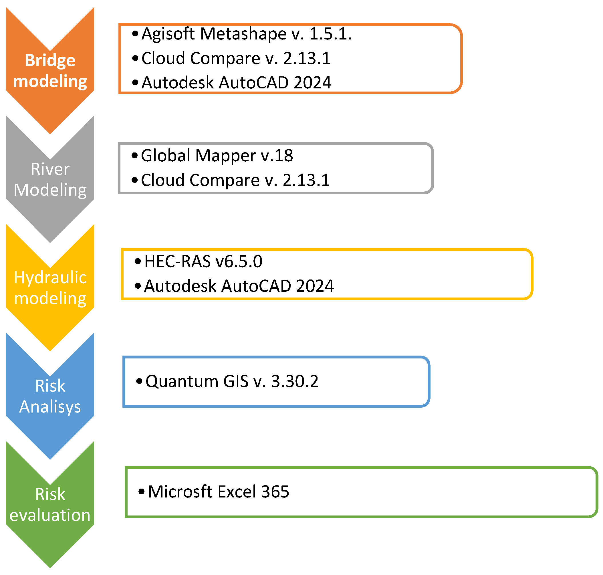
This study employs a multi-software approach to process and analyze data. The workflow includes the use of the following software:
- -
Cloud Compare (v2.13.1): This open-source tool is used for processing point clouds. It cleans the raw data from UAV photogrammetry and aerial LIDAR, removes noise and outliers, and merges point clouds from various sources to create a unified dataset.
- -
Autodesk AutoCAD (v2024): The processed point clouds are imported into AutoCAD for detailed vectorization. It enables the creation of accurate 2D and 3D drawings of bridge components, which are essential for hydrodynamic analysis.
- -
Quantum GIS- QGIS (v3.30.2): QGIS is used for geospatial analysis and visualization. It incorporates high-resolution orthophotos and digital terrain models (DTMs) from UAV and LIDAR data to analyze terrain features, riverbed morphology, and land use, aiding in hydrodynamic simulations.
The use of this latter software was related to the following tasks:
- -
Point Cloud Processing: Import, clean, and merge point cloud data with Cloud Compare, then export them for further use.
- -
Structural Modeling: Import the cleaned point clouds into AutoCAD to create detailed 2D and 3D models of the bridge, and export these models for hydrodynamic analysis.
- -
Geospatial Analysis: Use QGIS to import and analyze orthophotos and DTMs, visualize terrain and land use, and generate maps to support the hydrodynamic study.
The steps leading to bridge risk assessment can be carried out through the use of software, as shown in
Figure 1.
A key aspect of the vulnerability analysis of a masonry bridge concerns the 3D modeling, in particular Terrestrial Laser Scanning (TLS), UAVs, and terrestrial photogrammetry are techniques widely used in 3D geometry reconstruction of the structure. The data obtained from these techniques not only facilitate hydrodynamic simulations but also provide detailed information about the bridge’s material properties and structural conditions. This additional information can be crucial for assessing the bridge’s conservation needs and planning targeted restoration interventions. Especially in the photogrammetry context, thanks to developments in Computer Vision algorithms able to orientate a sequence of images in an easy and automatic way, such as Structure from Motion (SfM), the process of image orientation inherently involves creating a sparse 3D point cloud, which consists of tie points used for the relative orientation of images. These tie points are crucial for aligning the images. Multi-View Stereo (MVS) algorithms are used after the Structure from Motion (SfM) process to generate depth maps, dense point clouds, or 3D models. The MVS process is separate and results in a denser reconstruction compared to the sparse tie point cloud obtained during SfM [
30]. For example, Cavalagli et al. (2020) [
31] developed a procedure for a photogrammetric survey via UAV photogrammetry of masonry structures in order to obtain effective visual inspections and a 3D model of a historic masonry arch bridge located in Perugia (Italy). In the same way, Pepe et al. (2019) [
32] discussed the potential of a combined terrestrial and UAV photogrammetry approach in order to build a 3D model for Finite Element Method purposes. In this case study, UAV photogrammetry was tested in order to build the 3D model of the bridge.
The model can be inserted into a digital terrain model; naturally, the greater the detail of the terrain, the more reliable the quality of the hydraulic model. For example, the survey by ALS allows a very detailed point cloud to be obtained [
33]; in fact, by exploiting the possibility of obtaining information on the intensity of the signal, the number of rounds of the electromagnetic wave, and spatial information, it is possible to obtain a classification of the terrain. The classification of the terrain can be performed in several types of GIS software able to obtain the classified point cloud and, subsequently, build the DTM. HEC-RAS software (v6.5.0) from the U.S. Army Corps of Engineers’ Hydrologic Engineering Center is used to simulate the flow regime under the bridge. This hydraulic flow model identifies stream bank locations at each cross-section, dividing them into the left floodway, main channel, and right floodway. HEC-RAS uses input parameters such as river station number, lateral and elevation coordinates, bank station locations, reach lengths, Manning’s roughness coefficients, channel contraction and expansion coefficients, and geometric descriptions of hydraulic structures like bridges, culverts, and weirs [
34]. Ten scenarios were analyzed to evaluate the effect of the hydraulic flow regime on the bridge. The parameter considered was the flow discharge in the river channel, ranging from 2 m
3/s in the first scenario to 300 m
3/s in the tenth scenario.
Two-dimensional steady flow analysis is useful for calculating the water surface profile, assuming gradually varying flow along its length. It can determine the water surface profile for subcritical, supercritical, and mixed flow conditions. The governing equation for this calculation is the energy equation (Equation (1)) [
35]:
where Z
1 and Z
2 are the elevations of the bottom of the channel at cross-sections 1 and 2; Y
1 and Y
2 are the depths of water at cross-sections 1 and 2; V
1 and V
2 are the velocities of water at cross-sections 1 and 2; α
1 and α
2 are the velocity weighing factors; G is the acceleration due to gravity; and h
e is the energy head-loss.
Different flow rates should be included in the analysis to determine the level of drainage capacity to accommodate the flow rate as shown in the following equations (Equations (2) and (3)):
where Q is the ratio between the flow rate and discharge (evaluated in m
3/s), while V
n is the average velocity at cross-section n (m/s), and A
n is the area at cross-section n (m
2).
Q is the flow discharge, n is the Manning roughness coefficient; A is the flow area, R is the hydraulic radius, and Sf is the friction slope between two cross-sections.
To calculate the pressure exerted on a structure (bridge elements) by flowing water, we can use the principles of fluid dynamics, particularly Bernoulli’s equation. The dynamic pressure
Pdynamic is given by Equation (4):
where
ρ is the density of the water and
v is the velocity of the water.
3. Case Study
3.1. Identification of Study Area
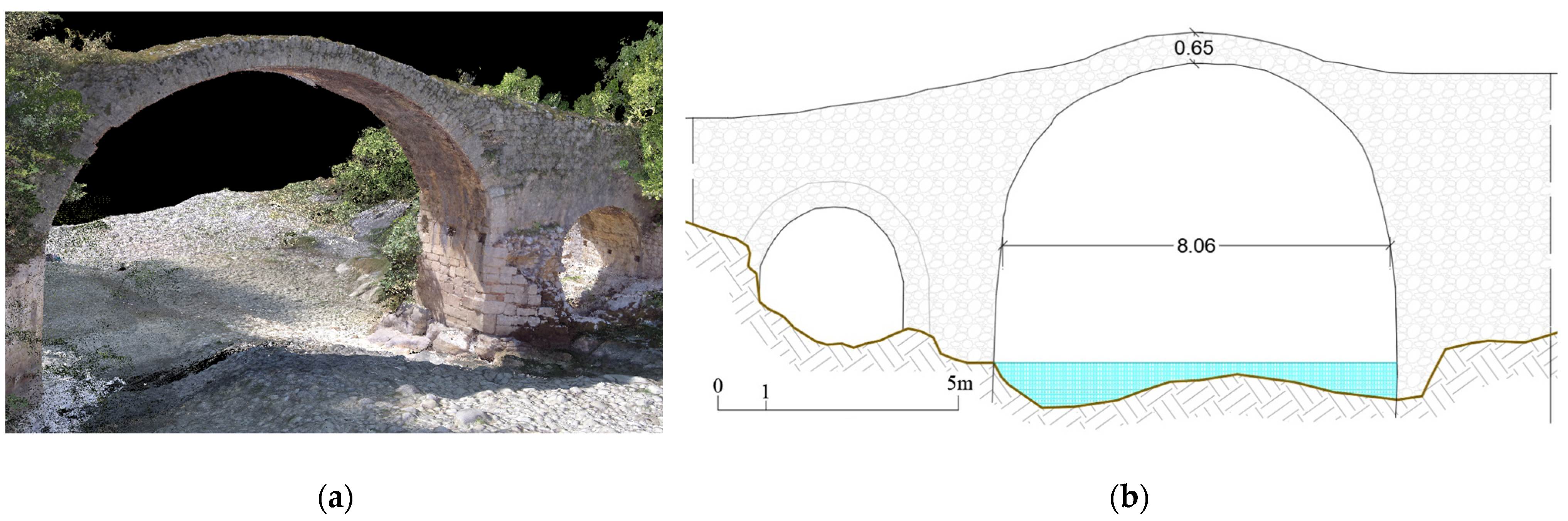
The research undertaken pertains to the examination of the Appian Way, focusing specifically on Hannibal’s Bridge, which is located on the border between the Campania and Basilicata regions, Italy (
Figure 2a), and is also known as Hannibal’s Bridge over the Melandro River (because of the belief that it was built by Hannibal on his way down south). In fact, that bridge crosses the Platano River, a tributary of the Melandro River, and is one of the oldest on Italic soil (
Figure 2b). Architecturally, the bridge is 3.45 m wide, 11 m high, and about 25 m long and is built with a single vault with two round arches, with large tuff boulders staggered to ensure greater stability, with respect to floods and possible earthquakes (
Figure 2c).
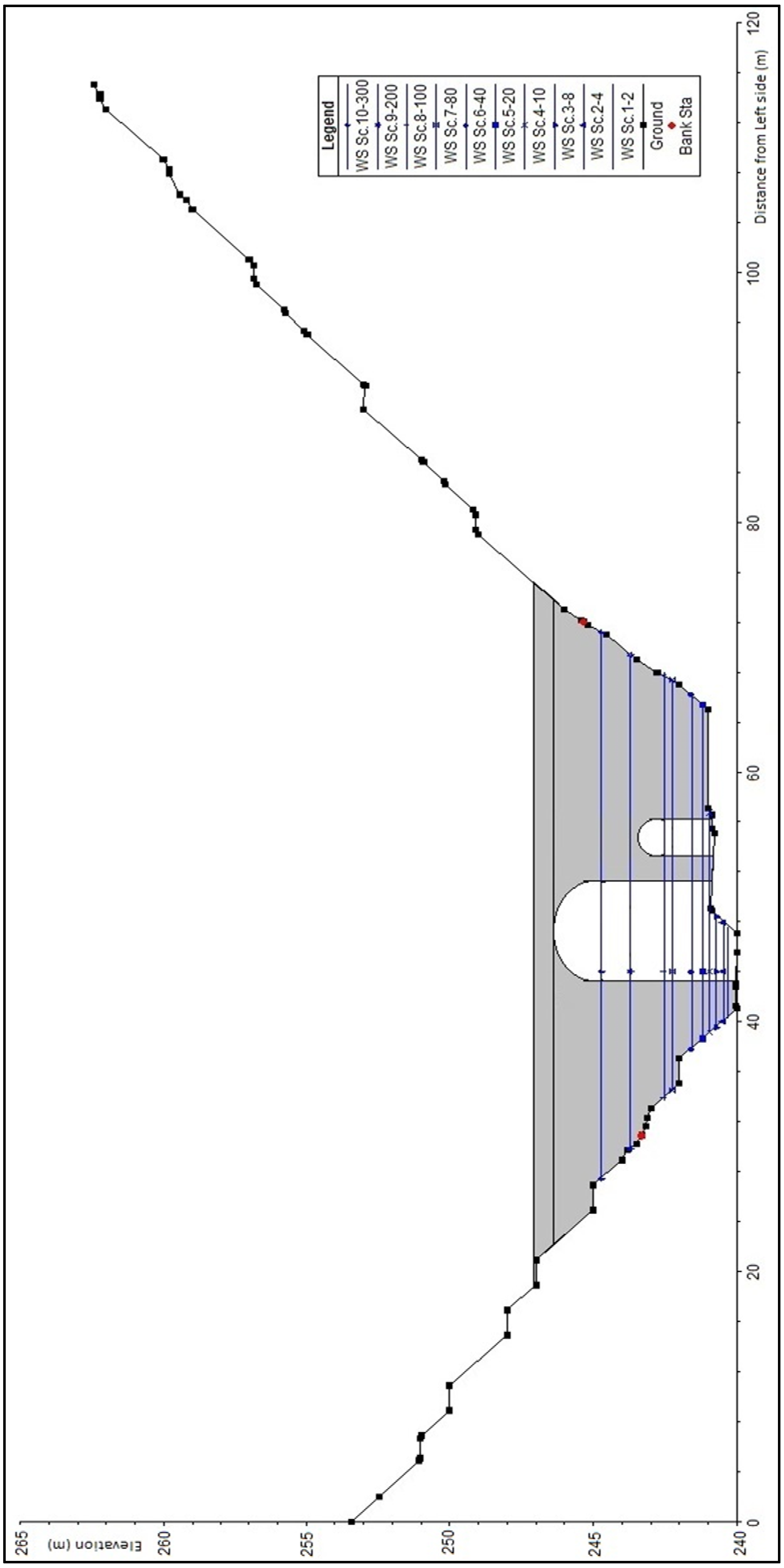
A hydraulic numerical model was developed utilizing HEC-RAS software to assess the water level dynamics along the course of the Platano River, particularly 400 m upstream of the bridge. This model aims to quantify the impact of varying water levels at this designated upstream location (Area A) on the bridge’s water level and structural integrity. The presence of the bridge, with its unique structural configuration including curves, narrow sections, and bottlenecks, is considered in the analysis to ensure that water levels remain within safe limits, avoiding overflow onto the adjacent banks. A DTM (Digital Terrain Model) map was obtained in the study area using Global Mapper software to build the hydraulic numerical model and find out the details of the terrain, topography, cross-sectional data, and highs and lows in the study area. The available points from the area map were interpolated so that the sectors could be drawn with an accuracy of 1 m. Twenty-three sections were used to build the hydraulic model in the case study area. The sections were created to be used as input data for the hydrological and hydraulic models.
Scenarios are generated to determine the maximum permissible (critical) water level upstream of the bridge, with provisions for monitoring and controlling water levels using staff meter gauges. In the event of water levels exceeding predetermined thresholds, precautionary measures such as the installation of vents, weirs, additional flow paths, and suction systems are recommended to mitigate potential risks associated with elevated water levels, pressure, and velocity on the bridge structure and its abutments.
This analysis focuses on identifying critical areas around the bridge, studying cross-sections and specific points of significance to understand flow patterns, vortices, dead zones, water velocity, and their implications on the bridge’s structural integrity.
Following scenario analysis, mitigation strategies are proposed to alleviate the severity of flow dynamics, vortices, erosion, and sedimentation. Modern hydraulic techniques, such as the strategic placement of small weirs upstream of the bridge and the implementation of specific venting mechanisms, are suggested to regulate water flow and minimize erosive forces, thereby safeguarding the structural integrity of the bridge and its surrounding infrastructure.
Furthermore, this study extends to assessing the impact of Platano River waters and rainfall on the bridge from both structural and architectural perspectives. This involves analyzing imagery obtained from field surveys to quantify the extent of vegetation growth, particularly green grass, on the bridge’s surface. By comparing the surface area coverage of vegetation to the original surface area of the bridge, insights into the structural implications of vegetation growth are gained, informing potential maintenance and preservation strategies.
3.2. Geomatics Data
The architectures of the bridge were obtained through UAV photogrammetry, which allowed the construction of a highly detailed 3D model. This model, combined with LIDAR data, not only supports hydrodynamic analysis but also provides extensive information about the materials and structural details of the bridge. By integrating these data into conservation models, we can better understand the degradation processes and develop more effective preservation strategies. Specifically, this model was obtained using 580 images acquired with Parrot Anafi UAV, equipped with a camera featuring a sensor size of 5344 × 4016 pixels, a pixel size of 0.0011 mm, and a focal length of 3.92 mm. Flight parameters included an average distance of 4 m from the bridge, resulting in a Ground Sample Distance (GSD) of about 0.1 cm/pixel.
Flight parameters included an average distance of 4 m from the bridge, resulting in a Ground Sample Distance (GSD) of about 0.1 cm/pixel; post-processing of the images was performed in Agisoft Metashape software, which enabled the generation of a point cloud of 23 million points (
Figure 3a). The final point cloud contained 23 million points, providing a high level of detail with a point density useful for 3D representation of the historical bridge, and it was essential to document the state of preservation to accurately model the bridge’s interaction with floodwaters. However, it was worth investigating whether reducing point cloud density would significantly impact hydrological analysis results. The processing settings in Agisoft Metashape were configured to balance detail and computational efficiency. To georeference the photogrammetric model, 7 Ground Control Points (GCPs) were used, evenly distributed around the bridge; in particular, 3 were placed on the arch of the bridge (extrados) while 4 others were placed along the riverbed, of which 2 were placed toward the south side and 2 toward the north side. The coordinates of the GCPs were obtained using GNSS Emlid Reach RS2+ instrumentation in Network-Real Time Kinematic mode [
36] and in the RDN2008 UTM Zone 33N reference system (EPSG: 7792). The spatial coordinate was transformed into orthometric elevation using the Italgeo05 model [
37] (a local geoid model with high accuracy) and, subsequently, to project the points into the WGS84/UTM zone 33N (EPSG: 32633) reference system. The accuracy of the alignment process was evaluated using the Total Error (TE), i.e., the root mean square error for x, y, and z coordinates; the TE achieved in this case study was 10 mm.
In addition, from the 3D mesh model, orthophotos were generated in order to create plans and façades of the masonry bridge; in fact, in the CAD environment, the façade of the bridge with the metric features of the bridge was built (
Figure 3b).
As for LIDAR data for the area around the river, a raw point cloud provided by the Italian Ministry of Environment was used. The point cloud has a density of 3/4 points per square meter. The precision on the point clouds is approximately 30 cm in planimetry and 15 cm in height. The point cloud is georeferenced in the WGS84 Reference System (EPSG 4326) with ellipsoid height. Therefore, before classifying the point cloud, it is necessary to transform the point cloud into orthometric elevation using the Italgeo05 model and, subsequently, to project the points into the WGS84/UTM zone 33N (EPSG: 32633) reference system. The classification process was carried out through the use of Global Mapper software [
38,
39], which offers robust, intuitive, and efficient tools for processing and classifying point cloud data. In such an environment, the classification process in Global Mapper can be performed in main steps: (i) import of point cloud data (LAZ file); (ii) initial filtering and preparation of data (noise reduction and terrain classification using suitable algorithms to identify and separate ground points from non-ground points); (iii) automatic classification of points into predefined categories such as terrain, vegetation (low, medium or high based on height thresholds), man-made structures and water surfaces, buildings, and other structures. With the ground points filtered, it is possible to build a gridded model in Global Mapper software, or better, to build the Digital Surface Model by going to the “Analysis” menu and selecting “Create Elevation Grid from 3D Vector Data”. In the dialog box, the “Create grid from LiDAR data” option was selected, and the grid spacing (1 m × 1 m) and the interpolation method (Triangulated Irregular Network -TIN) were set. In this way, it was possible to generate and subsequently export the DTM in the GEOTIFF format.
4. Results
The hydraulic model was run under ten different flow scenarios to evaluate the impact of varying discharge rates on water depth, water velocity, and dynamic pressure on the bridge using the Hydraulic Engineering Center’s River Analysis Simulation (HEC-RAS) software. Additionally, the integration of LIDAR and UAV photogrammetry data into these models allows for a more detailed analysis of the bridge’s material and structural conditions. This dual approach not only assesses the hydrodynamic risks but also supports the bridge’s conservation by identifying areas that require structural reinforcement or material restoration. The results are summarized in
Table 1 at the bridge upstream section.
As the discharge rate (Q) increases, the water depth also increases. This relationship is evident from the data, showing a progression from 0.31 m at 2 m3/s (Scenario 1) to 4.73 m at 300 m3/s (Scenario 10). The relationship between discharge and water depth indicates the ability of the channel to accommodate higher flows, though the increase in depth is not linear, reflecting the complex nature of river hydraulics and channel geometry. Water velocity also increases with discharge. Starting at 0.33 m/s for a flow of 2 m3/s, it rises to 9.79 m/s at 300 m3/s. Notably, the increase in velocity is relatively modest up to Scenario 8 (100 m3/s) but shows a significant jump in Scenarios 9 and 10, indicating possible changes in flow regime or channel characteristics that could lead to higher velocities at greater discharges. Dynamic pressure (P.dynamic) exhibits a similar trend, increasing with discharge. It rises from 55.03 Pa at 2 m3/s to 47,934.75 Pa at 300 m3/s. This significant increase is particularly pronounced at higher discharges, as indicated by the rapid escalation from Scenario 8 to Scenario 10. This dynamic pressure is a critical parameter for understanding the forces exerted by the flowing water on structures within the channel, such as bridge piers and abutments.
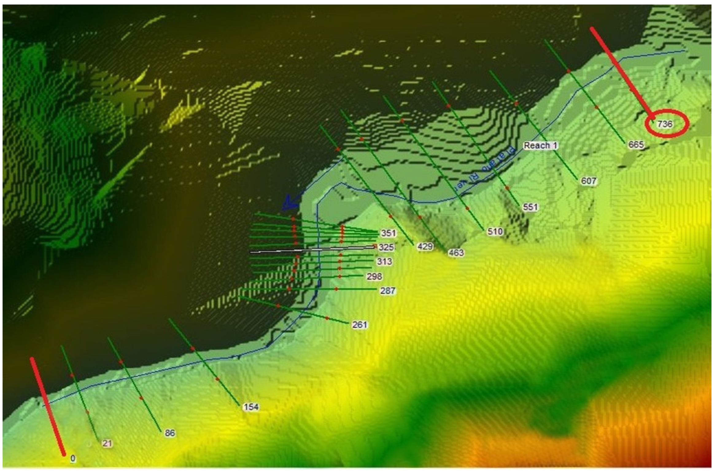
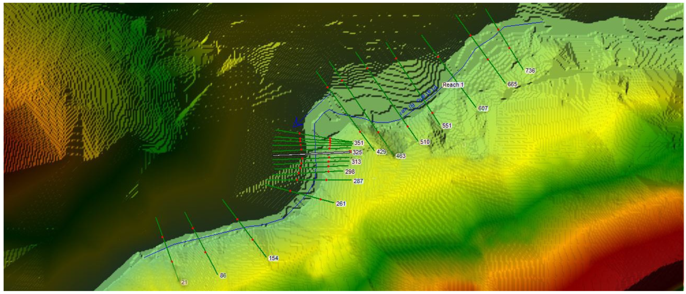
In the context of the HEC-RAS software, a “station” refers to a specific location along the river or stream where a cross-section is defined. Each cross-section is identified by a station number, which represents its position relative to a reference point, typically the downstream end of the river reach (in this study, 325 m after the bridge). These station numbers are used to organize and reference the various cross-sections within the model, facilitating the analysis and visualization of the river’s hydraulic properties at different points along its course.
Station 736 (cross-section 400 m before the bridge): This station is called 736 because it is the first cross-section station of the model in the upstream direction; the software numbers the stations from 0 at the suction or drained point or downstream of the model to the last station (the total length) of the study area model, and all sections between the first and last stations are numbered by the length from Station 0 as shown in
Figure 4.
This station exhibits a steady increase in water level with increasing discharge, indicating a predictable response to rising flow rates.
As shown in
Figure 5, the water level at Station 736 consistently rises as the discharge increases.
This pattern reflects the hydraulic behavior of the river upstream of the bridge, demonstrating that the river channel can efficiently convey the increasing volumes of water. This predictable response is crucial for understanding how the river will behave under various flow conditions and for designing effective flood management strategies. A meter gauge can be installed approximately 400 m upstream of the bridge to monitor the height of the water above the riverbed.
This reading should not exceed four meters to avoid posing a danger to the bridge. By knowing the water height at this gauge, the corresponding water discharge can be determined using
Table 2.
This approach allows for the real-time monitoring and assessment of hydraulic conditions, enabling timely interventions to prevent potential damage to the bridge.
Upstream of the bridge: this area shows a more gradual increase in water level compared to Station 736. This behavior is likely due to the upstream flow dynamics, which can moderate the rate of water level rise. The water levels here increase predictably but at a slower rate than those closer to the bridge, indicating that the upstream conditions play a significant role in influencing the flow characteristics.
Downstream of the bridge: The water level trends here are similar to those observed upstream of the bridge, but with slight variations. These variations suggest that local factors, such as the bridge structure or changes in channel morphology, impact how water levels respond to different discharge rates.
Station 0 (cross-section after the bridge by 325 m): This station exhibits the lowest water levels among all locations for the same discharge values. This can be attributed to its specific position in the watershed, where water may spread out or the channel may widen, leading to lower depths.
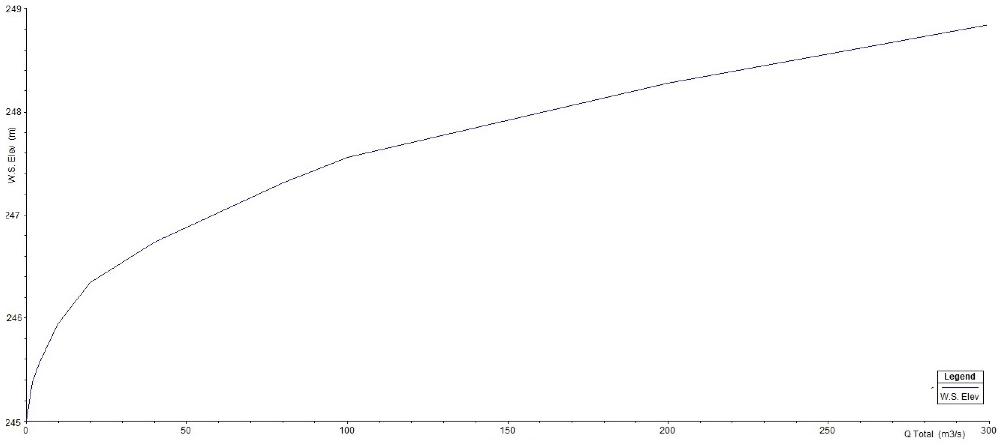
As illustrated in
Figure 6, where the X-axis represents the water discharge (m
3/s) and the Y-axis represents the water depth (m), Station 0 consistently shows reduced water depths compared to other measured points, reflecting the downstream dispersal of flow. The graph includes four distinct curves: Station 736 (blue curve), Upstream Bridge (red curve), Downstream Bridge (green curve), and Station 0 (purple curve). All curves exhibit an increasing trend, indicating that water surface level increases with an increase in discharge. The slopes of the curves are generally upward, consistent with typical rating curve behavior. Station 736 and Station 0: Both curves follow a similar pattern and remain close to each other throughout the range. This suggests that the hydraulic characteristics at these two stations are similar. Upstream Bridge: The curve for the Upstream Bridge is slightly above the Station 736 and Station 0 curves, indicating a higher discharge for the same stage. This could be due to structural or locational factors influencing the flow at the UP Bridge. Downstream Bridge: This curve is consistently below the others, indicating a lower discharge for the same water stage. This suggests that the Downstream Bridge (DN Bridge) has different hydraulic conditions, potentially due to flow constrictions, backwater effects, or other downstream conditions.
Curve behavior: At lower stages of discharge (0–50 cubic meters per second), the curves are relatively close, indicating minor differences in discharge across the locations and structures. As the stage increases beyond 50 cubic meters per second, the differences become more pronounced. The Downstream Bridge curve shows the least increase in discharge, while the Upstream Bridge curve shows the highest, with the Station 736 and Station 0 curves lying in between. At higher stages (200–300 cubic meters per second), the Upstream Bridge curve continues to show higher discharges compared to the other curves, suggesting that this bridge can handle higher flows more effectively. The Station 736 and Station 0 curves tend to converge at higher stages, indicating similar discharge capacities under extreme conditions. The differences in the rating curves imply varying hydraulic behaviors influenced by local conditions such as bridge design, channel geometry, and possible flow obstructions. Understanding these differences is crucial for accurate flood forecasting, hydraulic modeling, and designing mitigation measures. The lower discharge at Downstream Bridge highlights the need for potential interventions to manage lower flow capacities, which might include structural modifications or maintenance to improve flow efficiency.
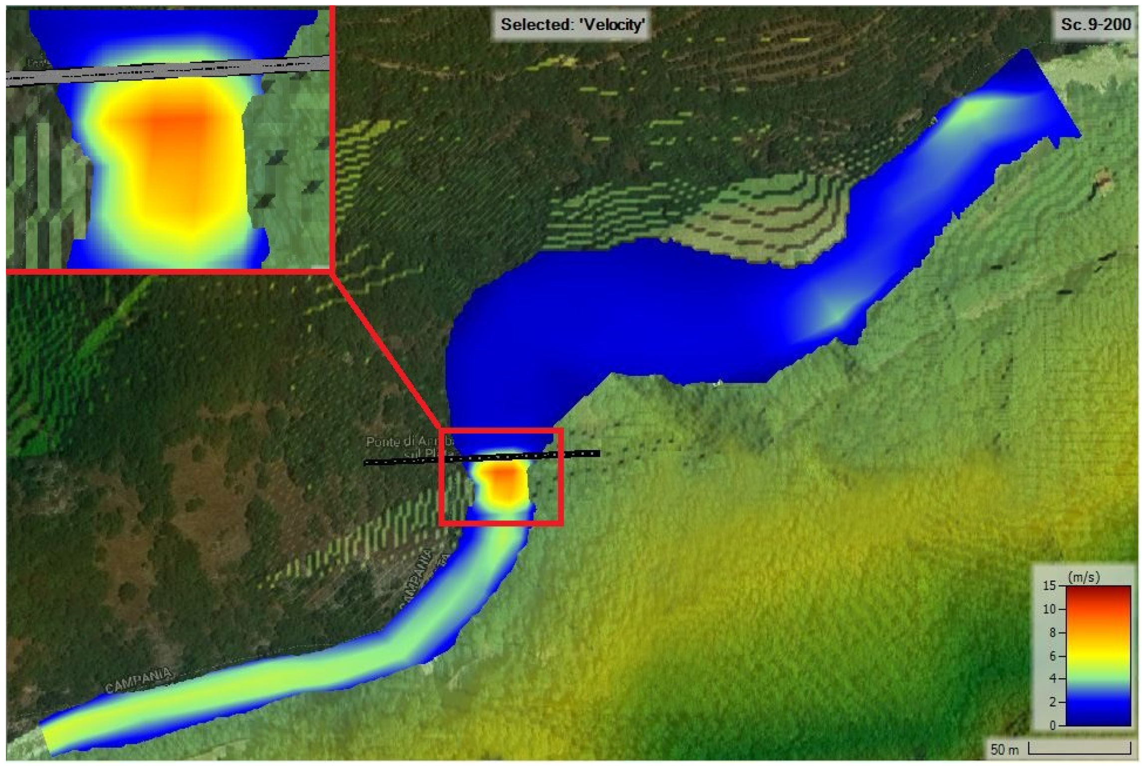
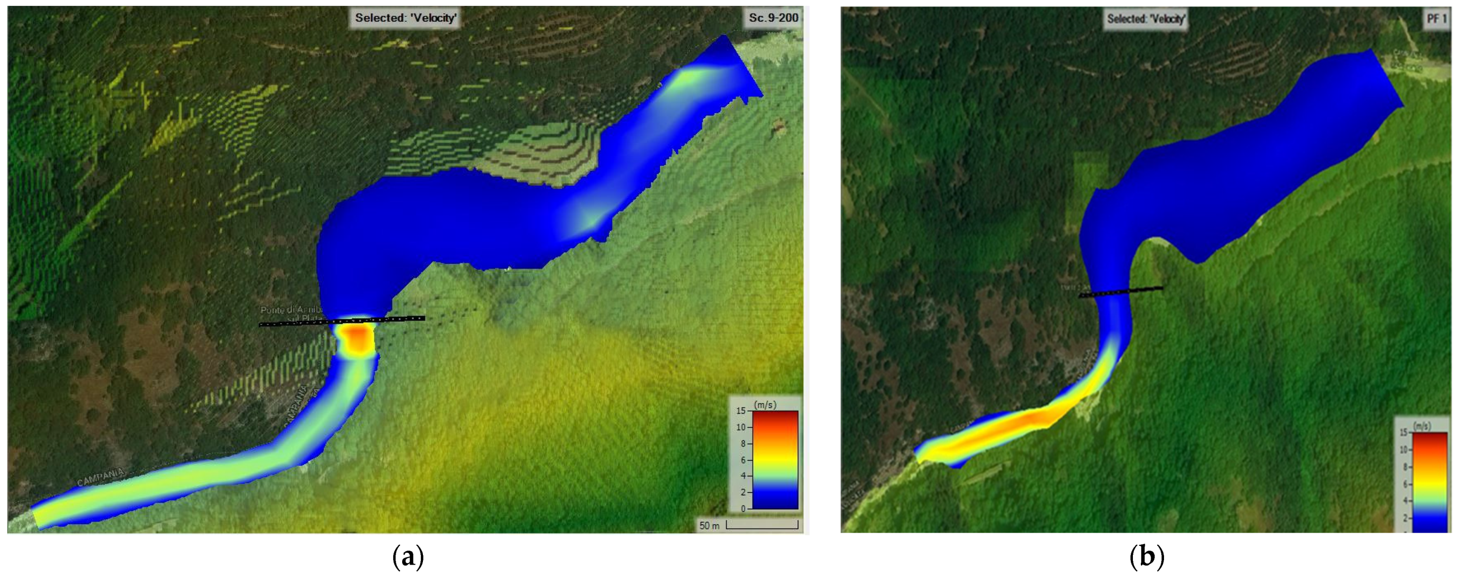
Figure 7 illustrates the velocity distribution of the river in the study area under a scenario with a water discharge of 300 m
3/s. The results indicate that water velocity is significantly higher around the bridge and downstream of the bridge. This increase in velocity can be attributed to the larger volume of water being funneled through the restricted openings of the bridge. The constriction causes an acceleration of flow as the water passes through and exits the bridge structure, resulting in higher velocities in these areas. Understanding this velocity distribution is crucial for assessing potential erosion risks and structural impacts on the bridge and adjacent areas.
In the study area, the most appropriate use of Manning’s coefficient is 0.03, and the longitudinal slope of the river is 9 m/km.
The maximum allowable water depth in front of the bridge is 4.73 m. Exceeding this depth will negatively affect the bridge and may lead to its collapse, as shown in
Appendix A.
5. Discussion
The method described has allowed us to create realistic scenarios on the hydraulic risk to which a structure is subjected. It is necessary to focus attention on two important aspects: climate change and the importance of the DTM.
5.1. Climate Change Impacts
Climate change impacts flow rates in rivers and streams through a complex interplay of increased precipitation, temperature-induced changes in snow and glacial melt, evapotranspiration dynamics, and human-induced land use changes. Understanding these interactions is crucial for predicting and managing future hydrological conditions and ensuring sustainable water resource management.
Climate change is expected to increase the frequency and intensity of heavy rainfall events, leading to higher peak flow rates in rivers and streams as more water enters the watershed in a shorter period. Changes in precipitation patterns, including shifts in the timing and distribution of rainfall, can alter flow regimes, with regions experiencing more intense rainy seasons seeing significant increases in flow rates during those periods. Rising temperatures can lead to earlier and more rapid snowmelt in mountainous regions, resulting in higher flow rates during spring and early summer as more water enters rivers over a short duration.
Additionally, higher temperatures can increase evaporation rates from water bodies and soil, potentially reducing base flow rates during dry periods, though this effect can be offset by increased precipitation in some regions. All these factors contribute to increased runoff, which collects from various tributaries and flows from higher elevations to lower ones, ultimately generating river discharge.
5.2. Impact of DEM in Hydraulic Modeling
The Shuttle Radar Topography Mission (SRTM) data, commonly used in Google Earth, and DTMs created using LiDAR data, often obtained through ALS, differ significantly in resolution and accuracy.
SRTM data provide a global resolution of 30 m (1 arc-second), suitable for regional- and national-level analyses but lacking the detail required for local or site-specific studies. In contrast, LiDAR data offer much higher resolution, typically between 0.5 and 2 m, with potential for even finer detail depending on scan density. This high resolution is ideal for detailed studies in urban planning, forestry, and precise topographic mapping. The vertical accuracy of SRTM data is generally around 10 m, varying with terrain and other factors, and their horizontal accuracy is typically within 10–20 m. Factors like vegetation and buildings can affect SRTM accuracy, introducing errors in elevation readings. LiDAR data, however, generally boast a vertical accuracy of 10–20 cm and a horizontal accuracy of 1 m or better, making it suitable for applications requiring precise elevation data, such as flood modeling, landslide analysis, and infrastructure development. SRTM data were collected using radar interferometry during an 11-day mission of the Space Shuttle Endeavour in 2000. The radar sensors captured elevation data using dual antennas to measure the phase difference and calculate surface elevations. LiDAR/ALS data, on the other hand, are collected using airborne sensors that emit laser pulses towards the ground, measuring the time taken for the pulses to return after reflecting off the surface. This method allows for the detection of multiple returns from different surface levels, enabling the creation of detailed models of both terrain and vegetation canopy.
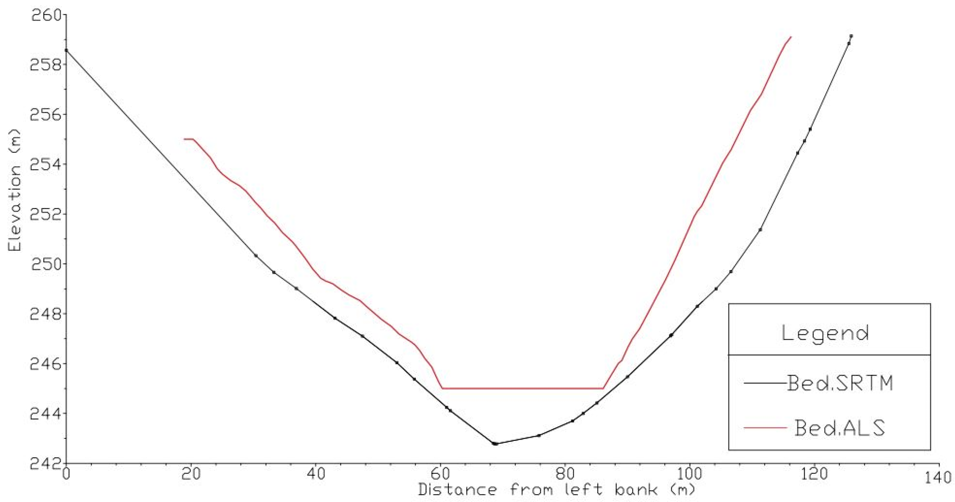
After running the hydraulic model using the two sets of geometric data, the results indicated that the bed level of the river channel upstream of the bridge (from Station 740 to Station 325) is approximately four meters lower in the SRTM geometry data compared to the ALS geometry data. Additionally, the interpolation of the elevation model in the SRTM data is poor, as evidenced by the cross-section at Station 736 (
Figure 8).
This discrepancy is also noticeable in the longitudinal profile, which affects the water surface elevation.
Figure 9 shows that the green line represents the water surface level obtained via the ALS method. The data indicate a horizontal profile before the bridge, signifying an unobstructed and regular flow within the channel. The longitudinal slope of the channel remains consistent until the water encounters the bridge, passes through its openings, and subsequently experiences a hydraulic jump. Post-bridge, the flow reverts to its regular characteristics. The red line illustrates the streambed level as determined by the ALS method, revealing a consistent longitudinal slope throughout the study area. Conversely, the blue line depicts the water surface level derived from the SRTM method. It demonstrates a horizontal profile before the bridge, followed by a marked drop after the bridge. Lastly, the black line represents the streambed level from the SRTM method, highlighting the presence of a small plateau after the bridge, which impacts the stream and alters the water flow.
The difference in water velocity at the bridge, influenced by these geometric variations, shows a 31.20% reduction in accuracy for the SRTM data. The difference between the ALS and SRTM methods is quantified by a mean difference of 3.53 and a standard deviation of 7.57. The impact of the choice of a specific DTM, or better, the impact of the difference in resolution and accuracy was significant, as shown in
Figure 10, as demonstrated by the cross-sections extracted from the geometric data and the longitudinal profile of the model. This difference also affected the distribution of water velocity. With the change in geometry, the cross-sections were altered, which subsequently modified the shape of the watercourse. This alteration affected the accuracy of the connections, leading to changes in the results.
Additionally, the difference in velocity distribution in the model is significant. The ALS data provide more accurate results, particularly at the bridge and after, where a large volume of water passes through a narrow opening. According to the equation
Q =
A⋅
v (where
Q is the constant discharge,
A is the cross-sectional area, and
v is the water velocity), the velocity must increase as the cross-sectional area decreases. In the bridge area, where the discharge remains constant along the river channel, the flow transitions from a larger cross-section to the narrower bridge opening, resulting in higher water velocity at and immediately after the bridge. This effect is accurately captured in the ALS model as shown in
Figure 11.
This study’s integration of UAV photogrammetry and LIDAR data into hydrodynamic models offers significant advancements over similar case studies. Compared to Hackl et al. (2018) [
40], who used UAV photogrammetry for topographical information, our approach includes a more detailed hydrodynamic simulation. Additionally, the work by Ccanccapa et al. (2024) [
41] focused on heritage riverine bridges with a hydrological approach but did not achieve the same level of integration of structural and hydrodynamic data. Our study contributes to the field by providing a comprehensive method that enhances both the accuracy of flood risk assessments and the potential for conservation strategies.
6. Conclusions
The integration of geomatics data and techniques in hydraulic risk assessment significantly enhances the conservation efforts for old masonry bridges, exemplified through the use of HEC-RAS modeling. By leveraging advanced geospatial data and techniques, geomatics provides precise and comprehensive information about topography, land use, and hydrological conditions. This data integration allows for accurate simulation and analysis of hydraulic behaviors under various flow conditions, aiding in the identification of potential risks and vulnerabilities in bridge structures.
Understanding the rating curves is essential for effective water resource management and flood forecasting. These curves provide a reliable method for estimating discharge based on observed water levels, aiding in the monitoring and management of the waterway. When the meter gauge reading at Station 736, located before the bridge, exceeds a value of 4, be aware that the water velocity at the bridge will exceed 9. This increased velocity can impact the bridge structure and cause scouring on the river channel bed and downstream bed of the bridge.
The HEC-RAS program used in this study gave accurate results in the hydraulic numerical model using geometry data (DTM) in the study area. HEC-RAS furnishes the flood profile for the most severe flood scenario, aiding in the selection of suitable measures for mitigating flood disasters. Utilizing HEC-RAS for flood modeling proves to be a powerful tool for hydraulic analysis and implementing disaster management strategies. The curves indicate that as discharge increases, water levels rise at all stations and bridges. The differences in water levels at the same discharge can be attributed to the specific hydraulic characteristics of each location.
The integration of geomatics in hydraulic risk assessment through HEC-RAS modeling significantly improves the conservation of masonry bridges by providing precise topographical and hydrological data for accurate simulations. Moreover, the detailed information obtained from LIDAR and UAV photogrammetry about the bridge’s materials and structures can be incorporated into the conservation models. This comprehensive approach ensures that preservation efforts are not only addressing the immediate hydrodynamic threats but are also informed by a thorough understanding of the bridge’s structural and material conditions.
The Platanto River in the study area is situated between two high-altitude regions, with steep lateral slopes surrounding the river. This topography offers an advantage during floods, as the water becomes confined between the two mountains. Although the water level may rise above the river channel, it remains trapped within this natural barrier, preventing the study area from being impacted by the flood. However, the bridge will be affected by the elevated water levels. To minimize the risk of increased water velocity at the bridge, a hydraulic study should be conducted using a mathematical model. This study should include various scenarios, such as the implementation of a weir or the application of a new hybrid approach.
The Manning roughness coefficient n = 0.03 in the study area was found suitable for smooth open-channel flows; nevertheless, depending on the geomorphological conditions, a higher n value should be considered when conducting hydraulic simulations for a non-smooth open-channel flow or a natural stream.
Average velocities in bridge spans can be easily determined with HEC-RAS for smooth open-channel flows; nevertheless, this process might be challenging for non-smooth open-channel flows as the roughness varies in space and time.
Future research could integrate machine learning algorithms with HEC-RAS modeling to enhance the accuracy and predictive capabilities of hydraulic simulations. More intensive experimental studies are needed to assess the impact of these numerical techniques on minimizing the risks and loads on the bridge. Additionally, focusing on higher-resolution LIDAR and UAV data can refine DEMs and improve simulation precision. Combining various geospatial data sources, such as RADAR, multispectral satellite imagery, and ground-based surveys, will provide a more comprehensive understanding of the river’s topography and hydrological conditions. Investigating the potential impacts of climate change on flood frequency and intensity in the study area can offer insights into future risks and necessary adaptations for bridge conservation. Conducting scenario analyses to understand how different climate change scenarios, such as increased precipitation and sea level rise, might affect the hydraulic behavior of the river and the structural integrity of the bridge is essential. Furthermore, exploring the effectiveness of various hydraulic engineering solutions, such as weirs, barriers, and hybrid approaches, in mitigating the impact of high-velocity flows on the bridge should be a key focus of future research.


