A Comprehensive Comparison of Stable and Unstable Area Sampling Strategies in Large-Scale Landslide Susceptibility Models Using Machine Learning Methods

Abstract

This paper focuses on large-scale landslide susceptibility modelling in NW Croatia. The objective of this research was to provide new insight into stable and unstable area sampling strategies on a representative inventory of small and shallow landslides mainly occurring in soil and soft rock. Four strategies were tested for stable area sampling (random points, stable area polygon, stable polygon buffering and stable area centroid) in combination with four strategies for unstable area sampling (landslide polygon, smoothing digital terrain model derived landslide conditioning factors, polygon buffering and landslide centroid), resulting in eight sampling scenarios. Using Logistic Regression, Neural Network, Random Forest and Support Vector Machine algorithm, 32 models were derived and analysed. The main conclusions reveal that polygon sampling of unstable areas is an imperative in large-scale modelling, as well as that subjective and/or biased stable area sampling leads to misleading models. Moreover, Random Forest and Neural Network proved to be more favourable methods (0.804 and 0.805 AUC, respectively), but also showed extreme sensitivity to the tested sampling strategies. In the comprehensive comparison, the advantages and disadvantages of 32 derived models were analysed through quantitative and qualitative parameters to highlight their application to large-scale landslide zonation. The results yielded by this research are beneficial to the susceptibility modelling step in large-scale landslide susceptibility assessments as they enable the derivation of more reliable zonation maps applicable to spatial and urban planning systems.

1. Introduction

Landslide zoning maps are useful tools in managing landslide hazards as they pre-sent territory divided into homogeneous areas, considering the degree of susceptibility, hazard or risk [1], whereas a landslide susceptibility map depicts the spatial probability of landslide occurrence [2]. Intensive research on landslide susceptibility has been carried out in the last 40 years, starting with the key report by Varnes and International Association for Engineering Geology Commission on Landslides and other Mass-Movements [3], followed by the most significant publications [1,4,5,6,7,8,9] in the period from 1996 to 2013. The increasing trend in landslide susceptibility studies has resulted in more recent review papers on specific topics, such as a review of national studies [10], certain geographical regions [11] or hazard zonation techniques [12]. Furthermore, reviews on various aspects of landslide susceptibility modelling are given in [13] (from 1983 to 2016), [14] (from 2005 to 2016) and [15] (from 1999 to 2018).

In Croatia (Europe), refs. [16,17] identified the necessity of applying large-scale landslide susceptibility maps in spatial and urban planning. The main purpose of landslide susceptibility maps is to provide information about the spatial probability of small and shallow landslides occurrences that limit potential land-use. This study focused on a hilly area (approx. 20 km²) located in the Pannonian Basin (NW Croatia) with prevailing precipitation-triggered landslides [18] that caused damage to buildings and infrastructure. In previous research, great attention was also given to developing relevant landslide and thematic input data [19,20]. This paper deals with an open question of sampling strategies of stable and unstable areas in the given environmental settings, focusing on the determination of its influence in statistically based landslide susceptibility modelling for application in large-scale spatial and urban planning. The choice of sampling strategy for stable/unstable mapping unit selection is a crucial issue in landslide susceptibility assessments, as the type and parametrization of the sampling approach significantly change landslide susceptibility models (LSMs).

The random selection of stable points usually serves as a reference for comparison with many other creative and novel approaches that have been introduced into the literature. For example, [21] and/or [22] analysed and compared the following most significant sampling methods of stable points: Bioclim [23], domain methods [24], one-class support vector algorithm [25], Improved Target Space Exteriorization Sampling [26], buffer control sampling, information value, mini-batch K-Medoids [27] and integrative sampling combination [22]. Furthermore, ref. [28] introduced similarity-based sampling, ref. [29] used Newmark-based sampling, while [30] presented an objective Mahalanobis distances-based method. More simple approaches deal with restricting the location of the sampling area to low-susceptibility zones based on preliminary LSMs [31], either by means of different buffer zones around landslides [32] or by means of a rectangle zone in lowlands with (and without) buffer zones [32]. Ref. [33] favoured sampling stable areas from randomly generated circles with a diameter equal to the mean landslide width, whereas [34] proved that landslide susceptibility is sensitive to random sampling of stable data in lithologically heterogeneous areas.

Considering unstable area sampling, ref. [35] compared landslide scarp centroid, scarp points on a 50 m grid and the entire scarp polygon in two pilot areas, and generally found low differences in success and prediction rates. Research conducted by [36] shows better results with landslide scarp and body polygons over scarp and body centroids. Similarly, ref. [37] characterize polygon sampling with better accuracy and lower uncertainty, whereas [38] found low differences between polygon scarp area and polygon landslide area. A case study by [39] highlighted that choosing a single point at a 50 m distance from the scarp area results in higher uncertainties, similar to the conclusion of [40], claiming that the point can be misleading and results in lower accuracies. For the sampling of landslides as centroids, ref. [41] suggest that landslide run-out should be included separately in the landslide inventory to derive more reliable LSMs. Ref. [42] introduced seed cells, i.e., zones that represent undisturbed morphological settings before the occurrence of a landslide, followed by [43], who found little differences between seed cells and landslide scarp, while also indicating the lowest results in point sampling. Generally, in landslide susceptibility studies that do not investigate sampling strategies, the most commonly used are landslide points (e.g., centroid) [44,45,46,47,48,49] and polygons [50,51,52,53,54].

In the past few years, the notable increase in research studies considering the stable area sampling underlines that this topic is of high interest. Besides that, studies commonly investigate traditional and/or experimental strategies, dealing with sampling either stable areas or unstable areas, whereas the investigation of both simultaneously is rarely considered. For instance, ref. [55] defined 14 scenarios based on two strategies to sample un-stable areas (i.e., landslide core and landslide extension) and seven strategies for stable areas sampling (random sampling, three buffer options and three areas defined as very low-susceptibility zones). Based on this research, it arises that a random selection of stable areas may enlarge the uncertainty of modelling, whereas the landslide core is suggested as a more suitable option for unstable area sampling. Besides the sampling strategies relating to stable or unstable areas, their size ratios are also discussed by means of oversampling or undersampling [21,56]. The most common size ratio sampling encompasses an equal amount of stable and unstable areas [22,29,32,55,57,58]. Furthermore, ref. [57] suggested a minimum of 400 stable and unstable points to be used for a case study, whereas [35] and [59] managed to achieve excellent predictive performance by training a model with as low as 10% of the available unstable samples. All o f the abovementioned shows that the results and conclusions vary from study to study, and currently, no uniform proposal exists. Moreover, a lack of papers dealing with sampling both stable and unstable areas is evident, as well as the necessity to test the sampling strategies by means of their influence on the particular applicability of a LSM, especially in large-scale analysis.

The main objective of this paper is to determine a more objective and effective sampling strategy for stable and unstable areas for large-scale landslide susceptibility modelling. Specifically, this is carried out in hilly areas with prevailing small and shallow landslides to propose the type and parametrisation of sampling approach that can be used for the development of landslide zonation maps. In order to achieve a comprehensive comparison of sampling strategies, we tested four strategies for stable area sampling (random points, stable area polygon, stable polygon buffering and stable area centroid) in combination with four strategies for unstable area sampling (landslide polygon, smoothing digital terrain model (DTM)-derived landslide conditioning factors (LCFs), polygon buffering and landslide centroid). Based on combining the defined sampling strategies, eight modelling scenarios are prepared to apply to four commonly used machine learning methods (e.g., [14,60,61,62]), namely, Logistic Regression (LR), Neural Network (NN), Random Forests (RFs) and Support Vector Machine (SVM), resulting in 32 LSMs.

Considering the environmental setting of hilly areas with small and shallow landslides and the scope of the modelling, that is, large-scale susceptibility zonation for land-use planning, this research is based on very high-resolution (HR) remote sensing data (LiDAR, i.e., Light Detection and Ranging DTM-derived maps and orthophoto images of HR) necessary for 5 m pixel-based susceptibility analysis. The novelties of this research are twofold: (i) it highlights the possible pros and cons of landslide sampling in probabilistic zonation based on combinations of multiple sampling strategies of stable and unstable areas; and (ii) it introduces novel sampling strategies to test their applicability to large-scale zonation maps for spatial and urban planning at the local level, which requires accurate susceptibility information derived from representative landslide and thematic mapping.

2. Material

2.1. Study Area

The study area is in NW Croatia. It spans 20.2 square kilometers across the Bednja Municipality and Lepoglava City (Figure 1). According to [63], landslides are abundant in the area, with more than 1500 in NW Croatia occurring from 2006 to 2014, mainly triggered by precipitation events and intense snow melt [18]. The study area is predominantly hilly, with 90% of the area having slope angles of > 5° [19], indicating a high risk of landslides. Approximately 78% of the area is composed of Miocene sediments, i.e., sandstones, marls, sands, tuffs (Burdigalian) and biogenic, sandy, and marly limestones, calcareous marls and sandstone (Tortonian). Sands, silts and gravels located in the valleys are Quaternary lithologies that comprise 14% of the study area, whereas dolomites, limestones, sandstones, dolomitized breccias and shales represent Triassic deposits (7%) [64,65,66,67]. Bednja Municipality and Lepoglava City are predominantly rural areas, i.e., poorly urbanized areas with low population densities. Ref. [19] described land-use as follows: artificial areas (3% of the study area), agricultural areas and low vegetation (24% of the study area), forest areas and high vegetation (73% of the study area) and water bodies (~0% of the study area). The two main water flows in the study area are the river Bednja and the Kamenica stream. Perennial and temporary water flows are 5.7 and 24.5 km in length, respectively. The climate of the area can be described as continental, with a mild maritime influence, with most rainfall occurring from May to November [68]. The closest meteorological station to the study area is 30 km west, which measured a mean annual precipitation of approximately 874 mm from 1949 to 2020 [69]. As identified by [20], more than 50% of landslides are located 25 to 75 m from roads, whereas <5% of landslides are found 0 to 25 m distance from buildings. Consequently, the necessity for landslide management and developing landslide susceptibility maps in the study area is of the utmost importance [16].

2.2. Landslide Data

As a first step to modelling the landslide susceptibility of the study area, a geomorphological landslide inventory map was interpreted (Figure 1) based on HR-DTM [19], created from a high-density LiDAR point cloud with 30 cm bare-earth point spacing [20]. The resulting 0.3m HR-DTM was suitable for mapping small and shallow landslides under vegetation [70,71,72] with high precision and accuracy [20,72]. The finalized geomorphological landslide inventory map, which included field verification, contained 912 phenomena with a density of 45 landslides per square kilometer and an average size of 448 m² [19,20] (

Table 1. Comparison of statistical parameters for landslide and stable area inventories.

	Amount of Polygons (N)	Density (N/km2)	Min. (m2)	Max. (m2)	Average (m2)	Median (m2)	Standard Deviation (m2)	Total Size (km2)
Landslide inventory	912	45	3.3	13,779	448	173	880	0.41
Stable area inventory	912	45	4.4	6986	421	194	662	0.38

). Generally, landslides can be categorized as small and shallow, mainly occurring in soil and soft rock.

Stable areas (Figure 1) were mapped using HR morphometric maps derived from HR DTM, depicting accurate environmental/morphometrical conditions. The inventory of the stable areas was mapped by the same group of landslide mappers as the landslide inventory, based on researchers’ experience, and the following set of rules was considered: (i) define stable areas in all geological environments, (ii) uniformly distribute the stable areas throughout the entire study area and (iii) the finalized inventory should have statistical parameters similar to the landslide inventory map. Table 1 shows a comparison of the statistical parameters for stable and unstable inventories and Figure 2 illustrates the distributions of landslide centroids, centroids from mapped stable polygons, and randomly generated stable points in different slope classes, which are all needed for the definition of susceptibility analysis across eight scenarios. It can be concluded that the landslide inventory and the inventory of stable areas have the opposite trend considering the distribution of mapped features in slope classes, while randomly generated stable points follow the distribution of slope classes for the entire study area.

Figure 1. Study area location in Europe (A), Croatia (B), NW Croatia (C) and mapped landslide and stable area inventories in the study area (D).

Figure 1. Study area location in Europe (A), Croatia (B), NW Croatia (C) and mapped landslide and stable area inventories in the study area (D).

2.3. Thematic Data

Following recommendations by [13], the geo-environmental information used for landslide susceptibility modelling in this study was selected considering the scale and the scope of the analysis and the data’s quality, accuracy and relevance. Ref. [19] provided a detailed analysis of data availability for landslide hazard assessments in the study area, reaching the conclusion that HR LiDAR DTM and orthophoto images represent optimal input data to derive LCFs. Furthermore, in a preliminary susceptibility analysis [73], the application of spatially inaccurate LCFs resulted in a LSM with roughly 10% lower success and prediction Area Under the Curve (AUC) values than the model that used LCFs derived from HR remote sensing data. Considering the above, a 5 m-resolution LiDAR-based DTM was used to derive the geomorphological and hydrological LCFs used in this study. Furthermore, 0.3 m-resolution LiDAR-based HR DTM derivatives enabled the modification of the small-scale geological maps [64,67], as described in [19], following the methodology used by [74] and [75]. To achieve large-scale spatial accuracy, 0.5 m-resolution orthophoto images [76] served as a basis to derive anthropogenic LCFs, which were supplemented with a variety of different source files (see Figure 3 in [19]).

3. Methodology

3.1. General Workflow

The susceptibility modelling workflow in this study generally followed the interrelated steps described in [13]. As depicted in Figure 3, the workflow can be grouped into modelling and result analysis. Preparing input data consists of developing training and validation datasets needed for eight scenarios defined by different sampling strategies used for stable and unstable areas. It should be stated that in all 32 LSMs, a rigorous 50% ratio of training and validation data was applied, which is uncommon, as researchers more often choose a significantly larger training dataset (e.g., [32,37,55,58]). The reason for this rigorous approach is to test the model under the most unfavourable conditions, which we find necessary for a large-scale landslide susceptibility assessment. Moreover, the complete and representative landslide inventory and spatially accurate LCFs enable high model performance. The stable and unstable datasets required for the susceptibility modelling were derived from polygon-based landslide and stable area inventory maps. Similarly, a set of LCFs was prepared using either regular or smoothing sampling for application to eight scenarios. After finalizing the datasets, collinearity testing between LCF maps was performed, followed by the development of 32 LSMs using four machine learning methods in eight scenarios. Finally, the derived LSMs were analysed using appropriate metrics for fitting, predictive and verification performance, as well as measuring uncertainty [13] and deriving landslide susceptibility zonation maps. As even high evaluation metrics can favour a scenario that has evident model misclassifications (i.e., opposed to reality) [32], we opted for the mentioned parameters, as well as qualitative assessments.

3.2. Preparing Stable and Unstable Datasets

Eight different modelling scenarios were defined and named based on a combination of sampling strategies for stable and unstable pixels or considering different LCF preparation procedures (

Table 2. Defined model training extents for eight scenarios.

Model Training Extents
Scenario	Unstable Area			Stable Area			DTM-Derived LCFs	Abbr. *
	Sampling Type	Abbr. *	Pixel (N)	Sampling Type	Abbr. *	Pixel (N)
S1	Landslide polygon	P	7793	Randomly generated stable point	R	7793	Regular	_r
	A reference point scenario, using commonly used landslide polygon sampling and random stable points
S2	Landslide polygon	P	7793	Randomly generated stable point	R	7793	Smooth	_s
	A novel scenario testing unstable area sampling by smoothing DTM derived LCFs to simulate terrain conditions prior to landslide occurrence, i.e., capturing undisturbed terrain conditions at landslide locations
S3	Buffer zone on landslide polygon	B	10,099	Randomly generated point	R	10,067	Regular	_r
	An alternative to scenario S2, using previously researched buffer zones to capture terrain conditions not influenced by landslide presence
S4	Landslide polygon	P	7793	Mapped stable polygon	M	7543	Regular	_r
	A novel scenario testing stable area sampling by sampling mapped stable polygons and using unstable landslide polygons as a reference point
S5	Landslide polygon	P	7793	Mapped stable polygon	M	7543	Smooth	_s
	Testing unstable areas as in scenario S2 with an addition of novel mapped stable polygons
S6	Buffer zone on landslide polygon	B	10,099	Buffer zone on mapped stable polygon	bM	9573	Regular	_r
	Testing unstable areas as in scenario S3 with an addition of novel mapped stable polygons
S7	Landslide centroid	C	456	Randomly generated stable point	R	457	Regular	_r
	A reference point scenario, using commonly used landslide centroid sampling and random stable points
S8	Landslide centroid	C	456	Centroid from mapped stable polygon	cM	456	Regular	_r
	A novel scenario testing stable area sampling by sampling centroids from mapped stable polygons and using unstable landslide centroid as a reference point

* Abbreviation.

). Namely, polygon-based landslide and stable area inventories were split into two equally large sets, defining the training and validation polygons. The eight training datasets were rasterized and used in the susceptibility analyses. Scenarios S1-PR_r (Figure 4A), S2-PR_s (Figure 4A), S4-PM_r (Figure 4C) and S5-PM_s (Figure 4C) sample unstable areas at the mapped landslide location, as illustrated in Figure 5A. Random stable pixels were generated in an equal number as unstable pixels to define scenarios S1-PR_r and S2-PR_s, opposite to scenarios S4-PM_r and S5-PM_s, which use the mapped stable pixels from the stable area inventory. To our knowledge, an experience-based stable area inventory has not been developed or utilized in landslide susceptibility modelling, even though a few researchers have attempted “non-susceptibility” zonation (e.g., [77]). Furthermore, scenarios S2-PR_s and S5-PM_s use smoothened DTM-derived LCFs (e.g., Figure 5C), i.e., elevation, slope, landform curvature, aspect, site exposure index and integrated moisture index. DTM was smoothened in ArcMap 10.8 by using the mean statistics type “Raster calculator” tool exclusively on the entire unstable pixel area defined by the landslide inventory map. It should be stated that the smoothing process can lead to different terrain changes due to settings in the “Raster calculator” and that several tests were conducted to achieve the desired effect in our study. Namely, the scale of the analysis and, consequently, pixel size and DTM quality, represent the parameters of interest. The smoothened DTM was further used to derive the previously stated LCFs to simulate a proxy of the terrain conditions prior to the occurrence of a landslide (i.e., undisturbed morphological settings [42]). Scenario S3-BR_r (Figure 4B) uses buffered unstable areas (Figure 5B) with randomly generated stable pixels. Similarly, scenario S6-BbM_r (Figure 4D) is defined by buffered unstable areas and buffered stable areas. For scenarios S3-BR_r and S6-BbM_r, the aim of sampling buffered areas is to train the model on undisturbed terrain, i.e., avoiding the direct influence of modified terrain conditions. The buffering distance on the polygon is set to 6.25 m, i.e., 1.25 times the pixel resolution (5 m). Scenarios S7-CR_r (Figure 4E) and S8-CcM_r (Figure 4F) use landslide centroids as unstable areas, whereas the stable pixels in scenario S7-CR_r are defined randomly. Stable area polygons are transformed into centroids and used as stable pixels in scenario S8-CcM_r. It should be stated that the randomly generated stable pixels needed for scenarios S1-PR_r, S2-PR_s, S3-BR_r and S7-CR_r were generated throughout the entire study area, excluding only the area already selected to have unstable training pixels. As a result, an unbiased approach was ensured by allowing random stable pixels to be generated even in unstable validation pixels. The extent of the described model training for eight sampling scenarios is summarized with abbreviations and quantified by the number of pixels for unstable and stable areas in Table 2. From 456 pixels in scenarios S7-CR_r and S8-CcM_r to 10,099 pixels in scenario S3-BR_r, all eight scenarios have a similar or equal amount of unstable and stable pixels.

The extent of validation is equal for all eight scenarios, and it consists of the second half of the landslide and stable areas polygons, which were excluded from all model training scenarios (Figure 4G). In other words, the extent of the validation dataset was unseen when training the model in all eight scenarios and is based on mapped locations for both stable and unstable areas, thus providing a uniform measurement of predictive performance for a valid comparison of results. It contains 8543 and 7773 pixels created by the rasterization of 456 mapped landslide and stable area polygons, respectively. Having nearly identical amounts of stable and unstable pixels distributed throughout the entire study area, the extent of validation provides satisfactory information about the predictive performance of the landslide susceptibility model as described by Cohen’s Kappa index and AUC. Moreover, the mapped polygons that defined the extent of validation represent accurate yet heuristically defined environment conditions with high spatial accuracy in relation to stable and unstable areas. As a result, an unbiased approach is ensured, meaning that the comparison is objective due to the uniform approach used for all eight scenarios.

Model verification was also calculated to equal extents in all models by using AUC to examine the validation landslide polygons as unstable pixels (8543 pixels) and the remaining study area as stable pixels (800,267) (Figure 4H). The purpose of this is to quantify the performance of model agreement on unseen landslide data, but doing so on the entire study area, i.e., 808,810 pixels, unlike the predictive performance, which examines the extent of validation on 16,316 pixels. This metric provides necessary insight into the agreement performance of the entire study area, which is necessary for a large-scale landslide susceptibility assessment.

3.3. Preparing Thematic Data

Considering the thematic data, i.e., LCFs, a set of 12 maps grouped as geomorphological, geological, hydrological and anthropogenic is prepared from the source data by using the methods or tools described in

Table 3. Overview of source data and methodology to derive landslide conditioning factors.

	Landslide Conditioning Factor	Source Data	Obtained by
Geomorphological	Elevation	LiDAR point cloud (class 2, bare earth)	Interpolation
	Landform curvature	Elevation	ArcGIS 10.8 Landform curvature tool [79]
	Aspect	Elevation	ArcGIS 10.8 Aspect tool
Geological	Engineering formations	Croatian Basic Geological Maps [64,67], HR-LiDAR DTM	Digitization, visual interpretation of HR-LiDAR DTM derivatives
	Proximity to engineering formations	Engineering formations	ArcGIS 10.8 Multiple Ring Buffer tool
Hydrological	Proximity to drainage network	Elevation	ArcGIS 10.8 Spatial Analyst Toolbox
	Site exposure index	Elevation	ArcGIS 10.8 Site Exposure Index tool [79]
	Integrated moisture index	Elevation	ArcGIS 10.8 Integrated Moisture Index tool [79]
Anthropo-genic	Land-use	Digital orthophoto, LiDAR point cloud, HR-LiDAR DTM, Open Street Map, Land-use planning maps	see [19] Figure 3
	Proximity to traffic infrastructure	Roads input data (see [19] Figure 3)	ArcGIS 10.8 Multiple Ring Buffer tool
	Proximity to land-use contact	Land-use	ArcGIS 10.8 Multiple Ring Buffer tool

. The LiDAR point cloud stands out as the most significant source data as it enables the derivation of a DTM (elevation LCF), which was further used as source data for all geomorphological and hydrological LCFs. Moreover, the LiDAR point cloud was used in anthropogenic LCFs and to derive a HR-DTM, which was necessary for the modification of geological LCFs. It should be stated that stretched rasters, i.e., elevation, slope, landform curvature, aspect, site exposure index and integrated moisture index were used in susceptibility analysis without a classification method, i.e., as stretched rasters, whereas the 5 m buffer zone intervals derived from line vectors resulted in a sufficient number of classes and maximally simulate continuous behaviour [78]. The spatial distribution of the stretched raster LCF values, LCFs defined by buffer zones (proximity to engineering formations, drainage network, traffic infrastructure and land-use contact) and classes of categorical LCFs (engineering formations and land-use) are illustrated in Figure 6. All LCFs were processed to an equal number of pixels (i.e., rows and columns) to a 5 m resolution.

Table 4. Categorization and statistical parameters for landslide conditioning factors.

Landslide Conditioning Factors (LCFs)
	Name	Continuous LCFs						Categorical LCFs
		Stretched Raster				Line Vector		Classes (N)
		Min.	Max.	Mean	St. Dev.	Interval (m)	Classes (N)
Geomorphological	Elevation R	222.5	679.8	304.4	77.3
	Elevation S	222.5	679.8	304.4	77.3
	Slope R	0	80.3	18.9	10.2
	Slope S	0	80.3	18.9	10.2
	Landform curvature R	−2.6	2.1	2.1	0.1
	Landform curvature S	−2.6	2.1	2.0	0.1
	Aspect R	0	360	183.8	89.6
	Aspect S	0	360	183.8	89.6
Geological	Engineering formations							5
	Proximity to engineering formations					5	104
Hydrological	Proximity to drainage network					5	32
	Site exposure index R	−55	77	2.9	14.8
	Site exposure index S	−55	77	2.9	14.8
	Integrated moisture index R	−2.8	10,416	115.2	248.0
	Integrated moisture index S	−2.8	10,416	114.3	242.0
Anthropogenic	Land-use							4
	Proximity to traffic infrastructure					5	52
	Proximity to land-use contact					5	117

^R indicates regular stretched raster used in scenarios S1-PR_r, S3-BR_r, S4-PM_r, S6-BBM_r, S7-CR_r and S8-CcM_r; ^S indicates smoothened stretched raster used in scenarios S2-PR_s and S5-PM_s.

depicts an overview of continuous (i.e., stretched rasters and line vectors) and categorical LCFs, including a comparison of regular and smooth sampled LCFs. Namely, the difference in minimum, maximum, mean and standard deviation statistical parameters between regular and smoothened LCFs is either not present or insignificant. This is not surprising because <2% of the study area was smoothened. It should be noted that the geological and anthropogenic LCFs do not consist of DTM-derived LCFs that were smoothened. Deriving 5 m buffer zones for the LCFs, which are defined by their proximity to line vectors, resulted in a maximum of 260 and 585 m zones for proximity to traffic infrastructures and land-use contact anthropogenic LCFs, respectively. Proximity to the drainage network is defined with 32 classes, i.e., reaching a maximum distance of 160 m, whereas the proximity to engineering formation LCF is defined with 104 classes and a maximum distance of 520 m.

3.4. Modelling

After the development of relevant stable and unstable datasets and the thematic information according to the inter-related steps proposed by [13], an appropriate mapping unit was selected based on the preliminary susceptibility modelling conducted in [80]. In a preliminary study, 5 m-resolution pixels were selected over the slope units to adequately represent spatial conditions in large-scale susceptibility modelling. After the selection of the appropriate mapping unit, the prepared LCFs were tested for collinearity considering Pearsons’ R absolute value. An absolute value of 0.5 for Pearsons’ coefficient was selected as a cut-off value to exclude LCFs showing collinearity. Out of 12 previously described LCF maps, none showed collinearity and all of them were considered to be a complete set of LCFs that could be further used in the analysis. A further step was the statistical modelling of landslide susceptibility. Multiple studies (e.g., [61,62,81,82]) prove that statistical methods differ in terms of certain advantages and disadvantages, resulting in different LSMs, as shown by the comparison metrics. For that reason, and to provide new insight into large-scale susceptibility modelling with different methods, LR, NN, RF and SVM methods were used for landslide susceptibility modelling. The modelling was performed in MATLAB version 9.10.0.1602886 [83] software. Specifically, the “Statistics and Machine Learning Toolbox” was used [84], where “fitclinear”, “fitcnet”, “fitcensemble” and “fitcsvm” functions relate to LR, NN, RF and SVM classifiers, respectively [85]. The readers are referred to [78] for details about method application, whereas [61] explain the theoretical background of machine learning algorithms. The four statistical methods in combination with eight sampling scenarios resulted with 32 different LSMs.

3.5. Comparison Metrics for Results Analysis

The previously explained sampling strategies define the training extent on which the fitting performance is measured in each scenario. Namely, the training extents differ due to the use of different sampling strategies but nonetheless keep an (nearly) equal amount of stable and unstable pixels, enabling the evaluation of the classification performance in the confusion matrix. For a uniform comparison of the 32 landslide susceptibility models, the validation and verification extents are constant. On the defined training, validation and verification extents, probabilistic susceptibility values are observed considering the 0.5 threshold to define a confusion matrix. As a result, the stable sampling pixels classified as unstable or stable, and the unstable sampling pixels classified as stable or unstable [86] are identified in each observed extent. The four variables are further used to calculate Cohen’s Kappa index [87] and to construct a Receiver Operating Characteristic (ROC) curve to determine the AUC values [88]. Both metrics are commonly used in landslide susceptibility modelling to describe fitting and predictive performance (e.g., [58,62,81,89,90,91]. Namely, Cohen’s Kappa values of < 0.2 can be considered to be of slight and poor agreement, unlike >0.8 values, which indicate an almost perfect agreement [87], whereas 0.5 AUC values indicate random prediction, contrary to 1.0 values that suggest a perfect fit [92]. LCF importance was tested using a leave-one-out test and quantified via AUC and Cohen’s Kappa fitting performance values.

Moreover, to test modelling variability, 12 standard deviation (SD) maps of probabilistic susceptibility values were derived considering the eight sampling scenarios and four applied statistical methods. Uncertainty metrics can be used to identify changes in probabilistic susceptibility values for each method throughout the eight scenarios and for each scenario considering the four statistical methods. Namely, four SD maps describe the uncertainty for each method based on probabilistic values in each of the eight sampling scenarios, whereas probabilistic values in the four applied methods define eight SD maps for each of the eight sampling scenarios. As a result, the uncertainty metric provides insight into method and scenario stability and applicability, i.e., sensitivity to specific modelling settings. SD maps were classified in 0.1 intervals, i.e., 0.0–0.1, 0.1–0.2, 0.2–0.3, 0.3–0.4 and 0.4–0.5 classes. Low SD values, i.e., the 0.0–0.1 class, indicate minimum uncertainty, opposite to the high uncertainty, defined by the 0.4–0.5 SD class.

The zonation of probabilistic susceptibility models ranging from 0.0 to 1.0 was per-formed by using 0.0–0.2 (very low), 0.2–0.45 (low), 0.45–0.55 (medium), 0.55–0.8 (high) and 0.8–1.0 (very high) intervals [58]. Furthermore, landslide presence and zone sizes were examined and quantified for the derived zones.

4. Results

4.1. Model Fitting Performance

Cohen’s Kappa and AUC metrics, which describe the fitting performance of the 32 derived LSMs by applying LR, NN, RF and SVM methods in eight sampling strategies, are shown in Figure 7. Models derived using the RF method show perfect agreement in all eight scenarios by having 1.0 Cohen’s Kappa and AUC values. In other words, all of studied stable and unstable training pixels studied had probabilistic susceptibility values of <0.5 and >0.5, respectively. Generally, across all eight scenarios, LR and SVM methods differed minimally. Those two methods showed lower fitting performance compared to the NN method by having approx. 0.1 to 0.15 lower Cohen’s Kappa and AUC values in scenarios S1-PR_r, S2-PR_s, S3-BR_r and S7-CR_R. In scenarios S4-PM_r, S5-PM_s, S6-BbM_r and S8-CcM_r the difference is extremely low in terms of AUC (i.e., <0.025) and low in terms of Cohen’s Kappa (i.e., 0.05 to 0.15). The models were shown to be more sensitive to the sampling strategy of stable areas, as suggested in the differences between scenarios S1-PR_r, S2-PR_s, S3-BR_r and S7-CR_r, with one group where the stable areas are randomly generated and the second group defined with scenarios S4-PM_r, S5-PM_s, S6-BbM_r and S8-CcM_r, where stable areas are mapped. The mapped stable area group resulted in a Cohen’s Kappa of approx. 0.4 and AUC values approx. 0.25 higher in scenarios S4-PM_r, S5-PM_s and S6-BbM_r compared to scenarios S1-PR_r, S2-PR_s and S3-BR_r. Centroid sampling resulting from scenarios S7-CR_r and S8-CcM_r showed lower differences, but they were still significant, following the same trend with a higher Cohen’s Kappa and AUC values for the mapped stable area scenario. Differences between polygon, smoothing and buffering sampling strategies proved to be of low relevance to the model fitting performance due to similar performance between scenarios S1-PR_r, S2-PR_s and S3-BR_r considering unstable areas, and S5-PM_s, S6-BbM_r and S7-CR_r considering stable areas. The NN method is the only exception in scenario S3-BR_r, defined by the buffering sampling strategy as having somewhat poorer performance. Furthermore, scenario S7-CR_r, defined by centroid sampling, showed better fitting performance than scenarios S1-PR_r, S2-PR_s, and S3-BR_r, which were defined by the polygon sampling of unstable areas. LR, NN and SVM methods show better agreement in scenarios S4-PM_r, S5-PM_s, S6-BbM_r and S8-CcM_r whose common characteristic is using mapped stable areas. Concretely, LR and SVM resulted in Cohen’s Kappa values of approx. 0.8 and AUC values of 0.95-0.975, whereas the NN method performed even slightly better. Scenario S6-BbM_r showed minimally lower results than scenarios S4-PM_r and S5-PM_s, unlike S8-CcM_r, which was defined by centroid sampling and performed better.

To estimate the influence of the LCF in the susceptibility analysis, a leave-one-out test was performed for the SVM method in scenarios S1-PR_r and S4-PM_r, representing the two opposite groups of scenarios. For both models, Cohen’s Kappa and AUC were determined to measure the changes in fitting performance (

Table 5. Leave-one-out test results conducted for S1-PR_r and S4-PM_r scenarios using SVM method.

Excluded LCF	S1-PR_r (SVM Method)		S4-PM_r (SVM Method)
	Cohen’s Kappa	AUC	Cohen’s Kappa	AUC
Elevation	0.392	0.761	0.813	0.972
Slope **	0.376	0.756	0.725	0.939
Landform curvature	0.365	0.752	0.812	0.971
Aspect	0.388	0.762	0.816	0.971
Engineering formations *	0.342	0.715	0.807	0.950
Proximity to engineering formations	0.381	0.755	0.815	0.972
Proximity to drainage network	0.356	0.739	0.817	0.959
Site exposure index	0.383	0.760	0.815	0.969
Integrated moisture index	0.389	0.762	0.815	0.972
Land-use	0.377	0.756	0.805	0.967
Proximity to traffic infrastructure	0.386	0.762	0.814	0.972
Proximity to land-use contact	0.384	0.758	0.814	0.967

* and ** indicate the most significant LCFs in scenario S1-PR_r and S4-PM_r, respectively.

). By comparing the leave-one-out test results with the values in Figure 7, we note that only a few LCFs have a significant influence. Namely, the absence of the engineering formation LCF in scenario S1-PR_r causes a drastic decline in fitting performance, followed by moderate a decline when leaving out the proximity to the drainage network LCF. Slope and engineering formations are the most significant LCFs in scenario S4-PM_r, whereas the absence of either still enables the model to achieve high Cohen’s Kappa and AUC values. Generally, the absence of most of the LCFs minimally changes model fitting performance.

4.2. Model Predictive Performance

When examining model predictive performance (Figure 8), extremely high AUC values in the range of approx. 0.925 to 0.975 are present in all methods and scenarios, except for the models derived from the NN method in scenarios S7-CR_r and S8-CcM_r, which were defined by centroid sampling. On the other hand, Cohen’s Kappa metric indicates very high agreement in scenarios S4-PM_r, S5-PM_s, S6-BbM_r and S8-CcM_r, with roughly >0.8 values, whereas scenarios S1-PR_r, S2-PR_s, S3-BR_r and S7-CR_r show values of around 0.7 or lower. The lowest results when considering Cohen’s Kappa are identified in scenario S7-CR_r at around 0.5 in all four methods, followed by 0.55 values in the RF method in scenarios S1-PR_r, S2-PR_s and S3-BR_r. LR, NN and SVM models in scenarios S1-PR_r, S2-PR_s and S3-BR_r have approx. 0.7 Cohen’s Kappa values, except in a model derived from the NN method in the S1-PR_r scenario, with a Cohen’s Kappa value of 0.6. Generally, the 32 derived LSMs showed excellent predictive performance. Due to the extent of validation, similar to fitting performance, high agreement is found in scenarios S4-PM_r, S5-PM_s, S6-BbM_r and S8-CcM_r, whose stable area sampling is based on the stable inventory. Lastly, the extreme differences in the centroid sampling strategy in scenario S7-CR_r should be noted, as well as the importance of studying two quantitative metrics (i.e., Cohen’s Kappa and AUC).

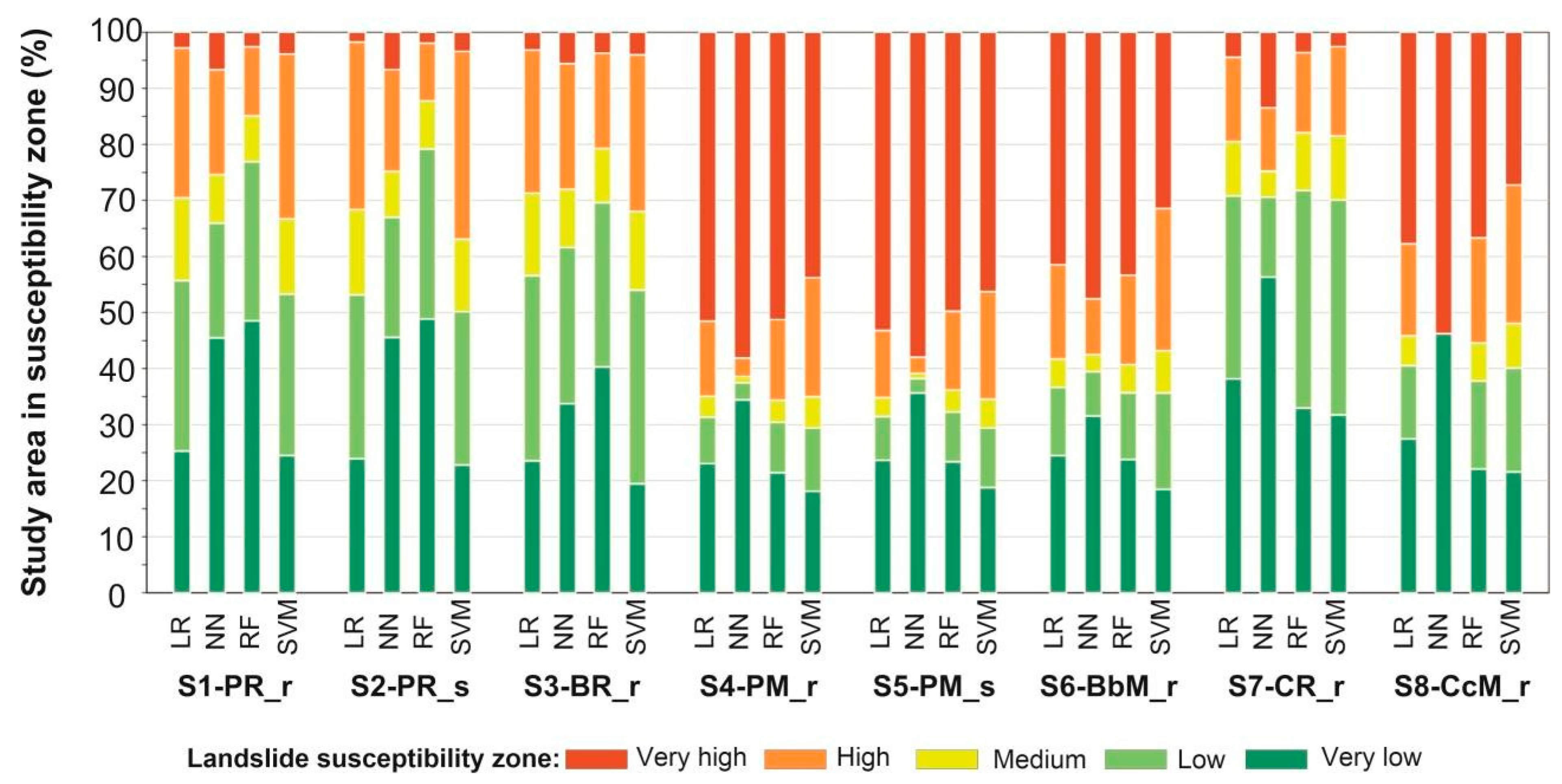
4.3. Probabilistic-Based Zonation

By observing zone area sizes (Figure 9) based on a probabilistic approach and landslide presence in each zone (Figure 10), two groups of similar results across the scenarios are identified as follows: Scenarios S1-PR_r, S2-PR_s, S3-BR_r and S7-CR_r make up one group of similar results, where very low and low zones are most present in the study area (>55%), followed by smaller area of medium and high zones and, lastly, an extremely small area of very high zones. A nearly equal distribution with approx. 70% landslide presence in very high and high zones is evident, except in scenario S7-CR_R, where the amount is roughly 50%. Consequently, scenario S7-CR_r has a significant number of landslides in the low-susceptibility zone (e.g., 30%). Scenario S4-PM_r has an extremely expressed very high zone (approximately 50%), followed by S5-PM_s, S8-CcM_r and S6-BbM_r, which comprise the second group. Very low zones are similar in size to group one, unlike low, moderate and high zones, which shrunk significantly. Landslides in the very high zone are present up to 90%, generally leaving very low and low zones with an insignificant number of landslides. This is highly expressed in scenarios S4-PM_r and S5-PM_s, and somewhat less in scenarios S6-BbM_r and S8-CcM_r.

Considering differences between LR, NN, RF and SVM methods, LR and SVM can be described as similar by showing less polarized susceptibility zones and landslide area presence. Concretely, LR and SVM models have equally expressed very low and low zones, unlike NN and RF, which have more area presence in the very low zone.

All methods depict a moderate zone 5–10% in size; however, exceptions are visible in scenarios S4-PM_r, S5-PM_s and S6-BbM_r, where the zone makes up <5% of the study area. The NN method has the largest very high zone in each scenario, followed by RF and LR. Moreover, the NN method demonstrated extreme polarization in scenario S8-CcM_r by depicting only very low and very high susceptibility zones. RF and NN methods result in nearly identical landslide presence in scenarios S4-PM_r, S5-PM_s and S6-BbM_r, whereas RF results in significantly more landslides in scenarios S1-PR_r and S2-PR_s. On the other hand, SVM and LR have only around 10% landslide presence in very high zones in scenarios S1-PR_r, S2-PR_s, S3-BR_r and S7-CR_r, indicating way higher landslide presence in high zones. Furthermore, the differences among methods in each scenario are the highest in terms of landslide presence between very high and high susceptibility zones, leaving very low, low and moderate zone areas relatively stable in each scenario. Similarly, the cumulative area of very high and high zone sizes is nearly equal in each scenario, i.e., among all methods, with the exception for RF in scenarios S1-PR_r and S2-PR_s. The LSMs classified for eight scenarios and four methods are represented in the Supplementary Material in Figures S1–S8.

5. Discussion

5.1. Model Uncertainty Considering Applied Methods and Sampling Scenarios

Considering the variability in the probabilistic susceptibility values from the derived LSMs, Figure 11 illustrates the spatial distribution and area size of the SD classes for eight sampling scenarios (Figure 11A–H) and four susceptibility methods (Figure 11I–L). Scenarios with random stable pixels showed lower deviations, i.e., S1-PR_r, S2-PR_s, S3-BR_r, and S7-CR_r, which generally account for >90% of the study area in 0.0–0.2 standard deviation classes, unlike scenarios S4-PM_r, S5-PM_s and S8-CcM_r, which account for approx. 20 or more percent of the study areas in >0.2 standard deviation classes, indicating extreme variability. It should be noted that scenario S6-BbM_r, where mapped stable pixels are used, showed greater similarity to scenarios S1-PR_r, S2-PR_s, S3-BR_r and S7-CR_r, indicating the positive influence of using unstable buffer zone pixels. Similarly, scenario S3-BR_r, which also uses buffer areas for unstable pixels, has significantly more study areas defined with the lowest SD values compared to scenarios S1-PR_r and S2-PR_s. Moreover, the difference between sampling unstable areas on regular (S1-PR_r and S4-PM_r) or smoothened (S2-PR_s and S5-PM_s) rasters resulted in negligible differences. The point sampling of unstable pixels did not significantly influence the variability, i.e., scenarios S1-PR_r and S7-CR_r showed minimal differences. On the other hand, the point sampling of unstable pixels (S8-CcM_r) increases variability, unlike the polygon sampling of unstable pixels (S4-PM_r), which showed less variability. Considering the spatial distribution, lowlands have the lowest SD values, whereas the northern part of the study area, narrowly stretching from west to east, is defined as having the highest standard deviation values, which is likely due to slope wash and other talus classes in the engineering formation LCF.

The SVM method showed the least sensitivity to sampling strategies by relating to >80% of the study area in the <0.2 standard deviation classes (Figure 11L), followed by LR, covering approx. 10% more of the study area in the 0.2–0.3 SD class (Figure 11I). SVM and LR have negligible areas present, with SD values of >0.3, unlike the RF method, which covers approx. 18% of the study area in the 0.3–0.4 SD class, mainly present in the wider-center area (Figure 11K). With >60% study area covered by >0.2 SD values, the NN method shows extreme variability in terms of sampling strategies (Figure 11J). Namely, only alluvial sediment areas and the southeastern area depicted by the limestone geological engineering unit represent low SD values when using the NN method, whereas all four methods show minimal SD values in terms of the engineering geological unit of the alluvial sediments.

5.2. Analysing Model Fitting, Predictive and Classification Performance

Considering the variability described above and the fitting, predictive and classification parameters from Section 4 (i.e., Figure 7, Figure 8, Figure 9 and Figure 10), interesting findings can be identified, as we will discuss below. The fitting performance for scenarios S1-PR_r, S2-PR_s and S3-BR_r is significantly lower compared to other scenarios, likely related to the significant number of randomly generated stable points in areas that are otherwise highly susceptible. Nonetheless, this was necessary as it ensured an unbiased approach, i.e., the model was unaware of the existence of the validation data. This is not the case for RF, which performed perfectly in all eight scenarios. On the other hand, the predictive parameters are incredibly high, meaning that all 32 models successfully classified the locations of the unseen 50% of stable and unstable polygons from the inventories. Anomalies are visible in the RF method, showing somewhat lower results compared to other methods in scenarios S1-PR_r, S2-PR_s and S3-BR_r. Perfect agreement in RF fitting performance and the anomalies in predictive performance point to overfitting behaviour. Moreover, the NN method yielded significantly lower AUC values in scenarios S7-CR_r and S8-CcM_r, indicating sensitivity to the number (i.e., points) of training pixels applied.

By comparing scenario S7-CR_r to scenarios S1-PR_r, S2-PR_s and S3-BR_r, a dispersion of landslides in all zones is evident. Namely, by changing to point sampling of unstable areas, landslides are no longer clustered in very high and high susceptibility zones but are more equally distributed, losing the purpose of the zones. Similarly, probabilistic classification can yield extremely large very high susceptibility zones (scenarios S4-PM_r, S5-PM_s, S6-BbM_r and S8-CcM_r), resulting in low landslide density, which is not expected for a very high susceptibility zone.

In terms of measuring the influence of smoothing LCFs, in scenarios S2-PR_s and S5-PM_s, negligible results are present compared to scenarios S1-PR_r and S4-PM_r, respectively. This could be because the model is less sensitive to the DTM-derived variables (elevation, slope, landform curvature, aspect, site exposure index and integrated moisture index). The latter was not addressed within the scope of this study as we opted to test the sampling strategies on a complete LCF set with no collinearity prepared to yield satisfactory AUC results. On the other hand, by having smaller low and very low zones in scenario S3-BR_r when compared to scenarios S1-PR_r and S2-PR_s, the NN and RF methods show sensitivity to the buffering of unstable areas (i.e., scenarios S3-BR_r and S6-BbM_r).

5.3. Model Verification

The predictive performance in terms of AUC and Cohen’s Kappa (Figure 8) identifies scenarios S4-PM_r, S5-PM_s, S6-BbM_r and S8-CcM_r as more favourable, and an additional AUC was calculated to investigate model applicability.

Table 6. Model verification AUC values in 32 derived LSMs.

Method	S1-PR_r	S2-PR_s	S3-BR_r	S4-PM_r	S5-PM_s	S6-BbM_r	S7-CR_r	S8-CcM_r
LR	0.790	0.772	0.754	0.683	0.662	0.690	0.737	0.696
NN	0.764	0.805	0.760	0.670	0.679	0.690	0.710	0.661
RF	0.796	0.804	0.753	0.726	0.727	0.698	0.757	0.705
SVM	0.787	0.769	0.760	0.680	0.659	0.697	0.729	0.705

depicts the model verification AUC values defined by examining the unstable validation pixels as landslide occurrences and the remaining study area as stable occurrences when considering all pixels in the entire study area. Unrealistically large very high susceptibility zones defined by a probabilistic zonation presented in Figure 9 showed scenarios S4-PM_r, S5-PM_s, S6-BbM_r and S8-CcM_r to be less favourable, which is also evident when looking to the AUC values shown in Table 6. Namely, the values correlate to poor agreement (approximately 0.7 or lower), with an exception being RF in scenarios S4-PM_r and S5-PM_s (0.726 and 0.727, respectively).

Furthermore, scenario S7-CR_r performs significantly poorer compared to scenarios S1-PR_r, S2-PR_s and S3-BR_r, whereas the NN and RF methods show the best results in scenario S2-PR_s (0.805 and 0.804, respectively). The RF method clearly stands out as having the best performance in most scenarios, followed by NN. On the other hand, NN is extremely sensitive to the sampling strategies used for stable areas (e.g., 0.661 in S8-CcM_r), as also indicated by the SD variability metric (Figure 11J). The results of scenarios S1-PR_r and S2-PR_s are relatively similar to those obtained in previous studies, i.e., [73] and [80]. Lastly, high fitting and predictive metrics can favour a sampling strategy that is opposed to reality, e.g., there are evident misclassifications by the model. It should be noted that the latter was only detectable after adding additional metrics (e.g., model verification). Scenarios S4-PM_r, S5-PM_s, S6-BbM_r and S8-CcM_r, which rely on a stable area inventory, obviously fit this misclassification category, whereas a similar effect was reported in [32], with a rectangular area limiting the stable area sampling zone to a valley. However, [32] could not quantitatively identify the misclassifying model, whereas the AUC metric presented in Table 6 proves to be a successful solution. Furthermore, as a result of experimenting with stable area sampling, overestimated high susceptibility zone issues (i.e., scenarios S4-PM_r, S5-PM_s, S6-BbM_r and S8-CcM_r in our study) were also reported in [28] and [21].

5.4. Highlighting the Unstable Centroid Sampling Disadvantages

Unstable polygon versus unstable centroid sampling proved to be a point of interest, so to further qualitatively investigate the differences, the SVM models, which demonstrated the most minor variability, were selected to compare scenarios S1-PR_r and S7-CR_r in detail (Figure 12). Figure 12A,B confirm the spatial differences in probabilistic zone sizes and landslide presence distribution for scenarios S1-PR_r and S7-CR_r, which were previously also noted (Figure 9 and Figure 10). A close up point of interest is illustrated in Figure 12C,D, based on which we conclude that centroid sampling to train the model cannot yield the probabilistic zonation which represents accurate environmental conditions, e.g., for most of the mapped landslide polygons to be present in the high and very high probabilistic zone. The following can be traced to model verification AUC (Table 6) and the landslide area presence (Figure 10), and not to the AUC parameters used for predictive performance of LSMs which are in this case misleading (generally >0.9).

6. Conclusions

This research investigates the influence of stable and unstable sampling strategies in landslide susceptibility modelling for their applicability to large-scale spatial planning systems. The modelling considered the use of eight different sampling strategies and four machine learning methods and a probabilistic zonation approach was applied. The relevant input data, i.e., spatially accurate thematic and landslide data, were carefully selected according to suggestions in the literature and previous research relating to the study area to describe local geomorphological, geological, hydrological and anthropogenic conditions in the Pannonian basin.

A novelty of this research is in the derivation of a stable areas inventory that can be used to investigate the sampling of stable pixels and smoothing of DTM-derived LCFs to capture terrain conditions before the occurrence of a landslide. The eight sampling strategies included four options for unstable pixels and stable pixels each. Namely, landslide polygon, smoothing DTM derived LCFs, polygon buffering, and landslide centroid represent four sampling strategies used for unstable pixels, whereas random points, stable area polygon, stable polygon buffering and stable area centroid were used to define the stable pixels. The processed input data were further applied in LR, NN, RF and SVM machine learning algorithms, representing commonly used methods in state-of-the-art landslide susceptibility modelling. In total, 32 LSMs were derived and analysed, considering fitting, predictive and model verification performance, as well as the SD variability for eight sampling strategies and four methods used. Furthermore, 32 zonation maps based on probabilistic zonation were described by analysing zone area, spatial distribution and landslide presence within the zones. The most significant conclusions yielded by the comprehensive comparison are as follows:

(i)

Smoothing DTM-derived LCFs at landslide locations slightly reduces model variability, whereas RF and NN models in scenario S2-PR_s using unstable polygons and randomly generated stable points represent the best LSMs

(ii)

Buffering only stable or stable and unstable polygons results in the least model variability, with a significant decline in zonation performance;

(iii)

Using the proposed stable area inventory to define stable modelling pixels by using any tested strategy drastically lowers zonation quality, which was undetectable by commonly used fitting and predictive performance metrics;

(iv)

The NN method, followed by RF, is extremely sensitive to the tested sampling strategies, whereas SVM showed the least variability, followed by similar results for LR. Additionally, with proper settings, the RF method yields LSMs that are generally better than LR, NN and SVM models;

(v)

Sampling landslides as centroids, which is extremely common in landslide susceptibility assessments, should be avoided when developing LSMs for large-scale spatial planning purposes due to the severe inability of the model to depict spatially accurate zones, which were quantitatively and qualitatively evaluated;

(vi)

A qualitative assessment of classified LSMs, quantifying zonation area size and landslide presence, represents a crucial parameter to estimate LSMs for application to large-scale spatial planning systems.

Besides the specific conclusions noted, a novelty to emphasize in terms of large-scale landslide susceptibility modelling for applicability to spatial planning systems is that commonly used quantitative metrics, i.e., Cohen’s Kappa and AUC for fitting and predictive performance, may yield misleading LSM evaluations and result in inappropriate zonation maps, e.g., poor spatial distribution when considering landslide presence. In this paper, calculating additional AUCs, i.e., model verification and qualitative assessment, enabled us to distinguish more favourable LSMs. Among the different modelling strategies, an open question remains in terms of defining a systematic approach in selecting an optimal LSM, which would consider not only the studied metrics but also take into consideration the spatial accuracy and/or susceptibility zones highlighted in this paper. Furthermore, it should be noted that large-scale landslide susceptibility models should be based on the most detailed, representative and reliable polygon-based landslide inventory possible because that will enable accurate and representative landslide susceptibility assessments and responsible and sustainable spatial planning and risk management at a local level.

References

1. Fell, R.; Corominas, J.; Bonnard, C.; Cascini, L.; Leroi, E.; Savage, W.Z. Guidelines for Landslide Susceptibility, Hazard and Risk Zoning for Land Use Planning. Eng. Geol. 2008, 102, 85–98. [Google Scholar] [CrossRef]
2. Guzzetti, F.; Reichenbach, P.; Cardinali, M.; Galli, M.; Ardizzone, F. Probabilistic Landslide Hazard Assessment at the Basin Scale. Geomorphology 2005, 72, 272–299. [Google Scholar] [CrossRef]
3. Varnes, D.J. Landslide Hazard Zonation: A Review of Principles and Practice; Education, Scientific and Cultural Organization: Paris, France, 1984. [Google Scholar]
4. Soeters, R.; van Westen, C.J. Slope Instability Recognition Analysis and Zonation. In Landslides: Investigation and Mitigation; Turner, K.T., Schuster, R.L., Eds.; National Academy Press: Washington, DC, USA, 1996; pp. 129–177. [Google Scholar]
5. Guzzetti, F.; Carrara, A.; Cardinali, M.; Reichenbach, P. Landslide Hazard Evaluation: A Review of Current Techniques and Their Application in a Multi-Scale Study, Central Italy. Geomorphology 1999, 31, 181–216. [Google Scholar] [CrossRef]
6. van Westen, C.J.; Rengers, N.; Soeters, R. Use of Geomorphological Information in Indirect Landslide Susceptibility Assessment. Nat. Hazards 2003, 30, 399–419. [Google Scholar] [CrossRef]
7. van Westen, C.J.; Castellanos, E.; Kuriakose, S.L. Spatial Data for Landslide Susceptibility, Hazard, and Vulnerability Assessment: An Overview. Eng. Geol. 2008, 102, 112–131. [Google Scholar] [CrossRef]
8. Fell, R.; Corominas, J.; Bonnard, C.; Cascini, L.; Leroi, E.; Savage, W.Z. Guidelines for Landslide Susceptibility, Hazard and Risk Zoning for Land-Use Planning. Eng. Geol. 2008, 102, 99–111. [Google Scholar] [CrossRef]
9. Corominas, J.; van Westen, C.; Frattini, P.; Cascini, L.; Malet, J.P.; Fotopoulou, S.; Catani, F.; Van Den Eeckhaut, M.; Mavrouli, O.; Agliardi, F.; et al. Recommendations for the Quantitative Analysis of Landslide Risk. Bull. Eng. Geol. Environ. 2014, 73, 209–263. [Google Scholar] [CrossRef]
10. Dias, H.C.; Hölbling, D.; Grohmann, C.H. Landslide Susceptibility Mapping in Brazil: A Review. Geosciences 2021, 11, 425. [Google Scholar] [CrossRef]
11. Das, S.; Sarkar, S.; Kanungo, D.P. A Critical Review on Landslide Susceptibility Zonation: Recent Trends, Techniques, and Practices in Indian Himalaya. Nat. Hazards 2023, 115, 23–72. [Google Scholar] [CrossRef]
12. Shano, L.; Raghuvanshi, T.K.; Meten, M. Landslide Susceptibility Evaluation and Hazard Zonation Techniques—A Review. Geoenviron. Disasters 2020, 7, 18. [Google Scholar] [CrossRef]
13. Reichenbach, P.; Rossi, M.; Malamud, B.D.; Mihir, M.; Guzzetti, F. A Review of Statistically-Based Landslide Susceptibility Models. Earth Sci. Rev. 2018, 180, 60–91. [Google Scholar] [CrossRef]
14. Pourghasemi, H.R.; Rahmati, O. Prediction of the Landslide Susceptibility: Which Algorithm, Which Precision? Catena 2018, 162, 177–192. [Google Scholar] [CrossRef]
15. Lee, S. Current and Future Status of GIS-Based Landslide Susceptibility Mapping: A Literature Review. Korean J. Remote Sens. 2019, 35, 179–193. [Google Scholar]
16. Mihalić Arbanas, S.; Bernat Gazibara, S.; Krkač, M.; Sinčić, M.; Lukačić, H.; Jagodnik, P.; Arbanas, Ž. Landslide Detection and Spatial Prediction: Application of Data and Information from Landslide Maps. In Progress in Landslide Research and Technology, Volume 1 Issue 2, 2022; Alcantara-Ayala, I., Arbanas, Ž., Huntley, D., Konagai, K., Mikoš, M., Sassa, K., Sassa, S., Tang, H., Tiwari, B., Eds.; Springer: Berlin/Heidelberg, Germany, 2023; pp. 195–212. [Google Scholar] [CrossRef]
17. Bernat Gazibara, S.; Mihalić Arbanas, S.; Sinčić, M.; Krkač, M.; Lukačić, H.; Jagodnik, P.; Arbanas, Ž. LandSlidePlan -Scientific Research Project on Landslide Susceptibility Assessment in Large Scale. In Proceedings of the Proceedings of the 5th Regional Symposium on Landslides in Adriatic—Balkan Region, Rijeka, Croatia, 23–26 March 2022; pp. 99–106. [Google Scholar]
18. Bernat, S.; Mihalić Arbanas, S.; Krkač, M. Inventory of Precipitation Triggered Landslides in the Winter of 2013 in Zagreb (Croatia, Europe). In Landslide Science for a Safer Geoenvironment; Springer International Publishing: Cham, Switzerland, 2014; pp. 829–835. [Google Scholar]
19. Sinčić, M.; Bernat Gazibara, S.; Krkač, M.; Lukačić, H.; Mihalić Arbanas, S. The Use of High-Resolution Remote Sensing Data in Preparation of Input Data for Large-Scale Landslide Hazard Assessments. Land 2022, 11, 1360. [Google Scholar] [CrossRef]
20. Krkač, M.; Bernat Gazibara, S.; Sinčić, M.; Lukačić, H.; Mihalić Arbanas, S. Landslide Inventory Mapping Based on LiDAR Data: A Case Study from Hrvatsko Zagorje (Croatia). In Proceedings of the 5th ReSyLAB, Rijeka, Croatia, 23–26 March 2022; pp. 81–86. [Google Scholar]
21. Hong, H.; Miao, Y.; Liu, J.; Zhu, A.-X. Exploring the Effects of the Design and Quantity of Absence Data on the Performance of Random Forest-Based Landslide Susceptibility Mapping. Catena 2019, 176, 45–64. [Google Scholar] [CrossRef]
22. Fu, Z.; Wang, F.; Dou, J.; Nam, K.; Ma, H. Enhanced Absence Sampling Technique for Data-Driven Landslide Susceptibility Mapping: A Case Study in Songyang County, China. Remote Sens. 2023, 15, 3345. [Google Scholar] [CrossRef]
23. Busby, J.R. Bioclim—A Bioclimatic Analysis and Prediction System. In Nature Conservation; Margules, C.R., Augstin, M.P., Eds.; CSIRO: Canberra, Australia, 1993; pp. 64–68. [Google Scholar]
24. Carpenter, G.; Gillison, A.N.; Winter, J. DOMAIN: A Flexible Modelling Procedure for Mapping Potential Distributions of Plants and Animals. Biodivers. Conserv. 1993, 2, 667–680. [Google Scholar] [CrossRef]
25. Scholkopf, G. Support Vector Method for Novelty Detection. Adv. Neural Inf. Process Syst. 2008, 12, 582–588. [Google Scholar]
26. Xiao, C.; Tian, Y.; Shi, W.; Guo, Q.; Wu, L. A New Method of Pseudo Absence Data Generation in Landslide Susceptibility Mapping with a Case Study of Shenzhen. Sci. China Technol. Sci. 2010, 53, 75–84. [Google Scholar] [CrossRef]
27. Hu, J.; Xu, K.; Wang, G.; Liu, Y.; Khan, M.A.; Mao, Y.; Zhang, M. A Novel Landslide Susceptibility Mapping Portrayed by OA- HD and K-Medoids Clustering Algorithms. Bull. Eng. Geol. Environ. 2021, 80, 765–779. [Google Scholar] [CrossRef]
28. Zhu, A.-X.; Miao, Y.; Liu, J.; Bai, S.; Zeng, C.; Ma, T.; Hong, H. A Similarity-Based Approach to Sampling Absence Data for Landslide Susceptibility Mapping Using Data-Driven Methods. Catena 2019, 183, 104188. [Google Scholar] [CrossRef]
29. Xi, C.; Han, M.; Hu, X.; Liu, B.; He, K.; Luo, G.; Cao, X. Effectiveness of Newmark-Based Sampling Strategy for Coseismic Landslide Susceptibility Mapping Using Deep Learning, Support Vector Machine, and Logistic Regression. Bull. Eng. Geol. Environ. 2022, 81, 174. [Google Scholar] [CrossRef]
30. Rabby, Y.W.; Li, Y.; Hilafu, H. An Objective Absence Data Sampling Method for Landslide Susceptibility Mapping. Sci. Rep. 2023, 13, 1740. [Google Scholar] [CrossRef] [PubMed]
31. Zhou, C.; Wang, Y.; Cao, Y.; Singhc, R.P.; Ahmed, B.; Motagh, M.; Wang, Y.; Chen, L. Non-Landslide Sampling and Ensemble Learning Techniques to Improve Landslide Susceptibility Mapping. Nat. Hazards Earth Syst. Sci. 2023. [Google Scholar] [CrossRef]
32. Lucchese, L.V.; de Oliveira, G.G.; Pedrollo, O.C. Investigation of the Influence of Nonoccurrence Sampling on Landslide Sus- ceptibility Assessment Using Artificial Neural Networks. Catena 2021, 198, 105067. [Google Scholar] [CrossRef]
33. Conoscenti, C.; Rotigliano, E.; Cama, M.; Caraballo-Arias, N.A.; Lombardo, L.; Agnesi, V. Exploring the Effect of Absence Selection on Landslide Susceptibility Models: A Case Study in Sicily, Italy. Geomorphology 2016, 261, 222–235. [Google Scholar] [CrossRef]
34. Dornik, A.; Drăguţ, L.; Oguchi, T.; Hayakawa, Y.; Micu, M. Influence of Sampling Design on Landslide Susceptibility Modeling in Lithologically Heterogeneous Areas. Sci. Rep. 2022, 12, 2106. [Google Scholar] [CrossRef]
35. Hussin, H.Y.; Zumpano, V.; Reichenbach, P.; Sterlacchini, S.; Micu, M.; van Westen, C.; Bălteanu, D. Different Landslide Sam- pling Strategies in a Grid-Based Bi-Variate Statistical Susceptibility Model. Geomorphology 2016, 253, 508–523. [Google Scholar] [CrossRef]
36. Dou, J.; Yunus, A.P.; Merghadi, A.; Shirzadi, A.; Nguyen, H.; Hussain, Y.; Avtar, R.; Chen, Y.; Pham, B.T.; Yamagishi, H. Dif- ferent Sampling Strategies for Predicting Landslide Susceptibilities Are Deemed Less Consequential with Deep Learning. Sci. Total Environ. 2020, 720, 137320. [Google Scholar] [CrossRef]
37. Huang, F.; Yan, J.; Fan, X.; Yao, C.; Huang, J.; Chen, W.; Hong, H. Uncertainty Pattern in Landslide Susceptibility Prediction Modelling: Effects of Different Landslide Boundaries and Spatial Shape Expressions. Geosci. Front. 2022, 13, 101317. [Google Scholar] [CrossRef]
38. Petschko, H.; Bell, R.; Leopold, P.; Heiss, G.; Glade, T. Landslide Inventories for Reliable Susceptibility Maps in Lower Austria. In Landslide Science and Practice; Margottini, C., Canuti, P., Sassa, K., Eds.; Springer: Berlin/Heidelberg, Germany, 2013; pp. 281–286. [Google Scholar]
39. Poli, S.; Sterlacchini, S. Landslide Representation Strategies in Susceptibility Studies Using Weights-of-Evidence Modeling Technique. Nat. Resour. Res. 2007, 16, 121–134. [Google Scholar] [CrossRef]
40. Simon, N.; Crozier, M.; de Roiste, M.; Rafek, A.G. Point Based Assessment: Selecting TheBest Way to Represent Landslide Polygon as Point Frequency in Landslide Investigation. Electron. J. Geotech. Eng. 2013, 18, 775–784. [Google Scholar]
41. Lai, J.-S.; Chiang, S.-H.; Tsai, F. Exploring Influence of Sampling Strategies on Event-Based Landslide Susceptibility Modeling. ISPRS Int. J. Geoinf. 2019, 8, 397. [Google Scholar] [CrossRef]
42. Süzen, M.L.; Doyuran, V. Data Driven Bivariate Landslide Susceptibility Assessment Using Geographical Information Systems: A Method and Application to Asarsuyu Catchment, Turkey. Eng. Geol. 2004, 71, 303–321. [Google Scholar] [CrossRef]
43. Yilmaz, I. The Effect of the Sampling Strategies on the Landslide Susceptibility Mapping by Conditional Probability and Artificial Neural Networks. Environ. Earth Sci. 2010, 60, 505–519. [Google Scholar] [CrossRef]
44. Lee, S. Landslide Susceptibility Mapping Using an Artificial Neural Network in the Gangneung Area, Korea. Int. J. Remote Sens. 2007, 28, 4763–4783. [Google Scholar] [CrossRef]
45. Yao, X.; Tham, L.G.; Dai, F.C. Landslide Susceptibility Mapping Based on Support Vector Machine: A Case Study on Natural Slopes of Hong Kong, China. Geomorphology 2008, 101, 572–582. [Google Scholar] [CrossRef]
46. Sarkar, S.; Roy, A.K.; Martha, T.R. Landslide Susceptibility Assessment Using Information Value Method in Parts of the Darjeeling Himalayas. J. Geol. Soc. India 2013, 82, 351–362. [Google Scholar] [CrossRef]
47. Hemasinghe, H.; Rangali, R.S.S.; Deshapriya, N.L.; Samarakoon, L. Landslide Susceptibility Mapping Using Logistic Regression Model (a Case Study in Badulla District, Sri Lanka). Procedia Eng. 2018, 212, 1046–1053. [Google Scholar] [CrossRef]
48. Wang, H.; Zhang, L.; Luo, H.; He, J.; Cheung, R.W.M. AI-Powered Landslide Susceptibility Assessment in Hong Kong. Eng. Geol. 2021, 288, 106103. [Google Scholar] [CrossRef]
49. Sinčić, M.; Bernat Gazibara, S.; Krkač, M.; Mihalić Arbanas, S. Landslide Susceptibility Assessment of the City of Karlovac Using Bivariate Statistical Analysis. Rudarsko-Geološko-Naftni Zb. 2022, 37, 149–170. [Google Scholar] [CrossRef]
50. Pascale, S.; Parisi, S.; Mancini, A.; Schiattarella, M.; Conforti, M.; Sole, A.; Murgante, B.; Sdao, F. Landslide Susceptibility Mapping Using Artificial Neural Network in the Urban Area of Senise and San Costantino Albanese (Basilicata, Southern Italy). Lect. Notes Comput. Sci. 2013, 7974, 473–488. [Google Scholar] [CrossRef]
51. Catani, F.; Lagomarsino, D.; Segoni, S.; Tofani, V. Landslide Susceptibility Estimation by Random Forests Technique: Sensitivity and Scaling Issues. Nat. Hazards Earth Syst. Sci. 2013, 13, 2815–2831. [Google Scholar] [CrossRef]
52. Pradhan, B. A Comparative Study on the Predictive Ability of the Decision Tree, Support Vector Machine and Neuro-Fuzzy Models in Landslide Susceptibility Mapping Using GIS. Comput. Geosci. 2013, 51, 350–365. [Google Scholar] [CrossRef]
53. Farooq, S.; Akram, M.S. Landslide Susceptibility Mapping Using Information Value Method in Jhelum Valley of the Himalayas. Arab. J. Geosci. 2021, 14, 824. [Google Scholar] [CrossRef]
54. Sandić, C.; Marjanović, M.; Abolmasov, B.; Tošić, R. Integrating Landslide Magnitude in the Susceptibility Assessment of the City of Doboj, Using Machine Learning and Heuristic Approach. J. Maps 2023, 19. [Google Scholar] [CrossRef]
55. Guo, Z.; Tian, B.; Zhu, Y.; He, J.; Zhang, T. How Do the Landslide and Non-Landslide Sampling Strategies Impact Landslide Susceptibility Assessment?—A Catchment-Scale Case Study from China. J. Rock Mech. Geotech. Eng. 2024, 16, 877–894. [Google Scholar] [CrossRef]
56. Song, Y.; Yang, D.; Wu, W.; Zhang, X.; Zhou, J.; Tian, Z.; Wang, C.; Song, Y. Evaluating Landslide Susceptibility Using Sampling Methodology and Multiple Machine Learning Models. ISPRS Int. J. Geoinf. 2023, 12, 197. [Google Scholar] [CrossRef]
57. Petschko, H.; Brenning, A.; Bell, R.; Goetz, J.; Glade, T. Assessing the Quality of Landslide Susceptibility Maps—Case Study Lower Austria. Nat. Hazards Earth Syst. Sci. 2014, 14, 95–118. [Google Scholar] [CrossRef]
58. Bornaetxea, T.; Rossi, M.; Marchesini, I.; Alvioli, M. Effective Surveyed Area and Its Role in Statistical Landslide Susceptibility Assessments. Nat. Hazards Earth Syst. Sci. 2018, 18, 2455–2469. [Google Scholar] [CrossRef]
59. Bernat Gazibara, S.; Sinčić, M.; Krkač, M.; Jagodnik, P.; Lukačić, H.; Mihalić Arbanas, S. Influence of the Landslide Inventory Completeness on the Accuracy of the Landslide Susceptibility Modelling: A Case Study from the City of Zagreb (Croatia). In Proceedings of the 6th World Landslide Forum, Florence, Italy, 14–17 November 2023; p. 644. [Google Scholar]
60. Tien Bui, D.; Tuan, T.A.; Klempe, H.; Pradhan, B.; Revhaug, I. Spatial Prediction Models for Shallow Landslide Hazards: A Comparative Assessment of the Efficacy of Support Vector Machines, Artificial Neural Networks, Kernel Logistic Regression, and Logistic Model Tree. Landslides 2016, 13, 361–378. [Google Scholar] [CrossRef]
61. Merghadi, A.; Yunus, A.P.; Dou, J.; Whiteley, J.; ThaiPham, B.; Bui, D.T.; Avtar, R.; Abderrahmane, B. Machine Learning Meth- ods for Landslide Susceptibility Studies: A Comparative Overview of Algorithm Performance. Earth Sci. Rev. 2020, 207, 103225. [Google Scholar] [CrossRef]
62. Youssef, A.M.; Pourghasemi, H.R. Landslide Susceptibility Mapping Using Machine Learning Algorithms and Comparison of Their Performance at Abha Basin, Asir Region, Saudi Arabia. Geosci. Front. 2021, 12, 639–655. [Google Scholar] [CrossRef]
63. Bernat, S.; Mihalić Arbanas, S.; Krkač, M.; Sečanj, M. Catalog of Precipitation Events That Triggered Landslides in Northwest- ern Croatia. In Proceedings of the 2nd Regional Symposium on Landslides in the Adriatic-Balkan Region, Belgrade, Serbia, 14–15 May 2015; pp. 103–107. [Google Scholar]
64. Aničić, B.; Juriša, M. Basic Geological Map, Scale 1:100,000, Rogatec, Sheet 33–68; Geological Department: Belgrade, Serbia, 1984. [Google Scholar]
65. Aničić, B.; Juriša, M. Geological Notes for Basic Geological Map, Scale 1:100,000, Rogatec, Sheet 33–68; Geological Department: Belgrade, Serbia, 1983. [Google Scholar]
66. Šimunić, A.; Pikija, M.; Hečimović, I.; Šimunić, A. Geological Notes for Basic Geological Map, Scale 1:100,000, Varaždin, Sheet 33–69; Geological Department: Belgrade, Serbia, 1982. [Google Scholar]
67. Šimunić, A.; Pikija, M.; Hečimović, I. Basic Geological Map, Scale 1:100,000, Varaždin, Sheet 33–69; Geological Department: Belgrade, Serbia, 1982. [Google Scholar]
68. Zaninović, K.; Gajić-Čapka, K.; Perčec Tadić, M.; Vučetić, M.; Milković, J.; Bajić, A.; Cindrić, K.; Cvitan, L.; Katušin, Z.; Kaučić, D. Climate Atlas of Croatia 1961–1990, 1971–2000; Croatian Meteorological and Hydrological Service: Zagreb, Croatia, 2008. [Google Scholar]
69. URL-1. Available online: https://meteo.hr/klima.php?section=klima_podaci&param=k1&Grad=varazdin (accessed on 6 June 2024).
70. Razak, K.A.; Straatsma, M.W.; van Westen, C.J.; Malet, J.P.; de Jong, S.M. Airborne Laser Scanning of Forested Landslides Characterization: Terrain Model Quality and Visualization. Geomorphology 2011, 126, 186–200. [Google Scholar] [CrossRef]
71. Bernat Gazibara, S.; Krkač, M.; Mihalić Arbanas, S. Verificiation of Historical Landslide Inventory Maps for the Podsljeme Area in the City of Zagreb Using LiDAR Based LiDAR Landslide Inventory. Rudarsko-Geološko-Naftni Zb. 2019, 34. [Google Scholar] [CrossRef]
72. Bernat Gazibara, S.; Krkač, M.; Mihalić Arbanas, S. Landslide Inventory Mapping Using LiDAR Data in the City of Zagreb (Croatia). J. Maps 2019, 15, 773–779. [Google Scholar] [CrossRef]
73. Krkač, M.; Bernat Gazibara, S.; Sinčić, M.; Lukačić, H.; Šarić, G.; Snježana, M.A. Impact of Input Data on the Quality of the Landslide Susceptibility Large-Scale Maps: A Case Study from NW Croatia. In Progress in Landslide Research and Technology; Alcánta-ra-Ayala, I., Arbanas, Ž., Cuomo, S., Huntley, D., Konagai, K., Mihalić Arbanas, S., Mikoš, M., Sassa, K., Tang, H., Tiwari, B., Eds.; Springer: Berlin/Heidelberg, Germany, 2023; pp. 135–146. [Google Scholar] [CrossRef]
74. Jagodnik, P.; Bernat Gazibara, S.; Jagodnik, V. Typed and Distribution of Quaternary Deposits Originating from Carbonate Rock Slopes in the Vinodol Valley, Croatia—New Insight Using Airborne LiDAR Data. Rudarsko-Geološko-Naftni Zb. 2020, 35, 57–77. [Google Scholar] [CrossRef]
75. Jagodnik, P.; Bernat Gazibara, S.; Arbanas, Ž.; Mihalić Arbanas, S. Engineering Geological Mapping Using Airborne LiDAR Datasets—An Example from the Vinodol Valley, Croatia. J. Maps 2020, 16, 855–866. [Google Scholar] [CrossRef]
76. URL-2. Available online: http://Geoportal.Dgu.Hr/Wms?Layers=DOF (accessed on 6 June 2024).
77. Marchesini, I.; Ardizzone, F.; Alvioli, M.; Rossi, M.; Guzzetti, F. Non-Susceptible Landslide Areas in Italy and in the Mediter- ranean Region. Nat. Hazards Earth Syst. Sci. 2014, 14, 2215–2231. [Google Scholar] [CrossRef]
78. Sinčić, M.; Bernat Gazibara, S.; Rossi, M.; Mihalić Arbanas, S. Comparison of Conditioning Factors Classification Criteria in Large Scale Statistically Based Landslide Susceptibility Models. Nat. Hazards Earth Syst. Sci. 2024. [Google Scholar] [CrossRef]
79. Evans, J.S.; Oakleaf, J.; Cushman, S.A.; Theobald, D. An Arc Gis Toolbox for Surface Gradient and Geo-Morphometric Modeling, Version 2.0-0; 2014. Available online: https://evansmurphy.wixsite.com/evansspatial/arcgis-gradient-metrics-toolbox (accessed on 1 June 2024).
80. Bernat Gazibara, S.; Sinčić, M.; Rossi, M.; Reichenbach, P.; Krkač, M.; Lukačić, H.; Jagodnik, P.; Šarić, G.; Mihalić Arbanas, S. Ap-plication of LAND-SUITE for Landslide Susceptibility Modelling Using Different Mapping Units: A Case Study in Croatia. In Progress in Landslide Research and Technology, Volume 2 Issue 2, 2023; Alcantara-Ayala, I., Arbanas, Ž., Huntley, D., Konagai, K., Mihalić Arbanas, S., Mikoš, M., Ramesh, M.V., Sassa, K., Sassa, S., Tang, H., et al., Eds.; Springer: Berlin/Heidelberg, Germany, 2023; pp. 343–354. [Google Scholar] [CrossRef]
81. Rossi, M.; Guzzetti, F.; Reichenbach, P.; Mondini, A.C.; Peruccacci, S. Optimal Landslide Susceptibility Zonation Based on Multiple Forecasts. Geomorphology 2010, 114, 129–142. [Google Scholar] [CrossRef]
82. Wang, L.-J.; Guo, M.; Sawada, K.; Lin, J.; Zhang, J. A Comparative Study of Landslide Susceptibility Maps Using Logistic Regression, Frequency Ratio, Decision Tree, Weights of Evidence and Artificial Neural Network. Geosci. J. 2016, 20, 117–136. [Google Scholar] [CrossRef]
83. The MathWorks Inc. MATLAB, Version: 9.10.0.1602886 (R2021b; The MathWorks Inc.: Natick, MA, USA, 2021; Available online: https://www.mathworks.com (accessed on 6 June 2024).
84. The MathWorks Inc. Statistics and Machine Learning, Toolbox: 12.1 (R2021); The MathWorks Inc.: Natick, MA, USA, 2021; Available online: https://www.mathworks.com/products/statistics.html (accessed on 6 June 2024).
85. URL-3. Available online: https://www.mathworks.com/help/stats/choose-a-classifier.html (accessed on 6 June 2024).
86. Gorsevski, P.V.; Gessler, P.E.; Foltz, R.B.; Elliot, W.J. Spatial Prediction of Landslide Hazard Using Logistic Regression and ROC Analysis. Trans. GIS 2006, 10, 395–415. [Google Scholar] [CrossRef]
87. Landis, J.R.; Koch, G.G. The Measurement of Observer Agreement for Categorical Data. Biometrics 1977, 159–174. [Google Scholar] [CrossRef]
88. Fawcett, T. An Introduction to ROC Analysis. Pattern Recognit. Lett. 2006, 27, 861–874. [Google Scholar] [CrossRef]
89. Rossi, M.; Reichenbach, P. LAND-SE: A Software for Statistically Based Landslide Susceptibility Zonation, Version 1.0. Geosci. Model Dev. 2016, 9, 3533–3543. [Google Scholar] [CrossRef]
90. Rossi, M.; Bornaetxea, T.; Reichenbach, P. LAND-SUITE V1.0: A Suite of Tools for Statistically Based Landslide Susceptibility Zonation. Geosci. Model Dev. 2022, 15, 5651–5666. [Google Scholar] [CrossRef]
91. Tyagi, A.; Tiwari, R.K.; James, N. Mapping the Landslide Susceptibility Considering Future Land-Use Land-Cover Scenario. Landslides 2023, 20, 65–76. [Google Scholar] [CrossRef]
92. Sweets, J.A. Measuring the Accuracy of Diagnostic Systems. Science 1988, 240, 1285–1293. [Google Scholar] [CrossRef]
Figure 2. Distributions of landslide centroids, centroids from mapped stable polygons and randomly generated stable point in different slope classes.
Remotesensing 16 02923 g002
Figure 3. Workflow for applied landslide susceptibility modelling.
Remotesensing 16 02923 g003
Figure 4. Close up examples for stable and unstable pixel sampling in training, validation and verification.
Remotesensing 16 02923 g004
Figure 5. Examples of sampling strategies: (A) polygon sampling, (B) buffer sampling and (C) smoothed LCF sampling.
Remotesensing 16 02923 g005
Figure 6. Landslide conditioning factors used in the susceptibility modelling: (A) elevation, (B) slope, (C) landform curvature, (D) aspect, (E) proximity to drainage network, (F) site exposure index, (G) integrated moisture index, (H) proximity to traffic infrastructure, (I) proximity to land use contact, (J) land use, (K) engineering formations and (L) proximity to engineering formations.
Remotesensing 16 02923 g006
Figure 7. Cohen’s Kappa and AUC fitting metrics for 32 derived landslide susceptibility models.
Remotesensing 16 02923 g007
Figure 8. Cohen’s Kappa and AUC predictive metrics for 32 derived landslide susceptibility models.
Remotesensing 16 02923 g008
Figure 9. Landslide susceptibility zone area size based on probabilistic zonation.
Remotesensing 16 02923 g009
Figure 10. Landslide area presence in susceptibility zones based on probabilistic zonation.
Remotesensing 16 02923 g010
Figure 11. Standard deviation maps of probabilistic susceptibility values for eight scenarios: (A) scenario S1-PR_r, (B) scenario S2-PR_s, (C) scenario S3-BR_r, (D) scenario S4-PM_r, (E) scenario S5-PM_s, (F) scenario S6-BbM_r, (G) scenario S7-CR_r, (H) scenario S8-CcM_r and four methods: (I) Logistic Regression, (J) Neural Network, (K) Random Forests, (L) Support Vector Machine.
Remotesensing 16 02923 g011
Figure 12. Zonation susceptibility map derived using the Support Vector Machine method in Scenarios S1-PR_r and S7-CR_r. Namely: (A,B): full extent probabilistic zonation; (C,D): close up view of probabilistic zonation.
Remotesensing 16 02923 g012