Analysis of Despeckling Filters Using Ratio Images and Divergence Measurement

Abstract

This paper presents an analysis of different despeckling filters applied on both synthetically corrupted optical images and actual Synthetic Aperture Radar (SAR) images. Several authors use optical images as ground truth and then the images are corrupted by using a Gamma model to simulate the speckle, while other approaches use methods like multitemporal fusion to generate a ground truth using actual SAR images, which provides a result somehow equivalent to the one from the common multi look technique. Well-known filters, like local, and non-local and some of them based on artificial intelligence and deep learning, are applied to these two types of images and their performance is assessed by a quantitative analysis. One last validation is performed with a newly proposed method by using ratio images, resulting from the mathematical division (Hadamard division) of filtered and noisy images, to measure how similar the initial and the remaining speckle are by considering its Gamma distribution and divergence measurement. Our findings suggest that despeckling models relying on artificial intelligence exhibit notable efficiency, albeit concurrently displaying inflexibility when applied to particular image types based on the training dataset. Additionally, our experiments underscore the utility of the divergence measurement in ratio images in facilitating both visual inspection and quantitative evaluation of residual speckles within the filtered images.

1. Introduction

SAR is a technology that uses active sensors to obtain high-resolution data from the Earth’s surface, by sending microwave signals to the target area and then processing the backscattered signal to generate images from the surface [1]. One of the main advantages of using SAR imagery is the ability to obtain data day and night despite the environmental conditions since the microwave signal can be measured through clouds, smoke, fog, rain, snow and even penetrate the ground [2]. 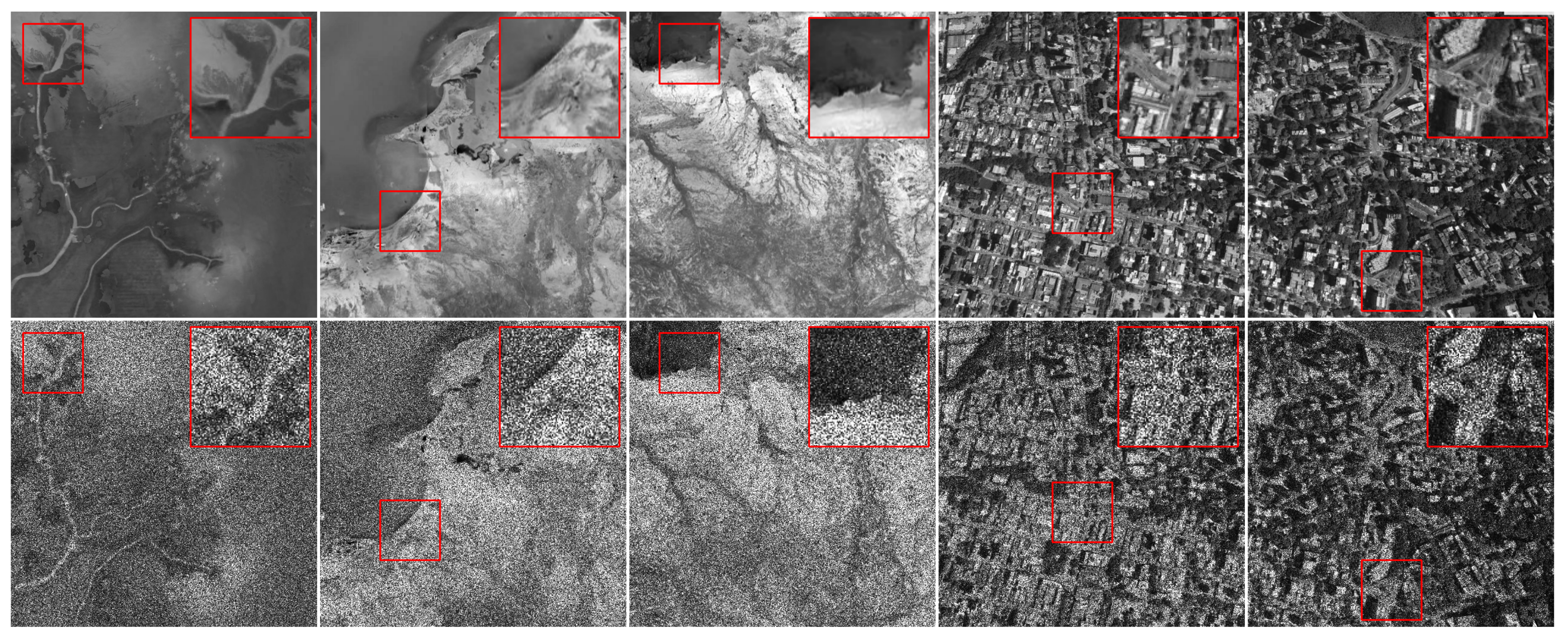One of the main disadvantages of the SAR technology is the speckle, a granular pattern present in all these types of images, that limits the availability of labeled datasets with ground-truth images to train supervised artificial intelligence models [3], or to assessing the quality of the filtering process by comparing two images (ground truth and filtered). So, many authors use synthetically corrupted optical images with speckles and use the optical images as ground truth and the corrupted images as simulated SAR to be filtered. For this reason, it is very common that different publications assess the quality of the despeckling processes by using the optical reference, but when they are tested on actual SAR images there is no ground truth reference and the metrics and measurements cannot be calculated [4,5].

To quantitatively evaluate the despeckling process in SAR images, various metrics are utilized. One such metric is the Equivalent Number of Looks (ENL), which measures the noise level in a single image and is calculated as the square of the mean pixel value in a homogeneous region divided by the square of the standard deviation in the same region. The Mean Squared Error (MSE) assesses the average squared differences between two images’ pixel values, with a lower MSE indicating higher similarity [6]. The Structural Similarity Index (SSIM) evaluates the similarity between two images in terms of luminance, contrast, and structure, with values close to 1 indicating high structural similarity. The Peak Signal-to-Noise Ratio (PSNR) quantifies the reconstruction quality of lossy compression codecs; higher PSNR values denote better filtering quality [7]. Pratt’s Figure of Merit (PFOM) measures the accuracy of edge detection by comparing real and extracted edges in two images, with values close to 1 indicating perfect similarity in edge detection [8]. The correlation measure proposed in [9] and used in [10] is a comprehensive indicator of despeckling quality since it uses edge detection to measure the correlation between two images. This $\beta$ edge estimator was adapted in [11] by including a radio edge detector to measure the geometric content remaining in a ratio image, called the $\alpha \beta$-Ratio estimator. The $\mathcal{M}$-estimator in [12] proposes that an evaluation based on a statistical measure of the quality of the remaining speckle is the first-order component of the quality measure.

In [13] it is asserted that methodologies trained on synthetic datasets often exhibit subpar performance in practical applications, primarily attributable to the lack of clean SAR images. As a remedy, an innovative unsupervised despeckling technique, integrating online speckle generation with unpaired training, is introduced. In [14] the construction of a diverse and authentic dataset utilizing a multicategory generalized Gaussian coherent SAR simulator is described. A markedly distinct methodology has recently surfaced [15,16,17], wherein an enhanced SAR dataset is derived through the multitemporal averaging of SAR images to achieve a more authentic reference image.

In [18] a novel protocol was introduced. This protocol involves generating ground truth data through the multitemporal fusion of multiple images depicting the same scene. This approach facilitated the creation of a labeled dataset and the training of new Deep Learning (DL) models aimed at reducing speckle noise using actual SAR images. This opens a new possibility to assess the quality of despeckling techniques applied to these actual SAR images. The main advantage of this protocol is the design of a labeled dataset with ground truth reference, which was split to train and validate the DL despeckling model.

The despeckling of SAR images employs a variety of filters to reduce speckle noise while preserving important image features. The traditional Lee filter adjusts the number of neighboring pixels within the sliding window to improve performance [19]. The Fast Adaptive Nonlocal SAR (FANS) filter evolves from SAR-BM3D, utilizing nonlocal filtering and wavelet-domain shrinkage, with modifications tailored to SAR image characteristics, achieving superior results in terms of signal-to-noise ratio and perceived image quality [20]. Among AI-based filters, the Autoencoder (AE) compresses and decompresses images through convolutional layers, effectively reducing noise during this process [18,21]. The multi-objective network (MONet) incorporates a modified cost function with the Kullback–Leibler divergence, demonstrating improved performance in metrics such as SSIM, SNR, and MSE over various nonlocal filters [15]. The Semantic Conditional U-Net (SCUNet) combines semantic segmentation and image denoising in a unified framework, using an encoder-decoder structure with semantic information conditioning to enhance feature extraction and noise reduction [22].

The innovative aspect of this paper lies in its comprehensive evaluation of traditional and AI-based despeckling filters applied to both synthetically corrupted optical images and actual SAR images using a novel method involving ratio images to measure residual speckles. Unlike prior studies that often rely solely on synthetically corrupted data or multitemporal fusion for ground truth, this work introduces a divergence measurement approach to quantitatively and visually assess the similarity between initial and remaining speckle. This method provides a more robust framework for evaluating the effectiveness of despeckling techniques, particularly highlighting the flexibility and limitations of AI-based models when applied to real-world SAR imagery. Additionally, the study underscores the importance of gamma distribution approximation in understanding the behavior of residual speckles, offering new insights and tools for future research in SAR image despeckling.

This paper is organized as follows. In Section 2, the materials are presented, including the datasets used and the description of the metrics to assess the quality of the despeckling process. In Section 3, the Speckle model and the proposed method to assess the despeckling processes are explained. In Section 4 the experiments and measurements are presented, including all the processing steps, both on actual SAR and optical images. In Section 5 a discussion and interpretation of the results is presented. Finally, in Section 6 some relevant conclusions and future work are outlined.

2. Materials

2.1. Optical Dataset

Optical images were obtained from Google Earth, each of them corrupted with synthetic speckle, following (10). First, $ENL=2.0$, the values are similar to the ones found in Sentinel-1 SAR imagery, as shown in Figure 1.

2.2. SAR Dataset

SAR imagery was obtained from satellite SAR sensors and their corresponding platforms to download data from different dates. From the downloaded data, it is possible to rescale, register, crop and label the datasets. Then, a despeckling process was applied to these datasets, by using different filters, including state-of-the-art ones, with DL architectures, in order to measure its performance and compare its results. One novelty in this analysis is the use of actual SAR imagery, departing from designed datasets by performing a multitemporal fusion of SAR data to generate the ground truth. Sentinel-1 represents the initial mission within the five-part series that the European Space Agency (ESA) is developing for the Copernicus initiative. It consists of a constellation of two polar-orbiting satellites (A and B) designed to operate day and night with a revisiting period of 6 days at a height of 693 km from Ecuador [23].

The Sentinel-1 data utilized in this study were downloaded from [24] in intensity mode level “L1 Single Look Complex (SLC)”, C band at 5.4 GHz with a resolution of 10 m, VV and VH polarizations. The images correspond to the region of Toronto in 2024, since it is heterogeneous and includes vegetation, urban areas and man-made structures like bridges, buildings and highways. Based on the protocol proposed in [18], ten Sentinel-1 images of the same location were downloaded from this region. These images were rescaled, registered, averaged and cropped in order to obtain a new despeckled ground truth reference, a process that provides a result somehow equivalent to the one from the common multi-look technique. The software used in this generation was Sentinel Application Platform (SNAP) from the European Space Agency (ESA), carefully preserving the float format.

In order to assess the effectiveness of the despeckling process, datasets need to be annotated with ground truth (reference) and SAR images, arranged in pairs as outlined in [25], where the available dataset is composed of: 1500 SAR noisy images for training, 100 SAR noisy images for validation, 1500 noiseless (ground truth) images for training, and 100 noiseless (ground truth) images for validation. The dataset comprises two folders, namely ’Ground Truth’ and ’Noisy’ which correspond to the noiseless and actual SAR images, respectively, as shown in Figure 2.

2.3. Metrics

A quantitative evaluation of the despeckling process is necessary to assess the quality of the resulting despeckled images. There are metrics that have been widely used by performing operations in single images to calculate individual measurements in the whole image or regions of interest inside it, or by using two images to compare by using mathematical or statistical operations.

2.3.1. Equivalent Number of Looks

The Equivalent Number of Looks (ENL) is a measurement of the level of noise in a single image. An image with a higher ENL is a less noisy image. It is calculated from the square of the mean of the pixels inside a homogeneous region, divided by the square of the standard deviation in the same region, according to (1).

$$ENL={\displaystyle \frac{{\mu }^2}{{\sigma }^2}}$$

(1)

2.3.2. Mean Squared Error

The Mean Squared Error (MSE) is a value calculated from the averaged squared errors pixel by pixel between two images. A larger MSE indicates more different images, while an MSE close to zero indicates that the images are very similar in their pixel values. The MSE is calculated according to (2).

$$MSE={\displaystyle \frac{1}{N}}\sum _{i=0}^{m-1}\sum _{j=0}^{n-1}{(Y(i,j)-Z(i,j))}^2.$$

(2)

2.3.3. Structural Similarity Index

The Structural Similarity Index (SSIM) is a measurement of the similarity between two images by using three terms: luminance, contrast, and structure. The SSIM index is calculated using according to (3). Values of SSIM equal or close to 0 indicate no structural similarity, while values close to 1 indicate higher structural similarity.

$$SSIM(x,y)={\displaystyle \frac{(2{\mu }_x{\mu }_y+c_1)·(2{\sigma }_{xy}+c_2)}{({\mu }_x^2+{\mu }_y^2+c_1)·({\sigma }_x^2+{\sigma }_y^2+c_2)}},$$

(3)

where ${\mu }_x$ and ${\mu }_y$ are the average pixel values of images x and y, respectively, ${\sigma }_x$ and ${\sigma }_y$ are the standard deviations of x and y, ${\sigma }_{xy}$ is the covariance between x and y, and $c_1$ and $c_2$ are constants to stabilize the division.

2.3.4. Peak Signal-to-Noise Ratio

The Peak Signal-to-Noise Ratio (PSNR) is a measurement of the quality of reconstruction of lossy compression codecs. It is defined as the division between the maximum possible power of a signal and the power of corrupting noise. Higher values of PSNR indicate a better filtering process and it is calculated according to (4).

$$PSNR=10·{log}_{10}\left({\displaystyle \frac{MA{X}^2}{MSE}}\right),$$

(4)

where $MAX$ is the maximum possible pixel value of the images.

2.3.5. Beta

Beta is a quantitative measurement of the edge preservation in images, defined in [10] according to (5).

$$\beta ={\displaystyle \frac{\Gamma (\Delta S-\overline{\Delta S},\widehat{\Delta S}-\overline{\widehat{\Delta S}})}{\sqrt{\Gamma (\Delta S-\overline{\Delta S},\Delta S-\overline{\Delta S})·\Gamma (\widehat{\Delta S}-\overline{\widehat{\Delta S}},\Delta S-\overline{\widehat{\Delta S}}}}},$$

(5)

where $\Delta S$ and $\widehat{\Delta S}$ are the high-pass filtered versions of S and $\widehat{S}$, respectively, and $\Gamma$ is the Laplacian operator.

2.3.6. Pratt’s Figure of Merit

Pratt’s Figure Of Merit (PFOM) is a measurement of the accuracy of edge detection by comparing real and extracted edges in two images and the distances between the found edges [8]. Values of 0 indicate low similarity, while values of 1 indicate perfect similarity. The PFOM is calculated according to (6).

$$PFOM={\displaystyle \frac{1}{max(I_l,I_A))}}\sum _{i=1}^{I_A}{\displaystyle \frac{1}{1+{\alpha }_f\times d^2\left(i\right)}},$$

(6)

where $I_A$ and $I_l$ determine points of real edges and extracted edges, $d\left(i\right)$ is the distance between $i^{th}$ point on the image with estimated edges and the nearest edge point on the real image, and ${\alpha }_f$ is usually fixed at $1/9$.

2.4. Despeckling Filters

Although the first filtering algorithms were proposed more than 30 years ago, the despeckling of SAR images is still an open issue [26]. Speckle suppression aims to smooth the homogeneous regions while preserving edge and texture in the image [27]. In the seminal work [28] a protocol is proposed in which optical (natural) images are considered as noiseless data and then, using a speckle model-like form, for example, a Gamma distribution law, these images are corrupted to simulate the speckle. This way, both the noiseless and the speckled images are available and can be evaluated through different metrics. These traditional filters are not based on artificial intelligence, since they use mathematics and statistics exclusively to model and attenuate the speckle. They can be divided into local and nonlocal filters. Nonlocal filters replace the value of a pixel with the average of similar pixels that have no reason to be spatially close [29].

2.4.1. Lee Filter

The well-known Lee filter [30] can be considered the most traditional SAR despeckling approach. Its output is given by (7):

$$I_{ij}^{Lee}={\overline{I}}_{ij}+{\displaystyle \frac{{\sigma }_{ij}^2}{I_{ij}^{-2}{\sigma }_{\mu }^2+{\sigma }_{ij}^2}}(I_{ij}-{\overline{I}}_{ij}),$$

(7)

where $I_{ij}^{Lee}$ is the output image, ${\overline{I}}_{ij}$ denotes the local mean in the scanning window centered on the ij-th pixel, $I_{ij}$ denotes the central element in the window, and ${\sigma }_{ij}^2$ is the variance of the pixel values in the current window.

This filter has had modifications like the Enhanced Lee Filter (ELee) that improve the performance of the original filter, by preserving information and details of the original image [31].

2.4.2. FANS Filter

The Fast Adaptive Nonlocal SAR (FANS) despeckling filter is an evolution on the SAR-BM3D [20] which is based on the concepts of nonlocal filtering and wavelet-domain shrinkage for additive white Gaussian noise denoising, with a modification in its processing steps to consider the peculiarities of the SAR images. FANS include a probabilistic similarity measure and wavelet shrinkage to look for the optimum local linear minimum-mean-square-error estimator in the wavelet domain. This makes FANS perform better than other state-of-the-art reference techniques, specifically in terms of signal-to-noise ratio (on simulated speckled images) and of perceived image quality.

2.5. AI-Based Filters

In recent years, there has been an increase in research exploring the application of AI techniques for speckle reduction in SAR imagery. Unlike traditional methods that exclusively use mathematical and statistical models, AI-based filters leverage more advanced machine learning algorithms to learn and adapt to complex patterns present in images. These approaches offer promising capabilities to effectively mitigate speckle while preserving important SAR imagery features. This subsection explores several prominent AI-based filtering techniques and their performance in speckle removal.

2.5.1. MONET

The model for SAR despeckling called multi-objective network (MONet) proposed in [15] uses a modified cost function that includes the Kullback–Leibler divergence. This model has improved results based on the metrics SSIM, SNR, and MSE over nonlocal filters like NOLAND, ID-CNN, SAR-DRN, SARBM3D, and even FANS. The complete cost function includes a linear combination of three terms according to (8), each of them specifically dedicated to catching and preserving information from the SAR image.

$$\mathcal{L}={\mathcal{L}}_2+{\lambda }_{KL}{\mathcal{L}}_{KL}+{\lambda }_{\Delta }{\mathcal{L}}_{\Delta },$$

(8)

where ${\mathcal{L}}_2={\mathcal{L}}_{MSE}={∥\widehat{X}-X∥}^2$ is the MSE between the reference X and the filtered image $\widehat{X}$, ${\mathcal{L}}_{KL}=D_{KL}(\widehat{N},N_{teo})$ is the Kullback–Leibler divergence ($D_{KL}$) between the distribution of estimated noise $\widehat{N}$ and the theoretical one $N_{teo}$, ${\mathcal{L}}_{\Delta }={∥\nabla X-\nabla \widehat{X}∥}^2$ is the MSE between the gradient of the reference X and the gradient of the filtered image $\widehat{X}$.

2.5.2. Autoencoder

An Autoencoder (AE) is a type of artificial neural network used to learn efficient codings of images. It has convolutional layers that compress (encoder) the images to a smaller size and then recover the images to their original size (decoder). During this process, the noise is eliminated or attenuated, making it a deep-learning model for despeckling. The AE used in this work was adapted from [21] as defined and trained in [18] composed of input as the noisy image, which in this case is a clip of $512\times 512\times 1$. The encoder is a layer of 32 convolutional 2D filters with RELU activation followed by a downsampling MaxPooling operation along its spatial dimensions (height and width) by taking the maximum value over an input window of size $2\times 2$. Again, another layer of 32 filters of 2D filters followed by a MaxPooling operation of size 2 × 2. The Latent layer, or bottleneck, has the image transformed with the smallest dimensions ($128\times 128$), one-fourth of the input size. The Decoder is composed of two layers of transposed convolution, also called “deconvolution” of 32 filters. Finally, one layer consists of one last 2D convolution filter of size $3\times 3$. The Output is a layer that delivers a new grayscale image, resulting from the compression and decompression of the autoencoder, a process in which the noise is reduced. The output has the same size of $512\times 512\times 1$.

2.5.3. Semantic Conditional U-Net

The Semantic Conditional U-Net (SCUNet) is a deep learning architecture proposed for SAR imagery despeckling tasks [22] that integrates both semantic segmentation and image denoising into a unified framework, allowing for simultaneous feature extraction and noise reduction. The architectural framework consists of an encoder-decoder structure, similar to the U-Net, augmented with semantic information conditioning. This conditioning is achieved through the incorporation of additional semantic segmentation maps as input, providing contextual guidance for the denoising process. SCUNet leverages a combination of convolutional and transposed convolutional layers for feature extraction and upsampling, facilitating noise suppression while preserving important SAR imagery features.

3. Experimental Methodology

3.1. Speckle Model

The Multiplicative Model is just one of the infinitely many ways to build stochastic descriptions for SAR data. One of its advantages is that it can be considered an ab initio model, and that it leads to expressive and tractable descriptions of the data. According to this model, a SAR image Y can be expressed as (9):

$$Y=X·N,$$

(9)

where X is the noise-free image and N is the speckle noise, which has distribution characterized by the density:

$$f_Z(z;L,{\sigma }^2)={\displaystyle \frac{L^L}{{\sigma }^{2L}\Gamma \left(L\right)}}{z}^{L-1}{e}^{-Lz/{\sigma }^2},$$

(10)

where L is the Equivalent Number of Looks (ENL) of the SAR image and $\Gamma \left(L\right)$ is the Gamma distribution [32]. For simplicity and ease of implementation in programming languages, $a=L$ and $b={\sigma }^2/a$, (10) can be rewritten as (11):

$$f_Z(z;a,b)={\displaystyle \frac{1}{b^a\Gamma \left(a\right)}}{z}^{a-1}{e}^{z/b}.$$

(11)

The Gamma distribution is scale-invariant, and this model can be posed as the product between the constant backscatter $X={\sigma }^2$ and the multilook speckle $Y=\Gamma (1,L)$. However, there are situations where constant backscatter results from infinitely many elementary backscatterers. Such an assumption makes the particular choice of the sensed area irrelevant. The advent of higher-resolution sensors makes this hypothesis unsuitable in areas where the elementary backscatterers are of the order of the wavelength. If, for instance, we are dealing with a 1 m × 1 m resolution image, we may consider many elementary backscatterers if the target is flat and composed of grass; if the target is a forest, this assumption may be unrealistic. Other models like Kappa, Reciprocal Gamma, and Inverse Gaussian distributions for SAR images are considered in [32].

3.2. Ratio Analysis

A filtered SAR image $\widehat{X}$ will resemble its noise-free reference X depending on the performance of the filter. Assuming the multiplicative model in (9), in order to evaluate how the filters perform, different metrics have been proposed in the literature. Also, the ratio images have been used [12,26,33]. A ratio image can be calculated as the pixel-wise division of the observed SAR image Y and the filtered image $\widehat{X}$ (12):

$$\widehat{N}={\displaystyle \frac{Y}{\widehat{X}}}.$$

(12)

A homogeneous region of this ratio image $\widehat{N}$ must have a Gamma distribution that can be compared to the analytic Gamma distribution. Our proposal is that the divergence between these distributions is an indicator of the quality of the despeckling process.

The measurement used in this paper is the Jensen–Shannon Divergence (JSD) [34,35] according to (13):

$$L(P,Q)=H(aP+(1-a\left)Q\right)-aH\left(P\right)-(1-a)H\left(Q\right),$$

(13)

where $H\left(P\right)$ is the Shanon entropy.

In the ideal case having two equal distributions, the $JSD=0$, while cases with disparities in these distributions show higher $JSD$ values. A visual inspection of the first- and second-order statistics is also useful for assessing the quality of the despeckling process: the former checks marginal properties, while the latter verifies lack of structure [12].

3.3. Proposed Analysis

The proposed experimental analysis consists of obtaining images of two types: optical and actual SAR. Optical images are considered the ground truth and the noisy samples are generated with synthetic noise by using a Gamma distribution with different number of looks. In the case of SAR data, these actual images are considered noisy, and several images from the same region of different dates are used to generate the noise-free (ground truth) reference.

All the images are despeckled by using six filters: Lee, ELee, and FANS are not AI-based, while the other three: MONET, AE, and SCUNet are DL-based. The resulting filtered images are evaluated by using well-known metrics: ENL, MSE, SSIM, PSNR, beta and PFOM. Finally, our proposal is to assess the Gamma approximation of the resulting ratio of a filtered image by comparing it with respect to the observed image (SAR or synthetically corrupted optical). Also, visual inspection is performed on all the resulting images.

4. Results

4.1. Despeckling Process

The despeckling processes were performed by using all the filters and then evaluated by using the metrics described in Section 2. All the filters preserved the original size of $512\times 512$ of the noisy images.

4.2. Measurements in Optical Images

A homogeneous region of $20\times 20$ every image was selected to calculate the equivalent number of looks (ENL), including ground truth, SAR (noisy) and filtered images (

Table 1. Measurement of ENL in synthetically speckled and filtered images from the optical samples.

ENL	1	2	3	4	5
Noisy	1.73	2.42	1.91	1.56	2.15
Ground Truth	360.22	1523.36	577.69	7.37	63.53
Lee	69.90	19.76	79.66	15.45	38.76
ELee	104.03	97.85	142.38	12.03	107.73
FANS	552.89	425.07	1001.71	11.11	938.25
MONET	30.20	27.84	63.49	6.64	22.71
AE	16.51	24.18	51.27	5.93	35.96
SCUNet	1.99	1.93	1.61	1.21	1.76

), then the ground truth and the filtered images were compared to calculate the MSE (

Table 2. Measurement of MSE in synthetically speckled and filtered images from the optical samples.

MSE	1	2	3	4	5
Noisy	5382.65	9820.74	11,654.75	5500.09	3779.98
Lee	154.15	821.72	644.87	7650.81	822.27
ELee	156.65	339.99	539.29	897.40	671.79
FANS	78.41	217.66	415.36	629.30	457.19
MONET	721.82	918.54	1007.02	877.47	709.66
AE	850.70	1590.64	1677.88	1178.68	805.10
SCUNet	3996.93	5129.55	5340.56	3343.83	2399.65

), the SSIM (

Table 3. Measurement of SSIM in synthetically speckled and filtered images from the optical samples.

SSIM	1	2	3	4	5
Noisy	0.03	0.04	0.06	0.27	0.30
Lee	0.58	0.29	0.35	0.08	0.50
ELee	0.57	0.45	0.37	0.39	0.49
FANS	0.82	0.63	0.41	0.57	0.61
MONET	0.23	0.24	0.29	0.57	0.59
AE	0.22	0.22	0.30	0.55	0.57
SCUNet	0.04	0.05	0.09	0.33	0.36

), the PSNR (

Table 4. Measurement of PSNR in synthetically speckled and filtered images from the optical samples.

PSNR	1	2	3	4	5
Noisy	10.82	8.21	7.47	10.73	12.36
Lee	26.25	18.98	20.04	9.29	18.98
ELee	26.18	22.82	20.81	18.60	19.86
FANS	29.19	24.75	21.95	20.14	21.53
MONET	19.55	18.50	18.10	18.70	19.62
AE	18.83	16.12	15.88	17.42	19.07
SCUNet	12.11	11.03	10.85	12.89	14.33

), the beta (

Table 5. Measurement of Beta in synthetically speckled and filtered images from the optical samples.

BETA	1	2	3	4	5
Noisy	0.009	0.009	0.013	0.119	0.145
Lee	0.041	0.039	0.026	0.010	0.179
ELee	0.042	0.059	0.032	0.064	0.136
FANS	0.122	0.089	0.030	0.205	0.216
MONET	0.012	0.023	0.043	0.201	0.214
AE	0.016	0.023	0.052	0.165	0.171
SCUNet	0.012	0.021	0.034	0.169	0.177

), and the PFOM (

Table 6. Measurement of PFOM in synthetically speckled and filtered images from the optical samples.

PFOM	1	2	3	4	5
Noisy	0.29	0.40	0.57	0.70	0.70
Lee	0.49	0.62	0.73	0.79	0.85
E_Lee	0.50	0.77	0.76	0.77	0.81
FANS	0.56	0.60	0.54	0.80	0.83
MONET	0.33	0.51	0.73	0.81	0.80
AE	0.36	0.54	0.77	0.85	0.85
SCUNet	0.30	0.40	0.59	0.73	0.74

). The best results were also highlighted in bold formatting, while the second-position results were underlined. The resulting images when the same six filters were applied are shown in Figure 3.

Table 1 displays the ENL values measured in synthetically speckled and filtered images from optical samples. Five samples (denoted as 1 to 5) were evaluated under different conditions: the initial noisy image, the ground truth image, and the images filtered using six different methods (Lee, ELee, FANS, MONET, AE, and SCUNet). The results indicate that the ground truth image has the highest ENL values, signifying lower noise levels, particularly notable in samples 2 and 3. Among the filtering methods, FANS achieved the best results in most samples, standing out in samples 1, 3, and 5. The SCUNet filter showed lower performance in terms of ENL compared to the other methods evaluated.

Table 2 presents the MSE measurements obtained from synthetically speckled and filtered images derived from optical samples. The MSE values reflect the discrepancy between the filtered images and the ground truth, with lower values indicating higher similarity. Among the filters, FANS achieved the lowest MSE values across all the samples, indicating its effectiveness in reducing noise and preserving image fidelity. Conversely, SCUNet exhibited higher MSE values, suggesting comparatively poorer performance in noise reduction.

Table 3 displays the SSIM measurements obtained from synthetically speckled and filtered images derived from optical samples. The SSIM values range between 0 and 1, where higher values indicate greater similarity between the filtered images and the ground truth. Notably, FANS achieved the highest SSIM values across all the samples, indicating its superior ability to preserve structural information while reducing noise. Conversely, SCUNet generally exhibited lower SSIM values, suggesting comparatively less effective noise reduction and preservation of image structure.

Table 4 presents the PSNR measurements for synthetically speckled and filtered images derived from optical samples. PSNR values indicate the quality of the filtered images compared to the ground truth, with higher values reflecting better image fidelity. Notably, FANS consistently achieved the highest PSNR values across all samples, indicating superior noise reduction and preservation of image quality. Conversely, SCUNet exhibited lower PSNR values, suggesting comparatively less effective noise reduction and image fidelity preservation.

Table 5 shows the $\beta$ measurement for optical images, demonstrating the superiority of the FANS filter in four out of the five samples, and the AE in one of them. Table 6 displays the PFOM measurements for synthetically speckled and filtered images derived from optical samples. PFOM values represent the performance of different filtering techniques in preserving image features and reducing noise. Higher PFOM values indicate better preservation of image features and higher image fidelity. Notably, the AE filter achieved the highest PFOM values across most samples, indicating superior performance in preserving image features. Conversely, SCUNet exhibited relatively lower PFOM values compared to other filters, suggesting less effective preservation of image features.

The ratio images were obtained following (12). Ratio images are supposed to be pure speckle after an ideal despeckling process; however, this is not the case with the filters available in the literature. One region of interest in each of these images was approximated to a Gamma distribution following (10), The resulting ratio images for these regions of interest are shown in Figure 4. The analysis of distributions of the analytic speckle generated with the number of looks measured in the noisy image and the Gamma distribution found in the ratio image is shown in Figure 5. The measurement of the JSD in the five optical samples is shown in

Table 7. Measurement of JSD in five optical samples.

JSD	1	2	3	4	5
Lee	0.0039	0.0042	0.0005	0.0007	0.0027
E_Lee	0.0059	0.0037	0.0006	0.0010	0.0012
FANS	0.0059	0.0027	0.0008	0.0011	0.0018
MONET	0.0139	0.0036	0.0219	0.0025	0.0016
AE	0.0072	0.0041	0.0059	0.0025	0.0002
SCUNet	0.0289	0.0535	0.0567	0.0542	0.0421

.

4.3. Measurements in Filtered SAR Images

A homogeneous region of $20\times 20$ every image was selected to calculate the equivalent number of looks (ENL), including ground truth, SAR (noisy) and filtered images (

Table 8. Measurement of ENL in SAR, ground truth and filtered images from the Sentinel-1 dataset.

ENL	1	2	3	4	5
Noisy	2.03	1.79	1.84	1.30	1.53
Ground Truth	13.87	15.85	18.26	4.79	11.22
Lee	106.25	38.92	60.47	6.92	91.84
ELee	134.03	67.69	100.40	6.99	116.95
FANS	452.83	431.86	943.26	6.61	873.49
MONET	14.87	8.78	8.91	3.69	7.94
AE	27.07	24.34	132.17	10.32	29.43
SCUNet	1.41	0.74	0.93	0.44	0.88

). Then, all SAR and filtered images were compared with respect to the ground truth reference, by calculating the MSE (

Table 9. Measurement of MSE in SAR, ground truth and filtered images from the Sentinel-1 dataset.

MSE	1	2	3	4	5
Noisy	5098.08	3952.50	3146.29	4685.04	5108.18
Lee	3446.15	2945.54	2093.63	3486.97	2678.61
ELee	3479.35	2973.16	2110.03	3498.84	2682.75
FANS	2957.37	2322.60	1754.92	2704.85	2486.55
MONET	2736.56	2266.30	1769.29	2575.63	2351.19
AE	2573.02	2081.44	1684.80	2499.90	2305.62
SCUNet	5905.80	4551.18	3460.59	5338.80	5906.17

), the SSIM (

Table 10. Measurement of SSIM in SAR and filtered images with respect to ground truth from the Sentinel-1 dataset.

SSIM	1	2	3	4	5
Noisy	0.38	0.39	0.38	0.44	0.25
Lee	0.19	0.22	0.39	0.14	0.11
ELee	0.17	0.22	0.39	0.12	0.11
FANS	0.26	0.34	0.47	0.34	0.14
MONET	0.38	0.44	0.49	0.46	0.29
AE	0.39	0.43	0.49	0.42	0.27
SCUNet	0.38	0.38	0.39	0.42	0.23

), the PSNR (

Table 11. Measurement of PSNR in SAR and filtered images with respect to ground truth from the Sentinel-1 dataset.

PSNR	1	2	3	4	5
Noisy	11.06	12.15	13.14	11.41	11.05
Lee	12.76	13.44	14.91	12.71	13.84
ELee	12.72	13.39	14.89	12.69	13.85
FANS	13.41	14.46	15.69	13.81	14.16
MONET	13.76	14.58	15.64	14.01	14.42
AE	14.03	14.95	15.87	14.14	14.50
SCUNet	10.42	11.55	12.74	10.86	10.42

), the beta (

Table 12. Measurement of Beta in SAR and filtered images with respect to ground truth from the Sentinel-1 dataset.

BETA	1	2	3	4	5
Noisy	0.307	0.375	0.331	0.305	0.186
Lee	0.068	0.044	0.082	0.017	0.007
ELee	0.042	0.036	0.059	0.014	0.003
FANS	0.216	0.269	0.229	0.217	0.100
MONET	0.287	0.336	0.296	0.279	0.195
AE	0.296	0.334	0.279	0.247	0.149
SCUNet	0.298	0.367	0.326	0.299	0.180

), and the PFOM (

Table 13. Measurement of PFOM in SAR and filtered images with respect to ground truth from the Sentinel-1 dataset.

PFOM	1	2	3	4	5
Noisy	0.81	0.80	0.86	0.82	0.72
Lee	0.72	0.76	0.80	0.75	0.76
E_Lee	0.72	0.76	0.78	0.75	0.77
FANS	0.70	0.78	0.73	0.76	0.66
MONET	0.83	0.88	0.86	0.89	0.79
AE	0.88	0.89	0.89	0.89	0.85
SCUNet	0.81	0.82	0.86	0.83	0.73

). The best result of every sample is shown in bold formatting, while the second position result is shown underlined. The resulting filtered images are shown in Figure 6.

Table 8 presents the ENL measurements for SAR images, ground truth, and filtered images from the Sentinel-1 dataset. The ENL values, which reflect the noise reduction performance and image quality, are shown for various filtering techniques. The FANS filter consistently achieved the highest ENL values across most samples, indicating superior noise reduction and image quality enhancement. Other filters, such as ELee and AE, also showed notable improvements compared to the noisy images, while SCUNet had the lowest ENL values, suggesting less effective noise reduction in this context.

Table 9 displays the MSE measurements for SAR images, ground truth, and filtered images from the Sentinel-1 dataset. The MSE values, which indicate the pixel-wise difference between the filtered images and the ground truth, are shown for various filtering techniques. The AE filter consistently achieved the lowest MSE values across all samples, suggesting superior accuracy in noise reduction. Other filters like MONET and FANS also performed well, with relatively low MSE values compared to the noisy images. SCUNet had the highest MSE values, indicating less effective performance in this context.

Table 10 presents the SSIM measurements for SAR and filtered images compared to the ground truth from the Sentinel-1 dataset. The SSIM values, which indicate the similarity between the filtered images and the ground truth, are reported for different filtering methods. The MONET filter achieved the highest SSIM scores for most samples, indicating a strong resemblance to the ground truth. The AE filter also performed well, with SSIM values close to those of MONET. The noisy images had varying SSIM values, generally lower than those of the best-performing filters.

Table 11 displays the PSNR measurements for SAR and filtered images compared to the ground truth from the Sentinel-1 dataset. The PSNR values, which measure the quality of the filtered images in relation to the ground truth, are reported for various filtering methods. The AE filter achieved the highest PSNR scores across all samples, indicating superior image quality. MONET and FANS also performed well, with MONET consistently securing the second-best scores. The noisy images had the lowest PSNR values, highlighting the improvement achieved through filtering.

Table 12 shows $\beta$ measurements for actual SAR-filtered images with respect to the ground truth from the Sentinel-1 dataset. In this case, the best preservation appeared in the noisy images, except in the fifth sample, where MONET obtained the best result. Table 13 presents the PFOM measurements for these same images. The AE filter consistently achieved the highest PFOM values across all samples, indicating the best performance. MONET also performed well, frequently securing the second-highest scores. The noisy images showed varying PFOM values, generally lower than the filtered images, demonstrating the effectiveness of the filtering methods.

The resulting ratio images for the actual SAR samples are shown in Figure 7. The analysis of distributions of the analytic speckle generated with the number of looks measured in the noisy image and the Gamma distribution found in the ratio image is shown in Figure 8. The measurement of the JSD in the five SAR samples is shown in

Table 14. Measurement of JSD in five SAR samples.

JSD	1	2	3	4	5
Lee	0.0000	0.0079	0.0095	0.0303	0.0116
E_Lee	0.0001	0.0051	0.0059	0.0282	0.0103
FANS	0.0001	0.0032	0.0035	0.0450	0.0096
MONET	0.0204	0.0433	0.0327	0.1013	0.0753
AE	0.0048	0.0167	0.0399	0.0464	0.0247
SCUNet	0.1371	0.2005	0.1781	0.2177	0.1627

.

5. Discussion

5.1. Optical Imagery

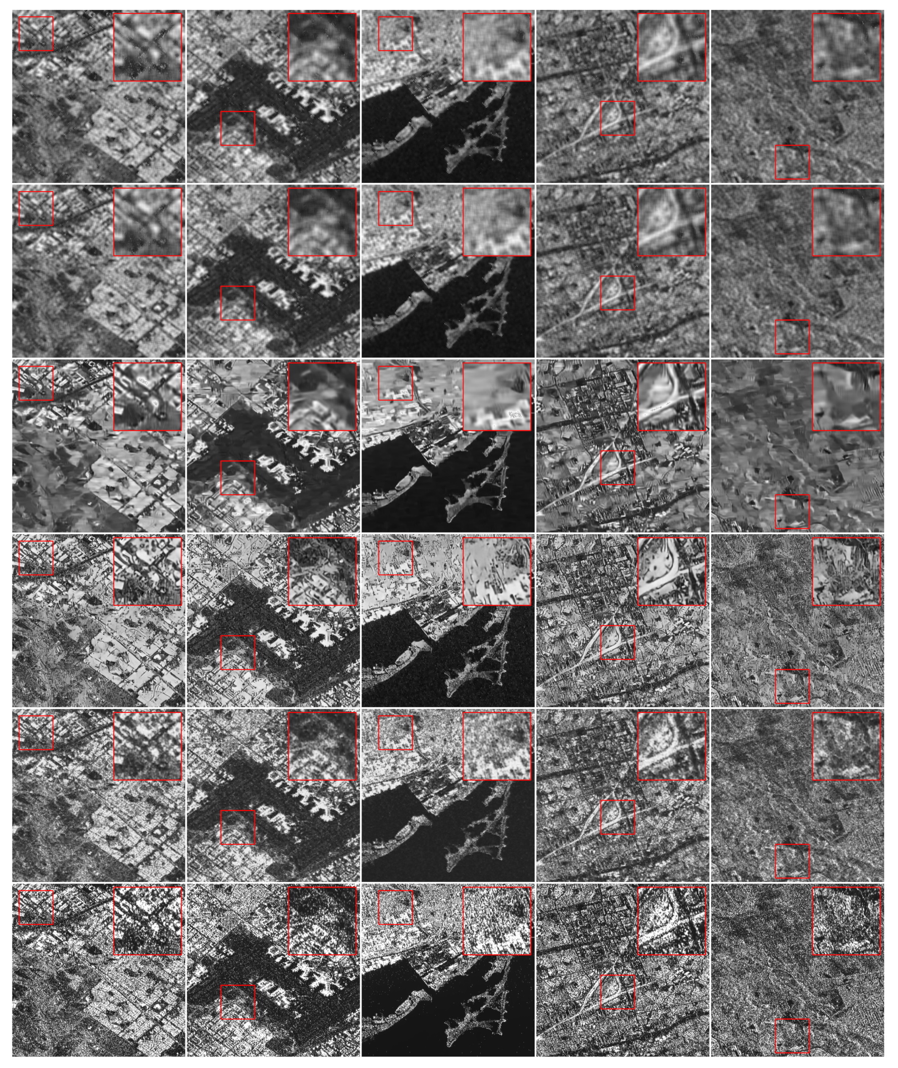
All the despeckling filters increased the ENL compared to the noisy image. The FANS filter exceeded the ENL observed in the ground truth images (Table 1), which is undesirable as it indicates an over-smoothing effect, which can be confirmed in the third row of Figure 3. The other filters remained within adequate limits, with the exception of SCUNet, which did not perform adequately in the optical dataset. It must be noticed that the FANS algorithm requires the number of looks as an input parameter when executed, so this could explain the adaptability that DL-based models lack.

The measurements of the MSE in Table 2 represent the difference between the filtered images and the ground truth, with lower values indicating higher similarity. FANS consistently achieved the lowest MSE across most samples, demonstrating its effectiveness in preserving image details while reducing noise. SCUNet, conversely, showed higher MSE values, suggesting it was less effective in maintaining image fidelity.

SSIM (Table 3) values range from 0 to 1, with higher values indicating greater similarity to the ground truth. FANS again performed the best, achieving the highest SSIM values across most samples. This indicates that FANS not only reduced noise effectively but also preserved the structural information of the images. SCUNet exhibited lower SSIM values, highlighting its comparative inefficiency in maintaining structural integrity during noise reduction.

PSNR (Table 4) values indicate the quality of the filtered images, with higher values reflecting better image fidelity. FANS achieved the highest PSNR values across most samples, indicating its superior performance in noise reduction and image quality preservation. In contrast, SCUNet showed lower PSNR values, reinforcing the observations from the MSE and SSIM metrics regarding its lower effectiveness.

PFOM (Table 6) values assess the filters’ performance in preserving image features while reducing noise. Higher PFOM values indicate better preservation of image features. The AE filter achieved the highest PFOM values in most samples, suggesting its excellent performance in feature preservation. FANS also performed well, consistently achieving high PFOM values, while SCUNet again showed relatively lower PFOM values, indicating less effective feature preservation.

The measurements of the MSE (Table 2), SSIM (Table 3), and PSNR (Table 4) confirm the previous analysis, with FANS being the best in these metrics with optical images. The preservation of edges indicated by the PFOM (Table 6) shows the AE has the best results in three out of the five samples.

In Table 7, it is observed that the Jensen–Shannon Divergence (JSD) index of the Lee method performed the best in images 1, 3, and 4. However, the Lee method did not exhibit significant performance in terms of speckle suppression or edge preservation when compared to other filters. This discrepancy can be explained by the inherent characteristics of the JSD index and the nature of the Lee filter.

The JSD index focuses on the statistical preservation of noise characteristics rather than visual quality. The Lee filter may excel in maintaining the statistical properties of the speckle noise, resulting in low JSD values. However, this does not necessarily translate to effective speckle suppression or edge preservation, which are critical for visual quality and structural integrity.

The Lee filter’s performance is particularly strong in homogeneous regions where it can accurately preserve the local statistics. In such areas, the ratio image’s speckle remains close to the theoretical distribution, resulting in a lower JSD. This might explain its superior JSD performance in images 1, 3, and 4 if these images contain significant homogeneous regions. The Lee filter tends to blur edges and fine details because it averages pixel values within the local window. This limitation affects its performance in edge preservation and visual quality metrics like beta and PFOM, despite its ability to preserve the statistical properties of the speckle.

5.2. Actual SAR Imagery

Similarly to the optical case, all despeckling filters applied to the SAR dataset increased the ENL compared to the noisy image (Table 8). Once again, the FANS filter exhibited the highest increase in ENL, indicating an over-smoothing effect, as demonstrated in the third row of Figure 6. SCUNet struggled to adapt to the noise characteristics in these images, suggesting it was trained on a substantially different dataset, resulting in a rigid despeckling process.

Other metrics, such as MSE, SSIM, PSNR, beta and PFOM (Table 9, Table 10, Table 11, Table 12 and Table 13, respectively), consistently indicate that the AE model outperforms other filters. This superior performance is attributable to the AE model’s ability to accurately represent the characteristics of speckle noise, as it was trained on a dataset comprising actual SAR images.

Table 9 displays MSE measures the difference between filtered images and ground truth. The AE filter consistently achieved the lowest MSE values across all samples, suggesting superior accuracy in noise reduction. Conversely, SCUNet had the highest MSE values, indicating less effective performance. The low MSE of AE suggests that this filter is highly accurate in approximating ground truth, surpassing other filters in precision. The relationship between AE and MONET is notable, as both show low MSE values, indicating they are good at preserving important details while reducing noise.

Table 10 presents SSIM measures structural similarity between filtered images and ground truth. The MONET filter achieved the highest SSIM scores for most samples, indicating a strong resemblance to ground truth. AE also performed well, with SSIM values close to those of MONET. The relationship between MONET and AE is particularly interesting, as both filters not only reduce noise but also preserve image structure. This suggests that both filters are effective not only in noise reduction but also in preserving crucial structural information of SAR images.

Table 11 displays PSNR measures image quality relative to ground truth. The AE filter consistently achieved the highest PSNR scores across all samples, indicating superior image quality. The high PSNR of AE reinforces its effectiveness in improving image quality, corroborating MSE and SSIM results. The relationship between AE and MONET again is notable, showing that both filters not only preserve image structure but also significantly improve overall image quality.

Table 13 presents PFOM indicates the degree of similarity between filtered images and ground truth. The AE filter consistently achieved the highest PFOM values, indicating the best performance. The consistency of AE in achieving the highest PFOM values suggests that it is the most effective filter in terms of improving overall image quality compared to ground truth. The relationship between AE and MONET shows that both filters are effective in improving image quality and similarity to ground truth.

5.3. Analysis of Gamma and Divergence in Ratio Images

In theory, ratio images should exhibit pure speckle under ideal conditions. However, after the application of a practical filter to a noisy image, patterns, structures and shapes persist within the resultant ratio image. The Gamma distribution obtained from the theoretical noise contrasted with the one obtained from the ratio image indeed exhibits disparities, measured through the JSD. This proposed methodology is a second-order measurement, that must be applied only when first-order evaluations are performed and the despeckling quality is found to be suitable. Scenarios such as in Figure 7 where the last row corresponding to SCUNet exhibited the absence of structure as residual information corroborates this recommendation. This holds true despite the fact that the mean was not preserved and the metrics are suboptimal when compared to the other filters.

The ratio images JSD values observed for the optical dataset in Figure 4 and Figure 5, and for the SAR dataset in Figure 7 and Figure 8 exhibit behavior consistent with a Gamma distribution. These results highlight the expected differences between the analytically added and observed noise and the noise measured in the ratio images.

The JSD values documented in Table 7, Table 8, Table 9, Table 10, Table 11, Table 12, Table 13 and Table 14 align with observations derived from Gamma distributions. Certain filters, such as SCUNet, demonstrate challenges in accurately modeling the inherent randomness of the speckle. These results are further corroborated by the ratio images depicted in Figure 4, Figure 5, Figure 6 and Figure 7, where the images that display structures and shapes correspond to the ones with higher JSD values.

5.4. Evaluation of Methodology

The methodology employed in this study involves an evaluation of traditional and AI-based despeckling filters using both synthetically corrupted optical images and actual SAR images. This dual approach allows for a robust assessment of the filter performance across different types of data, which is crucial for understanding their practical applicability.

5.4.1. Analysis

The use of synthetic speckle on optical images provides a controlled environment to evaluate the filters, allowing for clear comparisons against known ground truth data. This method is appropriate as it enables the assessment of how well filters can remove speckle noise without sacrificing image details. The synthetic approach is particularly beneficial in initial testing phases, where controlled conditions are necessary to benchmark different techniques.

In addition to synthetic data, the study incorporates actual SAR images, ensuring that the findings are relevant to real-world scenarios. The multitemporal fusion technique used to generate ground truth references from SAR images is a notable strength of this methodology. This technique enhances the reliability of the ground truth by averaging multiple images of the same scene, which effectively reduces the noise inherent in individual SAR images. This approach is appropriate as it provides a realistic benchmark for evaluating despeckling filters in practical applications.

However, there are potential limitations to this methodology. Firstly, while the synthetic speckle approach allows for controlled comparisons, it may not capture all the complexities and variabilities present in actual SAR images. Real-world SAR data often contain additional noise sources and artifacts that are not fully replicated in synthetic scenarios. This limitation suggests that while synthetic tests are useful, they should be complemented by extensive testing on actual SAR data.

Another limitation is the reliance on multitemporal fusion to create ground truth references for SAR images. This method assumes that the scene remains unchanged across the multiple images used for fusion. Any changes in the scene (e.g., due to temporal dynamics) could introduce inaccuracies in the ground truth, potentially affecting the evaluation of despeckling performance. Therefore, while this approach is robust for many applications, it may not be suitable for highly dynamic environments where the scene changes significantly over time.

Additionally, the evaluation metrics used in the study, such as ENL, MSE, SSIM, PSNR, beta and PFOM, provide valuable quantitative assessments of filter performance. However, these metrics have their own limitations and might not capture all aspects of the visual quality and usability of the despeckled images. Future research could benefit from incorporating subjective assessments or additional metrics that better reflect the perceptual quality of the images.

5.4.2. Appropriateness and Limitations of AI-Based Models

AI-based models have shown significant promise in this study. These models leverage large datasets to learn complex patterns in speckle noise and effectively remove it while preserving image details. The flexibility of these models allows them to adapt to different noise characteristics, which is a major advantage over traditional methods.

However, AI-based models also have limitations. Their performance heavily depends on the quality and diversity of the training data. If the training data do not adequately represent the variety of scenarios encountered in actual SAR applications, the models may not generalize well. Additionally, AI models require substantial computational resources for training and may be sensitive to the choice of hyperparameters.

5.5. Feedback on Analysis

The analysis conducted in this study provides an evaluation of the despeckling filters, utilizing both quantitative metrics and qualitative visual inspections. The inclusion of multiple metrics such as ENL, MSE, SSIM, PSNR, beta, and PFOM offers a well-rounded assessment of filter performance, while the ratio analysis and divergence measurement provide innovative methods for evaluating residual speckle.

5.5.1. Strengths of the Analysis

Comprehensive Metrics: The use of multiple metrics ensures that different aspects of filter performance are captured. Metrics like SSIM and PSNR evaluate image quality and structural similarity, while ENL focuses on noise reduction effectiveness.

Dual Data Sources: By employing both synthetically corrupted optical images and actual SAR images, the study covers a wide range of scenarios. This dual approach strengthens the validity of the findings, as it shows how filters perform in controlled and real-world conditions.

Ratio Analysis and Divergence Measurement: These innovative methods provide a deeper understanding of residual speckle and its distribution, offering a new perspective on despeckling filter evaluation. The use of Gamma distribution approximation and Jensen–Shannon Divergence (JSD) adds robustness to the analysis.

5.5.2. Areas for Improvement

Subjective quality assessment: While quantitative metrics are essential, incorporating subjective quality assessments through user studies could provide additional insights. Human perception of image quality often differs from what metrics capture, and subjective assessments can highlight aspects of filter performance that metrics might miss.

Temporal dynamics in SAR images: The current methodology assumes static scenes for multitemporal fusion. Future studies should explore methods to account for temporal dynamics in SAR images, ensuring that ground truth generation remains accurate even in changing environments. This could involve advanced techniques for detecting and compensating for changes in the scene.

Real-world application scenarios: While the study provides a solid foundation, further research should investigate the performance of despeckling filters in specific real-world applications. For example, how do these filters impact subsequent tasks such as object detection, classification, or change detection in SAR imagery? Evaluating filters in the context of these applications would provide practical insights into their utility.

5.6. Implications and Contributions to the Literature

The findings from this study have several important implications for the field of SAR image despeckling. By comprehensively evaluating both traditional and AI-based despeckling filters, the study provides a robust framework for understanding their strengths and limitations. The key implications of the findings are as follows:

Efficacy of AI-based filters: The study demonstrates that AI-based filters, such as Autoencoder (AE) and Multi-Objective Network (MONET), can achieve superior performance in noise reduction and image quality preservation compared to traditional filters. This highlights the potential of AI techniques in advancing despeckling methodologies and sets a new benchmark for future research.

Importance of dataset diversity: The performance of AI-based filters heavily depends on the quality and diversity of the training datasets. The findings underscore the necessity for diverse and comprehensive training datasets that adequately represent the variability in real-world SAR imagery. This has implications for the design and curation of training datasets in future studies.

Ratio analysis and divergence measurement: The innovative use of ratio images and divergence measurement provides a novel method for evaluating residual speckle. This approach offers a more detailed understanding of speckle behavior post-filtering and can be used as a supplementary evaluation metric in future despeckling research.

Flexibility of traditional filters: Traditional filters like FANS showed adaptability across different types of images, performing well in both optical and actual SAR datasets. This flexibility is valuable for applications where AI-based models may not be feasible due to computational constraints or a lack of suitable training data.

This study makes several significant contributions to the existing literature on despeckling filters:

Comprehensive evaluation framework: By integrating both traditional and AI-based filters and employing a wide range of evaluation metrics, the study provides a comprehensive framework for assessing despeckling techniques. This holistic approach can serve as a reference for future studies aiming to evaluate and compare despeckling filters.

Novel analytical techniques: The introduction of ratio analysis and divergence measurement as tools for evaluating residual speckle represents a novel contribution to the field. These techniques offer new insights into the behavior of despeckled images and can complement traditional evaluation metrics in providing a more nuanced understanding of filter performance.

Benchmarking AI-based models: The study benchmarks several state-of-the-art AI-based despeckling models, providing detailed performance evaluations. This contributes to the growing body of literature on the application of AI in SAR image processing and highlights the potential and challenges of these techniques.

Insights into speckle behavior: The findings provide deeper insights into the behavior of speckle noise in SAR imagery and the effectiveness of different despeckling techniques. This contributes to the theoretical understanding of speckle noise and offers practical guidance for researchers and practitioners working on SAR image analysis.

Guidance for future research: The study identifies key areas for improvement and future research, such as the need for diverse training datasets, the exploration of hybrid filtering approaches, and the development of advanced ground truth generation techniques. These insights can guide future research efforts in the field.

6. Conclusions and Future Work

The protocol to generate a ground truth from a multitemporal fusion of SAR images allowed to have a dataset containing ground truth images to serve as a reference when assessing the quality of the despeckling filters. In the case of optical images, the original ones served as a reference while the synthetically corrupted ones served as noisy pairs.

Across all evaluated metrics, FANS emerged as the most effective filtering method for reducing noise and preserving image fidelity and structural integrity in synthetically speckled optical images. SCUNet, while less effective across these metrics, highlights the variability in the performance of different filtering methods. The AE filter, although not always the best in noise reduction, demonstrated strong performance in preserving important image features. These results underscore the importance of selecting appropriate filtering methods based on the specific requirements of image processing tasks.

The results of various evaluation metrics show that filters AE and MONET excel in multiple aspects. AE leads in terms of MSE, PSNR, beta, and PFOM, demonstrating precision and quality in noise reduction. MONET, on the other hand, exhibits high preservation of image structure, achieving the best results in SSIM and performing well in PSNR and PFOM. The FANS filter demonstrates extreme effectiveness in noise reduction according to ENL but may not be the best for maintaining image quality in terms of SSIM and PSNR. SCUNet, though less effective compared to other filters, shows mixed performance that may be useful in specific contexts. These in-depth analyses provide insight into the strengths and weaknesses of each filter, offering a solid foundation for selecting the most suitable filter based on specific SAR image processing needs.

The DL-based models are very efficient when applied on specific images, for instance, the AE outperforms actual SAR images, but it does not stand out when applied on optical ones, and the SCUNet was not able to attenuate the synthetic speckle added by using a Gamma model. On the other hand, the FANS filter could adapt to different levels of speckle and obtain better results in both, SAR and optical images.

The experiments conducted underscore the utility of ratio analysis in facilitating both visual inspection and quantitative evaluation of residual speckle within the filtered images. This innovative approach provides a comprehensive tool for understanding and assessing the efficacy of despeckling techniques in SAR images, enabling a direct comparison between the initial and residual speckle. By combining visual analysis and quantitative metrics, the study offers a more complete understanding of the effects of despeckling filters, allowing for a more precise assessment of their performance across different conditions and types of images. This approach has significant implications for the ongoing improvement of despeckling techniques and their application in a variety of contexts.

The proposed method of analysis of ratio images and divergence measurement is in line with the results derived from the other well-known metrics also calculated in this paper for both types of images. This is also in concordance with the findings after visually inspecting the filtered images.

Future research can be focused on using other levels of SAR imagery, or SAR data obtained from other satellites like RadarSAT or TerraSAR-X, which will require the design of new datasets by using a methodology similar to the one used in this work. Also, it can be possible to include more metrics to assess the despeckling quality. Other works may focus on improving the ratio analysis based on the Gamma approximation proposed in this paper.

The methodology used in this study is robust and appropriate for evaluating the effectiveness of despeckling filters. While there are potential limitations, such as the synthetic nature of some tests and the assumptions in multitemporal fusion, the approach provides a comprehensive framework for assessing both traditional and AI-based despeckling techniques. Future research should aim to address these limitations by incorporating more diverse datasets and exploring additional evaluation metrics.

Future Work

Adapting AI models to diverse data: AI-based models should be trained on more diverse and comprehensive datasets to improve their generalization capabilities. Research could focus on transfer learning techniques to adapt models trained on one type of data to perform well on another.

Exploring hybrid approaches: Combining traditional and AI-based methods could leverage the strengths of both approaches. For instance, using traditional filters to preprocess data before applying AI models might improve overall performance.

Advanced ground truth generation techniques: Developing more sophisticated methods for ground truth generation in SAR imagery, especially in dynamic environments, would enhance the reliability of despeckling filter evaluations.

Real-time despeckling: Researching methods to optimize despeckling filters for real-time processing could expand their applicability in operational settings, where timely data analysis is critical.

References

1. Wei, S.; Zeng, X.; Qu, Q.; Wang, M.; Su, H.; Shi, J. HRSID: A high-resolution SAR images dataset for ship detection and instance segmentation. IEEE Access 2020, 8, 120234–120254. [Google Scholar] [CrossRef]
2. Singh, P.; Diwakar, M.; Shankar, A.; Shree, R.; Kumar, M. A Review on SAR Image and its Despeckling. Arch. Comput. Methods Eng. 2021, 28, 4633–4653. [Google Scholar] [CrossRef]
3. Argenti, F.; Lapini, A.; Bianchi, T.; Alparone, L. A Tutorial on Speckle Reduction in Synthetic Aperture Radar Images. IEEE Geosci. Remote Sens. Mag. 2013, 1, 6–35. [Google Scholar] [CrossRef]
4. Cozzolino, D.; Verdoliva, L.; Scarpa, G.; Poggi, G. Nonlocal CNN SAR image despeckling. Remote Sens. 2020, 12, 1006. [Google Scholar] [CrossRef]
5. Yuan, Y.; Guan, J.; Feng, P.; Wu, Y. A practical solution for SAR despeckling with adversarial learning generated speckled-to-speckled images. IEEE Geosci. Remote Sens. Lett. 2020, 19, 1–5. [Google Scholar] [CrossRef]
6. Jain, V.; Shitole, S.; Rahman, M. Performance evaluation of DFT based speckle reduction framework for synthetic aperture radar (SAR) images at different frequencies and image regions. Remote Sens. Appl. Soc. Environ. 2023, 31, 101001. [Google Scholar] [CrossRef]
7. Mullissa, A.G.; Marcos, D.; Tuia, D.; Herold, M.; Reiche, J. DeSpeckNet: Generalizing deep learning-based SAR image despeckling. IEEE Trans. Geosci. Remote Sens. 2020, 60, 1–15. [Google Scholar] [CrossRef]
8. Balochian, S.; Baloochian, H. Edge detection on noisy images using Prewitt operator and fractional order differentiation. Multimed. Tools Appl. 2022, 81, 9759–9770. [Google Scholar] [CrossRef]
9. Sattar, F.; Floreby, L.; Salomonsson, G.; Lövström, B. Image enhancement based on a nonlinear multiscale method. IEEE Trans. Image Process. Publ. IEEE Signal Process. Soc. 1997, 6, 888–895. [Google Scholar] [CrossRef]
10. Achim, A.M.; Kuruoğlu, E.E.; Zerubia, J. SAR image filtering based on the heavy-tailed Rayleigh model. IEEE Trans. Image Process. 2006, 15, 2686–2693. [Google Scholar] [CrossRef] [PubMed]
11. Déniz, L.G.; Buemi, M.E.; Jacobo-Berlles, J.; Mejail, M. A New Image Quality Index for Objectively Evaluating Despeckling Filtering in SAR Images. IEEE J. Sel. Top. Appl. Earth Obs. Remote Sens. 2016, 9, 1297–1307. [Google Scholar]
12. Déniz, L.G.; Ospina, R.; Frery, A.C. Unassisted Quantitative Evaluation of Despeckling Filters. Remote Sens. 2017, 9, 389. [Google Scholar] [CrossRef]
13. Wang, C.; Zheng, R.; Zhu, J.W.; He, X.; Li, X. Unsupervised SAR Despeckling by Combining Online Speckle Generation and Unpaired Training. IEEE J. Sel. Top. Appl. Earth Obs. Remote Sens. 2023, 16, 10175–10190. [Google Scholar] [CrossRef]
14. Vitale, S.; Ferraioli, G.; Frery, A.C.; Pascazio, V.; Yue, D.X.; Xu, F. SAR Despeckling Using Multiobjective Neural Network Trained With Generic Statistical Samples. IEEE Trans. Geosci. Remote Sens. 2023, 61, 1–12. [Google Scholar] [CrossRef]
15. Vitale, S.; Ferraioli, G.; Pascazio, V. Multi-Objective CNN-Based Algorithm for SAR Despeckling. IEEE Trans. Geosci. Remote Sens. 2020, 59, 9336–9349. [Google Scholar] [CrossRef]
16. Cozzolino, D.; Verdoliva, L.; Scarpa, G.; Poggi, G. Nonlocal SAR Image Despeckling by Convolutional Neural Networks. In Proceedings of the IGARSS 2019—2019 IEEE International Geoscience and Remote Sensing Symposium, Yokohama, Japan, 28 July–2 August 2019; pp. 5117–5120. [Google Scholar]
17. Chierchia, G.; Cozzolino, D.; Poggi, G.; Verdoliva, L. SAR image despeckling through convolutional neural networks. In Proceedings of the 2017 IEEE International Geoscience and Remote Sensing Symposium (IGARSS), Fort Worth, TX, USA, 23–28 July 2017; pp. 5438–5441. [Google Scholar] [CrossRef]
18. Vásquez-Salazar, R.D.; Cardona-Mesa, A.A.; Gómez, L.; Travieso-González, C.M. A New Methodology for Assessing SAR Despeckling Filters. IEEE Geosci. Remote Sens. Lett. 2024, 21, 1–5. [Google Scholar] [CrossRef]
19. Yommy, A.S.; Liu, R.; Wu, S. SAR Image Despeckling Using Refined Lee Filter. In Proceedings of the 2015 7th International Conference on Intelligent Human-Machine Systems and Cybernetics, Hangzhou, China, 26–27 August 2015; Volume 2, pp. 260–265. [Google Scholar] [CrossRef]
20. Parrilli, S.; Poderico, M.; Angelino, C.V.; Verdoliva, L. A Nonlocal SAR Image Denoising Algorithm Based on LLMMSE Wavelet Shrinkage. IEEE Trans. Geosci. Remote Sens. 2012, 50, 606–616. [Google Scholar] [CrossRef]
21. Valderrama, S.L. Keras Documentation: Convolutional Autoencoder for Image Denoising. 2021. Available online: https://keras.io/examples/vision/autoencoder/ (accessed on 5 March 2024).
22. Wang, W.; Kang, Y.; Liu, G.; Wang, X. SCU-net: Semantic segmentation network for learning channel information on remote sensing images. Comput. Intell. Neurosci. 2022, 2022, 8469415. [Google Scholar] [CrossRef]
23. ESA. Sentinel-1 Missions. 2023. Available online: https://sentiwiki.copernicus.eu/web/s1-mission (accessed on 5 March 2024).
24. NASA. ASF Data Search. 2023. Available online: https://search.asf.alaska.edu/ (accessed on 5 March 2024).
25. Vásquez-Salazar, R.D.; Cardona-Mesa, A.A.; Gómez, L.; Travieso-González, C.M.; Garavito-González, A.F.; Vásquez-Cano, E. Labeled dataset for training despeckling filters for SAR imagery. Data Brief 2024, 53, 110065. [Google Scholar] [CrossRef]
26. Ferraioli, G.; Pascazio, V.; Schirinzi, G. Ratio-Based Nonlocal Anisotropic Despeckling Approach for SAR Images. IEEE Trans. Geosci. Remote Sens. 2019, 57, 7785–7798. [Google Scholar] [CrossRef]
27. Li, J.; Wang, Z.; Yu, W.; Luo, Y.; Yu, Z. A Novel Speckle Suppression Method with Quantitative Combination of Total Variation and Anisotropic Diffusion PDE Model. Remote Sens. 2022, 14, 796. [Google Scholar] [CrossRef]
28. Lee, J.S.; Jurkevich, L.; Dewaele, P.; Wambacq, P.; Oosterlinck, A. Speckle filtering of synthetic aperture radar images: A review. Remote Sens. Rev. 1994, 8, 313–340. [Google Scholar] [CrossRef]
29. Buades, A.; Coll, B.; Morel, J.M. Non-Local Means Denoising. Image Process. Online 2011, 1, 208–212. [Google Scholar] [CrossRef]
30. Lee, J.S. Digital image enhancement and noise filtering by use of local statistics. IEEE Trans. Pattern Anal. Mach. Intell. 1980, PAMI-2, 165–168. [Google Scholar] [CrossRef]
31. Rubel, O.S.; Lukin, V.V.; Rubel, A.; Egiazarian, K.O. Selection of Lee Filter Window Size Based on Despeckling Efficiency Prediction for Sentinel SAR Images. Remote Sens. 2021, 13, 1887. [Google Scholar] [CrossRef]
32. Frery, A.; Wu, J.; Gomez, L. SAR Image Analysis—A Computational Statistics Approach: With R Code, Data, and Applications; Wiley—IEEE Press: Hoboken, NJ, USA, 2022; ISBN 978-1-119-79546-9. [Google Scholar]
33. Wu, J.; Déniz, L.G.; Frery, A.C. A Non-Local Means Filters for Sar Speckle Reduction with Likelihood Ratio Test. In Proceedings of the IGARSS 2022—2022 IEEE International Geoscience and Remote Sensing Symposium, Kuala Lumpur, Malaysia, 17–22 July 2022; pp. 2319–2322. [Google Scholar]
34. Lin, J. Divergence measures based on the Shannon entropy. IEEE Trans. Inf. Theory 1991, 37, 145–151. [Google Scholar] [CrossRef]
35. Menéndez, M.; Pardo, J.; Pardo, L.; Pardo, M. The Jensen–Shannon divergence. J. Frankl. Inst. 1997, 334, 307–318. [Google Scholar] [CrossRef]
Figure 1. Optical images. Five ground truth samples (top) and five samples corrupted with synthetic speckle with E N L = 2.0 (bottom). Zoom of regions of interest in the red bounding boxes.
Remotesensing 16 02893 g001
Figure 2. SAR images downloaded from Sentinel-1 level 1 SLC of the region of Toronto in 2024. From left to right: Five different samples. Generated ground truth (top) and SAR level 1 SLC (bottom). Zoom of regions of interest in the red bounding boxes.
Remotesensing 16 02893 g002
Figure 3. Optical samples filtered. From top to bottom: Filtered with Lee, ELee, FANS, MONET, AE, and SCUNet. Zoom of regions of interest in the red bounding boxes.
Remotesensing 16 02893 g003
Figure 4. Ratio images for optical despeckled images. From top to bottom: Ratio of filtered with Lee, ELee, FANS, MONET, AE, and SCUNet. Zoom of regions of interest in the red bounding boxes.
Remotesensing 16 02893 g004
Figure 5. (ae) Gamma distribution of speckle in region of interest in ratio of five optical images.
Remotesensing 16 02893 g005
Figure 6. Five SAR samples filtered. From top to bottom: Five different samples. From left to right: Filtered with Lee, ELee, FANS, MONET, AE, and SCUNet. Zoom of regions of interest in the red bounding boxes.
Remotesensing 16 02893 g006
Figure 7. Ratio images for SAR despeckled images. From top to bottom: Five different samples. From left to right: ratio of filtered with Lee, ELee, FANS, MONET, AE, and SCUNet. Zoom of regions of interest in the red bounding boxes.
Remotesensing 16 02893 g007
Figure 8. (ae) Gamma distribution of speckle in region of interest in ratio of five SAR images.
Remotesensing 16 02893 g008