A New Open-Source Software to Help Design Models for Automatic 3D Point Cloud Classification in Coastal Studies

Abstract

This study introduces a new software, cLASpy_T, that helps design models for the automatic 3D point cloud classification of coastal environments. This software is based on machine learning algorithms from the scikit-learn library and can classify point clouds derived from LiDAR or photogrammetry. Input data can be imported via CSV or LAS files, providing a 3D point cloud, enhanced with geometric features or spectral information, such as colors from orthophotos or hyperspectral data. cLASpy_T lets the user run three supervised machine learning algorithms from the scikit-learn API to build automatic classification models: RandomForestClassifier, GradientBoostingClassifier and MLPClassifier. This work presents the general method for classification model design using cLASpy_T and the software’s complete workflow with an example of photogrammetry point cloud classification. Four photogrammetric models of a coastal dike were acquired on four different dates, in 2021. The aim is to classify each point according to whether it belongs to the ‘sand’ class of the beach, the ‘rock’ class of the riprap, or the ‘block’ class of the concrete blocks. This case study highlights the importance of adjusting algorithm parameters, selecting features, and the large number of tests necessary to design a classification model that can be generalized and used in production.

1. Introduction

3D point clouds have taken on an increasingly important role in the world of geospatial data, mostly due to the growing use of laser scanning methods, Structure from Motion (SfM) photogrammetry, and Red, Green and Blue-Depth (RGB-D) sensors used in robotics [1]. Specifically, point clouds are often used for environmental studies such as coastal geomorphology monitoring [2,3,4], coastal infrastructure monitoring [5,6,7], and cliff monitoring [8,9,10]. Point clouds are generally used as a basis for generating products that are very useful in geosciences: rasterized products such as digital terrain models or digital elevation models, isohypses, isobaths, etc. They can also be used to evaluate topographic differences between two dates, sedimentary budgets in coastal studies, or for change detection. The study of semantics, or the attribution of meaning to each point, and therefore to each measurement, is an issue that is already well-developed in different fields, e.g., autonomous navigation [11,12], land registry [13], and forestry applications [14,15]. Unfortunately, the classification of point clouds is still poorly understood and underused by many users. Therefore, we introduce a new software, cLASpy_T [16], that assists users in creating their Machine Learning (ML) models for their particular objects. In addition, this study provides a detailed description of model designs and highlights the main obstacles. Lastly, we present a simple but comprehensive example using cLASpy_T on a 3D point cloud time series in a coastal environment, as well as an Airborne Laser Scanner sensor (ALS) example.

1.1. Motivation

Manual classification relies on human interpretation, which can be an advantage depending on the expert’s experience in identifying known objects in the data. Sometimes, it is possible to confirm these identifications with external information: other types of data, field knowledge, second opinions, etc. However, human intervention remains time-consuming, especially given the ever-increasing volume of data in the form of point clouds. Moreover, human expertise can be subjective, as classification accuracy varies depending on the person. Consequently, fully manual classification is not reproducible. Automatic classification methods can be divided into two main categories. The first one, point cloud segmentation techniques (PCS), includes edge-based [17,18], region growing [19], model fitting [20,21], and clustering-based approaches [22,23]. Point cloud semantic segmentation methods (PCSS) [1], encompass regular supervised machine learning [24], deep learning [25,26], and hybrid methods [27,28].

In this study, we turned to supervised ML algorithms that have become more popular due to recent progress in algorithms and the increasing computing power available [29]. ML can be applied not only to bare ground but to any objects we can describe. Additionally, they use more general criteria and incorporate geometric features, as well as other features such as spectral information or point density information. Deep Learning (DL) is now assimilated into non-supervised learning algorithms. Although they prove to be very efficient, they also rely on massive annotated data, which remain rare [30]. Labeled point cloud datasets are even scarcer for natural scenes. Moreover, for specific studies, ML can achieve better results with fewer resources [31]. In geosciences, we often know how to precisely describe our objects, the sensors used and, the resulting data. This a priori knowledge can be used to prepare meaningful training sets for computing efficient ML models.

1.2. Goal of the Paper

Many 3D point cloud classification software already exist. In the early 2000s, PCS methods were widely used. For instance, one of the most efficient bare earth extraction algorithms by Axelsson [32,33] was implemented in the Terrasolid TerraScan software [34]. Based on the progressive densification of a Triangulated Irregular Network (TIN) with continuously updated thresholds, it performs well for handling discontinuities found frequently in urban areas. However, it is very specific to one type of object. Other PCS methods used at that time can be found in Sithole and Vosselman [35].

Later, Brodu et al. [36] introduced CANUPO, for CAractérisation de Nuages de Points, meaning Point Cloud Characterization. CANUPO describes a multi-scale feature used in a linear classifier, such as Discriminant Analysis and Support Vector Machine, that serves as a signature for each class to be identified. It uses a semi-supervised method as it handles geometry that does not require labeling. However, CANUPO does not use spectral information, such as color or intensity information, nor other types of features such as point density.

More recently, Gaydon et al. [37] presented Myria3D, including PCCS methods based on PyTorch Lightning DL algorithms [38]. It was developed as part of the French program LiDAR HD by Institut national de l’information géographique et forestière. It was designed with a nationwide vision for 2.5D airborne LiDAR data. For instance, it includes a pre-trained model for common objects: cars, roads, trees, etc., and uses predefined DL algorithms. As stated in the previous section, cLASpy_T [16] is based on ML methods and is thus more suitable for more specific classes of objects.

cLASpy_T stands for “classification LAS python Tools” and aims to classify LAS files with ML Python libraries. It is based on the popular scikit-learn library [39,40], which implements many supervised and unsupervised ML algorithms. cLASpy_T is open-source software under the CeCILL License. It was developed by the remote sensing group of the continental and coastal morphodynamic (M2C) laboratory as part of the project AUPASED, for Automatic Parameter determination of SEDiments. The aim of the AUPASED project was to study different methods of classifying estuarine and coastal topographic data. It is in this context that the first steps of the cLASpy_T software were developed, to facilitate the testing of supervised classification methods for 3D point clouds acquired by airborne LiDAR and SfM photogrammetry. The AUPASED project has been funded by the OFB (French Office for Biodiversity) as part of a convention between the OFB and the CNRS (UMR 6143, M2C). cLASpy_T v0.3 supports 3D point clouds in both LAS and CSV formats. The main purposes of cLASpy_T are to format 3D point clouds as a data frame used by the scikit-learn API, help design models, assist with feature and algorithm selection, make predictions, and allow the process to be repeated as many times as necessary through configuration files. A GitHub repository has been created, allowing users to download, read the code, and contribute (https://github.com/TrickyPells/cLASpy_T, accessed on 4 August 2024). Along with the software, this study also describes a method with a detailed example that can be used to design ML models.

Lastly, we also share our labeled 3D point cloud datasets used for training the models [41]. The authors believe it will be beneficial for the community to provide an open-access study with both open-source software and open data. Datasets properly labeled by experts are critical for the design of ML models. We think it will be useful to the community to test the development of different models, as the availability of large labeled point clouds is still rare and mostly found in urban scenes or forestry, such as Hackel et al. [42], Hu et al. [43], or more recently Gaydon et al. [44,45]. According to Qian et al. [30], this is mainly due to the cost of acquisition and annotation.

2. Materials and Methods

2.1. Classification with Machine Learning

Environmental studies of urban, coastal, forest, or mountain environments make extensive use of 3D point clouds. One of the most useful methods to access meaningful information is point cloud classification. Depending on the number and size of point clouds and the information sought, this fundamental step can be quite challenging and time-consuming to perform entirely by hand. ML methods may help anyone with a good understanding of the studied object and the type of information that could be included in the point cloud.

2.1.1. Supervised Machine Learning

Supervised ML algorithms are effective methods for classifying a complete point cloud with a model trained under the supervision of a field expert. Figure 1 presents the workflow to build a supervised classification model. After data acquisition and preparation, the expert must provide a training set with representative data points classified according to the previously defined classes. The data points could be derived from a subset of the entire point cloud to classify. The training set is provided to the Train module of cLASpy_T (Figure 2A). Once the classification results are satisfactory, the model can be used to classify the entire point cloud or other similar point clouds with the Predict module (Figure 2B); otherwise, model training continues.

To provide a good quality training set, the expert must have a good understanding of: (1) the studied environment, such as urban, forest, or coastal environments; (2) the representation of this object by the point cloud; (3) the classes to extract; and (4) the useful features describing data points.

Each point of a point cloud is described by its attributes or features. These features could be spectral, such as color from photogrammetry, intensity from LiDAR, or spectral band amplitudes from multi- and hyperspectral data, or geometric, such as coordinates, roughness, density, linearity, etc. During the training step, the supervised algorithm makes correlations between these features and the defined classes. The expert must therefore provide a training set with suitable features according to the classes to extract. For example, to classify a point cloud into two classes, ‘ground’ and ‘trees’, the geometric feature similar to sphericity is useful. ‘Ground’ points have low values of sphericity, and ‘tree’ points have high sphericity values. In this case, a feature like point color is less suitable because ground points such as grass could have colors similar to tree leaves.

2.1.2. cLASpy_T Software

Building an ML model, from preparing data to making predictions, requires many different steps that must be done in order. It is strongly advised to use a known and robust ML library. Many ML libraries are available, such as OpenNN [46], Shogun [47], PyTorch [38], TensorFlow [48], or scikit-learn [39]. The cLASpy_T software is based on the scikit-learn Python library, described as a simple and efficient tool for predictive data analysis. It is open source and commercially usable under the BSD license and implements many supervised and unsupervised ML algorithms. We use scikit-learn because it is a widely used library for classification, regression, and clustering by the Python community and data scientists. It is also a very well-documented API and cites the scientific references of the implemented algorithms [40].

The scikit-learn API includes many data preprocessing tools to manage training and prediction with ML algorithms, such as splitting the dataset into train and test sets, applying scalers, and Principal Component Analysis (PCA) to the data. It also performs training through GridSearchCV [49] or simple Cross Validation [50,51], produces classification results as a confusion matrix, makes predictions, and saves models. The cLASpy_T software formats point cloud data from CSV or LAS files to Pandas DataFrame, applies the scikit-learn preprocessing steps, trains models, and makes predictions with them. cLASpy_T creates a classification report to keep a record of the session. It also saves models, scalers, PCA, and features used during training, as shown in Figure 2A, and the prediction workflow saves the classified point cloud as a CSV or LAS file according to the input data file (Figure 2B). cLASpy_T is based on a command line interface (CLI) with three main modules named ‘train’ to train models, ‘predict’ to use models and make predictions, and ‘segment’ for clustering point clouds with the K-Means algorithm. A Graphical User Interface (GUI) was added to facilitate feature selection when there are many of them.

2.1.3. Machine Learning Algorithms Used

For its first version, cLASpy_T uses three supervised algorithms from the scikit-learn API to classify point clouds: RandomForestClassifier, GradientBoostingClassifier, and Multi-LayerPerceptronClassifier (MLPClassifier).

Random Forest Classifier

The Random Forest algorithms (RF) are supervised learning methods based on multiple decision trees, which are a series of if/else questions or thresholds leading to a decision. They are used for regression and classification problems. The main disadvantage of a unique decision tree is its instability: small variations in the data might result in a totally different tree. To circumvent this drawback, RF uses perturb-and-combine techniques [52]. It creates a ‘forest’ of different trees, built with a random training subset of samples and features. The randomness of the sample and feature subsets increases the variance of each tree. However, by taking the average of the predictions from all the trees, the overall forest variance is reduced, the model is more stable, and less prone to overfitting than a single decision tree.

cLASpy_T uses the RandomForestClassifier algorithm of scikit-learn, which combines trees by averaging their probabilistic predictions instead of taking the vote of each tree as in the original publication [53]. The advantages of RF classifiers are that their models are easy to understand and interpret, the data does not need to be calibrated, and they can perform multi-class classifications. RF classifiers provide the importance of each data feature for the entire forest, which is essential to select the most significant features to optimize the training set. RF can be parallelized and is very fast for training and prediction. These advantages make RF a good candidate as a first approach to classification problems. The downside is lower prediction performance, especially for complex classifications, compared to Gradient Boosting Decision Trees or Multi-Layer Perceptrons [29].

The main parameters used for RandomForestClassifier in this study are n_estimators, max_depth, and min_samples_split. The n_estimators parameter defines the number of trees in the forest. More trees reduce the model overfitting but increase the training duration and computing cost. The max_depth and min_samples_split are pre-pruning parameters used to control tree complexity and avoid overfitting. The max_depth parameter controls the maximum length of the question/threshold sequence. The min_samples_split parameter stops the sequence of questions/thresholds when the number of samples before a split is less than this minimum. Other RF parameters not mentioned here are left with their default values. These parameters have limited influence on classification performance. They do influence learning and prediction times.

Gradient Boosting Classifier

The Gradient Boosting Decision Trees (GB) is another ensemble method that combines decision trees. It is not based on a “forest” built randomly but created as a series of trees, where the next tree tries to correct the mistakes of the previous one. It is a boosting generalization to arbitrary differentiable loss functions applied to a forest [54]. This technique uses multiple “weak learners”, which are shallow trees often around 5 levels deep. Each shallow tree can only model a small part of the entire training set, but since they are very simple, they can be as many as in RF and give better performances due to the improved creating technique.

cLASpy_T uses the GradientBoostingClassifier algorithm of scikit-learn [54,55,56]. The advantages of GB are similar those of RF: their models are easy to understand and interpret, the data does not need to be calibrated, and they can perform multi-class classifications. They also provide feature importances with a slight difference: since the randomness is less important, more features may be less significant for GB. This is a great advantage to reduce the number of features when they are very numerous. GB gives better performance, especially for complex and/or real classification cases. The drawbacks of GB are that the algorithm parameters must be fine-tuned, the training step may be time-consuming, and the generalization of the model can be challenging.

The main parameters used for GradientBoostingClassifier are the same as RF: n_estimators, max_depth, and min_samples_split. GB-specific parameters not mentioned here are left with their default values. These parameters have limited influence on classification performance. They do influence learning and prediction times.

Multi-Layer Perceptron Classifier

The Multi-Layer Perceptrons (MLP) are supervised learning algorithms, also known as feed-forward neural networks.

They consist of a stack of several neuron layers and can be used for regression and classification problems. The first layer is the input layer: each of these neurons represents a feature of a sample. The number of neurons is therefore equal to the number of features. The last layer is the output layer, and for a classification task, each of these neurons represents the probability of a sample belonging to each class. There are therefore as many output neurons as desired classes. Between the first and last layers, there are fully connected neurons in one or more hidden layers. All the neurons of the input layer are connected to all neurons of the first hidden layer, and so on to the output layer. These connections are represented by weights, which are randomly initiated and then tuned during training by reducing the prediction error with the estimation of the cost function and backpropagation.

cLASpy_T uses the MLPClassifier algorithm from the neural network class of scikit-learn [57,58,59,60]. The MLPClassifier is not intended for advanced ‘deep learning’. Other software and libraries are more suited to ‘deep learning’, such as TensorFlow. The advantages of feed-forward neural networks similar to MLPClassifier are that they can handle a lot of information from huge datasets and build complex models. They are able to model multi-class problems, and like RF or GBDT, give a probability for each sample to belong to each class.

Tuning the parameters for MLP can be very demanding and time-consuming without paying attention to the model complexity. The created models are not easy to interpret. It is possible to get the value for each weight and thus have an idea of the importance of each feature. However, with only 20 input features, one hidden layer of 50 neurons, and five classes as outputs, there are two matrices, the first 20 × 50 and the second 50 × 5, to analyze, combine, and thus have an idea of which features are important for the model. With even more hidden layers and neurons, the model can become a black box.

The main parameters used for MLPClassifier are hidden_layer_sizes, activation, and max_iter. The hidden_layer_sizes parameter defines the number and sizes of the hidden layers to build the neural network. This is a list of neuron counts per layer, i.e., the list [10, 50, 25] defines three hidden layers of 10, 50, and 25 neurons, respectively. The activation parameter specifies the activation function used by the neurons and allows neural networks to model non-linear problems. The most common functions are sigmoid, tanh, or ReLU (see the scikit-learn documentation). For the ‘adam’ solver used in this study, the max_iter parameter determines the number of epochs for the solver, i.e., how many times each data point will be used.

2.2. Model Design, Tuning, and Predictions

Supervised algorithms use training sets to create models by finding correlations between features and classes. Building an efficient and robust model for classifying 3D point clouds requires many trials and errors. The cLASpy_T software was created to simplify the development of these trials. This section explains the cLASpy_T training and prediction workflows, results and metrics, and tuning model parameters.

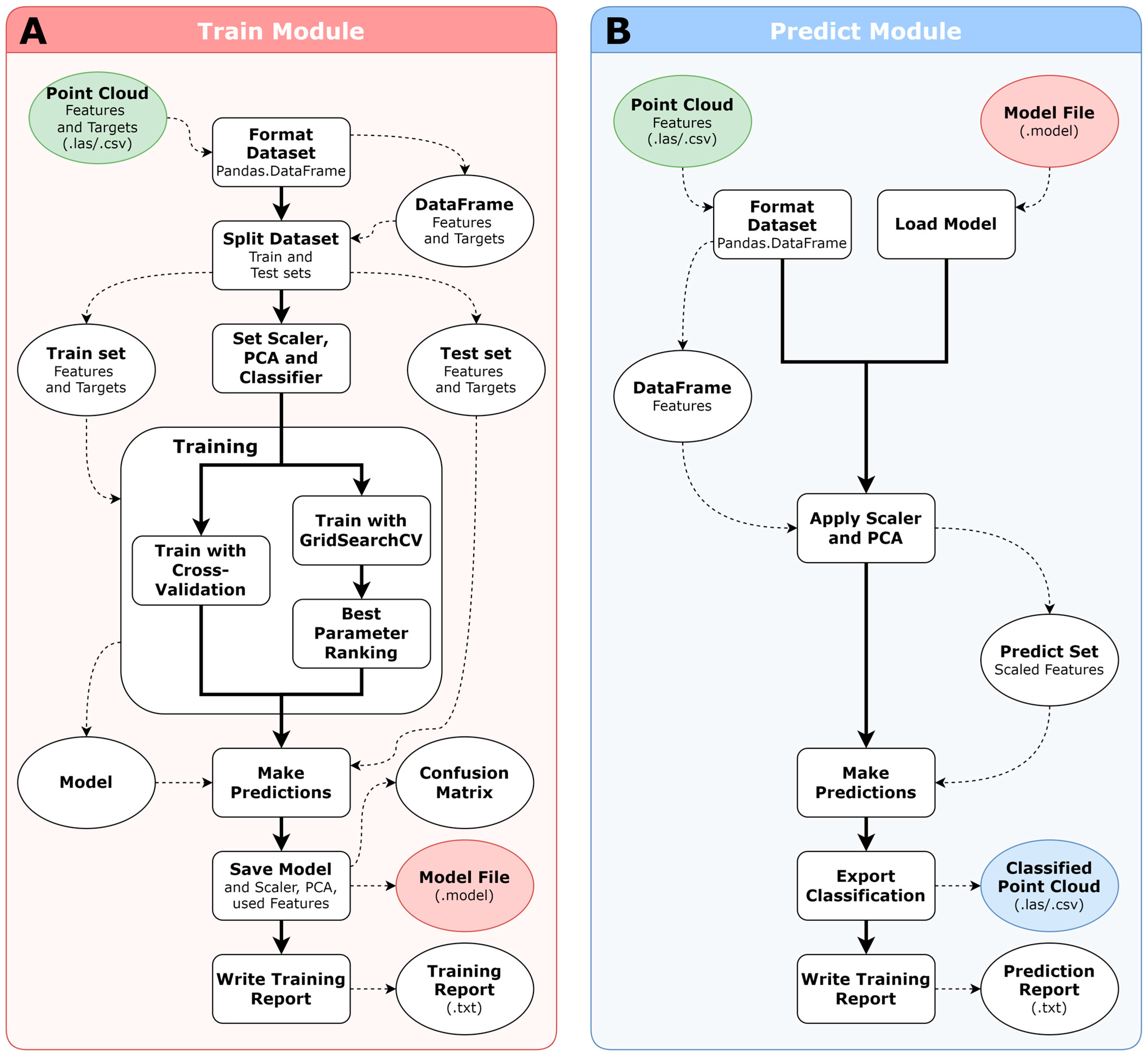
2.2.1. Training Workflow

The cLASpy_T training workflow is illustrated in Figure 2A. It begins with an input training dataset and a classifier selected from RF, GB, and MLP classifiers.

Convert 3D Point Cloud as Pandas DataFrame

To form a model, supervised ML algorithms need to be trained with a training set containing the features describing the points and the labels defining the class for each point. Its design is explained in Section 2.3. cLASpy_T loads the training dataset as a 3D point cloud from a LAS or CSV file and converts it to a Pandas DataFrame to work with the scikit-learn API. The training dataset must contain two objects: the data matrix X, the size of n samples by m features, and the vector y with one label for each sample. cLASpy_T creates two variables: data corresponding to the user-selected features from the X matrix, and target corresponding to the label vector y.

Split into Train and Test Sets

To train and test a model, the selected classifier needs a ‘train set’ and a ‘test set’ created from the training dataset. cLASpy_T uses the scikit-learn method train_test_split() to split data and target into data_train, data_test, target_train, and target_test, respectively. The data_train and target_train together form the ‘train set’, and the data_test and target_test form the ‘test set’. The size ratio between ‘train set’ and ‘test set’ can be tuned (0.8 by default).

Set the Scaler, PCA and Classifier in a Pipeline

Before training the model, cLASpy_T must apply some preprocesses to the data. The first preprocess is the scaler. All features do not share the same order of magnitude, i.e., some features are coded in 8 bits, from 0 to 255, such as RGB colors, and others in floating values, from 0 to 1, such as geometric features. For algorithms such as neural networks like MLPClassifier, the features must be calibrated to share the same scale. Several scalers are available from scikit-learn and are selectable in cLASpy_T. By default, cLASpy_T uses StandardScaler, which transforms each feature with a mean of 0 and a variance of 1. The second preprocess is PCA to reduce the number of dimensions of the ‘train set’. Considering the primary and secondary features at several scales, the total number of features can be high. With PCA, this number of dimensions can be reduced with a minimum loss of information [61]. cLASpy_T builds a pipeline with the scaler and optional PCA, then adds the classifier according to the settings of the selected algorithm. The scaler, PCA, and the classifier will be applied to the ‘train set’ in that order during the training step.

Train Model

First, cLASpy_T fits the scaler to the data_train and applies the transformation to it. If any PCA is used, the same process is applied: fit PCA to the data_train and then apply the PCA transformation to it. After the preprocesses, the selected classifier starts to train the model according to the transformed data_train and the target_train. By default, the Cross-Validation method with 5 folds is used. Cross-validation allows cLASpy_T to create multiple models with the same ‘train set’. The performance of the models can then be compared to ensure their consistency and therefore the quality of the models and the ‘train set’. Cross-validation shuffles the ‘train set’ then splits it into 5 folds. Each of the 5 models uses a different fold for its evaluation, while the other 4 folds are used for training. Thus, all the folds are used for training and evaluation purposes, and the 5 models can be compared. cLASpy_T provides the global accuracies of the 5 models to check the training. If the model results are not consistent, the ‘train set’ and the classifier parameters must be investigated to find the issue; otherwise, the training keeps the model and tests it.

Depending on the number of features, the number of points in the ‘train set’, the classifier, and its parameters, the training step can be more or less long, from one minute to several hours.

Write Training Report

To test the model, cLASpy_T retrieves the scaler and PCA transformations saved in that model and applies them to the ‘test set’. The predictions made by the model on this ‘test set’ are compared to the labels from the target_test vector. The results of this comparison are the confusion matrix and the scores of the model such as global accuracy, precision, recall, etc. The model, the scaler, the PCA transformations, and the features used are saved into a binary file (.model) that will be loaded to make further predictions with the predict module. A training report is created and includes classifier, scaler, and PCA parameters, the features used, the confusion matrix, and the scores.

2.2.2. Prediction Workflow

Load Prediction Set and Model File

Figure 2B shows the prediction workflow of cLASpy_T. The 3D point cloud of the prediction dataset is loaded by cLASpy_T from a LAS or CSV file and converted to a Pandas DataFrame. The prediction dataset needs to include the same features as those used for the training phase. The model file, previously saved at the end of the training workflow, is also loaded. The classifier is set according to the saved parameters, as are the features used, the scaler, and any PCA.

Find Features, Apply Scaler, PCA

Before going any further, the software checks that all the necessary features are present in the prediction dataset. It then applies the scaler and any PCA to the entire dataset. The prediction set is obtained with all features scaled in the same way as for model training. cLASpy_T also checks for the presence of a ‘target’ field in the dataset. If this field is present, it is discarded for predictions, but it is used at the end to create a confusion matrix for the whole dataset.

Make Predictions and Export Classification

The model makes predictions on the entire dataset. As a result, several new fields are added to the dataset:

• A ‘Prediction’ field for the classification performed by the model;
• A ‘BestProba’ field for maximum likelihood;
• A ‘ProbaClass_X’ field for each class for the likelihood per class.

The probability of a class is a floating value between 0 and 1, expressing the probability of a point belonging to that class according to the model. The maximum likelihood is the maximum likelihood value for all classes combined. If a ‘target’ field has been previously detected, a confusion matrix is created. Next, cLASpy_T exports the entire dataset in the same format as the original file (LAS or CSV), with the new fields.

Write Prediction Report

Finally, cLASpy_T writes the prediction report, similar to the training report, including the dataset, as well as the features, model, scaler, and PCA parameters, and, if applicable, the confusion matrix.

2.3. Results of Supervised Classification

2.3.1. Confusion Matrix

The performance of a trained model obtained after a classification test is expressed by several metrics, such as the confusion matrix, global accuracy, precision, and recall per class. The confusion matrix is a complete solution to expose the results of a multiclass classification. The confusion matrix below in

Table 1. Example of a confusion matrix.

		Predicted Class			Recall
		Sand	Rock	Block
Expected class	Sand	3000	150	100	92.3%
	Rock	110	1500	25	91.7%
	Block	45	160	5000	96.1%
Precision		95.1%	82.9%	97.6%	94.2%

shows the results of a fictitious concrete block classification.

The confusion matrix is based on the comparison between the class value predicted by the model for each sample of the test set and the actual expected class. The expected class values correspond to the ‘Target’ field given in the training set and are most often entered by the field expert. The columns correspond to the class predicted by the model, while the rows correspond to the expected class. For example, all samples in the ‘sand’ column are predicted as ‘sand’ by the model. Among these 3155 samples, 3000 are ‘sand’, 110 are ‘rock’, and 45 are part of the ‘block’ class. Similarly, all the samples in the ‘rock’ row belong to the ‘rock’ class. Among these 1635 true ‘rock’ samples, 1500 were correctly classified. 110 were classified as ‘sand’ and 25 as ‘block’.

Global Accuracy

Global accuracy is the ratio between the sum of all correctly predicted samples and the total number of samples. It is therefore the ratio between the diagonal of the confusion matrix and the entire table, here 94.2%:

(3000 + 1500 + 5000)/10,090

(1)

Precision

The precision of a class is the ratio between the number of correctly predicted samples and the total number of samples predicted to belong to that class. For example, in the ‘sand’ column of Table 1, the precision of the ‘sand’ class is 95.1%:

Precision = 3000/(3000 + 110 + 45)

(2)

Recall

The recall of a class is the ratio between the number of correctly predicted samples and the total number of true samples of this class. In the green line of Table 1, the recall of the ‘rock’ class is 91.7%:

Recall = 1500/(110 + 1500 + 25)

(3)

F1-Score

Per-class precision is an important value describing the success rate of the model in correctly predicting samples. However, it must always be compared to the per-class recall to verify that the vast majority of the points of this class are present. For example, having 99% precision for a class, but with 75% recall, means the model is very good, only for 3/4 of the points in that class. The remaining quarter is incorrectly classified among the other classes, which is not the purpose of automatic classification. In the confusion matrix example, the model is very good at classifying blocks, with 97.6% precision for 96.1% of the block points.

The F1-score synthesizes the complementarity between precision and recall. It is the harmonic average of precision and recall for a class:

$$F1scor{e}_{sand}=2\times {\displaystyle \frac{Precisio{n}_{sand}\times Recal{l}_{sand}}{Precisio{n}_{sand}+Recal{l}_{sand}}}$$

(4)

2.3.2. Generalization, Underfitting, and Overfitting

The main purpose of an ML model is to make the most accurate predictions possible on a dataset that has never been seen or labeled. Before achieving this result, the model must find correlations between the labels and the features contained in the training set during the training phase. At the end of the training process, cLASpy_T tests the model with similar data not used to train the model. In this study, another test is also conducted with all the data from a survey to simulate the production phase. This step allows for a more detailed analysis of the generalization with real data. To carry out this step, all the 10 million points (Mpts) per dataset are fully classified by the field expert to obtain the performance scores. Obviously, for a real production phase, the data is not pre-classified, making any calculation of performance scores impossible.

Two sets of scores are therefore available for each model: the scores after training on the test set and the scores from the production phase on the entire dataset. There are two main risks when training a model. The first is that the model is too simple to capture all aspects of the data and its variabilities, which leads to a poor model with lower scores on the test set. This is the underfitting of the model to the training data. The second risk is that the model is too complex. In this case, it perfectly models the training set. Unfortunately, while this leads to very high scores for the test set, very similar or even identical to the training set, this is not the case for the production data. The scores for the entire dataset are then significantly lower for the production phase. This is the overfitting of the model to the training data. The model is too fitted to the training set and does not allow generalization to slightly different data.

2.4. Training Set Design

Data preparation is a primary step in building a classification model from a supervised algorithm. The first step is to create a training set. As previously mentioned, to provide a good quality training set, the field expert must know the studied objects, the representation of the objects by the point cloud, and the features that best describe data points according to the classes to extract.

2.4.1. Classification Purpose

A classification, automatic or not, is defined in a specific context, for a specific purpose. Before creating a model to classify a 3D point cloud, several questions need to be answered: What are the objects to extract? What are the useless objects in the context of this study? How many different types of objects? What classes correspond to these objects? For example, consider Figure 3 showing concrete blocks on a beach near a riprap. The studied objects are the concrete blocks, and the non-studied objects are the beach and the riprap. A first binary classification with ‘block’ and ‘non-block’ classes can be tested.

2.4.2. Data Acquisition

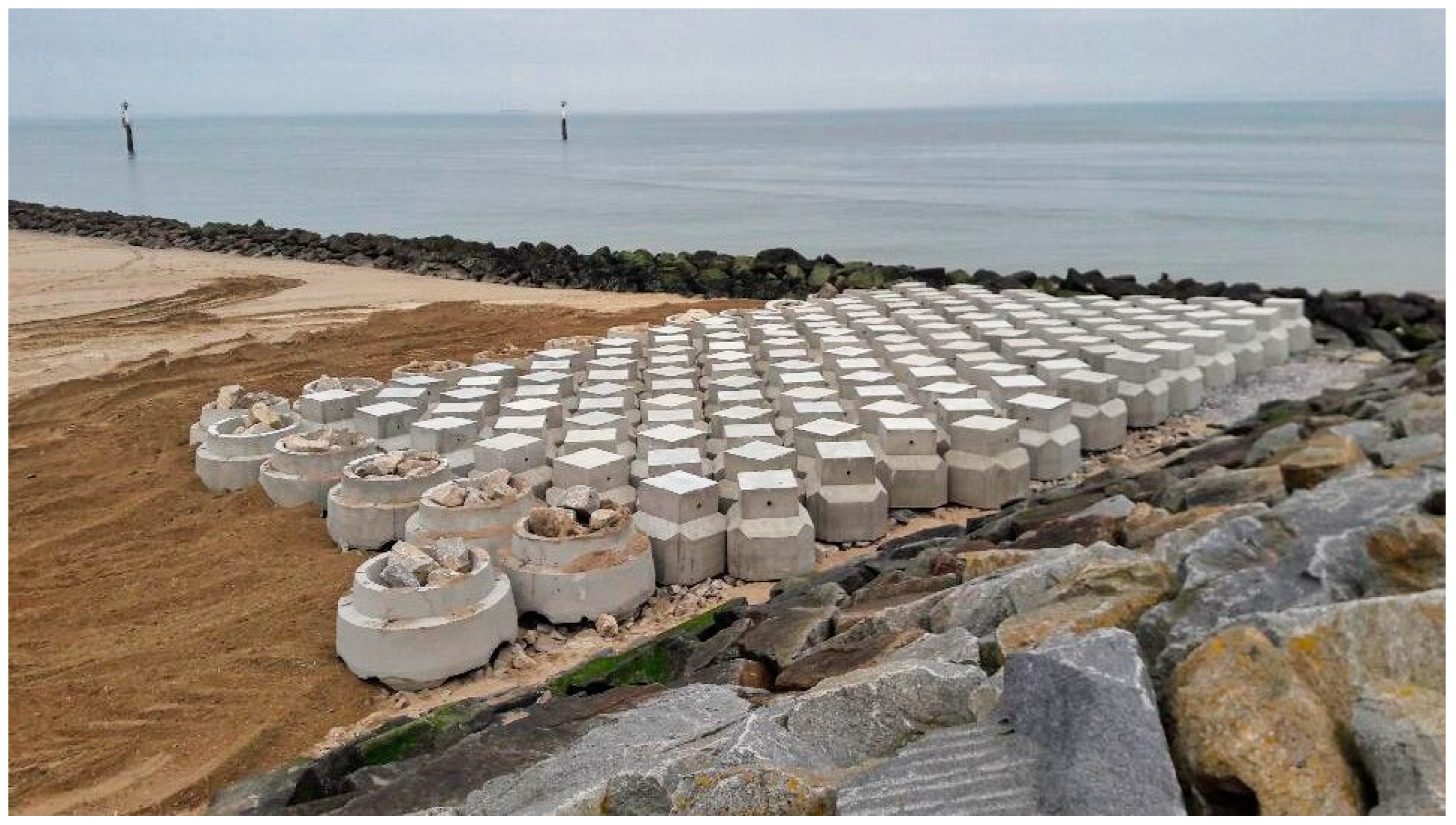
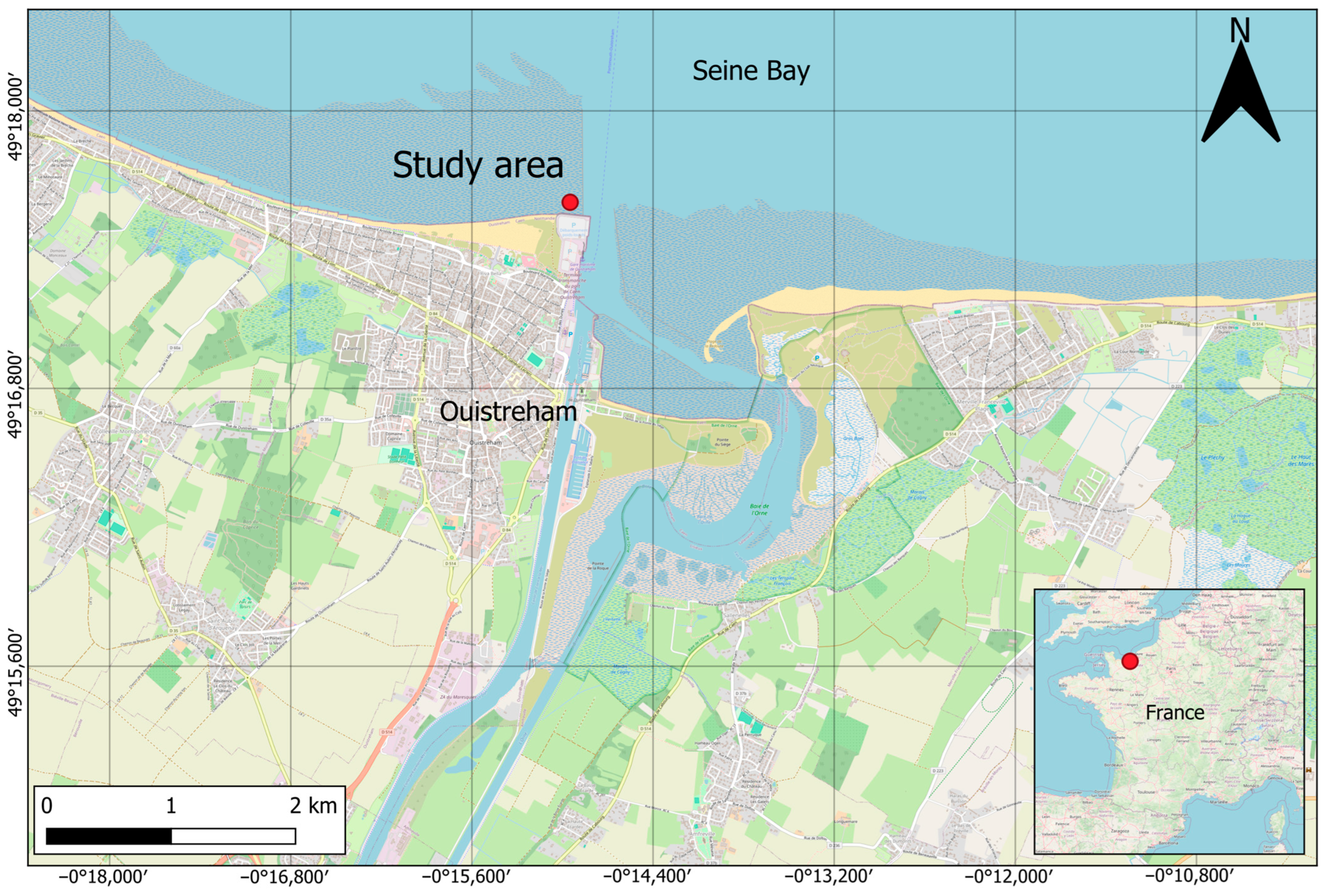
Study Site

This case study is a new kind of dike armor located in Ouistreham, a coastal city in Normandie, France (Figure 4). Its behavior through time was monitored in part by SfM photogrammetry for more than a year in the CHERLOC project. The structure has a length of 30 m and a width of 15 m and is composed of 2 different blocks: a double-cube and an Accroberm II described in [6]. We will focus on 4 of the existing surveys conducted in April, May, June, and November 2021.

Acquisition

In April 2021, 557 photos were acquired with a Canon EOS 80D camera equipped with a lens of fixed focal length of 18 mm and an aperture of F/11 to F/9. Holding a 3-m-high pole, 557 photos were taken with circle patterns at different heights, as shown on the right of Figure 5. Similarly, in May and June 2021, 566 and 646 photos were taken respectively with similar camera configurations and patterns. Lastly, in November, 722 photos were acquired in the same manner with a Sony A6000 along with a fixed focal lens of 16 mm and an aperture from F/8 to F/5.6. Processing and generation of the 3D point clouds were done by implementing SfM photogrammetry with OpenMVG [63] and OpenMVS [64] software, as described in Froideval et al., 2019 [10]. One model was obtained for each date with a few hundred million points. During the survey, 10 different targets were measured by static relative carrier base Differential GPS (DGPS) [65] with a resulting absolute georeferencing Root Mean Square Error (RMSE) of 1.8 cm for April 2021. The second date was in turn registered onto the first model with a relative RMSE of 0.7 cm. In planimetry, we used the reference system Lambert 93 and RAF09 in altimetry. The relative accuracy of the point clouds was also shown in [6] to be below 1 cm.

Table 2. Summary of photogrammetric model parameters.

Date	Camera	Focal (mm)	Aperture	Number of Photos	Number of Points (Mpts)	Referencing (cm)
						Absolute	Relative
April	Canon EOS 80D	18	F/11 to F/9	557	391	1.8	-
May		18	F/22	561	372	-	0.7
June		18	F/18 to F/16	646	471	-	0.9
November	Sony A6000	16	F/8 to F/5.6	722	431	-	0.8

summarizes the acquisition and model parameters. The resulting 3D models time series is available at https://doi.org/10.6084/m9.figshare.25908823.v1 [41]. Many formats of 3D point clouds exist, such as LAS/LAZ, PTX, XYZ, CSV, and E57. Photogrammetric software often exports result data as meshes, with PLY or OBJ formats. Currently, cLASpy_T only supports CSV and LAS formats. To import other formats in cLASpy_T, a data conversion must be done with software such as CloudCompare [66] or Meshlab [67].

2.4.3. Primary Features

Once the dataset has been obtained, depending on the acquisition method and the point cloud format, the dataset can contain useful features. These features from the original data are defined as native or primary features. They can be geometric, such as XYZ, or spectral, such as intensity or RGB. For example, in addition to XYZ coordinates, the LAS format can provide the number of returns, return number, intensity, or RGB. Figure 6 shows the RGB and Z coordinates as features of the 3D model of April 2021.

2.4.4. Data Discovery

At this stage, an initial exploration of the data should provide a better understanding of the dataset and help to roughly define the first classes. This exploration can be carried out with the help of unsupervised algorithms such as k-means clustering [68,69] or the Density-Based Spatial Clustering of Applications with Noise (DBSCAN) [70]. These algorithms group points according to their distances in feature space. These groups can then be compared with the classes being defined. A significant lack of information, and therefore of features describing the points, results in groups that are too different from the defined classes. Figure 7 shows three different segmentations of the 3D block model, with 2, 3, and 4 clusters. The only features used are the RGB data. These exploratory results show that these primary data do not appear to be sufficient for a binary “block” and “non-block” classification. Indeed, the blocks are divided into several clusters with sand or rocks, which is the opposite of the initial class definition.

It is unlikely that primary features alone will be sufficient to create a robust classification model. Depending on the accuracy of the class labels, training a model can be more or less complex. For example, it will be easier to distinguish trees and soil than to distinguish several tree species from each other. The amount of information, and therefore the number of features, will not be the same for these two examples. This initial exploration gives a good idea of what the missing features might be for a better description of the points.

2.4.5. Secondary Features

The lack of point description can be addressed by adding secondary features from computing with primary features or merging data from other sources. For example, if the classification is based on the geometry of objects, several geometric features can be computed from the primary XYZ features based on point cloud eigenvalues [71]. If the classification is based on the spectral profiles of objects, multi- or hyperspectral data from satellite, airborne, or Unmanned Aerial Vehicle (UAV) platforms can be fused with the 3D point cloud. Figure 8 shows three geometric features calculated at 0.5 m: planarity, verticality, and sphericity. Objects react differently to these features. At 0.5 m, the sandy beach is very flat, similar to the edges of Accroberms. On the other hand, the edges of these Accroberms are vertical, while the beach has very low verticality values.

Several scales of the same features are also useful to describe each point according to its close or distant neighborhood. Figure 8 also shows three different scales for verticality: 0.05 m, 0.5 m, and 1 m. At 0.05 m, the edges of Accroberms and double-cubes are easily distinguished from rocks and sand, with better resolution than at 0.5 m. The size and number of scales depend on the objects to be classified, as well as on data acquisition parameters such as point density or type of acquisition (photogrammetry, LiDAR, etc.). Defining the number of scales for each feature is part of the training set design.

Analysis of the primary and secondary features suggests that blocks and riprap are too similar and both will be grouped in the same class. So, three classes will be used for the three different objects to ensure that the concrete blocks are clearly distinguished: (1) the ‘sand’ class, (2) the ‘rock’ class for the riprap and other rocks, and (3) the ‘block’ class for the concrete blocks.

2.4.6. Class Definition

After exploring the dataset with all available features, the field expert defines the classes. Several zones are selected from the entire dataset to build the training set. These areas should describe all the defined classes as faithfully as possible, incorporating as many of their specificities as possible. For example, for the ‘block’ class in Figure 9, the training areas include double-cube blocks, Accroberms, and some double-cubes in the center. This last area will enable the model to differentiate between the flat surface of the ‘sand’ class and the flat surface of the top of the double-cubes. According to their knowledge of the studied objects and the information from features, the field expert labels each point for all selected zones. The number of points per class strongly depends on the classification complexity, the chosen algorithm, and the number of features. For easily modellable classes, 10,000 to 50,000 points per class is a good order of magnitude. Care must be taken to avoid an unbalanced distribution of classes, such as class ‘a’ being ten times class ‘b’.

All the steps of the training set design are iterative: (1) another 3D point cloud is added to the original point cloud, (2) a primary feature is discarded or added, (3) another unsupervised algorithm reveals new classes to extract, (4) a set of secondary features is removed or added and (5) some areas are added or removed from the training set. The design of the training set stops when it is representative of each class according to the field expert and the results of mini supervised learning tests.

At the end, the training set is a 3D point cloud with n points, or samples, described by m features, or dimensions. Each point has a label, or target. This 3D point cloud will be passed to cLASpy_T as input data to train the model, as shown in the training workflow (Figure 2).

2.5. Datasets

The 3D model time series provided with this study is composed of 8 files, 2 per date with one Trainset and one Dataset [41]. The first set is used to train the algorithm and is composed of 100 thousand points (kpts) per class, ‘sand’, ‘rock’ and ‘block’, for a total of 300 kpts. The Dataset, on the other hand, contains the full model with 10 Mpts. Both sets are classified manually and both contain 15 features per point: spectral features with R, G, and B along with geometric features with Volume Density, Verticality, Sphericity, and Planarity, for 3 different scales: 0.05 m, 0.5 m, and 1 m.

The geometric features were chosen considering the knowledge of the objects studied: the beach, the riprap, and the concrete blocks. The sand, for example, is expected to have very low verticality values, unlike the edges of the blocks. Scales are also very important. They have been chosen according to the size of the objects, i.e., rocks and blocks. It is expected that planarity values will vary greatly between scales of 0.05 m, 0.5 m, and 1 m, for rocks and blocks. Volume density is present to set aside the case of targets used to reference photogrammetry models.

3. Results

3.1. Algorithm Parameters and Features Selection

3.1.1. Impact of the Algorithm Parameters

The design of an automatic classification model considers a large number of elements including the training set, the number of points, the chosen algorithm along with its parameters, and the features used. Among these elements, setting the algorithm parameters is an important step to get a high-performance and optimized model. Figure 10 shows the performance of three RF models of varying degrees of complexity, depending on the algorithm’s parameter settings. The impact on prediction performance of two main parameters of RF algorithms is tested: max_depth and n_estimators. These parameters were introduced in Section 2.1.3., about the algorithms used. The three models are trained with the training set of April 2021, which includes 100 kpts of ‘train set’ used to train the models, and 100 kpts of the ‘test set’ to compute the scores of this training phase. The scores of the prediction phase are computed over the entire dataset of April with 10 Mpts. As a reminder, the scores from the prediction phase simulate the results that the models would have in production, with datasets without any label, and therefore without the possibility of calculating performance scores. All the datasets have been fully labeled in this study to report the results of the models as ‘production’ mode.

The simplest model, referred to as ‘light’, has a max_depth of 3 and n_estimators of 5. Test results for this model, corresponding to training phase performances, show a relatively low global accuracy of 82.5%, with highly variable precision and recall scores per class. The ‘rock’ class, for example, has an intermediate precision of 88.3%, and poor recall of less than 70%. As explained in the Section 2.3.2, a moderate precision for a class with only 70% of the points in that class is highly insufficient and is a sign of an underfitting model. The prediction scores show that the model is underfitted, particularly concerning the ‘rock’ class, with a very low precision of 57.6%, more than 30% lower than the test scores. The chosen parameters therefore lead to a too light classification model, which cannot correctly model all classes.

The second model, referred to as ‘fitted’, has a max_depth of 11 and n_estimators of 10. Test results for this model show a good global accuracy of 96.6%, with all precision and recall per class around this value. The global accuracy from the prediction phase is 93.5%, which is a significant improvement compared to the ‘light’ model. The precision and recall per class are consistent with this value, except for the ‘rock’ precision, at 80.4%. The settings of the two parameters lead to a more fitted model, which could be further improved regarding the ‘rock’ class.

The last model, referred to as ‘heavy’, has one hundred trees (n_estimators) and no limit for the maximum depth of each tree (max_depth). At first glance, this model appears to be an improvement over the previous one. All training phase scores are better, around 99%, as well as prediction scores. The ‘rock’ class gains almost 7% in precision, to 87.2%. However, such a high training score (99%), with lower prediction scores between 3% and 12%, should alert the model designer. An excellent model with 99% global accuracy should result in performance in the 97–99% range, with consistent scores across all classes. It seems that this model is slightly overfitted compared to the training data, which is made possible by the absence of maximum depth, which tends to create trees overfitted with respect to the training data. The problem with overfitting models is that they appear to work well in testing, but prove ineffective in production when the data is slightly different from the training data.

Setting the parameters of an algorithm is therefore essential in the design of a model. This step is time-consuming, but analyzing model performances allows identifying under, over, and well-fitted models. All ML tasks were performed with cLASpy_T on a consumer-grade computer, featuring an 8-core, 16-thread ADM Ryzen 7 1700X processor clocked at 3.8 GHz, and 32 GB of DDR4 RAM. The training time for the ‘fitted’ model is 6.8 s, compared with 20.7 s for the ‘heavy’ model. However, all training times remain low, under 30 s, because the models remain simple, with only a dozen trees per forest, 15 features, and three classes. With much larger RFs of several thousand trees, with several hundred features and more than a dozen classes, training and prediction times can last several minutes, even hours. Having an optimized model therefore minimizes training and prediction time compared to overly complex models.

3.1.2. Impact of the Features Selection

As shown in the training set design, Section 2.4, geometric and spectral features describe each point in the cloud. Not all models use each feature with the same importance. cLASpy_T lets you export the contribution of each feature, plotting their importance as given by the scikit-learn API. Figure 11 presents the list of all features with their degree of importance for the previous ‘fitted’ model. For example, Verticality at 0.5 m contributes more than 20% to the model, while Planarity at 0.05 m seems negligible, less than 1%. Creating models by selecting the most important features can lead to simpler models that are easier to generalize. What’s more, not including a set of features, such as R, G, B spectral data, for example, means that the model can also be used on data that has never had this kind of feature.

To test the importance of feature selection, the results of three models trained with different feature selections are presented in Figure 12. All these models are based on the previous ‘fitted’ model and use the dataset and training set from April 2021. The first model, and the original, uses all the features. The second model does not use color data, i.e., R, G, and B features. The last model removes the third of the least important features according to Figure 11, namely 5 features: Planarity at 0.05 m and 0.5 m, Sphericity at 0.05 m, R, and Volume Density at 0.05 m.

The results for the training phase seem to show that there are no differences between the three models. All global accuracies are around 96.5%, as are the precision and recall scores by class. Nevertheless, the scores of the prediction phase on the 10 Mpts show the impact of the features used to create a model. The second model presents a global accuracy of 90.8%, lower than the reference model based on all features, with 93.5%. The model without RGB does not model the ‘rock’ class as well, with a precision of 73.8%, well below the 80.4% of the first model. On the other hand, it seems to model the ‘block’ class quite well with a precision as good as the reference model, at 96.4%, for an intermediate recall of 91.4%. The removal of RGB has a negative impact on the performance of the second model. The third model, lacking the 5 least important features, has prediction results very close to the reference model. This feature selection does not have a negative impact on performances, which is an advantage because by reducing the number of features, it is possible to simplify the model and generalize it more easily.

For these simple RF models, the selection of features has no impact on training times, with durations less than 10 s. However, for the classification of 10 Mpts in the prediction phase, removing features significantly reduces prediction times. Thus, the model with all the features takes 108 s to classify the 10 Mpts, compared to 88 s for the model without RGB, and 81 s for the third model. The third model therefore takes 1/4 less time than the reference model to classify the 10 Mpts, with the same performances. This example demonstrates the benefit of optimizing models and training sets by selecting the best features, because for much more complex models and datasets, the time differences can be from tens of minutes to several hours.

3.2. Training, Prediction, and Model Generalization

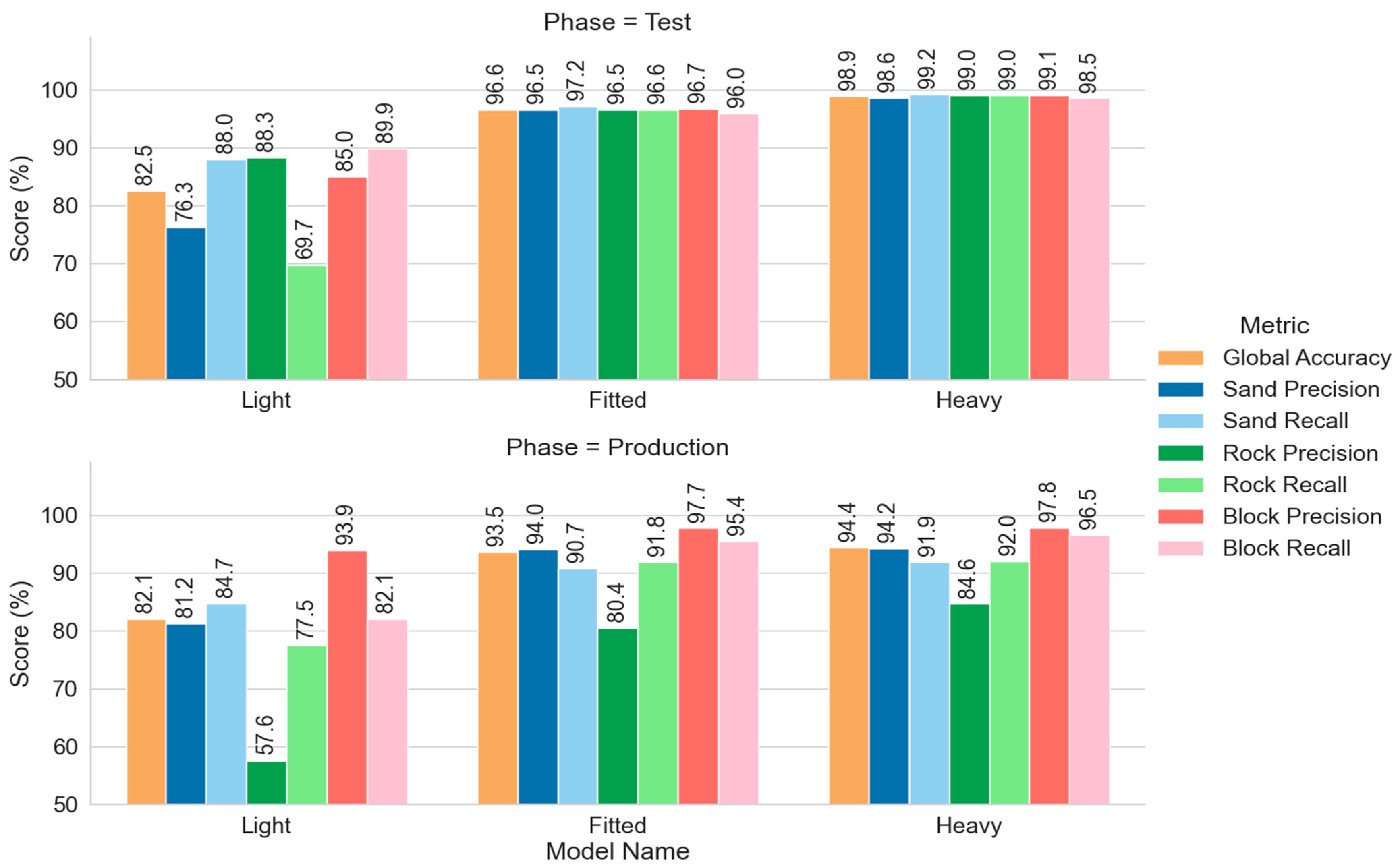
3.2.1. Simple Training and Predictions

For this section, three models were trained using the data and training sets from April 2021, similar to the previous section. These models are based on the RandomForestClassifier (RF), GradientBoostingClassifier (GB) and MLPClassifier (MLP) algorithms, respectively. The RF model is slightly more complex than the previous ‘fitted’ model to improve the modeling of the ‘rock’ class without being overfitted. The parameters of the other two models are tuned to have performances equivalent to the RF model for the April 2021 dataset, enabling comparison. The modified parameters of the three models are shown in

Table 3. Parameter settings for the three models.

Name	Scikit-Learn Algorithm	Parameter 1	Parameter 2	Parameter 3
RF	RandomForest Classifier	n_estimators 20	max_depth 12	min_samples_split 200
GB	GradientBoosting Classifier	n_estimators 50	max_depth 5	min_samples_split 200
MLP	MLP Classifer	hidden_layer_sizes [10, 5]	activation Tanh	max_iter 1000

. Their definitions are explained in Section 2.1.3. which discusses the algorithms used. All other parameters retain their default values. To compare the three types of algorithms, all features are used by the three models.

Figure 13 presents the scores of the three models for the training and prediction phases. The metrics used are global accuracy and F1-score for each of the three classes. The results on the 100 kpts test set show that all the models fit the training set very well, with scores between 96% and 97% for the three classes. During the prediction phase, all global accuracies decrease slightly by 3%, to around 93% to 94%, which is expected when switching from training mode to production mode. Furthermore, these results show that the F1-scores for the ‘block’ class are equivalent to those in the training phase, around 96%, proving that the three models modeled the ‘block’ class very well without overfitting. However, all models have a lower F1-score for the “rock” class, between 84% and 87%, which can have several related reasons: a more complex “rock” class than the other two, overly simple models, and/or a training set not sufficiently representative of this class.

For more details, an analysis of the confusion matrix provided by cLASpy_T is needed.

Table 4. Confusion matrices of the three models for the prediction phase.

		RF Predicted			RF Recall	GB Predicted			GB Recall	MLP Predicted			MLP Recall
		Sand	Rock	Block		Sand	Rock	Block		Sand	Rock	Block
Expected	Sand	2,650,977	166,696	103,761	90.7%	2,635,103	191,368	94,963	90.2%	2,685,161	159,066	77,207	91.9%
	Rock	112,400	1,484,641	19,662	91.8%	90,112	1,509,196	17,395	93.4%	97,592	1,468,478	50,633	90.8%
	Block	56,643	194,923	5,210,297	95.4%	52,846	155,879	5,253,138	96.2%	91,505	237,244	5,133,114	94.0%
Precision		94.0%	80.4%	97.7%	93.5%	94.9%	81.3%	97.9%	94.0%	93.4%	78.7%	97.6%	92.9%

presents the three confusion matrices for the three models during the prediction phase. As a first observation, the three models modeled the ‘block’ class very well, with precision and recall scores balanced around 95–97%, confirming the F1-scores. Regarding the ‘rock’ class precision, the 20% error is equally distributed between the ‘sand’ and ‘block’ classes. Therefore, there does not seem to be any preferential confusion of the ‘rock’ class with either of the other two. It is possible that complex boundary zones between classes are confusing for the models. These rock classification errors are between 300 and 400 kpts, or between 3 and 4% of the total number of points.

The MLP model has the lowest accuracy score for the “rock” class. The cLASpy_T software can export prediction results as an LAS point cloud. Figure 14 compares the predictions made by the MLP model with the expected values. The majority of points are classified well, reflected in the overall accuracy of 92.9%. Some misclassifications exist on the riprap but remain fairly easy to clarify. On the other hand, zooming in on the border of the blocks reveals points classified as “rock” instead of “sand” or “block”. In addition to predictions, cLASpy_T also exports the maximum likelihood to the LAS file, as shown at the bottom left of Figure 14. This maximum likelihood allows the user to filter predictions based on the degree of uncertainty of the model. For example, the points classified as ‘rock’ or ‘sand’ on the top of the double-cubes have low likelihoods, which allows to discard them and thus limits classification errors. Nevertheless, maximum likelihood does not counteract all misclassifications. The zoom at the bottom right in Figure 14 shows an Accroberm edge classified as ‘rock’ instead of ‘ block’, where the maximum likelihood is very high (bottom left), meaning that the model is certain it is ‘rock’.

3.2.2. Model Generalization

The main purpose of an ML model is to be used to make predictions on multiple datasets. When the results of the model remain correct over many datasets, the model is said to be generalizable. This section explores the generalization of the three models on three other datasets, compared with April 2021. Figure 15 shows the classification performances of the three models built with the April 2021 training set, on the full datasets of April, May, June, and November 2021.

The best scores are found for the April 2021 dataset. For the other datasets, all three models show significant performance losses, with global accuracies ranging from 81.9% to 88.7%. Performances for all classes are lower, from −3% to −16%, but the ‘block’ class still shows higher F1-scores than the other classes and global accuracies. The three models are therefore not generalizable to the three other datasets. Nevertheless, the higher F1-scores of the ‘block’ class show that the choice of a three-class classification —‘sand’, ‘rock’, and ‘block’ —is a good strategy. The main aim of these models is to extract blocks from 3D point clouds. This strategy seems to make it easier to model the ‘block’ class than the other two, thus improving block extraction.

Figure 16 shows the classifications performed on the April and June 2021 datasets by the GB model trained with the April training set. This model performs very well in classifying the April dataset, with high precision and recall scores, particularly for the ‘block’ class, with 97.9% precision and 96.2% recall. The ‘rock’ class still has a lower precision score of 81.3% but with a better recall score of 93.4%. Analysis of the classified point cloud reveals that the low precision corresponds to the sand around the blocks, which has been classified as ‘rock’. It is true that pebbles and small rocks can be found in these locations. This score is not so much a result of faulty modeling, but rather of manual misclassification of the dataset by the field expert. It is more a problem of defining the minimum size of a rock than an ML problem.

Observation of the June 2021 point cloud (top right of Figure 16) shows that the blocks have evolved with algae growth on Accroberms and some double-cubes. However, the GB model seems robust to Accroberms color changes since they are largely well classified, despite the algae. There are still gross errors made by the GB model, with points classified as ‘sand’ above the double cubes. The low precision of the ‘rock’ class, at 72%, seems to be caused by the pebbles and small rocks at the foot of the blocks. As for the classification in April 2021, these pebbles and small rocks are labeled ‘sand’ by the field expert but classified as ‘rock’ by the GB model. This also decreases the ‘sand’ recall.

Despite these errors, and depending on the main objective of the classification, the results of the GB model over April and June could be sufficient. Indeed, if the aim is the extraction of concrete blocks, a very large part of the extraction work is correctly carried out by the model on both datasets. Depending on the needs and within certain limits, this model can be considered generalizable.

3.3. Cross-Date Training

The previous section showed that the generalization of supervised ML models is not trivial. One possible technique to improve model generalization is to enlarge the training set by mixing several training sets from different surveys. This section presents the results obtained with three GB models trained with three different training sets: one with a single date (April), one with two dates (April-May), and one with three dates (April-May-June). All training sets count 200 kpts, with 100 kpts for training and 100 kpts for testing, and each class counts a third of the total points. The April 2021 training set uses only points from this set, i.e., around 66,666 points per class. The first half of the April-May set consists of April points, and the second half consists of May points, i.e., around 33,333 points per date and per class. The April-May-June training set comprises a third of April, a third of May, and a third of June points, i.e., around 22,222 points per date and per class.

Figure 17 shows the classification performance on the November 2021 dataset by the three GB models trained with the three different training sets. As a reminder, the November 2021 data were never used to train the models. As a first approximation, the overall accuracy of the models increases with the number of surveys added. Overall accuracy rises from 85.4% with a single date (April), to 86.8% with two dates (April-May), and reaches 89.1% with all three dates (April-May-June). However, these improvements are not linear across classes. For example, the precision of the ‘sand’ class increases from 84.9% for one date, to 92.0% for two dates, but stagnates at 92.5% for three dates. This tends to show that the information contribution of each survey is not linear. furthermore, as shown by the results for April and May 2021, the addition of surveys can also decrease some scores, such as the ‘sand’ recall, which drops from 79.2% for one date to 74.5% for two dates.

Since the purpose is to obtain a generalizable model, improving prediction performance is not the only factor to consider. Reducing performance volatility is also important. Between the April and the April-May-June training sets, performance increases while score homogeneity increases. The three-date model therefore tends toward better generalization.

Figure 18 shows the classification results for the November 2021 dataset with the models at one date, April 2021, and three dates, April, May, and June 2021. The classification of the one-date model has many gross errors, with many points of the riprap classified as ‘sand’ or ‘block’. Similarly, many points on top of double-cubes are classified as ‘sand’. Lastly, two Accroberms are almost entirely classified as ‘rock’ and concentrate the majority of ‘block’ recall defects, at 85.5% (Figure 17). Block toe misclassifications are fewer than in previous models. This is explained by the silting of pebbles and small rocks in the area between June and November 2021, thus facilitating classification.

The three-date model corrects many classification errors. A large majority of points classified as ‘sand’ on the riprap and the top of the double-cubes have been corrected. Part of the two Accroberms classified as ‘rock’ is also corrected. However, there are still points classified as ‘block’ in the riprap. The results of the three-date model can be considered correct given the number of blocks automatically extracted, namely approximately 160 out of 164 blocks.

3.4. Hierarchical Classification

It is possible to improve a model by using the results of a first classification and adding them to the training set to perform a second training and classification [31]. It is necessary that the information from the first classification, level 1, is relevant to improve the results of the level 2 classification. As shown in Figure 14, cLASpy_T records the maximum likelihoods and probabilities per class. This information is relevant because it expresses the model’s certainty in its own prediction. By combining these new features, it is possible to improve a model.

Figure 19 shows the predictions made by the GB model trained with April 2021data. Figure 19A shows that the model mistakenly classifies small areas of ‘sand’ near the blocks as ‘rock’. The expert has decided to classify small rocks as ‘sand’. This decision is also problematic in the Accroberm blocks: the GB model classifies some of the rocks as ‘sand’. It is then possible to update the training set by adding these metrics without changing the class definition. A new GB model is then trained with this updated training set. Figure 19B shows the predictions made by this new GB level 2 model. All the small rocks at the foot of the blocks are not classified as ‘sand’ but as ‘rock’. This is not consistent with the expert’s training set, but it is consistent with the data. In addition, this GB level 2 model has corrected the points classified as ‘sand’ in the Accroberms.

The information provided by the ‘BestProba’ and the class probability fields from the first classification improved the predictions made by the GB level 2 model. However, the performance of this model is no longer relevant since it is a comparison between the model results and the classes as defined by the expert. To compute the performance of this new model, a new manual classification would have to be carried out, classifying small rocks in the ‘rock’ class rather than in the ‘sand’ class.

3.5. A Classification Example with Point Cloud from ALS

This section presents the preliminary results of a classification performed with cLASpy_T on a 3D point cloud from airborne LiDAR. The data were acquired in June 2015 by a Leica ALS 60 over Ouistreham (Figure 20). This is a different spatial scale, covering the entire Orne estuary, available at https://sextant.ifremer.fr/record/93c7ba76-9a65-4144-8802-acb86343cc47 [72]. The aim of this classification is to extract five classes to analyze the evolution of the estuary over several years. These five classes are: ‘water’, ‘road, parking’, ‘buildings, trees’, ‘grass, schorre’, and ‘sand, mud’. The training set consists of the two red rectangles in Figure 20B. The training of an RF model was performed with 100 kpts per class from the training set of 1 Mpts, available at https://doi.org/10.6084/m9.figshare.26346709.v1 [73]. The spectral features are RGB at 1 m and Intensity at 0, 2, 5, 10, and 25 m. Geometric features are Linearity, Number of returns, Omnivariance, Planarity, Roughness, Sphericity, Surface variation, and Verticality at scales of 2, 5, 10, and 25 m. The RF model is trained with the train module of cLASpy_T. This model is simple, with the following parameters: n_estimators = 100, max_depth = 20, and min_samples_split = 500. The other parameters are set to their default values. The RF model is used with the predict module of cLASpy_T on a 18 Mpts point cloud [73]. Prediction performance is good, with global accuracy of 87.2%, mostly due to the 96.7% accuracy of the ‘sand, mud’ class (Figure 20). The precision of the ‘water’ class is low, at around 74%, but its recall is high, at 93.6%. This is due to the large number of areas classified as ‘water’ on the beach (Figure 20B,C). These errors are mainly due to a difference between the modeling and the field expert’s interpretation. The ‘road, parking’ and ‘buildings, trees’ classes have average precision and recall, between 85 and 87%. The model shows poor performance for the ‘grass, schorre’ class, with less than 76% recall and only 69.5% precision. Nevertheless, the model’s predictions for this class also appear to be more consistent with the data than the field expert’s classification. These preliminary results are very promising, given the restricted areas used for training.

4. Discussion

4.1. A Model Design Example

The purpose of this work is not to create the best model for point cloud classification but to present a use case of classification model design for remote sensing data in a coastal environment. Section 3.1.1 demonstrates the importance of adjusting the algorithm parameters to avoid the risk of underfitting the data with a simple model or overfitting with a model that is too complex. This is a long and tedious task, requiring a great deal of trial and error. Users should bear in mind the ultimate objective of an ML model: to predict the values of new data, not the values of already known data. Section 3.1.2 presents the impact of features on model performance. The selection of features can be based on their nature, either spectral or geometric, or on their scales. The method presented in this study uses the contribution of each feature plotted by cLASpy_T via the scikit-learn API. It is up to the user to define a threshold according to the complexity of the classes and the expected performance. It is also possible to select features and scales hierarchically, as shown in Teruggi et al., 2020 [31]. Feature selection can also reduce the number of dimensions so that simpler, more generalizable models can be used. Other methods exist for reducing the number of feature space dimensions, such as PCA, which can be used in cLASpy_T [74]. Section 3.2 shows the results of training three models based on the three types of algorithms available in cLASpy_T: RandomForestClassifier, GradientBoostingClassifier, and MLPClassifier. The benefit of implementing different types of algorithms in the model design is to analyze the consistency of the results of the different algorithms, depending on their parameters and the features/scales used.

Generalizing models can be a difficult task considering the classes and desired performance. Section 3.2.2 shows that models trained with one SfM survey of a dike can be completely unsuitable for other SfM surveys of the same dike. On the other hand, other models can present satisfactory results for the extraction of concrete blocks, such as the GB model. This distinction is very dependent on performance expectations and the final analysis by the field expert. A method to improve generalization is presented in Section 3.3. Its principle is to increase the variance in the training set by adding points from other training sets for the same type of object, data, and acquisition. This method could be applied to an entire coastal community by sharing training datasets with labeled point clouds via a platform. Another method could be to share models created by the community via a platform and create a catalog of machine learning models for the coastal community. All these models could thus be used, adapted, and improved.

4.2. Classification for Point Clouds from Other Sensors

We demonstrated the use of cLASpy_T for point clouds derived from SfM photogrammetry, but a similar approach could be adopted for point clouds from ALS or Terrestrial Laser Scanning (TLS) since it is based on general-purpose algorithms and on point-by-point geometric and spectral description. As shown in Section 3.5, cLASpy_T supports point clouds from airborne LiDAR. The results in Figure 20 demonstrate that the algorithms used by cLASpy_T, RF, GB, and MLP, are versatile.

Classification performance could be affected by point density for the geometry features, spectral information availability, acquisition geometry, and scan pattern. For instance, ALS and TLS do not always include RGB information but have some reflectance channels that could serve as different spectral features. In addition, cLASpy_T can be applied to a point cloud derived from a combination of two sensors such as ALS and TLS. Performance could depend on the resulting point density and spectral information available.

4.3. Manual vs. ML Classification

In this study, we described how to use cLASpy_T to assist the development of ML training models. We now consider the energy spent adopting this approach compared to simple manual classification with respect to time consumption, accuracy, and accessibility. With regard to duration, if we take one of the CHERLOC datasets as an example, containing roughly 400 million points and considering only three classes (sand, rock, and block), we could estimate the time spent on manual classification to be a few hours. With cLASpy_T, data preparation with a proper set of features would also take a few hours, and then the training and prediction would take only a few minutes on a regular desktop computer. A final step of manually checking errors would also be necessary and would require less than an hour or so. Overall, the time spent adopting either approach might be about the same for this case. If we now take a second example where we have datasets twice as big, or two similar datasets, then cLASpy_T would take about the same time as the first example, whereas manual classification would take twice as much time. As far as accuracy is concerned, manual classification could be better than ML, which requires a thorough manual check in any case. However, a prediction made with cLASpy_T classifies the dataset point by point, which is almost impossible for a human operator. Another key aspect is the subjectivity of manual classification. Indeed, object class interpretation sometimes depends on the operator. Using ML helps bring an objective and systematic method. Lastly, manual classification is more accessible as it is sufficient to know how to use a few simple tools in any point cloud software. As described in this paper, using cLASpy_T requires more knowledge and practice to design ML models and avoid traps such as overfitting. Nowadays, point cloud ML classification still needs to be democratized, which is the main goal of this work.

4.4. Using cLASpy_T or Not for ML Model Design

Overall, cLASpy_T assists the user in the design of ML models to classify 3D point clouds for their own applications. It enables ML algorithms to be used directly with point clouds in LAS and CSV formats. In its current state, the software already allows the user to access three different algorithms from the scikit-learn API and to set their parameters. Once the parameters are set and the features selected, the training and prediction workflows are automatic from data loading to result export, reducing the risk of error. There is no need for coding, testing, or debugging compared to using the scikit-learn API directly. Similarly, cLASpy_T saves the models with the scaler, PCA, and features used in a single file, thus reducing potential errors when using the models.

cLASpy_T offers two types of interfaces, leaving the user free to choose the one most suited to their needs. The CLI is simple, stable, and commands can be sent in batches, making it ideal for production phases or serial training. The GUI is more user-friendly, allowing easy selection of features or setting algorithm parameters. Moreover, the GUI allows the user to create configuration files to save settings for a training or prediction task, making it possible to create numerous tasks from variations of the same original task. This helps users design models by performing multiple cases easily to test the different parameters that need to be fine-tuned. The combination of these configuration files and the batch commands sent via the CLI means that a large number of training or prediction tasks can be carried out rapidly. This study, for example, required the creation of over 50 models and the execution of over a hundred predictions. With times on the order of a few minutes, cLASpy_T made it possible to achieve this in 15 to 20 h, producing around 200 GB of data from the four SfM surveys, i.e., 6 GB. cLASpy_T simplifies the creation of ML models, but is not intended to hide their construction or create black boxes. This is why cLASpy_T is based on a well-known and well-documented open-source library.

Nonetheless, cLASpy_T is still under development, and further improvements will be made. For instance, to increase performance, parallel GPU computing should be implemented by using a different ML library such as PyTorch [38] or TensorFlow [48]. Another enhancement that could be proposed is the support of other 3D formats such as PLY, E57, or OBJ. cLASpy_T is based on general-purpose classifiers which can be used with a wide variety of data. Support for other data types will be added, such as 2D rasters in GEOTIFF format. Using cLASpy_T for point cloud classification will never be 100% accurate because of the statistical nature of ML as well as the different possible choices of training set, features, or algorithm. A human point of view from a field expert of the particular location and of the desired classes will always be necessary to assess the quality of the final classification.

We showed the importance of the different trained models and now encourage the community to discuss the models and exchange model files trained on particular cases. Since the code of cLASpy_T is available on GitHub: https://github.com/TrickyPells/cLASpy_T [27], it includes a discussions section where users can talk about their models. This could eventually provide the basis for a catalog of 3D point cloud classification models.

5. Conclusions

The aim of this study was to present cLASpy_T, a new tool for the automatic classification of 3D point clouds. Using supervised ML algorithms to classify small point clouds with objects easily extractable with one or two features is not necessarily a good solution. However, for large point clouds with complex objects to extract, or for time series, using ML can save a lot of time.

Spending time on the production of high-quality training sets is also a factor in deciding whether or not to use ML. As shown in this study, the quality of training sets is critical in obtaining models that can be generalized. cLASpy_T has been created to support field experts, particularly coastal experts, in discovering ML with their own data. Of course, cLASpy_T and the algorithms used are not perfect, and a thorough analysis of the final classifications is always necessary.

The hope of cLASpy_T is to make the creation of ML models accessible to experts in the field and in environmental remote sensing data. Their knowledge will differentiate between a correct classification model and an incorrect one. Adding meaning to remote sensing data through automatic classification is a significant asset for the analysis of coastal, forest, mountain, or urban environments. cLASpy_T aims to help these communities create their own AI models and become familiar with the many existing ML tools.

References

1. Xie, Y.; Tian, J.; Zhu, X.X. Linking Points With Labels in 3D: A Review of Point Cloud Semantic Segmentation. IEEE Geosci. Remote Sens. Mag. 2020, 8, 38–59. [Google Scholar] [CrossRef]
2. Sturdivant, E.; Lentz, E.; Thieler, E.R.; Farris, A.; Weber, K.; Remsen, D.; Miner, S.; Henderson, R. UAS-SfM for Coastal Research: Geomorphic Feature Extraction and Land Cover Classification from High-Resolution Elevation and Optical Imagery. Remote Sens. 2017, 9, 1020. [Google Scholar] [CrossRef]
3. Le Mauff, B.; Juigner, M.; Ba, A.; Robin, M.; Launeau, P.; Fattal, P. Coastal Monitoring Solutions of the Geomorphological Response of Beach-Dune Systems Using Multi-Temporal LiDAR Datasets (Vendé e Coast, France). Geomorphology 2018, 304, 121–140. [Google Scholar] [CrossRef]
4. Pellerin Le Bas, X.; Levoy, F.; Robin, N.; Anthony, E.J. The Formation and Morphodynamics of Complex Multi-hooked Spits and the Contribution of Swash Bars. Earth Surf. Process. Landf. 2021, 47, esp.5236. [Google Scholar] [CrossRef]
5. Bakula, K.; Salach, A.; Zelaya Wziatek, D.; Ostrowski, W.; Gorski, K.; Kurczynski, Z. Evaluation of the Accuracy of Lidar Data Acquired Using a UAS for Levee Monitoring: Preliminary Results. Int. J. Remote Sens. 2017, 38, 2921–2937. [Google Scholar] [CrossRef]
6. Froideval, L.; Conessa, C.; Pellerin Le Bas, X.; Benoit, L.; Mouazé, D. Efficient Dike Monitoring Using Terrestrial SfM Photogrammetry. ISPRS Ann. Photogramm. Remote Sens. Spatial Inf. Sci. 2022, 2, 359–366. [Google Scholar] [CrossRef]
7. Gonçalves, D.; Gonçalves, G.; Pérez-Alvavez, J.A.; Andriolo, U. On the 3D Reconstruction of Coastal Structures by Unmanned Aerial Systems with Onboard Global Navigation Satellite System and Real-Time Kinematics and Terrestrial Laser Scanning. Remote Sens. 2022, 14, 1485. [Google Scholar] [CrossRef]
8. Westoby, M.J.; Brasington, J.; Glasser, N.F.; Hambrey, M.J.; Reynolds, J.M. ‘Structure-from-Motion’ Photogrammetry: A Low-Cost, Effective Tool for Geoscience Applications. Geomorphology 2012, 179, 300–314. [Google Scholar] [CrossRef]
9. Medjkane, M.; Maquaire, O.; Costa, S.; Roulland, T.; Letortu, P.; Fauchard, C.; Antoine, R.; Davidson, R. High-Resolution Monitoring of Complex Coastal Morphology Changes: Cross-Efficiency of SfM and TLS-Based Survey (Vaches-Noires Cliffs, Normandy, France). Landslides 2018, 15, 1097–1108. [Google Scholar] [CrossRef]
10. Froideval, L.; Pedoja, K.; Garestier, F.; Moulon, P.; Conessa, C.; Pellerin Le Bas, X.; Traoré, K.; Benoit, L. A Low-cost Open-source Workflow to Generate Georeferenced 3D SfM Photogrammetric Models of Rocky Outcrops. Photogram Rec. 2019, 34, phor.12297. [Google Scholar] [CrossRef]
11. Wang, L.; Zhang, Y.; Wang, J. Map-Based Localization Method for Autonomous Vehicles Using 3D-LIDAR. IFAC-Pap. OnLine 2017, 50, 276–281. [Google Scholar] [CrossRef]
12. Hu, Q.; Yang, B.; Xie, L.; Rosa, S.; Guo, Y.; Wang, Z.; Trigoni, N.; Markham, A. RandLA-Net: Efficient Semantic Segmentation of Large-Scale Point Clouds. In Proceedings of the IEEE/CVF Conference on Computer Vision and Pattern Recognition (CVPR), Seattle, WA, USA, 13–19 June 2020. [Google Scholar]
13. Jazayeri, I.; Rajabifard, A.; Kalantari, M. A Geometric and Semantic Evaluation of 3D Data Sourcing Methods for Land and Property Information. Land Use Policy 2014, 36, 219–230. [Google Scholar] [CrossRef]
14. Li, J.; Liu, J.; Huang, Q. PointDMM: A Deep-Learning-Based Semantic Segmentation Method for Point Clouds in Complex Forest Environments. Forests 2023, 14, 2276. [Google Scholar] [CrossRef]
15. Mukhandi, H.; Ferreira, J.F.; Peixoto, P. SyS3DS: Systematic Sampling of Large-Scale LiDAR Point Clouds for Semantic Segmentation in Forestry Robotics. Sensors 2024, 24, 823. [Google Scholar] [CrossRef] [PubMed]
16. Pellerin Le Bas, X. cLASpy_T v0.3. Available online: https://github.com/TrickyPells/cLASpy_T (accessed on 4 August 2024).
17. Rabbani, T.; Heuvel, F.A.; Vosselman, G. Segmentation of Point Clouds Using Smoothness Constraint. Int. Arch. Photogramm. Remote Sens. Spat. Inf. Sci. 2006, 36, 248–253. [Google Scholar]
18. Bhanu, B.; Lee, S.; Ho, C.-C.; Henderson, T.C. Range Data Processing: Representation of Surfaces by Edges. In Proceedings of the Eighth International Conference on Pattern Recognition, Paris, France, 27–31 October 1986; p. 15. [Google Scholar]
19. Vo, A.-V.; Truong-Hong, L.; Laefer, D.F.; Bertolotto, M. Octree-Based Region Growing for Point Cloud Segmentation. ISPRS J. Photogramm. Remote Sens. 2015, 104, 88–100. [Google Scholar] [CrossRef]
20. Xu, L.; Oja, E.; Kultanen, P. A New Curve Detection Method: Randomized Hough Transform (RHT). Pattern Recognit. Lett. 1990, 11, 331–338. [Google Scholar] [CrossRef]
21. Fischler, M.A.; Bolles, R.C. Random Sample Consensus: A Paradigm for Model Fitting with Applications to Image Analysis and Automated Cartography. Commun. ACM 1981, 24, 381–395. [Google Scholar] [CrossRef]
22. Filin, S. Surface Clustering from Airborne Laser Scanning Data. Int. Arch. Photogramm. Remote Sens. Spat. Inf. Sci. 2002, 34, 119–124. [Google Scholar]
23. Xu, Y.; Yao, W.; Tuttas, S.; Hoegner, L.; Stilla, U. Unsupervised Segmentation of Point Clouds From Buildings Using Hierarchical Clustering Based on Gestalt Principles. IEEE J. Sel. Top. Appl. Earth Obs. Remote Sens. 2018, 11, 4270–4286. [Google Scholar] [CrossRef]
24. Weinmann, M.; Schmidt, A.; Mallet, C.; Hinz, S.; Rottensteiner, F.; Jutzi, B. Contextual Classification of Point Cloud Data by Exploiting Individual 3d Neigbourhoods. ISPRS Ann. Photogramm. Remote Sens. Spatial Inf. Sci. 2015, II-3/W4, 271–278. [Google Scholar] [CrossRef]
25. Su, H.; Maji, S.; Kalogerakis, E.; Learned-Miller, E. Multi-View Convolutional Neural Networks for 3D Shape Recognition. In Proceedings of the IEEE International Conference on Computer Vision (ICCV), Santiago, Chile, 7–13 December 2015. [Google Scholar]
26. Maturana, D.; Scherer, S. VoxNet: A 3D Convolutional Neural Network for Real-Time Object Recognition. In Proceedings of the 2015 IEEE/RSJ International Conference on Intelligent Robots and Systems (IROS), Hamburg, Germany, 28 September–3 October 2015; pp. 922–928. [Google Scholar]
27. Zhang, J.; Lin, X.; Ning, X. SVM-Based Classification of Segmented Airborne LiDAR Point Clouds in Urban Areas. Remote Sens. 2013, 5, 3749–3775. [Google Scholar] [CrossRef]
28. Vosselman, G.; Coenen, M.; Rottensteiner, F. Contextual Segment-Based Classification of Airborne Laser Scanner Data. ISPRS J. Photogramm. Remote Sens. 2017, 128, 354–371. [Google Scholar] [CrossRef]
29. Müller, A.C.; Guido, S. Introduction to Machine Learning with Python: A Guide for Data Scientists, 1st ed.; O’Reilly: Beijing, China; Boston, MA, USA; Farnham, UK; Sebastopol, CA, USA; Tokyo, Japan, 2016; ISBN 978-1-4493-6941-5. [Google Scholar]
30. Qian, G.; Hamdi, A.; Zhang, X.; Ghanem, B. Pix4Point: Image Pretrained Standard Transformers for 3D Point Cloud Understanding. arXiv 2022, arXiv:2208.12259. [Google Scholar]
31. Teruggi, S.; Grilli, E.; Russo, M.; Fassi, F.; Remondino, F. A Hierarchical Machine Learning Approach for Multi-Level and Multi-Resolution 3D Point Cloud Classification. Remote Sens. 2020, 12, 2598. [Google Scholar] [CrossRef]
32. Axelsson, P. Processing of Laser Scanner Data—Algorithms and Applications. ISPRS J. Photogramm. Remote Sens. 1999, 54, 138–147. [Google Scholar] [CrossRef]
33. Axelsson, P. DEM Generation from Laser Scanner Data Using Adaptive Tin Models. Int. Arch. Photogramm. Remote Sens. 2000, 33 (Part B3), 85–92. [Google Scholar]
34. Arttu Soininen Terrasolid TerraScan. Available online: https://terrasolid.com (accessed on 4 August 2024).
35. Sithole, G.; Vosselman, G. Experimental Comparison of Filter Algorithms for Bare-Earth Extraction from Airborne Laser Scanning Point Clouds. ISPRS J. Photogramm. Remote Sens. 2004, 59, 85–101. [Google Scholar] [CrossRef]
36. Brodu, N.; Lague, D. 3D Terrestrial Lidar Data Classification of Complex Natural Scenes Using a Multi-Scale Dimensionality Criterion: Applications in Geomorphology. ISPRS J. Photogramm. Remote Sens. 2012, 68, 121–134. [Google Scholar] [CrossRef]
37. Gaydon, C. Myria3D: Deep Learning for the Semantic Segmentation of Aerial Lidar Point Clouds; IGN (French Mapping Agency): Paris, France, 2022. [Google Scholar]
38. Falcon, W. The PyTorch Lightning Team PyTorch Lightning 2019. Available online: https://github.com/Lightning-AI/pytorch-lightning (accessed on 4 August 2024).
39. Pedregosa, F.; Varoquaux, G.; Gramfort, A.; Michel, V.; Thirion, B.; Grisel, O.; Blondel, M.; Prettenhofer, P.; Weiss, R.; Dubourg, V.; et al. Scikit-Learn: Machine Learning in Python. J. Mach. Learn. Res. 2011, 12, 2825–2830. [Google Scholar]
40. Buitinck, L.; Louppe, G.; Blondel, M.; Pedregosa, F.; Mueller, A.; Grisel, O.; Niculae, V.; Prettenhofer, P.; Gramfort, A.; Grobler, J.; et al. API Design for Machine Learning Software: Experiences from the Scikit-Learn Project. In Proceedings of the ECML PKDD Workshop: Languages for Data Mining and Machine Learning, Prague, The Czech Republic, 23-27 September 2013; pp. 108–122. [Google Scholar]
41. Froideval, L.; Conessa, C.; Laurent, B. 3D Model Time Series of a Coastal Dike in Ouistreham, France 2024, 3258744154 Bytes. Available online: https://doi.org/10.6084/m9.figshare.25908823.v1 (accessed on 4 August 2024).
42. Hackel, T.; Savinov, N.; Ladicky, L.; Wegner, J.D.; Schindler, K.; Pollefeys, M. Semantic3D.Net: A New Large-Scale Point Cloud Classification Benchmark. arXiv 2017, arXiv:1704.03847. [Google Scholar] [CrossRef]
43. Hu, Q.; Yang, B.; Khalid, S.; Xiao, W.; Trigoni, N.; Markham, A. Towards Semantic Segmentation of Urban-Scale 3D Point Clouds: A Dataset, Benchmarks and Challenges. In Proceedings of the IEEE/CVF Conference on Computer Vision and Pattern Recognition, Nashville, TN, USA, 20–25 June 2021. [Google Scholar]
44. Gaydon, C.; Daab, M.; Roche, F. FRACTAL: An Ultra-Large-Scale Aerial Lidar Dataset for 3D Semantic Segmentation of Diverse Landscapes. arXiv 2024, arXiv:2405.04634. [Google Scholar]
45. Gaydon, C.; Roche, F. PureForest: A Large-Scale Aerial Lidar and Aerial Imagery Dataset for Tree Species Classification in Monospecific Forests. arXiv 2024, arXiv:2404.12064. [Google Scholar]
46. Artelnics OpenNN. Available online: https://github.com/Artelnics/OpenNN (accessed on 4 August 2024).
47. Sonnenburg, S.; Raetsch, G.; Henschel, S.; Widmer, C.; Behr, J.; Zien, A.; de Bona, F.; Binder, A.; Gehl, C.; Franc, V. The Shogun Machine Learning Toolbox. J. Mach. Learn. Res. 2010, 11, 1799–1802. [Google Scholar]
48. Abadi, M.; Agarwal, A.; Barham, P.; Brevdo, E.; Chen, Z.; Citro, C.; Corrado, G.S.; Davis, A.; Dean, J.; Devin, M.; et al. TensorFlow: Large-Scale Machine Learning on Heterogeneous Systems. arXiv 2015, arXiv:1603.04467. [Google Scholar]
49. Bergstra, J.; Bengio, Y. Random Search for Hyper-Parameter Optimization. J. Mach. Learn. Res. 2012, 13, 281–305. [Google Scholar]
50. Allen, D.M. The Relationship Between Variable Selection and Data Agumentation and a Method for Prediction. Technometrics 1974, 16, 125–127. [Google Scholar] [CrossRef]
51. Stone, M. Cross-Validatory Choice and Assessment of Statistical Predictions. J. R. Stat. Soc. Ser. B Stat. Methodol. 1974, 36, 111–133. [Google Scholar] [CrossRef]
52. Breiman, L. Arcing Classifiers. Ann. Stat. 1998, 26, 801–824. [Google Scholar]
53. Breiman, L. Random Forests. Mach. Learn. 2001, 45, 5–32. [Google Scholar] [CrossRef]
54. Friedman, J.H. Greedy Function Approximation: A Gradient Boosting Machine. Ann. Stat. 2001, 29, 1189–1232. [Google Scholar] [CrossRef]
55. Friedman, J.H. Stochastic Gradient Boosting. Comput. Stat. Data Anal. 2002, 38, 367–378. [Google Scholar] [CrossRef]
56. Hastie, T.; Tibshirani, R.; Friedman, J.H. The Elements of Statistical Learning: Data Mining, Inference, and Prediction, 2nd ed.; Springer Series in Statistics; Springer: New York, NY, USA, 2009; ISBN 978-0-387-84857-0. [Google Scholar]
57. Hinton, G.E. Connectionist Learning Procedures. Artif. Intell. 1989, 40, 185–234. [Google Scholar] [CrossRef]
58. Glorot, X.; Bengio, Y. Understanding the Difficulty of Training Deep Feedforward Neural Networks. In Proceedings of the Thirteenth International Conference on Artificial Intelligence and Statistics, Chia Laguna Resort, Sardinia, Italy, 13 May 2010; Teh, Y.W., Titterington, M., Eds.; Volume 9, pp. 249–256. [Google Scholar]
59. Kingma, D.P.; Ba, J. Adam: A Method for Stochastic Optimization. arXiv 2014, arXiv:1412.6980. [Google Scholar] [CrossRef]
60. He, K.; Zhang, X.; Ren, S.; Sun, J. Delving Deep into Rectifiers: Surpassing Human-Level Performance on ImageNet Classification. In Proceedings of the International Conference on Computer Vision, Las Condes, Chile, 11–18 December 2015. [Google Scholar] [CrossRef]
61. Jolliffe, I.T. Principal Component Analysis, 2nd ed.; Springer Series in Statistics; Springer: New York, NY, USA, 2002; ISBN 978-0-387-95442-4. [Google Scholar]
62. QGIS Development Team. QGIS 3.34 Geographic Information System; QGIS Development Team: Zurich, Switzerland, 2024. [Google Scholar]
63. Moulon, P.; Monasse, P.; Perrot, R.; Marlet, R. OpenMVG: Open Multiple View Geometry. In Reproducible Research in Pattern Recognition: First International Workshop, Proceedings of the Reproducible Research in Pattern Recognition, Cancún, Mexico, 4 December 2016; Kerautret, B., Colom, M., Monasse, P., Eds.; Springer International Publishing: Berlin/Heidelberg, Germany, 2017; pp. 60–74. [Google Scholar]
64. Cernea, D. OpenMVS v2.3.0: Multi-View Stereo Reconstruction Library. Available online: https://github.com/cdcseacave/openMVS (accessed on 4 August 2024).
65. Bisnath, S.; Uijt de Haag, M.; Diggle, D.W.; Hegarty, C.; Milbert, D.; Walter, T. Differential GNSS and Precise Point Positioning. In Understanding GPS/GNSS: Principles and Applications; GNSS Technology and Applications Series; Artech House: Boston, MA, USA; London, UK, 2017; pp. 709–788. ISBN 978-1-63081-058-0. [Google Scholar]
66. Girardeau-Montaut, D. CloudCompare (Version 2.13.1) [GPL Software]; 2024. Available online: https://www.danielgm.net/cc/ (accessed on 4 August 2024).
67. Cignoni, P.; Callieri, M.; Corsini, M.; Dellepiane, M.; Ganovelli, F.; Ranzuglia, G. MeshLab: An Open-Source Mesh Processing Tool. In Proceedings of the European Interdisciplinary Cybersecurity Conference, Edinburgh, UK, 25–28 May 2008. [Google Scholar]
68. Lloyd, S. Least Squares Quantization in PCM. IEEE Trans. Inform. Theory 1982, 28, 129–137. [Google Scholar] [CrossRef]
69. MacQueen, J. Some Methods for Classification and Analysis of Multivariate Observations. In Proceedings of the Fifth Berkeley Symposium on Mathematical Statistics and Probability, Oakland, CA, USA, 1 January 1967; Volume 1, pp. 281–297. [Google Scholar]
70. Ester, M.; Kriegel, H.-P.; Sander, J.; Xu, X. A Density-Based Algorithm for Discovering Clusters in Large Spatial Databases with Noise. In Proceedings of the KDD, Portland, OR, USA, 2–4 August 1996; Volume 96, pp. 226–231. [Google Scholar]
71. Hackel, T.; Wegner, J.D.; Schindler, K. Contour Detection in Unstructured 3D Point Clouds. In Proceedings of the 2016 IEEE Conference on Computer Vision and Pattern Recognition (CVPR), Las Vegas, NV, USA, 27–30 June 2016; pp. 1610–1618. [Google Scholar]
72. Froideval, L.; Monfort, O.; Benoit, L.; Bonte, Y. Mesure Topographique par LiDAR Aéroporté et Modèle Numérique Terrain de l’estuaire de l’Orne du 03/06/2015. Available online: https://sextant.ifremer.fr/record/93c7ba76-9a65-4144-8802-acb86343cc47 (accessed on 4 August 2024).
73. Froideval, L.; Pellerin Le Bas, X.; Conessa, C.; Laurent, B. ALS Orne Estuary ML Labeled Data 2024, 6597898321 Bytes. Available online: https://doi.org/10.6084/m9.figshare.26346709.v1 (accessed on 4 August 2024).
74. Tipping, M.E.; Bishop, C.M. Mixtures of Probabilistic Principal Component Analyzers. Neural Comput. 1999, 11, 443–482. [Google Scholar] [CrossRef]
Figure 1. Supervised classification workflow.
Remotesensing 16 02891 g001
Figure 2. cLASpy_T workflows for training (A) and prediction modules (B).
Remotesensing 16 02891 g002
Figure 3. Photograph of concrete blocks on the beach of Ouistreham, near a riprap.
Remotesensing 16 02891 g003
Figure 4. Location of the study site in Ouistreham, France, in WGS84/Pseudo-Mercator, made with QGIS [62] with OpenStreetMap data.
Remotesensing 16 02891 g004
Figure 5. Studied object: Armor blocks (top-left), photogrammetric survey (bottom left), overall site and photo positions (top and bottom right).
Remotesensing 16 02891 g005
Figure 6. Example of primary features from the 3D model of concrete blocks, spectral features RGB, and geometric feature Z coordinate.
Remotesensing 16 02891 g006
Figure 7. 3D model of concrete blocks segmented into 2, 3, and 4 clusters according to RGB features with the unsupervised K-Means algorithm.
Remotesensing 16 02891 g007
Figure 8. Several geometric features and several scales; top: planarity, verticality, and sphericity at 0.5 m; bottom: verticality at 0.05, 0.5, and 1 m (unitless).
Remotesensing 16 02891 g008
Figure 9. The April 2024 training set for the three classes with 300 kpts, displayed above the full dataset with 10 Mpts.
Remotesensing 16 02891 g009
Figure 10. Performances of three RF models with varying degrees of complexity, depending on their algorithm parameters for training and prediction phases.
Remotesensing 16 02891 g010
Figure 11. Contribution of all features to the ‘fitted’ model.
Remotesensing 16 02891 g011
Figure 12. Performances of three RF models at training and prediction phases with different feature selections.
Remotesensing 16 02891 g012
Figure 13. Performances of RF, GB, and MLP classifiers during the training and prediction phases.
Remotesensing 16 02891 g013
Figure 14. Comparison between expected class value at the top left and MLP predictions at the top right. Maximum likelihood at the bottom left and zoom on ‘rock’ misclassification at the bottom right. Scales in meters.
Remotesensing 16 02891 g014
Figure 15. Classification performances of the three models built with the April 2021 training set on the April, May, June, and November 2021 datasets.
Remotesensing 16 02891 g015
Figure 16. Datasets of April and June 2021, and the predictions made by the GB model, trained with the April 2021 training set.
Remotesensing 16 02891 g016
Figure 17. Classification performances on the November 2021 dataset with three GB models built with April; April and May; and April, May, and June training sets.
Remotesensing 16 02891 g017
Figure 18. Classification results of the November 2021 dataset with the one-date model, April 2021, and the three-date model, April-May-June 2021.
Remotesensing 16 02891 g018
Figure 19. Results of a GB hierarchical classification, with (A) level 1 and (B) level 2 predictions.
Remotesensing 16 02891 g019
Figure 20. Classification of ALS data of the Orne estuary with RF model and cLASpy_T. The LiDAR point cloud in RGB colors (A), the manually classified dataset and the training areas in red rectangles (B); the prediction results of the trained random forest model (C).
Remotesensing 16 02891 g020