MGCET: MLP-mixer and Graph Convolutional Enhanced Transformer for Hyperspectral Image Classification

Abstract

The vision transformer (ViT) has demonstrated performance comparable to that of convolutional neural networks (CNN) in the hyperspectral image classification domain. This is achieved by transforming images into sequence data and mining global spectral-spatial information to establish remote dependencies. Nevertheless, both the ViT and CNNs have their own limitations. For instance, a CNN is constrained by the extent of its receptive field, which prevents it from fully exploiting global spatial-spectral features. Conversely, the ViT is prone to excessive distraction during the feature extraction process. To be able to overcome the problem of insufficient feature information extraction caused using by a single paradigm, this paper proposes an MLP-mixer and a graph convolutional enhanced transformer (MGCET), whose network consists of a spatial-spectral extraction block (SSEB), an MLP-mixer, and a graph convolutional enhanced transformer (GCET). First, spatial-spectral features are extracted using SSEB, and then local spatial-spectral features are fused with global spatial-spectral features by the MLP-mixer. Finally, graph convolution is embedded in multi-head self-attention (MHSA) to mine spatial relationships and similarity between pixels, which further improves the modeling capability of the model. Correlation experiments were conducted on four different HSI datasets. The MGEET algorithm achieved overall accuracies (OAs) of 95.45%, 97.57%, 98.05%, and 98.52% on these datasets.

1. Introduction

Instead of the conventional panchromatic and multispectral images used for remote sensing, hyperspectral images (HSI) have a wealth of spectral information [1]. This makes it easier to determine the unique features of different objects. Consequently, HSIs are extensively employed in a multitude of fields, including target identification in geological exploration [2], agriculture [3], urban ecological research [4], and mineral exploration [5]. Hyperspectral data are usually represented in the hyperspectral domain by a 3D cube $X_{\mathrm{C}\times \mathrm{H}\times \mathrm{W}}$, in which C, H, and W are the spectral dimension, height, and width of the hyperspectral data, respectively. Typically, each pixel in an HSI has hundreds of spectral dimensions. This high-dimensional information represents both the improvement in classification accuracy and the phenomenon known as the “curse of dimensionality”.

HSI classification represents a crucial aspect of hyperspectral remote sensing Earth observation technology. In recent decades, a multitude of HSI classification methods have emerged. Early machine learning methods primarily focused on pixel classification by mining spectral information from HSIs. Examples include K-nearest neighbor methods (KNN) [6,7], support vector machine (SVM) with radial basis function (SVM-RBF) [8,9,10], logistic regression (LR) [11,12,13], sparse representation (SR) [14,15], maximum likelihood estimation (MLE) [16], and other methods. However, most of the above methods require manual design of the algorithms, and thus the quality of the features depends heavily on the experience and expertise of the designer. Fortunately, deep learning overcomes the shortcomings of the above methods to provide a more desirable approach for HSI classification. Deep learning methods such as auto-encoders (AEs) [17], convolutional neural networks (CNNs) [18,19,20,21], recurrent neural networks (RNNs) [22], graph convolutional networks (GCNs) [23,24,25], and Transformer [26,27] are widely used in HSI classification.

CNNs have become the most popular HSI classification method [28,29], due to their properties, such as parameter sharing, local awareness, translation invariance, and multiple kernels. Hu et al. [30] designed a model with five layers of one-dimensional convolutional. However, since one-dimensional convolutional only focuses on the spectral dimension, and not spatial ones, Hamida et al. [31] proposed a HSI classification model using three-dimensional convolutional that takes into account both spectral and spatial extractions. In some cases, deep CNN models are more effective at extracting spectral-spatial predictors in HSI. However, the danger of overfitting and gradient vanishing is elevated when the model’s depth is increased. To solve the aforementioned problem, Zhong et al. [32] designed spectral and spatial residual blocks and then proposed a residual CNN model that fuses spectral and spatial information. In [33], the authors suggested a residual pyramid network that increases the diversity of spectral-spatial features from shallow to deep. Typically, CNNs are based on patches as inputs, so they cannot fully utilize the global information and multi-scale features of HSIs. For this reason, Meng et al. [34] suggested a fully dense multi-scale fusion network (FDMFN). In order to pay more attention to the more important information in the spectral and spatial domains, Zhu et al. [35] applied an attention mechanism to residual CNNs for both spectral and spatial attention, to eliminate useless bands and focus on important features. Li et al. [36] suggested a double-brand dual-attention mechanism network, which uses spectral and spatial attention modules, and finally performs feature fusion. Additionally, there have also been other unsupervised methods used for HSI classification, such as spatial-spectral masked auto-encoder [37], nearest neighbor-based contrastive learning [38], and adaptive dropblock-enhanced generative adversarial [39] networks.

Transformer was initially applied to the NLP field and quickly became the dominant model in this field, due to its powerful modeling capabilities. Its success has received significant attention from a large number of researchers. Vision transformer (ViT) [40] treats a picture as a complete sentence, and each patch is a word; in this way, it has successfully migrated from the NLP field into the CV field, while achieving excellent classification results. As a result, a large number of ViT-based approaches have emerged in the domain of HSI classification. Hong et al. [41] proposed a new ViT backbone network from the timing perspective, which was able to learn and capture the local spectral sequence information from HSI neighboring bands and achieved better classification results than the traditional ViT. A spectral-spatial feature tokenization transformer (SSFTT) [42] transforms surface spatial-spectral features acquired by CNN networks into high-level semantic features to improve classification accuracy. The group-aware hierarchical transformer (GAHT) proposed by Mei et al. [43] employs grouped pixel embedding (GPE) to extract multi-dimensional spatial-spectral features and combines these with multi-head self-attention (MHSA) to overcome the shortcomings of the original MHSA, which has too much dispersed attention. Inception transformer (IFomer) proposed by Ren et al. [44] uses a channel segmentation mechanism to fully utilize the local information in the high-frequency channel and the global information in the low-frequency channel. Yang et al. [45] linearly combined GCN with transformer to fully use the contextual information of input data, while fusing local spatial-spectral features. In [46], the authors presented a multiple vision architecture-based hybrid network (MVAHN). This model effectively combined multiple types of feature information through the flexible combination of GCN, CNN, and ViT.

Motivation and Contribution

Although the above model architectures achieved excellent HSI classification results, there is still room for discussion and improvements. Whether a CNN-based model or a ViT-based model, they usually focus on a single type of feature and cannot fully utilize the rich spectral information in HSIs. For instance, the capacity to obtain features in CNNs is constrained by the dimensions of the receptive field. In contrast, ViT is more inclined to prioritize global features and exhibits less sensitivity to the degree of similarity between sequential data. The majority of contemporary hybrid networks merely combine diverse network paradigms, without access to crucial spatial-spectral features. Furthermore, they fail to fully consider the characteristics of different network paradigms and the deep integration between them. This results in an inability to fully utilize the advantages of various paradigms.

To address these issues, this study proposes a novel hybrid network architecture that effectively harnesses the strengths of MLP, GCN, and ViT to enhance HSI classification. This hybrid network excels at mining essential spatial-spectral data and significantly impacts classification outcomes by utilizing an MLP-mixer and incorporating graph convolution into self-attention to establish interconnections between sequential data. The model consists of three primary modules: a spatial-spectral extraction block (SSEB), an MLP-mixer, and a graph convolutional enhanced transformer (GCET). The SSEB module initiates the process by extracting deep spectral-spatial feature information from the HSI data. The MLP-mixer module follows this by extracting crucial spatial-spectral features and suppressing less significant information, without altering the shape of the feature map. In the GCET module, the GCN, CNN, and ViT are deeply integrated, with each model leveraging its respective strengths to identify the correlations between local and global features, as well as sequence data.

The novelty of this study lies in its comprehensive integration of diverse network paradigms to fully utilize their respective strengths, ensuring a more effective and thorough exploitation of spatial-spectral features for improved HSI classification. The main contributions can be highlighted as follows:

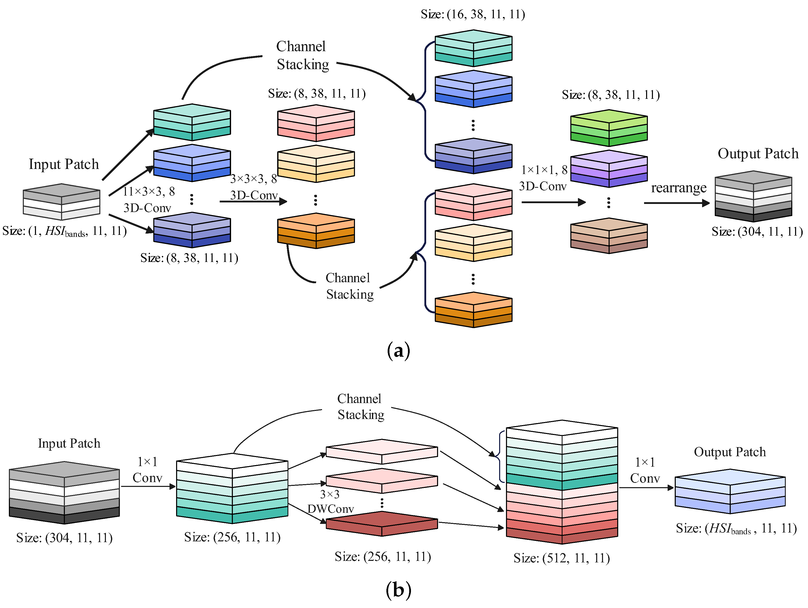
• A spatial-spectral extraction block (SSEB) module for efficient extraction of spatial-spectral features is suggested, to extract deep spatial-spectral features and localized spatial-spectral features using a 3D-convolution module and a 2D-convolution module, respectively.
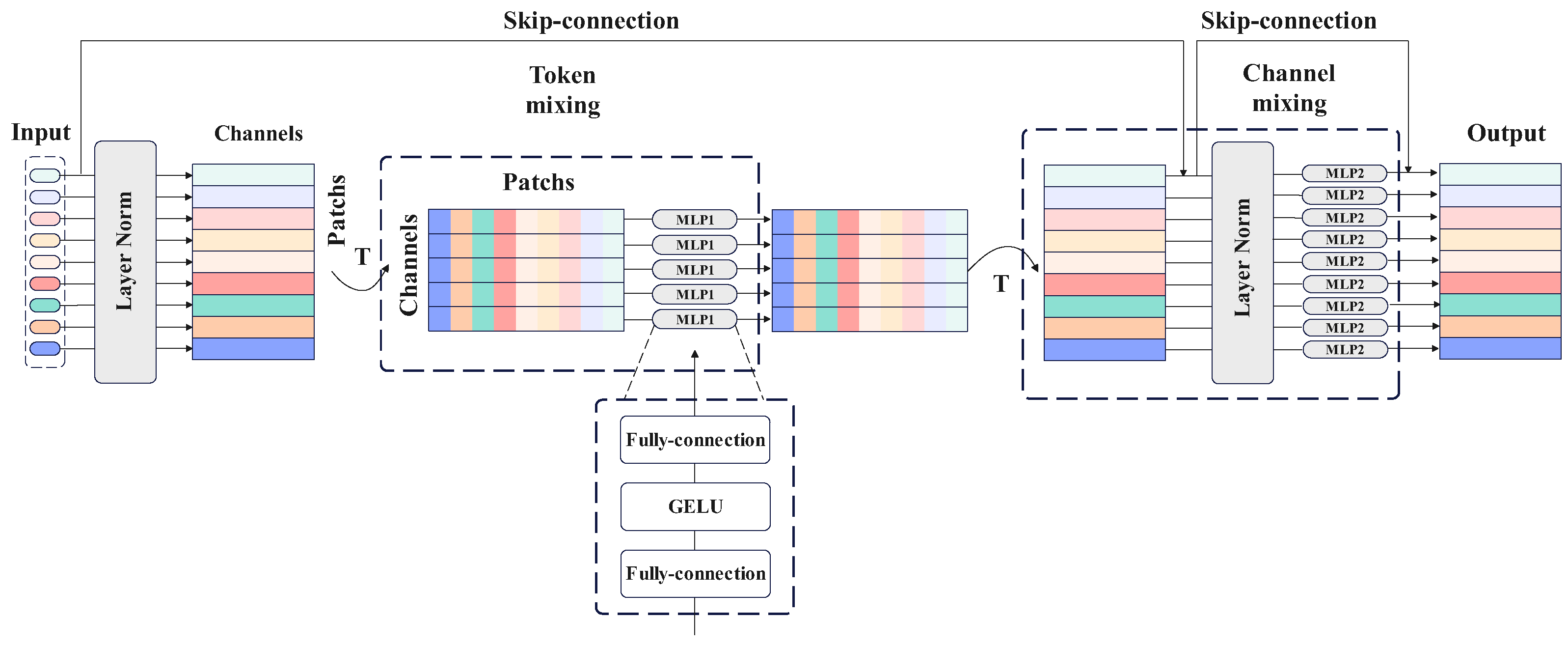
• The spatial spectral features obtained from the SSEB are further mined using the token-mixing MLP module and channel-mixing MLP module of the MLP-mixer, respectively, and feature maps containing more information are obtained under the condition that the output feature maps are guaranteed to be unchanged from the output.
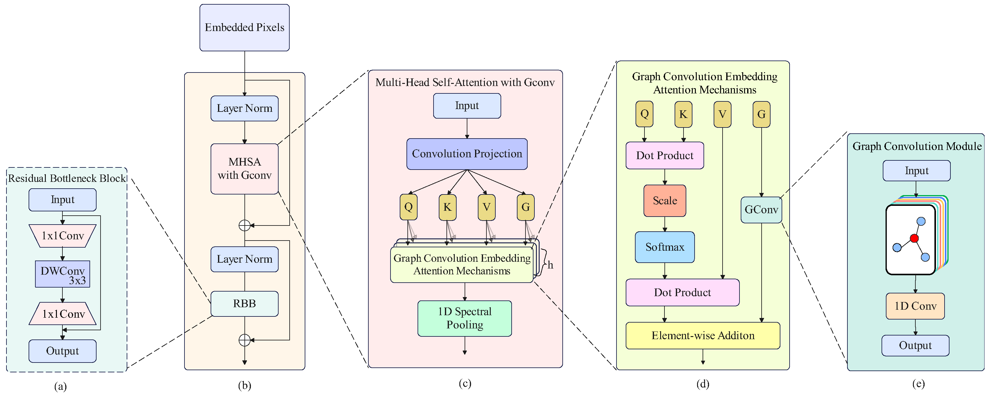
• The graph convolutional enhanced transformer (GCET) introduces graph convolutional into the ViT, which overcomes the shortcomings of MHSA’s overly dispersed attention, while fully exploiting the spatial relationships and similarities between pixels.
• MGCET was subjected to a large number of ablation and comparison experiments on four datasets. The results showed that MGCET had good classification accuracy compared to several state-of-the-art approaches.

2. Methodology

In this section, the MLP-mixer and graph convolutional enhanced transformer for hyperspectral image classification are introduced. Section 2.1 describes the overall network structure. Section 2.2, Section 2.3 and Section 2.4 provide the basic structure and principles of the spatial-spectral extraction block module, MLP-mixer module, and graph convolutional enhanced transformer, respectively. The flowcharts, algorithms, and working steps of the models can be found in Section 2.5.

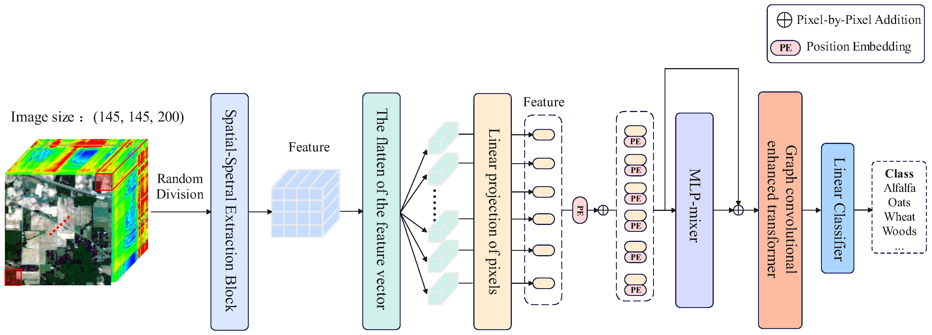
2.1. Overview of MLP-mixer and Graph Convolutional Enhanced Transformer

In this study, a multi-paradigm fusion network (i.e., MGCET) is presented. The MGCET consists of three modules: the SSEB, the MLP-mixer, and the GCET. The SSEB and MLP-mixer are employed to acquire local-global spatial-spectral features, and the GCET improves the modeling of similar relationships between pixels by embedding graph convolution. The specific structure of the MGCET is presented in Figure 1. Taking Indian Pines as an example, first, a certain percentage (e.g., 5%) of pixels from each type of object in the HSI is selected according to a class-randomization-based method, and based on this, the HSI is segmented into 3D-patches with the same size, and then the local spatial-spectral features are extracted by the SSEB. Second, the 3D data are transformed to 2D data by the rearrange and flatten layer, then projected onto the input dimension of the MLP-mixer using a linear layer. The position information of the sequence data is obtained by adding position embedding, and then different types of features are successively extracted by the MLP-mixer and GCET. Finally, a classifier is employed to obtain the final classification results.

2.2. Spatial-Spectral Extraction Block

To extract deep localized spatial-spectral features, we designed a spatial-spectral extraction block (SSEB), as shown in Figure 2. Specifically, the SSEB is divided into a 3D convolution block and a 2D convolution block. The input patch X is first entered into the 3D convolutional layer, where the channel dimension is increased through the use of a 11 × 3 × 3 3D convolutional layer. The spatial-spectral features are then extracted through the use of a 3 × 3 × 3 3D convolutional layer. Finally, the previously obtained features are reused by stacking the previously obtained features. The expression can be written as follows:

$$Z_{out}=3DCon{v}_3\left(Concat\left(3DCon{v}_1\left(X\right),3DCon{v}_2\left(3DCon{v}_1\left(X\right)\right)\right)\right)$$

(1)

where $Z_{out}$ denotes the output of the 3D convolutional model. Concat denotes the stacking of features on the channel dimension. The three 3D convolutional layers $3DCon{v}_1$, $3DCon{v}_2$, and $3DCon{v}_3$ are the three 3D convolutional layers in Figure 2a, in that order.

In the case of the subsequent 2D convolution, the output of the 3D convolution must be rearranged in order to transform its dimensions. Similarly to in the 3D convolution module, the spectral dimensions of the input features are first increased using 1 × 1 convolutional layers. Secondly, local features are extracted using 3 × 3 depth-wise convolution (DWConv), and finally, the local spatial-spectral features are fully extracted by stacking the previously obtained features. The expression is as follows:

$$\begin{array}{cc}\hfill Z_{PW}=& PWCon{v}_1\left(reaarange\left(Z_{out}\right)\right)\hfill \\ \hfill Z_{DW}=& DWCon{v}_1\left(Z_{PW}\right)\hfill \\ \hfill Z_{sseb}=& PWCon{v}_2\left(Concat\left(Z_{PW},Z_{DW}\right)\right)\hfill \end{array}$$

(2)

where $Z_{sseb}$, $Z_{PW}$, and $Z_{DW}$ represent the output of SSEB, PW layer, and DW layer, respectively. $rearrange$ refers to the transform input feature dimension. $PWCon{v}_1$ denotes the point-wise convolution layer with output channel 256. $PWCon{v}_2$ output channel is the same as the spectral dimension of the patch. $Concat$ indicates that the outputs of $PWCon{v}_1$ and $DWConv$ are stacked in the channel dimension.

2.3. MLP-mixer

Deep learning network architectures contain two main types of feature extraction layers: (i) mixing features for a given spatial location, (ii) mixing features between different spatial locations, or both at the same time are functions of different layers in modern deep learning architectures. For instance, CNNs can be implemented with N × N (N > 1) convolution and pooling for (ii), with 1 × 1 convolution for (i), or using larger convolution kernels for (i) and (ii). In ViT or other approaches based on attentional mechanisms, the realization of (i) and (ii) can be achieved through self-attention. The particular structure can be visualized in Figure 3.

The MLP-mixer takes sequence data $X_{N\times D}$ as input data, where N refers to the sequence data length and D denotes the number of sequence data channels. The multilayer perceptron (MLP) component within the MLP-mixer model comprises two fully connected layers and an activation function designated as GELU. Two MLP modules are employed: a token-mixing MLP to act on the columns of X to map ${\mathbb{R}}^N$ to ${\mathbb{R}}^N$, and a channel-mixing MLP to act on the rows of X to map ${\mathbb{R}}^D$ to ${\mathbb{R}}^D$. Additional components include skip-connections, dropout, and layer normalization applied to the module. The MLP-mixer expression is expressed as follows:

$$\begin{array}{cc}\hfill Z_{token}=& X+W_2\sigma \left(W_{1}LayerNorm\left(X\right)\right)\hfill \\ \hfill Z_{mixer}=& Z_{token}+W_4\sigma \left(W_{3}LayerNorm\left(Z_{token}\right)\right)\hfill \end{array}$$

(3)

where $W_1$, $W_2$, $W_3$, and $W_4$ denote the four fully connected layers, and $\sigma$ denotes the activation function GELU. X, $Z_{token}$, and $Z_{mixer}$ denote the input data, the output of the token-mixing MLP, and the output of the MLP-mixer, respectively.

2.4. Graph Convolutional Enhanced Transformer

An undirected graph $\mathcal{G}=〈\mathcal{V},\mathcal{E}〉$ can be used in GCN to describe the relationship between HSI pixels, effectively establishing the spatial relationship between pixels, which is a good complement to the transformer. The graph convolution module we designed mainly consists of the GConv layer and 1-D convolution layer, as depicted in Figure 4e. The spatial similarity between the input sequence data is first mined by the GConv layer, and then the spectral features are extracted using the 1-D convolutional layer. This process can be briefly represented as

$$Z_{gcm}=Con{v}_{1d}\left(GConv\left(Z_{input}\right)\right)$$

(4)

where $Z_{gcm}$ and $Z_{input}$ denote the output results and input data of the graph convolution module, respectively.

The primary structure of the module is presented in Figure 4b, where the input image patches $X=\left[X_1,\dots ,X_d\right]$ are initially transformed into sequence data $P=\left[P_1,\dots ,P_d\right]\in {\mathbb{R}}^{D\times C}$ by executing a flatten and linear projection operation, a process that can be represented by

$$Z_{seq}=Projection\left(Flatten\left(Zsseb\right)\right)$$

(5)

where D refers to the length of the sequence data and C indicates the number of channels of the sequence data. $Z_{seq}$ and $Z_{sseb}$ are the transformed sequence data and the output of the SSEB module, respectively. The location information of the image patch is of paramount importance for ViT, necessitating the addition of location information to the sequence data P, in order to obtain the input data $Z_{mixer}=Mixer\left(Z_{seq}+Z_{pos}\right)$. Here, $Mixer$ denotes the MLP-mixer module. The output of MHSAG can be expressed in the following form:

$$Z_{get}^{\prime }=MHSAG\left(LN\left(Z_{mixer}\right)\right)+Z_{mixer}$$

(6)

where MHSAG represents the multi-head self-attention (MHSA) of the embedded graph convolution, as shown in Figure 4c. Graph convolution embedding attention mechanisms (GCEA) improve the original self-attention (SA) layer of ViT by utilizing a GCN to boost the feature extraction capability of ViT, and the specific structure is illustrated in Figure 4d. Specifically, the input data P are first projected to higher channel dimensions using convolution and then averaged into four feature vectors having the same channel dimensions, Q, K, V, and G. The GCEA layer is expressed as

$$Z_{attn}=GCEA\left(Q,K,V,G\right)=Softmax\left({\displaystyle \frac{Q{K}^T}{\sqrt{d}}}\right)+Z_{gcm}$$

(7)

where $Z_{attn}$ denotes the output of GCEA. Multiple GCEAs can be spliced into a larger attention matrix, e.g., when the heads are equal to 4, this can be denoted as $Z_{attn}^{\left(heads\right)}\left(heads=1,\dots ,4\right)$. To maintain the consistency between the input data and the output data, $Z_{attn}^{\left(heads\right)}$ can be mapped to match the dimensions of input features using a 1-D pooling layer.

Lastly, the RBB (residual bottleneck block) is utilized to replace the original MLP module in ViT. The feature vectors at each position are nonlinearly transformed so that more nonlinear features are introduced, while reducing the parameters of the network to enhance the effect of feature extraction. The specific structure is shown in Figure 4a. The complete feature extraction process of the graph convolutional enhanced transformer encoder can be summarized as follows:

$$Z_{get}=RBB\left(LN\left(Z_{get}^{\prime }\right)\right)+Z_{get}^{\prime }$$

(8)

The output of the entire graph convolutional enhanced transformer encoder is represented by $Z_{get}$. In summary, the module offers the following enhancements compared to pure ViT: (1) graph convolution is introduced in the MHSA layer to enhance the feature extraction capabilities of ViT; (2) convolutional projection, instead of pure linear transformation, is performed for the input sequence data; (3) the use of a residual bottleneck block in place of an MLP decreases the number of network parameters; and (4) the use of a 1-D pooling layer ensures that the dimensions of the inputs and outputs features are consistent.

2.5. System Model

The specific parameter settings and flowchart of MGCET are presented in

Table 1. Configuration details of the graph convolutional enhanced transformer.

Module	Layer	Configuration [Output Size] (Kernel)(Stride) (Padding)
3D Convolution Module	3-D Conv-1	[8, 38, 11, 11]; (11, 3, 3); (5, 1, 1); (0, 1, 1)
	3-D Conv-2	[8, 38, 11, 11]; (3, 3, 3); (1, 1, 1); (1, 1, 1)
	3-D Conv-3	[8, 38, 11, 11]; (1, 1, 1); (1, 1, 1); (0, 0, 0)
	Rearrange	[304, 11, 11](–)(–)(–)
2D Convolution Module	2-D Conv-1	[256, 11, 11]; (1 × 1); (1, 1); (0, 0)
	2-D DWConv-2	[256, 11, 11]; (3 × 3); (1, 1); (0, 0)
	2-D Conv-3	[$HS{I}_{bands}$, 11, 11]; (1 × 1); (1, 1); (0, 0)
Patch Embeddings	nn.Flatten()	[121, $HS{I}_{bands}$](–)(–)(–)
	nn.Linear()	[121, 256](–)(–)(–)
Postional Embeddings	nn.Parameter()	[121, 256](–)(–)(–)
MLP-mixer	nn.LayerNorm()	[121, 256](–)(–)(–)
	token-mixing MLP	[121, 256](–)(–)(–)
	nn.LayerNorm()	[121, 256](–)(–)(–)
	channel-mixing MLP	[121, 256](–)(–)(–)
Graph convolutional Enhanced Transformer Encoder	nn.LayerNorm()	[121, 256](–)(–)(–)
	GConv	[121, 512](–)(–)(–)
	MHSAG	[121, 512](–)(–)(–)
	1-D AdaptiveAvgPool	[121, 256](–)(–)(–)
	nn.LayerNorm()	[121, 256](–)(–)(–)
Residual Bottleneck Block	2-D Conv-5	[11, 11, 64]; (1 × 1); (1 × 1); (0, 0)
	2-D DWConv-6	[11, 11, 64]; (3 × 3); (1 × 1); (1, 1)
	2-D Conv-7	[11, 11, 256]; (1 × 1); (1 × 1); (0, 0)
Classifier	Dropout	Output Size: [121, 256]
	Avg Pooling	[1, 256](–)(–)(–)
	nn.LayerNorm()	[1, 256](–)(–)(–)
	nn.Linear()	[1, Classes](–)(–)(–)

and Figure 5, respectively. The overall workflow of MGCET is summarized into the following eight steps:

1: 

Split HSI dataset $X\in {\mathbb{R}}^{H\times W\times \mathrm{C}}$ into 3D-patches with the same size.

2: 

Spatial-spectral extraction block is utilized to obtain feature $Z_{sseb}$.

3: 

Flattened and projected feature $Z_{sseb}$ to obtain sequence data $Z_{seq}$.

4: 

The spatial and channel features are further extracted using a token-mixer MLP and channel-mixer MLP, respectively, to obtain the feature $Z_{mixer}$.

5: 

The graph convolution module embedded in MHSA is employed to obtain a feature $Z_{gcm}$, which contains the similarity between the sequence data.

6: 

Output features $Z_{attn}$ of MHSAG: $Softmax\left({\displaystyle \frac{Q{K}^T}{\sqrt{d}}}\right)+Z_{gcm}$.

7: 

Feature $Z_{get}$ is the final output of the entire model.

8: 

The final classification result $Z_{out}$ is obtained through AvgPooling and a linear classifier.

3. Experiments

This section is divided into four main parts. Section 3.1 describes several well-known public HSI datasets used in the experiment, as well as the specific division of the training and test sets. Section 3.2 describes the model used to conduct the comparison experiments and the associated experimental setup details. Section 3.3 introduces the metrics used to measure the performance of the model. Section 3.4 details the relevant comparison experiments.

3.1. Dataset Description

In order to validate the effectiveness of the proposed model, correlation experiments were conducted on four common hyperspectral datasets. The four datasets utilized in this study were the Indian Pines (IP), Pavia University (PU), Salinas Valley (SA), and Kennedy Space Center (KSC) datasets.

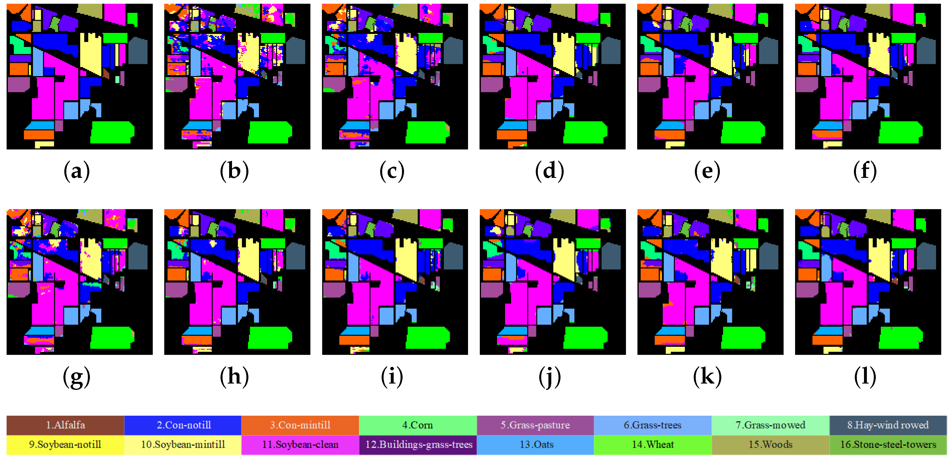
3.1.1. Indian Pines (IP) Dataset

The IP dataset is an HSI image dataset that was collected using an airborne visible infrared imaging spectrometer (AVIRIS) over a site in northwestern Indiana, USA, in June 1992. It covers 145 × 145 (spatial dimensions) for an agricultural area and has 200 spectral bands with a 0.4 to 2.5 $\mathsf{\mu }$m wavelength range and 10,249 labeled pixels. The study area has 16 classes, including corn, oats, wheat, and wood. We randomly selected 5% samples from each category of the IP dataset as the training set, with the remainder as the test set. The number of training and testing samples for each category of the IP dataset can be found in

Table 2. The sample numbers for each class in the experiment stages (training and testing) for the IP dataset with the corresponding color background of each class.

Class No.	Class Name	Training	Testing
1	Alfalfa	2	44
2	Con-notill	71	1357
3	Con-mintill	41	789
4	Corn	12	225
5	Grass-pasture	24	459
6	Grass-trees	37	693
7	Grass-pasture-mowed	1	27
8	Hay-windrowed	24	454
9	Oats	1	19
10	Soybean-notill	49	923
11	Soybean-mintill	123	2332
12	Soybean-clean	30	563
13	Wheat	10	195
14	Woods	63	1203
15	Buildings-grass-trees-drivers	19	367
16	Stone-steel-towers	5	88
Total		512	9737

; the colored background indicates the color of the category in the image.

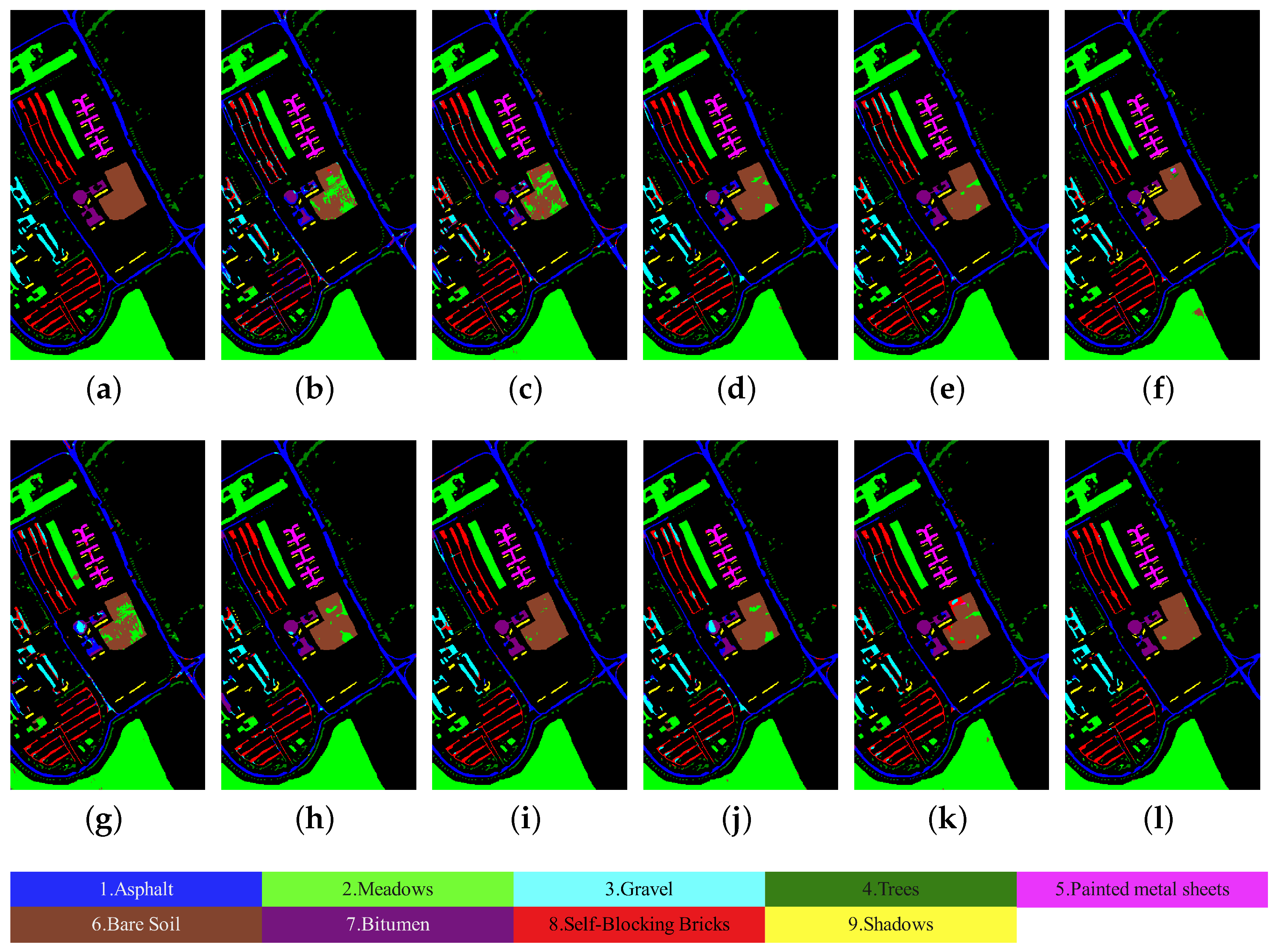
3.1.2. Pavia University (PU) Dataset

The PU dataset covers the city of Pavia and its surrounding areas in Italy. It was captured using a different sensor called the Reflective Optics Spectrographic Imaging System (ROSIS) onboard an airborne sensor platform. The spatial size of the Pavia University dataset is 610 × 340, and its approximate spatial resolution is 1.3 m. Outside of the background pixels (unlabeled pixels), there are 42,776 labeled pixels covering nine classification objects. The dataset has 103 bands (after removing 12 high noise bands).

Table 3. The sample numbers for each class in the experiment stages (training and testing) for the PU dataset, with the corresponding color background of each class.

Class No.	Class Name	Training	Testing
1	Asphalt	66	6565
2	Meadows	186	18,463
3	Gravel	21	2078
4	Trees	31	3033
5	Painted metal sheets	13	1332
6	Bare Soil	50	4979
7	Bitumen	13	1317
8	Self-Blocking Bricks	37	3645
9	Shadows	10	937
Total		427	42,349

gives specific information about the PU dataset.

3.1.3. Salinas Valley (SA)

The Salinas dataset was acquired using the AVIRIS sensor over the Salinas Valley, California. The spatial resolution of the dataset is 3.7 m, its data size is 512 × 217, and it contains 204 continuous bands. There are 16 feature types, including vineyard fields, vegetables, and bare soils.

Table 4. The sample numbers for each class in the experiment stages (training and testing) for each class for SA dataset with the corresponding colored background in the classification map.

Class No.	Class Name	Training	Testing
1	Brocoli-green-weeds-1	20	1989
2	Brocoli-green-weeds-2	37	3689
3	Fallow	20	1956
4	Fallow-rough-plow	14	1380
5	Fallow-smooth	27	2651
6	Stubble	39	3920
7	Celery	36	3543
8	Grapes-untrained	113	11,158
9	Soil-vinyard-develop	62	6141
10	Corn-senesced-green-weeds	33	3245
11	Lettuce-romaine-4wk	11	1057
12	Lettuce-romaine-5wk	19	1908
13	Lettuce-romaine-6wk	9	907
14	Lettuce-romaine-7wk	11	1059
15	Vinyard-untrained	72	7196
16	Vinyard-vertical-trellis	18	1789
Total		541	53,588

details the number of training and testing sets selected, as well as the colors represented by the different categories in the classification map.

3.1.4. Kennedy Space Center (KSC)

AVIRIS acquired the KSC dataset for the Kennedy Space Center in Florida, United States of America, 1996. The spatial dimensions of this image are 512 by 614 (spatial dimensions), and its resolution is 18 m. The precise count of bands is 176 (spectral bands) after eliminating the low signal-to-noise and absorption bands. The studied area comprises thirteen distinct classes, such as slash pine, cabbage palm hammock, willow swamp, and scrub. The category information in the dataset is presented in

Table 5. The sample numbers for each class in the experiment stages (training and testing) for KSC dataset with the corresponding colored background in the classification map.

Class No.	Class Name	Training	Testing
1	Scrub	38	723
2	Willow Swamp	12	231
3	CP Hammock	13	243
4	Slash Pine	13	239
5	0ak/Broadleaf	8	153
6	Hardwood swamp	11	218
7	Swap	5	100
8	Graminoid Marsh	22	409
9	Spartina Marsh	26	494
10	Cattail Marsh	20	384
11	Salt Marsh	21	398
12	Mud Flats	25	478
13	Water	46	881
Total		260	4951

, in which the colored background indicates the color of the category in the classification map.

3.2. Experimental Settings

The settings of the experiments were modified to be 0.001, 200, 100, and 11 × 11 for the learning rate, epoch, batch size, and patch size, respectively. All methods used in the experimental comparison were trained ten times to ensure the fairness of the experiments. In the random division step, for small sample datasets such as IP and KSC, in order to ensure that the number of training samples met the training requirements, we randomly selected 5% samples from each category of the IP and KSC datasets as the training set, with the remaining samples as the test set. Similarly, for large sample datasets such as PU and SA, 1% of the samples were used as training objects, with the remaining 99% as test objects [47,48,49]. Furthermore, the means and standard deviations of overall accuracy (OA), average accuracy (AA), and kappa coefficient (kappa) were obtained for evaluation. The cross-entropy loss function was employed to assess the degree of correspondence between the predicted and actual values throughout the training phase. In order to circumvent overfitting, we opted to uniformly utilize adaptive moment estimation (Adam) as the optimizer. The MGCET algorithm was tested against 10 HSI classification algorithms for the classification performance under four publicly available HSIs. All of the above experiments were implemented on a computer equipped with an i5-13400F, RTX 3090, and 32 GB of RAM. The experiments were conducted 10 times using the PyTorch deep learning framework, and the average was taken as the result of the experiments.

(1) 

SVM-RBF: As a traditional machine learning method, it employs a nonlinear mapping through radial basis function (RBF) for extracting the spectral information of HSI and then selects the optimal penalty coefficients and kernel function parameter through a grid search.

(2) 

3D-CNN: The 3D-CNN model comprises two 3D-CNN with 3 × 3 × 3 convolution kernels, three 3D-CNN with 3 × 1 × 1 convolution kernels, one 3D-CNN with 2 × 3 × 3 convolution kernel, four ReLU activation layers, and a fully connected layer.

(3) 

RSSAN (residual spectral-spatial attention network) is comprised of two primary modules: the spectral-spatial attention learning module, and the spectral-spatial feature module. The former incorporates spatial and spectral attention, while the latter comprises two residual spectral spatial attention modules (containing two convolutional layers and one attention layer).

(4) 

DBDA (double-branch dual-attention mechanism network) mainly consists of spectral and spatial branches. The former comprises a series of three-dimensional convolutional layers and channel attention, while the latter comprises a series of 3D convolutional layers and spatial attention.

(5) 

SSRN (spectral-spatial residual network) is comprised of two blocks for spectral residuals and the same for spatial residuals. The former comprises 3D convolutional layers with a 1 × 1 × 7 kernel size and residuals. Similarly, the latter comprises 3D convolutional layers with a 3 × 3 × 128 kernel size and residuals.

(6) 

ViT (vision transformer) divides an image into patches, subsequently employing the linear embedding sequences of these image blocks as input to the transformer for the purpose of training an image classification model in a supervised manner.

(7) 

SSFTT (spectral-spatial feature tokenization transformer) is comprised of three modules: a spectral-spatial feature extraction, a Gaussian weighted feature tokenizer, and a transformer encoder. The MHSA in the transformer encoder has four heads with an embedding dimension of 256.

(8) 

GAHT: Group-aware hierarchical transformer comprises three grouped pixel embedding and three transformer encoders. The heads of the MHSA in the transformer encoder are 8, 4, 2, with embedding dimensions of 256, 128, 64.

(9) 

SpectralFormer: SpectralFormer primarily comprises two modules: the groupwise spectral embedding and the cross-layer adaptive fusion. The embedding dimensions are 256.

(10) 

IFormer: IFormer primarily consists of a ghost module and inception transformer encoder. The inception transformer encode includes high-frequency feature extraction, low-frequency feature extraction, and feature fusion. The embedding dimensions of the transformer encode are 256.

(11) 

MGECT: MLP-mixer and transformer fusion network is mainly composed of a joint GCN and transformer (JGT) structure, the MLP-mixer module, and a spatial-spectral feature extraction module. The JGT consists of a residual bottleneck block and a transformer encoder with graph convolution embedding. The MHSA in the transformer encoder has four heads, with an embedding dimension of 256.

3.3. Performance Evaluation Indicators

We assessed the performance of the different models by computing OA, AA, and kappa via confusion matrices, and the classification effect was positively correlated with these three indices (OA, AA, kappa ∈ [0, 1]). In the following expressions for OA, AA, and kappa, C denotes the number of species sampled in the HSI dataset, M denotes the number of samples, A denotes the confusion matrix for the prediction results, $A_{ii}$ denotes the value on the diagonal in the confusion matrix (the number of correct classifications), and $A_{ij}$ is the number of samples classifying i as j.

Overall accuracy (OA) indicates the proportion of correctly classified samples out of the total samples, reflecting the algorithm’s overall classification performance. The formula for OA is as follows:

$$OA={\displaystyle \frac{1}{M}}\sum _{i=1}^C{A}_{ii}$$

(9)

Average accuracy (AA) represents the average classification accuracy for each category in the dataset, reflecting the model’s performance on individual categories. The formula for AA is as follows:

$$AA={\displaystyle \frac{1}{C}}\sum _{i=1}^C\left(A_{ij}/\sum _{j=1}^C{A}_{ij}\right)$$

(10)

With an unbalanced number of samples of different classes in the dataset, Kappa is able to comprehensively evaluate the classification effects in terms of both model stability and validity. The expression can be written as follows:

$$Kappa={\displaystyle \frac{\left(\left.M\left({\displaystyle \sum _{i=1}^C}{A}_{ii}-{\displaystyle \sum _{i=1}^C}Aij{\displaystyle \sum _{i=1}^C}{A}_{ji}\right)\right)\right.}{\left(\left.M^2-{\displaystyle \sum _{i=1}^C}\left({\displaystyle \sum _{i=1}^C}{A}_{ij}{\displaystyle \sum _{i=1}^C}{A}_{ji}\right)\right)\right.}}$$

(11)

3.4. Experimental Results and Analysis

3.4.1. Results of Comparative Experiments

The performance of MGCET with traditional machine learning, deep learning methods, and new methods proposed in recent years on HSI datasets such as IP, SA, PU, and KSC is presented in

Table 6. IP dataset classification results.

Class No.	SVM-RBF	3D-CNN	RSSAN	DBDA	RSSN	ViT	SSFTT	GAHT	Spectral Former	iFormer	MGCET
1	71.36 ± 3.65	81.01 ± 3.10	78.29 ± 1.34	76.00 ± 2.01	75.91 ± 2.74	74.52 ± 4.06	77.11 ± 0.70	79.63 ± 0.32	70.52 ± 3.15	76.48 ± 3.35	79.08 ± 1.03
2	68.16 ± 7.99	71.18 ± 6.81	87.69 ± 1.44	83.28 ± 9.17	84.61 ± 7.02	81.89 + 3.72	89.08 ± 1.87	91.30 ± 0.88	86.89 ± 5.53	93.19 ± 4.14	94.70 ± 1.51
3	61.12 ± 5.52	66.92 ± 8.72	89.87 ± 0.45	88.17 ± 6.21	81.39 ± 5.31	79.46 ± 8.19	92.87 ± 3.21	93.59 ± 0.86	91.30 ± 3.83	92.51 ± 0.23	93.30 ± 1.61
4	60.90 ± 11.75	68.89 ± 2.40	90.98 ± 1.99	100.00 ± 0.00	96.42 ± 0.91	85.51 ± 4.89	98.55 ± 0.41	97.71 ± 1.61	95.53 ± 2.34	87.29 ± 3.03	94.48 ± 0.93
5	73.18 ± 0.69	73.36 ± 6.93	93.23 ± 1.29	95.52 ± 5.21	97.05 ± 0.17	85.75 ± 3.16	97.12 ± 1.84	96.19 ± 1.08	87.51 ± 4.01	95.47 ± 3.61	95.25 ± 1.01
6	91.13 ± 1.14	88.29 ± 4.15	96.61 ± 0.37	97.37 ± 1.13	97.42 ± 1.11	81.81 ± 7.71	96.37 ± 0.93	96.71 ± 1.15	99.32 ± 0.13	99.16 ± 0.66	99.36 ± 0.39
7	64.18 ± 10.37	75.00 ± 2.11	76.87 ± 3.62	83.24 ± 1.47	79.30 ± 0.71	75.48 ± 4.01	79.70 ± 0.31	76.87 ± 1.67	84.81 ± 5.01	84.81 ± 11.08	83.69 ± 0.04
8	95.79 ± 1.35	97.02 ± 1.00	97.00 ± 0.00	98.77 ± 0.78	100.00 ± 0.00	73.76 ± 5.72	98.47 ± 0.48	99.05 ± 0.21	83.18 ± 7.78	99.76 ± 0.32	97.90 ± 2.12
9	58.17 ± 1.37	78.00 ± 0.71	75.00 ± 0.33	79.90 ± 0.04	77.29 ± 1.20	83.76 ± 4.72	77.36 ± 4.27	79.78 ± 3.67	73.76 ± 1.94	77.55 ± 2.51	84.27 ± 3.02
10	66.76 ± 2.69	77.93 ± 3.73	88.39 ± 1.13	86.24 ± 4.53	97.63 ± 0.59	89.30 ± 2.19	92.24 ± 2.33	94.04 ± 1.71	93.77 ± 0.13	97.36 ± 1.28	96.68 ± 1.82
11	73.59 ± 3.41	59.64 ± 3.73	85.79 ± 0.76	83.03 ± 3.39	81.21 ± 6.71	77.68 ± 6.24	84.21 ± 4.91	87.18 ± 1.42	93.17 ± 0.42	96.99 ± 2.11	97.97 ± 1.26
12	56.22 ± 5.87	62.94 ± 5.66	89.16 ± 0.88	86.98 ± 7.12	88.30 ± 4.19	86.36 ± 2.91	92.98 ± 3.72	90.70 ± 0.71	82.48 ± 10.72	93.29 ± 6.13	96.61 ± 2.42
13	86.97 ± 0.51	89.05 ± 0.27	97.00 ± 1.10	96.61 ± 1.53	97.37 ± 2.12	94.62 + 2.16	98.61 ± 1.53	99.02 ± 0.34	90.82 ± 4.73	99.94 ± 0.07	99.95 ± 0.03
14	94.43 ± 0.82	83.13 ± 0.60	92.58 ± 0.13	97.78 ± 0.07	96.67 ± 2.64	93.77 ± 1.41	98.18 ± 0.77	99.03 ± 0.39	81.49 ± 7.17	98.10 ± 1.14	97.69 ± 1.77
15	61.70 ± 2.47	80.43 ± 6.91	88.59 ± 0.69	98.17 ± 0.51	96.90 ± 1.13	96.51 ± 2.38	99.17 ± 0.89	98.16 ± 0.71	91.26 ± 3.61	97.91 ± 1.73	95.35 ± 4.46
16	83.17 ± 8.52	100.00 ± 0.00	92.41 ± 2.10	98.77 ± 0.35	100.00 ± 0.00	94.30 ± 3.26	95.47 ± 2.35	97.47 ± 1.25	100.00 ± 0.00	96.78 ± 2.06	97.72 ± 1.09
OA(%)	76.96 ± 2.25	77.83 ± 1.78	91.66 ± 3.63	91.75 ± 3.84	92.47 ± 2.46	81.96 ± 3.21	92.55 ± 2.81	93.87 ± 0.27	87.76 ± 1.81	94.28 ± 0.76	95.45 ± 0.87
AA(%)	72.30 ± 1.66	79.12 ± 1.21	93.13 + 1.08	94.21 ± 2.47	93.17 ± 0.78	81.55 ± 2.07	93.71 + 1.74	95.23 ± 0.48	87.81 ± 2.01	93.22 ± 2.06	95.35 ± 1.96
Kappa(%)	84.81 ± 3.22	74.38 ± 1.99	89.32 ± 0.78	91.03 ± 3.47	80.03 ± 3.83	85.71 ± 3.29	93.33 ± 3.67	94.15 ± 1.23	84.19 ± 4.22	93.47 ± 2.73	95.22 ± 0.91

,

Table 7. SA dataset classification results.

Class No.	SVM-RBF	3D-CNN	RSSAN	DBDA	RSSN	ViT	SSFTT	GAHT	Spectral Former	iFormer	MGCET
1	79.73 ± 6.65	80.47 ± 4.31	97.81 ± 1.36	98.80 ± 0.51	100.00 ± 0.00	85.47 ± 7.16	100.00 ± 0.00	99.84 ± 0.17	93.17 ± 2.05	98.42 ± 0.65	97.14 ± 3.13
2	89.09 ± 4.99	89.59 ± 3.71	97.97 ± 1.07	98.21 ± 0.19	99.91 ± 0.05	92.59 + 1.96	98.66 ± 0.81	96.12 ± 1.03	97.48 ± 0.59	99.08 ± 0.61	100.00 ± 0.00
3	82.50 ± 6.52	88.17 ± 6.02	96.80 ± 1.41	98.07 ± 0.29	96.61 ± 3.11	88.17 ± 4.49	94.79 ± 2.12	97.59 ± 1.01	95.19 ± 0.86	98.31 ± 0.48	99.46 ± 0.36
4	87.20 ± 6.75	88.89 ± 4.41	95.72 ± 3.01	97.63 ± 1.06	95.81 ± 1.41	88.81 ± 3.19	99.22 ± 0.32	97.91 ± 1.06	92.55 ± 3.04	98.48 ± 0.07	98.73 ± 1.08
5	87.59 ± 3.69	90.99 ± 3.51	95.14 ± 4.19	96.21 ± 3.41	96.51 ± 1.97	87.99 ± 5.06	95.59 ± 0.81	98.48 ± 1.03	91.20 ± 2.71	95.47 ± 1.10	98.94 ± 1.13
6	88.69 ± 3.24	93.65 ± 3.19	98.65 ± 1.37	99.07 ± 0.33	97.99 ± 1.61	93.65 ± 2.17	98.69 ± 1.03	100.00 ± 0.00	96.42 ± 1.36	98.15 ± 0.06	99.86 ± 0.15
7	89.95 ± 1.37	93.61 ± 5.22	98.99 ± 0.63	96.89 ± 2.01	98.45 ± 0.79	89.61 ± 2.11	99.10 ± 0.11	98.18 ± 1.77	92.25 ± 2.91	99.19 ± 0.28	99.96 ± 0.03
8	75.58 ± 7.15	86.04 ± 7.01	92.27 ± 4.88	94.77 ± 3.04	93.33 ± 2.70	91.04 ± 1.02	85.59 ± 3.08	92.18 ± 3.01	81.97 ± 3.01	93.14 ± 3.29	94.02 ± 2.52
9	92.73 ± 4.37	96.46 ± 1.02	99.36 ± 0.04	99.95 ± 0.03	98.60 ± 0.28	89.46 ± 2.02	97.91 ± 2.07	98.97 ± 0.16	91.76 ± 3.91	99.15 ± 1.15	99.87 ± 0.12
10	85.95 ± 3.29	91.52 ± 2.35	95.63 ± 1.71	96.01 ± 3.38	98.34 ± 0.99	92.51 ± 2.51	93.51 ± 3.13	97.08 ± 1.74	86.64 ± 6.01	93.47 ± 2.84	97.54 ± 1.68
11	90.58 ± 2.41	93.73 ± 2.03	96.57 ± 1.71	94.23 ± 4.03	97.01 ± 2.79	95.73 ± 0.54	96.70 ± 1.92	99.26 ± 0.49	87.05 ± 1.49	97.62 ± 1.69	99.18 ± 0.36
12	93.24 ± 3.15	96.92 ± 2.36	99.32 ± 0.71	98.98 ± 0.02	98.19 ± 0.29	94.92 ± 1.19	98.88 ± 1.02	99.44 ± 0.61	95.47 ± 0.74	99.06 ± 0.53	99.95 ± 0.06
13	94.37 ± 1.31	97.18 ± 0.81	99.81 ± 0.08	97.79 ± 1.04	97.57 ± 1.08	94.88 + 0.12	96.88 ± 0.58	95.79 ± 1.24	92.61 ± 0.82	95.28 ± 1.37	100.00 ± 0.00
14	95.35 ± 1.02	90.82 ± 2.11	95.97 ± 2.03	96.08 ± 1.02	98.57 ± 0.66	90.82 ± 3.10	91.80 ± 1.07	97.57 ± 1.59	97.97 ± 1.16	96.51 ± 1.48	99.20 ± 0.51
15	73.66 ± 8.07	68.08 ± 4.99	85.05 ± 3.03	87.17 ± 3.59	85.68 ± 6.23	75.08 ± 9.08	84.42 ± 6.09	91.28 ± 3.72	79.07 ± 8.31	90.65 ± 2.37	92.76 ± 2.75
16	96.08 ± 3.22	96.86 ± 0.11	99.91 ± 0.10	92.72 ± 0.41	98.46 ± 0.44	94.76 ± 0.26	96.09 ± 1.55	96.87 ± 1.65	87.12 ± 3.05	94.13 ± 2.71	99.37 ± 0.61
OA(%)	86.64 ± 4.05	89.20 ± 3.17	94.74 ± 2.93	95.25 ± 1.89	95.73 ± 1.06	90.20 ± 1.28	93.53 ± 1.13	96.48 ± 1.22	91.32 ± 1.81	95.28 ± 0.37	97.52 ± 0.37
AA(%)	84.46 ± 4.61	90.91 ± 2.75	95.77 + 2.12	96.01 ± 1.38	96.17 ± 0.78	92.19 ± 3.01	95.08 + 0.74	96.89 ± 1.08	93.48 ± 2.01	95.74 ± 1.20	98.52 ± 0.34
Kappa(%)	85.24 ± 1.52	90.19 ± 4.09	95.76 ± 2.18	95.26 ± 0.78	91.11 ± 2.38	94.01 ± 1.92	96.44 ± 0.69	95.34 ± 1.23	90.34 ± 3.89	94.68 ± 0.71	97.04 ± 0.41

,

Table 8. PU dataset classification results.

Class No.	SVM-RBF	3D-CNN	RSSAN	DBDA	RSSN	ViT	SSFTT	GAHT	Spectral Former	iFormer	MGCET
1	82.40 ± 1.81	83.02 ± 2.77	91.93 ± 0.98	93.54 ± 1.05	94.24 ± 1.08	89.45 ± 2.81	95.61 ± 1.49	95.54 ± 0.23	88.73 ± 0.61	96.01 ± 0.46	97.37 ± 1.64
2	83.34 ± 3.05	88.12 ± 4.17	94.63 ± 0.27	96.43 ± 0.62	98.03 ± 0.89	90.54 ± 4.35	96.36 ± 0.63	97.43 ± 0.71	95.88 ± 0.72	97.75 ± 0.82	99.55 ± 0.53
3	86.37 ± 3.01	84.61 ± 3.82	88.68 ± 2.49	89.44 ± 1.51	90.44 ± 1.12	85.05 ± 6.95	90.38 ± 2.12	92.44 ± 1.37	89.40 ± 2.01	84.11 ± 7.12	93.65 ± 3.77
4	82.92 ± 1.91	90.11 ± 1.44	96.91 ± 1.05	94.93 ± 1.12	94.52 ± 0.51	94.77 ± 0.71	96.36 ± 0.82	96.93 ± 1.30	95.97 ± 1.24	97.92 ± 0.27	97.36 ± 1.14
5	92.03 ± 1.25	93.48 ± 0.92	97.69 ± 0.69	98.07 ± 0.35	98.57 ± 0.61	94.12 ± 0.53	97.68 ± 1.21	98.07 ± 0.71	94.88 ± 1.79	98.39 ± 0.77	99.12 ± 1.10
6	94.21 ± 0.32	81.94 ± 9.12	96.32 ± 2.12	97.72 ± 1.28	96.62 ± 1.47	89.91 ± 1.67	92.37 ± 2.47	97.12 ± 0.44	85.29 ± 3.06	87.26 ± 8.13	97.96 ± 0.42
7	93.81 ± 1.64	86.38 ± 4.02	97.40 ± 1.33	98.71 ± 0.23	97.04 ± 0.96	94.29 ± 2.72	94.49 ± 1.61	98.51 ± 0.35	87.45 ± 3.14	97.12 ± 1.08	98.10 ± 3.51
8	90.46 ± 1.72	95.97 ± 1.59	96.39 ± 1.08	97.37 ± 0.19	97.17 ± 0.62	97.01 ± 1.06	95.94 ± 0.31	98.17 ± 0.17	94.38 ± 1.01	94.96 ± 0.12	96.44 ± 2.49
9	89.82 ± 0.98	93.62 ± 0.92	97.65 ± 0.08	97.97 ± 0.43	98.27 ± 0.59	94.84 ± 1.82	97.31 ± 0.76	98.27 ± 0.11	95.25 ± 1.12	96.95 ± 0.48	97.88 ± 1.70
OA(%)	85.15 ± 1.08	87.74 ± 1.73	95.47 ± 0.72	96.07 ± 0.33	96.57 ± 0.23	91.37 ± 3.17	95.32 ± 0.91	96.47 ± 0.31	92.00 ± 1.42	94.56 ± 0.97	98.05 ± 0.41
AA(%)	89.89 ± 1.11	86.70 ± 3.12	95.91 + 0.95	95.98 ± 0.47	96.38 ± 1.01	92.12 ± 1.99	94.39 ± 1.35	96.28 ± 0.26	91.37 ± 1.92	93.41 ± 1.03	96.99 ± 1.19
Kappa(%)	83.04 ± 1.78	83.69 ± 3.41	93.71 ± 0.58	95.24 ± 0.92	95.64 ± 1.02	90.80 ± 3.08	93.94 ± 3.23	95.74 ± 0.40	92.96 ± 1.91	91.23 ± 0.71	97.56 ± 0.81

and

Table 9. KSC dataset classification results.

Class No.	SVM-RBF	3D-CNN	RSSAN	DBDA	RSSN	ViT	SSFTT	GAHT	Spectral Former	iFormer	MGCET
1	88.40 ± 4.00	93.40 ± 1.30	98.20 ± 0.36	100.00 ± 0.00	99.86 ± 0.12	92.08 ± 0.50	100.00 ± 0.00	99.82 ± 0.21	94.31 ± 0.51	100.00 ± 0.00	100.00 ± 0.00
2	82.28 ± 7.69	86.28 ± 4.69	96.46 ± 1.08	97.42 ± 2.98	97.02 ± 1.82	87.21 ± 3.68	98.66 ± 0.81	99.05 ± 0.72	87.63 ± 2.02	99.24 ± 0.71	96.10 ± 2.72
3	85.80 ± 6.52	85.80 ± 3.71	97.60 ± 2.12	92.61 ± 3.05	97.33 ± 1.51	90.08 ± 7.00	94.79 ± 2.12	98.16 ± 0.71	86.59 ± 1.72	97.97 ± 2.17	98.68 ± 1.21
4	70.71 ± 2.64	75.71 ± 4.77	91.32 ± 3.62	87.32 ± 8.27	92.67 ± 2.62	77.02 ± 9.14	94.22 ± 0.32	88.04 ± 10.09	92.10 ± 3.22	91.32 ± 6.90	92.55 ± 3.46
5	76.22 ± 6.85	69.22 ± 4.64	84.41 ± 6.02	94.41 ± 4.77	86.86 ± 7.05	84.96 ± 8.33	95.59 ± 0.81	90.72 ± 2.21	72.52 ± 8.26	90.55 ± 4.18	88.72 ± 3.21
6	93.34 ± 2.20	87.34 ± 3.85	93.45 ± 4.01	95.01 ± 4.08	93.74 ± 5.59	91.69 ± 3.60	98.69 ± 1.03	92.41 ± 4.12	94.54 ± 2.83	98.54 ± 2.32	97.43 ± 0.81
7	89.34 ± 6.40	94.34 ± 4.20	92.37 ± 5.06	87.37 ± 2.46	97.92 ± 0.52	93.75 ± 0.93	99.10 ± 0.11	94.00 ± 1.24	93.12 ± 3.24	88.62 ± 0.17	99.41 ± 0.39
8	87.75 ± 1.48	89.75 ± 2.09	95.90 ± 0.82	96.90 ± 1.19	98.21 ± 1.62	86.88 ± 4.66	90.59 ± 3.08	99.95 ± 0.19	96.90 ± 0.97	97.33 ± 0.93	99.80 ± 0.08
9	91.01 ± 2.09	95.01 ± 3.40	96.51 ± 1.10	97.01 ± 0.62	99.72 ± 0.26	91.99 ± 3.48	97.91 ± 2.07	100.00 ± 0.00	100.00 ± 0.00	99.19 ± 0.67	99.95 ± 0.07
10	91.63 ± 4.38	93.03 ± 1.08	100.00 ± 0.00	99.76 ± 0.38	99.53 ± 0.50	91.48 ± 0.69	93.51 ± 3.13	99.91 ± 0.29	100.00 ± 0.00	100.00 ± 0.00	100.00 ± 0.00
11	93.93 ± 2.41	95.33 ± 2.19	98.14 ± 0.52	99.61 ± 0.46	98.84 ± 0.70	92.78 ± 4.23	96.70 ± 1.92	98.28 ± 0.02	95.49 ± 0.17	99.29 ± 0.15	99.94 ± 0.10
12	95.56 ± 3.15	92.02 ± 4.38	96.87 ± 1.38	98.87 ± 1.02	97.15 ± 3.02	92.24 ± 2.98	98.88 ± 1.02	100.00 ± 0.00	94.23 ± 2.85	99.56 ± 0.33	99.03 ± 1.04
13	96.32 ± 2.13	98.23 ± 0.81	99.20 ± 0.81	99.82 ± 0.12	100.00 ± 0.00	97.35 ± 3.12	96.88 ± 0.58	100.00 ± 0.00	100.00 ± 0.00	100.00 ± 0.00	100.00 ± 0.00
OA(%)	88.96 ± 1.23	90.97 ± 1.07	96.02 ± 0.41	96.59 ± 0.53	97.03 ± 0.65	90.71 ± 0.83	97.52 ± 0.48	97.77 ± 0.60	93.64 ± 0.82	97.59 ± 0.58	98.52 ± 0.78
AA(%)	86.61 ± 1.88	88.01 ± 2.75	94.56 + 1.12	94.06 ± 1.24	95.26 ± 1.40	88.94 ± 1.17	95.62 + 1.09	96.45 ± 1.18	92.58 ± 1.91	96.88 ± 1.47	97.38 ± 1.60
Kappa(%)	89.94 ± 1.37	91.21 ± 0.29	96.04 ± 1.04	96.21 ± 0.59	96.82 ± 0.73	89.66 ± 0.92	96.95 ± 0.53	97.30 ± 1.23	92.59 ± 0.68	96.02 ± 0.93	98.47 ± 0.86

. Figure 6, Figure 7, Figure 8 and Figure 9 illustrate the classification maps of different models on the same data. As an illustration, Figure 6a depicts the ground truth map for the IP dataset, while Figure 6b–l show the classification maps obtained by different models.

For instance, using the IP dataset, we proportionally selected 5% (512 samples) as the training object and used the remaining 9737 samples as the test set. As illustrated in Table 6, MGCET exhibited a classification accuracy of 97.97% for the 11th category (Soybean-mintill) with the largest number of samples, which was approximately 12% higher than that of RSSAN and GAHT and approximately 5% higher than that of spectral former. Similarly, it was approximately 10% higher than RSSAN and spectral former and approximately 4% higher than GAHT and DBDA in the ninth category (Oats) with the lowest number of samples. The reason why MGCET’s accuracy was better than that of the comparative objects for most of the classified objects was that it was able to fully exploit global and local features by effectively combining multiple network structures, thus improving the recognition ability for difficult-to-classify objects.

Overall, our proposed MGCET outperformed the other methods for OA, AA, and Kappa. Firstly, the SVM and 3D-CNN achieved 76.96% and 77.83%, respectively, which were lower than the other models, indicating the lack of competitiveness of these classical models compared to the other new models. The classification accuracies of ViT and spectral former were 81.96% and 87.76%, respectively, which were approximately 11% and 5% lower than those of hybrid models such as DBDA and SSFTT. This discrepancy was due to the fact that, while ViT has a stronger global feature extraction capability than traditional methods, it lacks the ability to acquire some localized features, which is the reason for the bottleneck in the performance of ViT. The residual CNN models, including RSSAN, DBDA, and SSRN, achieved classification accuracies of 91.66%, 91.75%, and 92.47%, respectively. In comparison, MGCET demonstrated superior classification results. Furthermore, for the other ViT hybrid models (e.g., iFormer, GAHT), MGCET employed the MLP-mixer module to extract the spatial and channel relationship between input pixels, thereby achieving a higher Kappa, OA, and AA.

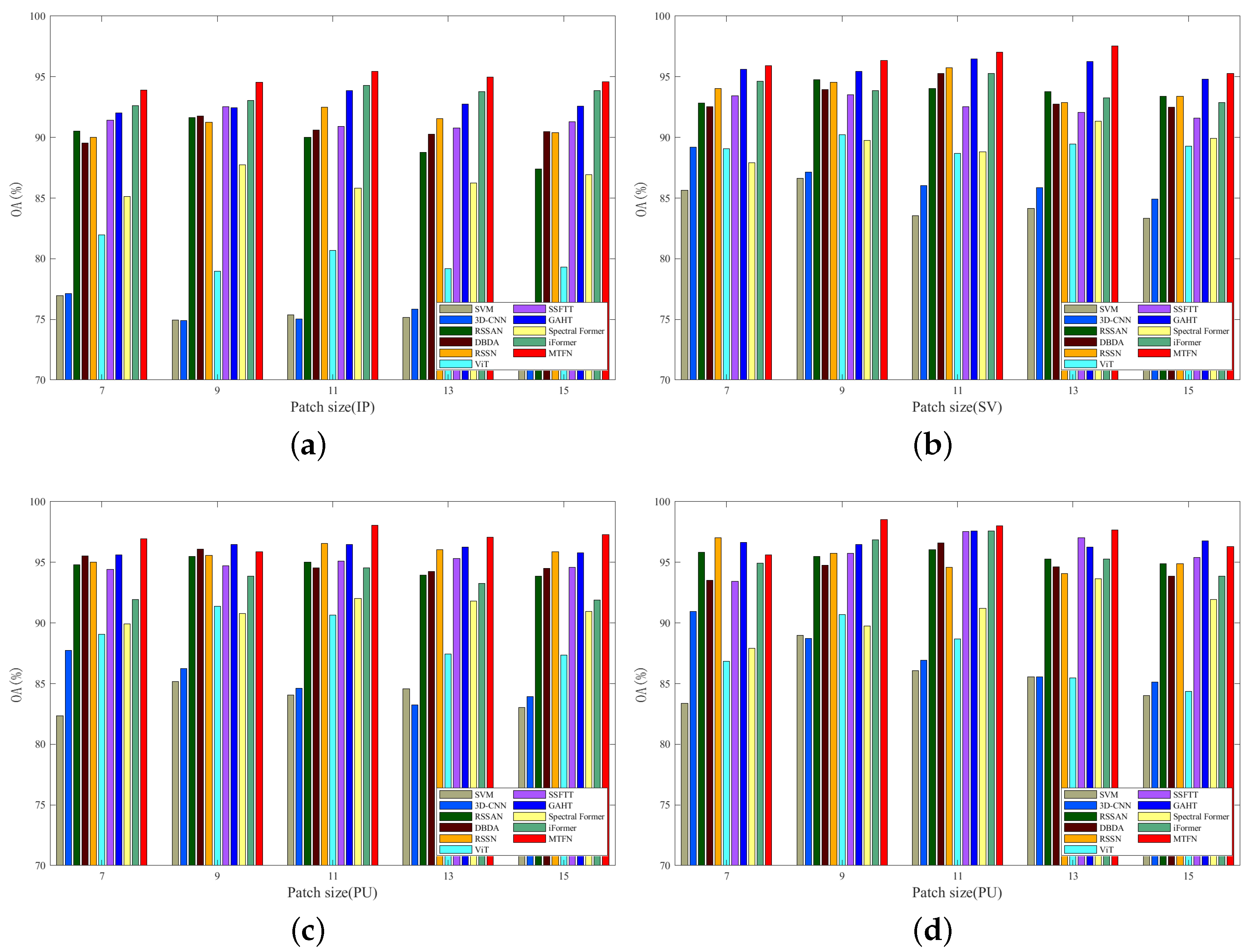
3.4.2. Image Patch Size Analysis

Figure 10a–d illustrates the classification accuracy of the MGCET in comparison to the benchmark model across a range of patch sizes on the IP, SA, PU, and KSC datasets. As shown, the MGCET had a higher OA than the other models in most cases. On most datasets, the OA of most methods did not show a positive correlation with patch size; instead showing a certain degree of decrease. This discrepancy can be attributed to the fact that, while a larger patch size facilitates the acquisition of spatial information, thereby enhancing classification, the same patch may also contain pixels that are elevated in a multiplicative manner, rendering the identification of the target pixel more challenging. It is noteworthy that the MGCET exhibited the highest OA on the IP and PU datasets when the patch size was 11 × 11 and performed well on the remaining datasets.

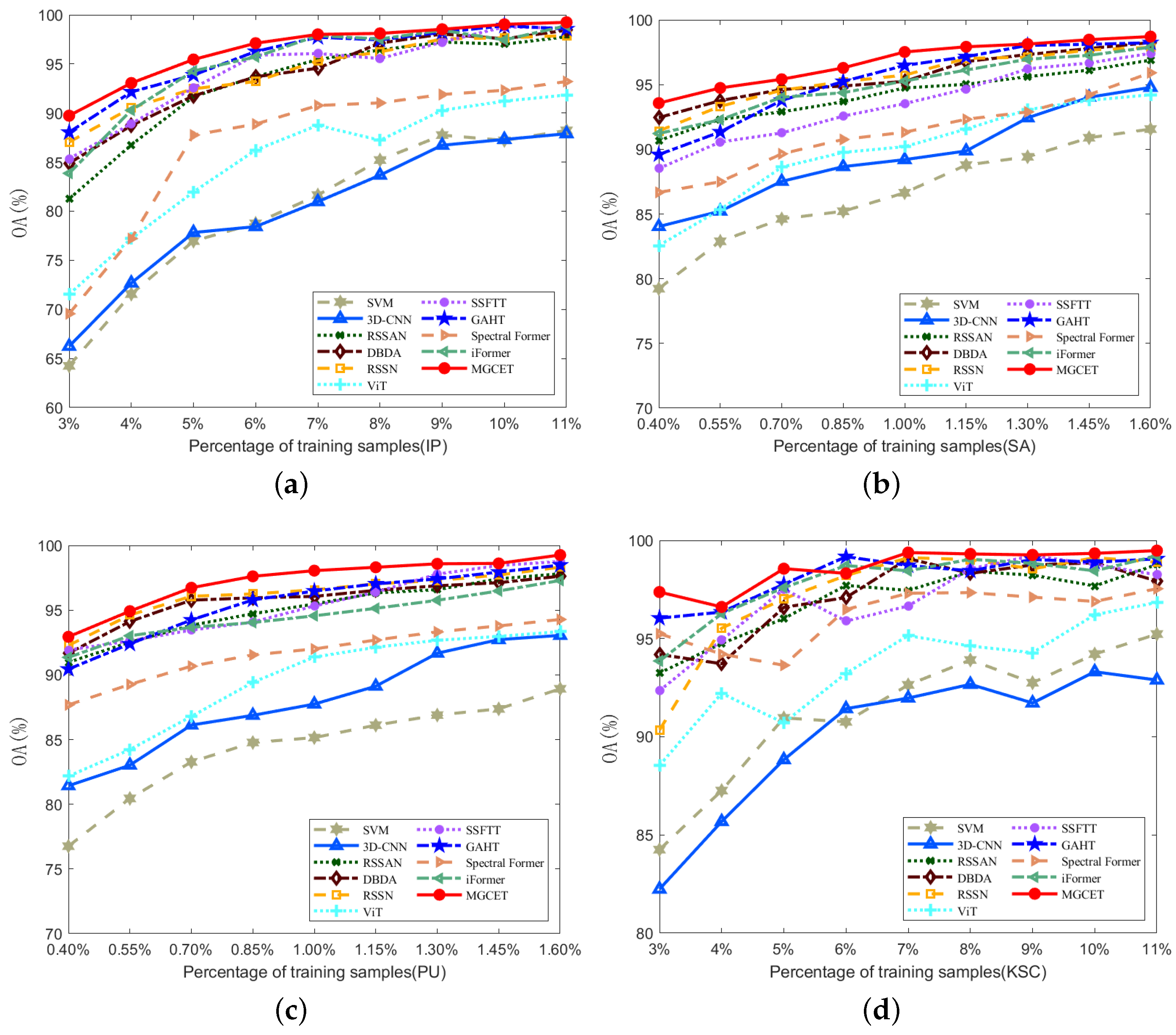
3.4.3. Analysis of Training Samples

As a further analysis, we compared the performance of the MGCET with the other models with a different percentage of training samples. The training samples for the IP dataset and the KSC dataset ranged from 3% to 11% of the dataset, respectively, with an interval of 1%. Similarly, the training samples for the PU and SA datasets ranged from 0.4% to 1.6% of the dataset, respectively, with an interval of 0.15%. Figure 11 shows the OA curves of all models on the IP, PU, SA, and KSC datasets.

As illustrated in Figure 11, an increase in the number of training samples for the four datasets was accompanied by an enhancement in the OA for all models. Upon reaching a specific threshold of training samples, the OA of the majority of models began to fluctuate and exhibit a decline or, in some cases, a complete absence of growth. In general, when the number of training samples was held constant, the OA of MGCET (red dot) was consistently higher than that of the other models, particularly for single CNN models (e.g., RSSAN, 3D-CNN) and pure ViT (e.g., ViT, spectral former). This is primarily attributable to the capacity of MGCET to fully extract both local and global spatial-spectral features through the integration of multiple network modules, which compensated for the inherent limitations of a single network structure in terms of feature extraction capabilities. Furthermore, it is worth mentioning that the MGCET possesses certain advantages over other hybrid models, which can be attributed to the integration of the MLP-mixer.

Figure 12 illustrates the accuracy trends for the four datasets during the training phase of the compared models. Unlike the other models, the proposed model demonstrated remarkable stability and maintained a high accuracy throughout the entire training process. This was particularly evident with the more complex IP and PU datasets, where its performance consistently outpaced that of the other models. The sustained high accuracy and stability suggest that the proposed model did not experience overfitting.

4. Discussion

In this section, we designed and conducted various experiments to analyze the rationality of the proposed MGCET from different perspectives.

4.1. Analysis of Different Modules

The Mlp-mixer and graph convolutional enhanced transformer (GCET) are the key modules of the MGCET. In order to demonstrate that the Mlp-mixer and GCET could effectively improve the results of the model, we performed sufficient ablation experiments on the four datasets introduced above and then evaluated the effectiveness of the added modules using the evaluation indicators. Different modules made up these networks. (1)Net-1: ViT; (2) Net-2: ViT + Mlp-mixer; (3) Net-3: GCET; (4) Net-4: GCET + Mlp-mixer.

The evaluation results of the above model are presented in

Table 10. The ablation results of GCET and Mlp-mixer.

Network	GCET	MLP-mixer	Metric	IP	SA	PU	KSC
Net-1	✕	✕	OA$\left(\%\right)$	83.82 ± 4.76	88.80 ± 1.13	82.22 ± 6.71	90.26 ± 0.71
			AA$\left(\%\right)$	78.18 ± 5.16	89.24 ± 1.58	84.55 ± 4.57	89.76 ± 2.32
			Kappa$\left(\%\right)$	82.20 ± 5.32	88.69 ± 1.32	82.59 ± 4.79	91.25 ± 1.66
Net-2	✕	✓	OA$\left(\%\right)$	93.36 ± 2.08	95.23 ± 0.50	95.52 ± 2.11	96.91 ± 0.42
			AA$\left(\%\right)$	92.05 ± 2.29	96.17 ± 1.51	96.33 ± 0.93	94.78 ± 0.11
			Kappa$\left(\%\right)$	91.57 ± 2.15	95.98 ± 0.68	97.34 ± 1.26	97.12 ± 0.30
Net-3	✓	✕	OA$\left(\%\right)$	94.41 ± 1.18	96.35 ± 0.71	97.21 ± 1.17	97.72 ± 0.18
			AA$\left(\%\right)$	92.45 ± 1.88	96.45 ± 0.31	95.75 ± 0.83	96.30 ± 0.70
			Kappa$\left(\%\right)$	92.49 ± 1.84	95.77 ± 0.86	96.02 ± 1.02	96.91 ± 0.12
Net-4	✓	✓	OA$\left(\%\right)$	95.45 ± 0.91	97.57 ± 0.42	98.05 ± 0.41	98.52 ± 0.07
			AA$\left(\%\right)$	93.99 ± 1.28	97.22 ± 0.60	97.78 ± 0.20	97.74 ± 0.34
			Kappa$\left(\%\right)$	94.73 ± 1.06	97.49 ± 0.68	97.49 ± 0.68	98.04 ± 0.55

, where the various added modules had different degrees of gain for MGCET. First, Net-1 obtained the lowest OA, AA, and Kappa on all datasets. Second, Net-2 performed significantly better than Net-1 on the four datasets, and the classification accuracy of the pure ViT was significantly improved after the introduction of the MLP-mixer, which, side by side, illustrates the contribution of the MLP-mixer to the improvement in classification accuracy. This was due to the fact that the MLP-mixer contains both a token-mixing MLP and channel-mixing MLP, which enables the fusion and interaction of spatial and channel features. Net-3 enhances the feature information acquisition ability of the ViT by replacing the encoder of the ViT with a graph-convolution embedded encoder and adding residual bottleneck blocks, thus achieving an excellent classification accuracy. Finally, Net-4 further improves the classification effect based on Net-2 and Net-3. This is primarily due to the fact that the MGCET is capable of extracting both rich spatial-spectral features and local-global features in HSIs with the assistance of multiple paradigms, such as CNN, Transformer, MLP, and GCN, and it organically fuses them to boost the classification accuracy even further.

To ascertain the contribution of graph convolution to the classification accuracy of the MGCET algorithm, this paper conducted relevant comparison experiments between MHSA and MHSAG on four HSI datasets. As illustrated in

Table 11. Ablation analysis of MHSAG and MHSA.

Network	Metric	IP	SA	PU	KSC
MHSA	OA$\left(\%\right)$	94.92 ± 0.76	96.88 ± 0.83	97.82 ± 0.71	98.36 ± 0.41
	AA$\left(\%\right)$	93.58 ± 0.52	97.04 ± 0.08	96.55 ± 1.07	96.76 ± 0.52
	Kappa$\left(\%\right)$	93.32 ± 1.12	96.69 ± 0.41	96.29 ± 0.72	97.75 ± 0.16
MHSAG	OA$\left(\%\right)$	95.45 ± 0.91	97.57 ± 0.42	98.05 ± 0.41	98.52 ± 0.07
	AA$\left(\%\right)$	93.99 ± 1.28	97.22 ± 0.60	97.78 ± 0.20	97.74 ± 0.34
	Kappa$\left(\%\right)$	94.73 ± 1.06	97.49 ± 0.68	97.49 ± 0.68	98.04 ± 0.55

, the incorporation of graph convolution into MHSA led to a notable enhancement in the OA, AA, and kappa values for all datasets. For instance, the OA was elevated by approximately 0.5% by MHSAG on the IP dataset. This evidence suggests that MGCET is capable of capturing the inherent similarities between sequence data through the embedding of graph convolution, thereby enhancing the model’s capacity to represent features effectively.

4.2. Analysis of Attention Mechanism

Figure 13 demonstrates the classification accuracy of MGCET under different numbers of encoder layers and multiple self-attention layers. On most of the datasets, the OA did not show a corresponding increase with the increase in the number of encoder layers but instead showed a certain degree of decrease. This suggests that model depth does not contribute to the classification accuracy of the MGCET but rather inhibits it to some extent. The number of heads in MHSA did not significantly impact the classification accuracy of the MGCET. In the majority of cases, the classification accuracy of MGCET initially improved and subsequently declined as the number of heads was increased. Overall, the OA exhibited fluctuations as a function of the number of encoder layers and MHSA, yet all stabilized within a stable range. This was observed for the IP dataset (94.83% to 95.45%), the SA dataset (96.67% to 97.57%), the PU dataset (97.36% to 98.05%), and the KSC dataset (98.11% to 98.52%). As illustrated in Figure 13, the MGCET achieved the most optimal classification outcomes on the IP, PU, and KSC datasets when one layer and four heads were selected and on the SA dataset when one layer and five heads were selected. In order to ensure the consistency of training results, the MGCET selected a single layer and four heads in a uniform manner.

4.3. Analysis of Model Architecture

The MLP-mixer and GCET are the key modules of the network architecture, and the way they are connected to each other, as well as the feature fusion method, have an important impact on the model classification effect. In order to prove the rationality of the network architecture proposed in this paper, we proposed four different network architectures based on MLP-mixer and GCET:

• Structure-1: parallel and additive fusion;
• Structure-2: parallel and multiplicative fusion;
• Structure-3: series and MLP-mixer preceded GCET;
• Structure-4: Series and GCET preceded MLP-mixer.

Where Structure-3 is the network architecture used in this paper.

As can be seen in

Table 12. Analysis of Different network architectures.

Structure	Metric	IP	SA	PU	KSC
Structure-1	OA$\left(\%\right)$	94.57 ± 0.76	96.97 ± 0.47	97.59 ± 0.21	97.79 ± 0.65
	AA$\left(\%\right)$	93.51 ± 0.82	97.11 ± 0.24	95.97 ± 0.51	95.97 ± 1.38
	Kappa$\left(\%\right)$	94.13 ± 0.89	96.52 ± 0.52	96.81 ± 0.28	97.53 ± 0.72
Structure-2	OA$\left(\%\right)$	94.29 ± 0.60	96.68 ± 0.83	97.25 ± 0.60	98.01 ± 0.27
	AA$\left(\%\right)$	92.74 ± 1.17	97.31 ± 0.25	95.52 ± 1.02	96.50 ± 1.83
	Kappa$\left(\%\right)$	92.89 ± 0.69	96.31 ± 0.93	96.36 ± 0.80	97.79 ± 1.09
Structure-3	OA$\left(\%\right)$	95.45 ± 0.91	97.57 ± 0.42	98.05 ± 0.41	98.52 ± 0.07
	AA$\left(\%\right)$	93.99 ± 1.28	97.22 ± 0.60	97.78 ± 0.20	97.74 ± 0.34
	Kappa$\left(\%\right)$	94.73 ± 1.06	97.49 ± 0.68	97.49 ± 0.68	98.04 ± 0.55
Structure-4	OA$\left(\%\right)$	95.14 ± 0.31	97.18 ± 0.26	97.78 ± 0.26	98.11 ± 0.41
	AA$\left(\%\right)$	93.66 ± 2.21	97.59 ± 0.16	96.51 ± 0.42	97.35 ± 0.95
	Kappa$\left(\%\right)$	94.80 ± 0.35	96.86 ± 0.28	96.66 ± 0.18	97.78 ± 0.18

, the four network architectures achieved very good classification results on all four publicly available datasets, demonstrating that the combination of GCET and MLP-mixer possesses strong feature extraction capabilities regardless of whether a parallel or serial network architecture is used. In general, the serial network architecture demonstrated superior performance compared to the parallel network architecture. For example, on the IP dataset, Structure-3 and Structure-4 achieved 95.45% and 95.14%, respectively, while Structure-1 and Structure-2 achieved 94.57% and 94.29%. This phenomenon may be attributed to the fact that the multi-branch architectural design diverts the model’s attention from the crucial information that influences the accuracy of the classification, thereby impairing the model’s classification efficacy. The main role of the MLP-mixer is to mine the key spatial-spectral information that affects the classification effect, while GCET is able to continue to acquire the local-global combination of features on the basis of the information acquired by the MLP-mixer, as well as to capture the similarity between the sequence information with the help of graph convolution. In comparison to Structure-3, Structure-4 differs in the sequence of the MLP-mixer and GCET, which has an impact on the model’s classification accuracy. The Structure-3 used in this paper achieved the best performance on all four public datasets, justifying the network architecture proposed in this paper in terms of classification accuracy. In comparison to Structure-1, Structure-2, and Structure-4, Structure-3, as utilized in this paper, exhibited the optimal performance on all four public datasets, thereby substantiating the proposed network architecture from the standpoint of classification accuracy.

5. Conclusions

In order to compensate for the lack of feature extraction capabilities of any single network paradigm, this paper proposed a hybrid network MLP-mixer and graph convolutional enhanced transformer (MGCET) for HSI classification. The network combines four currently dominant network models, including MLP, GCN, CNN, and ViT. Specifically, the CNN and MLP modules are first utilized for spatial-spectral feature extraction. Then, the feature modeling capability of ViT is improved by embedding graph convolution into MHSA to further enhance the classification accuracy of the model. Experimental evaluation on several HSI datasets showed that the combination of multiple network architectures could indeed boost the accuracy of the method, while having a higher classification accuracy compared to the other methods.

A frequent challenge in multi-network architecture models is the competition between different paradigms, which can negatively impact classification accuracy. To address this issue, future research could investigate enhanced network fusion methods and explore incorporating innovative network architectures such as generative adversarial networks (GAN) and the stacked autoencoder (SAE). Alternatively, replacing the original network architectures may offer a potential solution to mitigate this problem. How to reduce the computational complexity of the model through lightweighting techniques is also an important research direction for us.

References

1. Feng, X.; He, L.; Cheng, Q.; Long, X.; Yuan, Y. Hyperspectral and multispectral remote sensing image fusion based on endmember spatial information. Remote Sens. 2020, 12, 1009. [Google Scholar] [CrossRef]
2. Gao, A.F.; Rasmussen, B.; Kulits, P.; Scheller, E.L.; Greenberger, R.; Ehlmann, B.L. Generalized unsupervised clustering of hyperspectral images of geological targets in the near infrared. In Proceedings of the IEEE/CVF Conference on Computer Vision and Pattern Recognition, Nashville, TN, USA, 20–25 June 2021; pp. 4294–4303. [Google Scholar]
3. Zhao, X.; Li, W.; Zhang, M.; Tao, R.; Ma, P. Adaptive iterated shrinkage thresholding-based lp-norm sparse representation for hyperspectral imagery target detection. Remote Sens. 2020, 12, 3991. [Google Scholar] [CrossRef]
4. Sun, G.; Jiao, Z.; Zhang, A.; Li, F.; Fu, H.; Li, Z. Hyperspectral image-based vegetation index (HSVI): A new vegetation index for urban ecological research. Int. J. Appl. Earth Obs. Geoinf. 2021, 103, 102529. [Google Scholar] [CrossRef]
5. Ma, Y.; Zhang, Y.; Mei, X.; Dai, X.; Ma, J. Multifeature-based discriminative label consistent K-SVD for hyperspectral image classification. IEEE J. Sel. Top. Appl. Earth Obs. Remote Sens. 2019, 12, 4995–5008. [Google Scholar] [CrossRef]
6. Ma, L.; Crawford, M.M.; Tian, J. Local manifold learning-based k-nearest-neighbor for hyperspectral image classification. IEEE Trans. Geosci. Remote Sens. 2010, 48, 4099–4109. [Google Scholar] [CrossRef]
7. Ge, H.; Pan, H.; Wang, L.; Liu, M.; Li, C. Self-training algorithm for hyperspectral imagery classification based on mixed measurement k-nearest neighbor and support vector machine. J. Appl. Remote Sens. 2021, 15, 042604. [Google Scholar] [CrossRef]
8. Okwuashi, O.; Ndehedehe, C.E. Deep support vector machine for hyperspectral image classification. Pattern Recognit. 2020, 103, 107298. [Google Scholar] [CrossRef]
9. Melgani, F.; Bruzzone, L. Classification of hyperspectral remote sensing images with support vector machines. IEEE Trans. Geosci. Remote Sens. 2004, 42, 1778–1790. [Google Scholar] [CrossRef]
10. Ye, Q.; Huang, P.; Zhang, Z.; Zheng, Y.; Fu, L.; Yang, W. Multiview learning with robust double-sided twin SVM. IEEE Trans. Cybern. 2021, 52, 12745–12758. [Google Scholar] [CrossRef] [PubMed]
11. Haut, J.; Paoletti, M.; Paz-Gallardo, A.; Plaza, J.; Plaza, A.; Vigo-Aguiar, J. Cloud implementation of logistic regression for hyperspectral image classification. In Proceedings of the 17th International Conference on Computational and Mathematical Methods in Science and Engineering, CMMSE, Rota, Spain, 4–8 July 2017; Volume 3, pp. 1063–2321. [Google Scholar]
12. Li, J.; Bioucas-Dias, J.M.; Plaza, A. Spectral–spatial hyperspectral image segmentation using subspace multinomial logistic regression and Markov random fields. IEEE Trans. Geosci. Remote Sens. 2011, 50, 809–823. [Google Scholar] [CrossRef]
13. Khodadadzadeh, M.; Li, J.; Plaza, A.; Bioucas-Dias, J.M. A subspace-based multinomial logistic regression for hyperspectral image classification. IEEE Geosci. Remote Sens. Lett. 2014, 11, 2105–2109. [Google Scholar] [CrossRef]
14. Ghamisi, P.; Maggiori, E.; Li, S.; Souza, R.; Tarablaka, Y.; Moser, G.; De Giorgi, A.; Fang, L.; Chen, Y.; Chi, M.; et al. New frontiers in spectral-spatial hyperspectral image classification: The latest advances based on mathematical morphology, Markov random fields, segmentation, sparse representation, and deep learning. IEEE Geosci. Remote Sens. Mag. 2018, 6, 10–43. [Google Scholar] [CrossRef]
15. Luo, F.; Huang, H.; Ma, Z.; Liu, J. Semisupervised sparse manifold discriminative analysis for feature extraction of hyperspectral images. IEEE Trans. Geosci. Remote Sens. 2016, 54, 6197–6211. [Google Scholar] [CrossRef]
16. Peng, J.; Li, L.; Tang, Y.Y. Maximum likelihood estimation-based joint sparse representation for the classification of hyperspectral remote sensing images. IEEE Trans. Neural Netw. Learn. Syst. 2018, 30, 1790–1802. [Google Scholar] [CrossRef] [PubMed]
17. Chen, Y.; Lin, Z.; Zhao, X.; Wang, G.; Gu, Y. Deep learning-based classification of hyperspectral data. IEEE J. Sel. Top. Appl. Earth Obs. Remote Sens. 2014, 7, 2094–2107. [Google Scholar] [CrossRef]
18. Hong, Q.; Zhong, X.; Chen, W.; Zhang, Z.; Li, B. Hyperspectral Image Classification Network Based on 3D Octave Convolution and Multiscale Depthwise Separable Convolution. ISPRS Int. J. Geo-Inf. 2023, 12, 505. [Google Scholar] [CrossRef]
19. Li, H.; Xiong, X.; Liu, C.; Ma, Y.; Zeng, S.; Li, Y. SFFNet: Staged Feature Fusion Network of Connecting Convolutional Neural Networks and Graph Convolutional Neural Networks for Hyperspectral Image Classification. Appl. Sci. 2024, 14, 2327. [Google Scholar] [CrossRef]
20. Zahisham, Z.; Lim, K.M.; Koo, V.C.; Chan, Y.K.; Lee, C.P. 2SRS: Two-stream residual separable convolution neural network for hyperspectral image classification. IEEE Geosci. Remote Sens. Lett. 2023, 20, 1–5. [Google Scholar] [CrossRef]
21. Meng, Z.; Zhang, J.; Zhao, F.; Liu, H.; Chang, Z. Residual dense asymmetric convolutional neural network for hyperspectral image classification. In Proceedings of the IGARSS 2022 —2022 IEEE International Geoscience and Remote Sensing Symposium, Kuala Lumpur, Malaysia, 17–22 July 2022; IEEE: Piscataway, NJ, USA, 2022; pp. 3159–3162. [Google Scholar]
22. Mou, L.; Ghamisi, P.; Zhu, X.X. Deep recurrent neural networks for hyperspectral image classification. IEEE Trans. Geosci. Remote Sens. 2017, 55, 3639–3655. [Google Scholar] [CrossRef]
23. Ding, Y.; Zhang, Z.; Zhao, X.; Hong, D.; Cai, W.; Yu, C.; Yang, N.; Cai, W. Multi-feature fusion: Graph neural network and CNN combining for hyperspectral image classification. Neurocomputing 2022, 501, 246–257. [Google Scholar] [CrossRef]
24. Hong, D.; Gao, L.; Yao, J.; Zhang, B.; Plaza, A.; Chanussot, J. Graph convolutional networks for hyperspectral image classification. IEEE Trans. Geosci. Remote Sens. 2020, 59, 5966–5978. [Google Scholar] [CrossRef]
25. Zhang, Z.; Ding, Y.; Zhao, X.; Siye, L.; Yang, N.; Cai, Y.; Zhan, Y. Multireceptive field: An adaptive path aggregation graph neural framework for hyperspectral image classification. Expert Syst. Appl. 2023, 217, 119508. [Google Scholar] [CrossRef]
26. Wang, X.; Sun, L.; Lu, C.; Li, B. A novel transformer network with a CNN-enhanced cross-attention mechanism for hyperspectral image classification. Remote Sens. 2024, 16, 1180. [Google Scholar] [CrossRef]
27. Qing, Y.; Liu, W.; Feng, L.; Gao, W. Improved transformer net for hyperspectral image classification. Remote Sens. 2021, 13, 2216. [Google Scholar] [CrossRef]
28. Dalal, A.A.; Cai, Z.; Al-Qaness, M.A.; Dahou, A.; Alawamy, E.A.; Issaka, S. Compression and reinforce variation with convolutional neural networks for hyperspectral image classification. Appl. Soft Comput. 2022, 130, 109650. [Google Scholar]
29. Dalal, A.A.; Cai, Z.; Al-qaness, M.A.; Alawamy, E.A.; Alalimi, A. ETR: Enhancing transformation reduction for reducing dimensionality and classification complexity in hyperspectral images. Expert Syst. Appl. 2023, 213, 118971. [Google Scholar]
30. Hu, W.; Huang, Y.; Wei, L.; Zhang, F.; Li, H. Deep convolutional neural networks for hyperspectral image classification. J. Sens. 2015, 2015, 258619. [Google Scholar] [CrossRef]
31. Hamida, A.B.; Benoit, A.; Lambert, P.; Amar, C.B. 3-D deep learning approach for remote sensing image classification. IEEE Trans. Geosci. Remote Sens. 2018, 56, 4420–4434. [Google Scholar] [CrossRef]
32. Zhong, Z.; Li, J.; Ma, L.; Jiang, H.; Zhao, H. Deep residual networks for hyperspectral image classification. In Proceedings of the 2017 IEEE International Geoscience and Remote Sensing Symposium (IGARSS), Fort Worth, TX, USA, 23–28 July 2107; IEEE: Piscataway, NJ, USA, 2017; pp. 1824–1827. [Google Scholar]
33. Paoletti, M.E.; Haut, J.M.; Fernandez-Beltran, R.; Plaza, J.; Plaza, A.J.; Pla, F. Deep pyramidal residual networks for spectral–spatial hyperspectral image classification. IEEE Trans. Geosci. Remote Sens. 2018, 57, 740–754. [Google Scholar] [CrossRef]
34. Meng, Z.; Li, L.; Jiao, L.; Feng, Z.; Tang, X.; Liang, M. Fully dense multiscale fusion network for hyperspectral image classification. Remote Sens. 2019, 11, 2718. [Google Scholar] [CrossRef]
35. Zhu, M.; Jiao, L.; Liu, F.; Yang, S.; Wang, J. Residual spectral–spatial attention network for hyperspectral image classification. IEEE Trans. Geosci. Remote Sens. 2020, 59, 449–462. [Google Scholar] [CrossRef]
36. Li, R.; Zheng, S.; Duan, C.; Yang, Y.; Wang, X. Classification of hyperspectral image based on double-branch dual-attention mechanism network. Remote Sens. 2020, 12, 582. [Google Scholar] [CrossRef]
37. Lin, J.; Gao, F.; Shi, X.; Dong, J.; Du, Q. SS-MAE: Spatial–spectral masked autoencoder for multisource remote sensing image classification. IEEE Trans. Geosci. Remote Sens. 2023, 61, 1–14. [Google Scholar] [CrossRef]
38. Wang, M.; Gao, F.; Dong, J.; Li, H.C.; Du, Q. Nearest neighbor-based contrastive learning for hyperspectral and LiDAR data classification. IEEE Trans. Geosci. Remote Sens. 2023, 61, 1–16. [Google Scholar] [CrossRef]
39. Wang, J.; Gao, F.; Dong, J.; Du, Q. Adaptive DropBlock-enhanced generative adversarial networks for hyperspectral image classification. IEEE Trans. Geosci. Remote Sens. 2020, 59, 5040–5053. [Google Scholar] [CrossRef]
40. Dosovitskiy, A.; Beyer, L.; Kolesnikov, A.; Weissenborn, D.; Zhai, X.; Unterthiner, T.; Dehghani, M.; Minderer, M.; Heigold, G.; Gelly, S.; et al. An image is worth 16x16 words: Transformers for image recognition at scale. arXiv 2020, arXiv:2010.11929. [Google Scholar]
41. Hong, D.; Han, Z.; Yao, J.; Gao, L.; Zhang, B.; Plaza, A.; Chanussot, J. SpectralFormer: Rethinking hyperspectral image classification with transformers. IEEE Trans. Geosci. Remote Sens. 2021, 60, 1–15. [Google Scholar] [CrossRef]
42. Sun, L.; Zhao, G.; Zheng, Y.; Wu, Z. Spectral–spatial feature tokenization transformer for hyperspectral image classification. IEEE Trans. Geosci. Remote Sens. 2022, 60, 1–14. [Google Scholar] [CrossRef]
43. Mei, S.; Song, C.; Ma, M.; Xu, F. Hyperspectral image classification using group-aware hierarchical transformer. IEEE Trans. Geosci. Remote Sens. 2022, 60, 1–14. [Google Scholar] [CrossRef]
44. Ren, Q.; Tu, B.; Liao, S.; Chen, S. Hyperspectral image classification with iformer network feature extraction. Remote Sens. 2022, 14, 4866. [Google Scholar] [CrossRef]
45. Yang, A.; Li, M.; Ding, Y.; Hong, D.; Lv, Y.; He, Y. GTFN: GCN and transformer fusion with spatial-spectral features for hyperspectral image classification. IEEE Trans. Geosci. Remote Sens. 2023, 61, 1–15. [Google Scholar] [CrossRef]
46. Zhao, F.; Zhang, J.; Meng, Z.; Liu, H.; Chang, Z.; Fan, J. Multiple vision architectures-based hybrid network for hyperspectral image classification. Expert Syst. Appl. 2023, 234, 121032. [Google Scholar] [CrossRef]
47. Cui, Y.; Shao, C.; Luo, L.; Wang, L.; Gao, S.; Chen, L. Center weighted convolution and GraphSAGE cooperative network for hyperspectral image classification. IEEE Trans. Geosci. Remote Sens. 2023, 61, 1–16. [Google Scholar] [CrossRef]
48. Shi, C.; Yue, S.; Wang, L. A dual branch multiscale Transformer network for hyperspectral image classification. IEEE Trans. Geosci. Remote Sens. 2024, 62, 1–20. [Google Scholar] [CrossRef]
49. Zhuo, R.; Guo, Y.; Guo, B. A hyperspectral image classification method based on 2-d compact variational mode decomposition. IEEE Trans. Geosci. Remote Sens. 2023, 20, 1–5. [Google Scholar] [CrossRef]
Figure 1. Overview illustration of the proposed MLP-mixer and graph convolutional enhanced transformer (MGCET) for hyperspectral image classification.
Remotesensing 16 02892 g001
Figure 2. Detailed structure of the spatial-spectral extraction block. (a) 3D convolution block. (b) 2D convolution block.
Remotesensing 16 02892 g002
Figure 3. Detailed structure of the MLP-mixer.
Remotesensing 16 02892 g003
Figure 4. Detailed structure of the Graph Convolutional Enhanced Transformer. (a) Residual bottleneck block. (b) Graph Convolutional Enhanced Transformer. (c) The Multi-head self-attention with GConv (MHSAG). (d) Graph Convolution Embedding Attention Mechanism. (e) Graph Convolution Module.
Remotesensing 16 02892 g004
Figure 5. Flowchart of the proposed MGCET.
Remotesensing 16 02892 g005
Figure 6. Different network classification maps on IP dataset. (a) Ground truth. (b) SVM-RBF. (c) 3D-CNN. (d) RSSAN. (e) RSSN. (f) DBDA. (g) ViT. (h) SSFTT. (i) GAHT (j) Spectral Former. (k) iFormer. (l) MGCET.
Remotesensing 16 02892 g006
Figure 7. Classification maps of different networks on the SA dataset. (a) Ground truth. (b) SVM-RBF. (c) 3D-CNN. (d) RSSAN. (e) RSSN. (f) DBDA. (g) ViT. (h) SSFTT. (i) GAHT (j) spectral former. (k) iFormer. (l) MGCET.
Remotesensing 16 02892 g007
Figure 8. Classification maps of different networks on the PU dataset. (a) Ground truth. (b) SVM-RBF. (c) 3D-CNN. (d) RSSAN. (e) RSSN. (f) DBDA. (g) ViT. (h) SSFTT. (i) GAHT (j) spectral former. (k) iFormer. (l) MGCET.
Remotesensing 16 02892 g008
Figure 9. Classification maps of different networks on the KSC dataset. (a) Ground truth. (b) SVM-RBF. (c) 3D-CNN. (d) RSSAN. (e) RSSN. (f) DBDA. (g) ViT. (h) SSFTT. (i) GAHT (j) spectral former. (k) iFormer. (l) MGCET.
Remotesensing 16 02892 g009
Figure 10. OA results with several patch sizes. (ad) are the OA bar graphs on IP, SA, PU, and KSC, respectively.
Remotesensing 16 02892 g010
Figure 11. OA curve of different training samples. (ad) are IP, SA, PU, and KSC datasets, respectively.
Remotesensing 16 02892 g011
Figure 12. OA curve of different training epochs. (ad) are IP, SA, PU, and KSC datasets, respectively.
Remotesensing 16 02892 g012aRemotesensing 16 02892 g012b
Figure 13. OA of MGCET with different encoder layers and multi-head self-attention. (ad) Three-dimensional column plots on the IP, SA, PU, and KSC. The deeper the color, the higher the OA.
Remotesensing 16 02892 g013