1. Introduction
The turbulent heat flux between the land surface and the upper atmosphere serves as a critical indicator to describe an urban heat island. Accurate estimation of the turbulent heat flux in urban forests at the spatial scale is of great importance in evaluating the mitigating effect of urban green spaces on the heat island effect [
1]. However, estimation of surface turbulent heat flux can be challenging due to its temporal and spatial variability, as well as the interaction of multiple processes. To address this variability, parameterization based on the Monin Obukhov similarity theory equation is commonly used [
2]. However, obtaining observations at the same scale as model estimates can be challenging [
3]. Therefore, there is an urgent need to address the issue of regional-scale flux observations, which typically span from a few kilometers to a few tens of kilometers [
4,
5].
During the past few decades, researchers have continuously monitored surface heat fluxes using methods such as eddy covariance systems and large-aperture scintillometers [
6,
7,
8]. An EC observation system can provide real-time observation data that are not affected by climatic conditions [
9], but the observed flux values are averaged over a small range. In cases where the ground surface is nonuniform, it is not possible to obtain the flux values of different feature types, and the data do not accurately reflect the spatial variability. Large-aperture scintillometers can measure distances ranging from one hundred meters to several kilometers, and flux values are estimated indirectly by assessing light transmission characteristics in the atmosphere using a noncontact method. However, environmental factors, such as atmospheric stability and aerosols, can introduce potential biases to the measurement results [
10].
In recent years, remote sensing technology has played a crucial role in analyzing changes in Earth system models because of its extensive coverage, cost-effectiveness, and minimal susceptibility to topographical influences. The World Meteorological Organization (WMO) and the European Space Agency Climate Change Initiative for Underground Meteorology (ESA-CCU) have proposed strengthening the application of satellite remote sensing technology in global environmental monitoring [
11]. Commonly used models for estimating remotely detected surface heat fluxes include the Penman–Monteith model [
12,
13], the Priestley–Taylor model [
14], the SEBAL model [
15], the SEBS model [
16,
17], and the feature space model [
18], among others. In practice, the Penman–Monteith and Priestley–Taylor models require more data, such as wind speed, relative humidity, and air temperature, as model parameter inputs for calculation and the parameter measurement process are complicated, costly, and error-prone, while the effects of vegetation resistance and soil moisture are neglected in the calculation. The SEBAL, SEBS, and feature space models require high-resolution remote sensing data for the acquisition and inversion of surface parameters, as well as surface meteorological data consistent with the time of the remote sensing satellite images as parameter inputs in the calculation, which is a major limitation for the estimation of turbulent heat fluxes in areas where measured data are scarce. To overcome these problems, Jiang and Islam [
19,
20] developed the triangle method of surface temperature–vegetation index (Ts-VI) and improved it in later research [
21]. This method combines VI, which reflects the degree of vegetation cover, with
TS, which is affected by vegetation cover and evapotranspiration to estimate
LE and
H according to the energy balance, and the estimation process does not require any other surface or atmospheric information. The Ts-VI triangle model offers greater flexibility than other models and has been widely used in studies utilizing satellite data to derive evapotranspiration with good accuracy under clear sky conditions [
22,
23]. Ortega-Farias used the triangle method in conjunction with MSG-SEVIRI sensor data to estimate surface energy fluxes over different seasons in the Senegal River Basin, and the results were then compared with the measured values. The root mean square error (RMSE) was 41.45 W/m
2, the correlation coefficient (r) was 0.81, and the determination coefficient (R
2) was 0.66 [
24]. These results confirm the feasibility of using the triangle method to estimate surface energy fluxes [
25,
26]. Although the traditional satellite remote sensing estimation method, combined with the triangle method, can solve the deficiency in estimating turbulent heat fluxes on the spatial scale, it requires multiple ground observation data and has been applied to a limited extent; due to the low resolution and time constraints related to the transit time of satellites, the estimation results have low accuracy and poor timeliness [
27]. According to Xia T et al., high-resolution remote sensing data provide more accurate results [
28,
29].
The observation of turbulent heat fluxes using UAVs is an emerging field [
29]. The use of UAVs as a platform for flux observations is characterized by low cost and flexibility, making it the preferred method for observing turbulent heat fluxes at the regional scale [
30]. There are three common observation methods: the covariance method, the temperature correlation method, and the thermal infrared imaging method. The covariance and temperature correlation methods involve UAVs equipped with sensors that measure multiple parameters, allowing heat fluxes to be calculated directly; this can be considered a direct observation method and is most commonly used in fixed-wing UAVs. In 2013, Reineman, B.D. [
31] developed an integrated set of three payloads—“flux”, “radiation”, and “imaging”—on a small fixed-wing UAV; the device was designed to directly measure momentum,
LE,
H,
TS, and net radiation (
Rn) in the atmospheric boundary layer and the terrain below it under low-altitude flight conditions (30 m). The advantage of direct methods is that measurements can be used directly without additional modeling assumptions, with high accuracy and reliability. However, these methods require high-quality sensors and precise measurement techniques and are limited by the stability of the UAV platform and flight conditions. The thermal infrared (TI) imaging method involves UAVs equipped with thermal imaging cameras that capture information about thermal radiation from the surface and atmosphere, and then heat fluxes are calculated by analyzing the temperature distribution. Multirotor UAVs, which have lower launch requirements, greater flexibility, and limited payload capacity, are often used to estimate the turbulent heat flux in a region by modeling thermal infrared imaging parameters. This approach reduces sensor requirements to some extent and allows for a wider range of estimates, but accuracy is affected by model assumptions and empirical relationships and needs to be validated and adapted for specific environments and conditions. Philip Marzahn [
32] used a multirotor UAV equipped with a multispectral camera and a thermal imager to estimate latent heat fluxes using RENDVI, instead of the
NDVI modified triangle method, in a homogeneous, dry forested area near the environmental monitoring super site in Santa Rosa National Park. The results showed that the relative error of the LE estimates compared to the measured values was 10.98%; thus, the estimated values showed good accuracy when compared to the measured values. However, the estimation process directly used radiant surface temperatures (
TS0) inverted from thermal infrared images to participate in the model calculations without calibration, and only LE was estimated.
In this study, we estimated LE and H in urban mixed forests using the improved TS-RENDVI semi-empirical triangle method. Estimation was performed using an unmanned aerial vehicle (UAV) equipped with a multispectral camera and a thermal infrared instrument. In addition, a detailed procedure for obtaining model parameters for the estimation process was developed. This study had three aims: (1) to improve the accuracy of the estimation by calibrating the surface temperature obtained from thermal infrared image inversion; (2) to develop a new linear model that correlates temperature control coefficients () and air temperature (Ta) to improve the calculation of ; and establish a triangle method suitable for mixed urban forests; and (3) to validate the estimated LE and H by comparing them with the results obtained from the EC systems within the same region and period. The analysis was performed in both spatial and temporal dimensions.
2. Methods and Data
This study presents an unmanned aircraft system combined with an improved triangle method for estimating high-resolution turbulent heat fluxes. Flight tests were conducted within the EC footprint. The surface temperature (
TS) was calibrated during the estimation process to improve accuracy, and the calculation method for
the model was refined, resulting in a triangle method suitable for estimating turbulent heat fluxes in urban mixed forests. The estimated
LE and
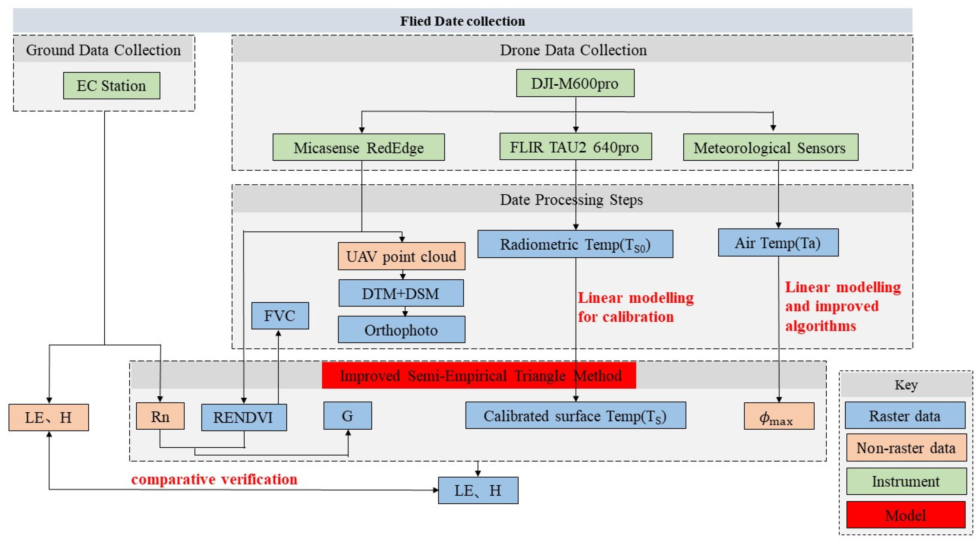
H values were compared with the measured values, and the error was calculated to assess the accuracy. A flow chart of the research process is presented in
Figure 1.
2.1. Test Equipment and Process
2.1.1. Study Area and Test Procedure
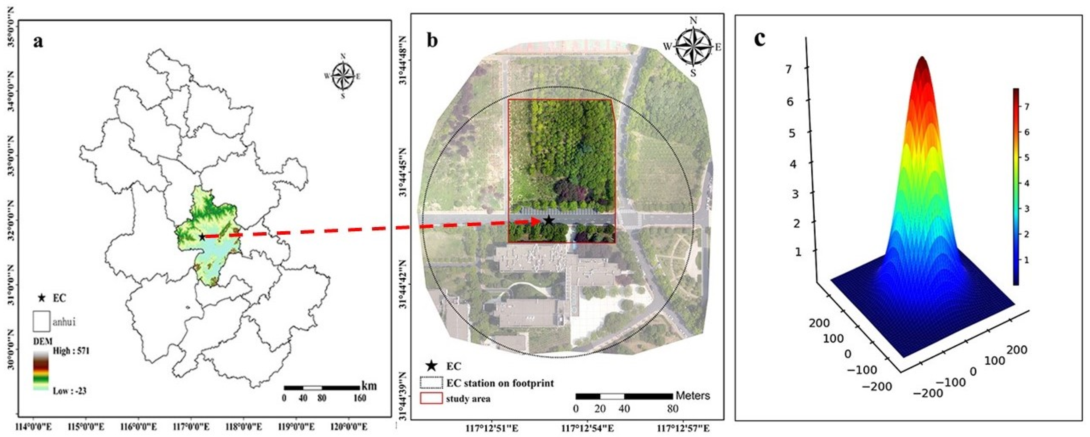
This study conducted experiments at Anhui Jianzhu University in Hefei City, Anhui Province, China, using the combined EC observation system and the UAV observation system. The test location is shown in
Figure 2a,b, with an average tree height of 11 m (relative height) and an average age ranging from 15 to 20 years.
On 28 July 2022, the UAV conducted seven sets of aerial surveys at 9:30, 12:30, 14:30, 15:30, 17:00, 18:30, and 19:30. Each mission lasted 6′28″, with a flight speed of 5 m/s. The weather conditions during the flights were predominantly sunny or sunny/cloudy. The flights were locked to the full 30 min interval of the EC observation system, with an imaging time interval of 1 s. The UAV-captured images were acquired at a relative altitude of 100 m. The UAV carried a multispectral camera (Micasense RedEdge Inc., Seattle, WA, USA) and a thermal infrared camera (FLIR TAU2 R640, FLIR Systems, OR, Wilsonville, USA), both with a maximum trigger rate of 1 Hz. The UAV images covered an aerial survey area of 5.5311 hectares with a 75% overlap. For turbulent heat flux inversion, a specific area of 1.04 hectares was used. An industrial surface temperature thermometer gun (ZTW0503B, CHINT Group Co., Ltd., Wenzhou, China) was used to measure typical surface temperatures, and GPS was used to locate calibration points.
2.1.2. Eddy Covariance (EC) System
The eddy covariance system was used to observe the turbulent heat fluxes within the footprint, and these were used as the actual measured values to validate the results of the UAV estimation. The extent of turbulent heat flux estimation from the UAV data is a fraction of the EC flux footprint, as shown in
Figure 2b. The system consists of a three-dimensional ultrasonic anemometer (CSAT3B), an open-circuit infrared gas analyzer (LI-7500A), a temperature and humidity sensor (U23-001), and a four-component radiometer (CNR4). All instruments operate at a sampling frequency of 10 Hz. For detailed performance parameters of each instrument in the EC observation system, please see
Table 1. The observation system was installed at the top of the observation tower, which stands at a height of 26.1 m.
The range of the EC footprint depends on several factors, such as observation altitude, wind direction and speed, ground roughness, and atmospheric stability (z/L) [
33]. Flux data were computed at 30 min intervals. The radius
of the source area, centered on the location of the measuring instrument, can be calculated using the model proposed by Schmid et al. [
34] as follows:
where
is the measurement height, and
is the observation coefficient, i.e., the contribution of the source area extent to the flux observations.
For this test, the radius of 80% of the radiation source area was calculated to be approximately 114 m based on the installation height of the observation instruments and Equation (1). The effective radiation range is illustrated in
Figure 2b,c.
The raw data were processed using Eddy-pro v7.0.9 to execute optional data correction steps, including peak cutting, coordinate rotation, density correction, and spectral correction. The recorded data were then saved in the GHG format. Eddy-pro also offers various options for data quality control and evaluation, ultimately providing complete flux data. For outlier rejection, the threshold was set at 3.5 times the time-averaged standard deviation through peak-cutting correction. The tilt correction was performed using Wilczak’s quadratic rotation method [
35], and the maximum covariance method was used to determine the time delay between instruments. A 30 min averaging period was used to calculate the fluxes, following current data processing methods for most EC flux observations.
An important prerequisite for vorticity correlation calculations is that most of the vertical transport is achieved by eddy motion, indicating a fully turbulent flow. However, at low wind speeds and stable atmospheric stratification, turbulence tends to be underdeveloped. Under these conditions, the flow is not in a steady state; instead, convection, stagnant flow, and flow divergence may dominate, failing to meet the basic requirements for vorticity correlation measurements. Therefore, the elimination of inappropriate data is crucial for the quality control of flux data. In this study, we used the steady-state test proposed by Aubinet et al. to examine the data [
36]. During the test period, 62.5% of the flux data had a flux variance of less than 30%, meeting the criteria for steady-state conditions. A further 27.08% of the flux data had a flux variance between 30% and 60%, which was considered acceptable. However, 10.42% of the flux data with a flux variance greater than 60% had to be excluded.
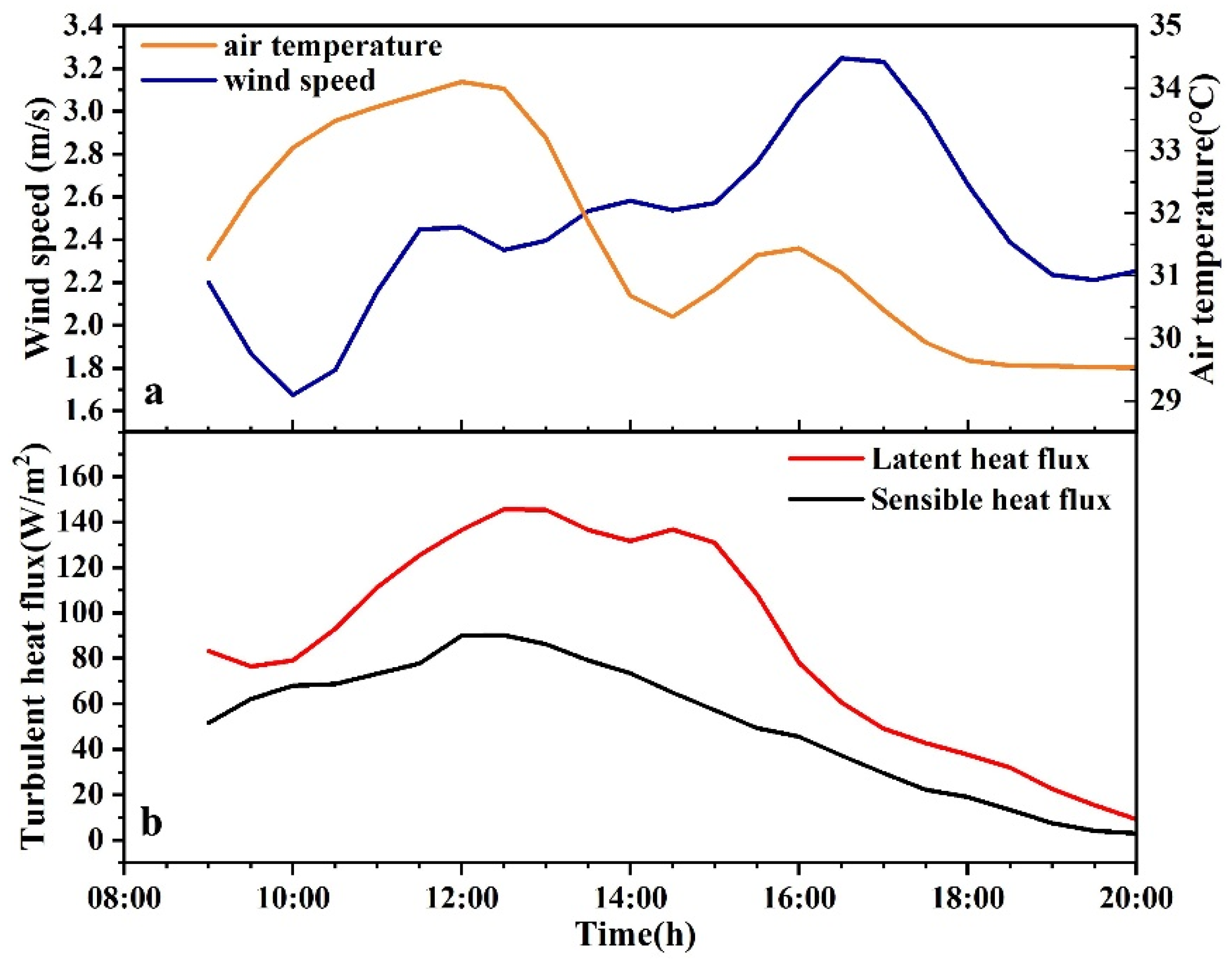
The wind speed was low on the day of the test, as shown in
Figure 3a. The measured data show that both
LE and
H peak around midday, followed by a rapid decrease in turbulent heat flux after 15:30, which is consistent with the change in wind speed. Higher wind speeds increase the mixing and convection of heat and water vapor in the air, thereby increasing the rate of heat transfer and resulting in higher
LE and
H. The significant temperature difference between 10:00 and 16:00 led to high heat transfer through conduction and convection per unit area, resulting in a high H. There was also an increase in the saturated vapor pressure difference in water vapor, which increases the latent heat energy. As a result, turbulent heat fluxes were higher during the period when wind speed and temperature differences were higher.
2.1.3. Unmanned Aerial Vehicle (UAV) and Sensors
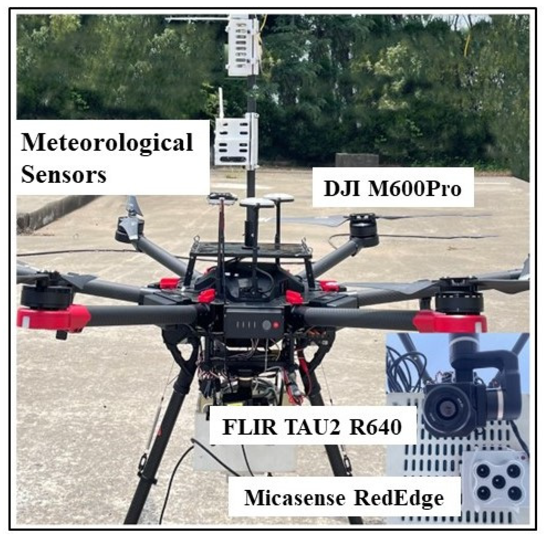
A DJI M600 Pro hexacopter UAV (SZ DJI Technology Co., Ltd., Shenzhen, China) was used in this study (
Figure 4). The M600 Pro is a lightweight and flexibly mountable UAV with an average flight time of 20 min, a maximum payload of 6 kg (actual payload depends on wind speed, humidity, and altitude conditions), and a maximum flight speed of 18 m/s in standard flight mode. This UAV takes off and lands vertically and is designed to be flown using the DJI Pilot 2.5 software. This software allows precise and safe horizontal and vertical flight path planning, with the ability to set flight intervals and payload sensor triggers to achieve the desired forward and lateral images. A 2.4 GHz wireless connection was established between the transmitter, the drone, and the ground station.
In this study, two camera sensors, Micasense RedEdge and FLIR TAU2 R640, were used. The RedEdge camera is a five-channel spectral camera with five spectral bands arranged in a 2-1-2 array, covering electromagnetic waves from the visible to the near-infrared. The bands are arranged in a “Z” shape from the top left to the bottom right: blue, near-infrared, red (mid), green, and red edge.
Table 2 displays the parameters of the RedEdge camera. To obtain accurate images, the RedEdge camera was used to image the original calibration panel (whiteboard) with known spectral albedo values before each flight. These images were then used as calibration input in the calibration process to calibrate the RedEdge images.
The thermal infrared sensor (FLIR TAU2 R640) is equipped with a built-in temperature calculation program. This program uses an atmospheric transport model to calculate atmospheric absorption and scattering of infrared radiation for atmospheric correction. Surface reflectivity correction is achieved by obtaining thermal image data from reference objects with different reflectance values and calculating the corresponding brightness values. Finally, the emissivity of each object’s surface is determined using a gray-body radiation model to calculate the temperature information at the object’s surface.
To ensure consistency in the spatial resolution of the multispectral and thermal infrared imagery, we resampled the multispectral imagery to a spatial resolution of 0.13 m in ArcGIS using the bilinear resampling method. The bilinear resampling method is the product of two linear functions, and the result is independent of the order of interpolation. This method is widely used in the field of image processing [
37].
2.2. Multispectral Data Processing and RENDVI Extraction
To convert the raw DN values of the images into actual measurements, the multispectral camera was first calibrated using the RedEdge camera’s down-light sensor (DLS2, Micasense), which provides multispectral calibration information under changing light conditions. The RedEdge calibration panel was photographed before or after each flight at an altitude of approximately 1 m, ensuring that there were no shadows on the panel. The albedo value of the calibration panel, which represents the proportion of incoming radiation that is reflected by the incident surface but not absorbed, was precalculated by the camera manufacturer by interpolating the panel albedo value. This value could be imported directly into the Pix4D Mapper 4.5 software when performing a radiometric calibration. The multispectral imagery of the UAV was radiometrically corrected, orthorectified, and spliced by creating an orthorectified reference and point cloud in the Pix4D Mapper software, and the values of the vegetation index (VI) were calculated using a band calculator. To reduce the saturation effect of NDVI caused by the near-infrared band of the multispectral camera on the forest canopy and to better capture vegetation changes at a given elevation, this study also used the method proposed by Philip Marzahn. This method uses the red-edge band to calculate the vegetation index, replacing
NDVI with
RENDVI [
32]. The distribution of
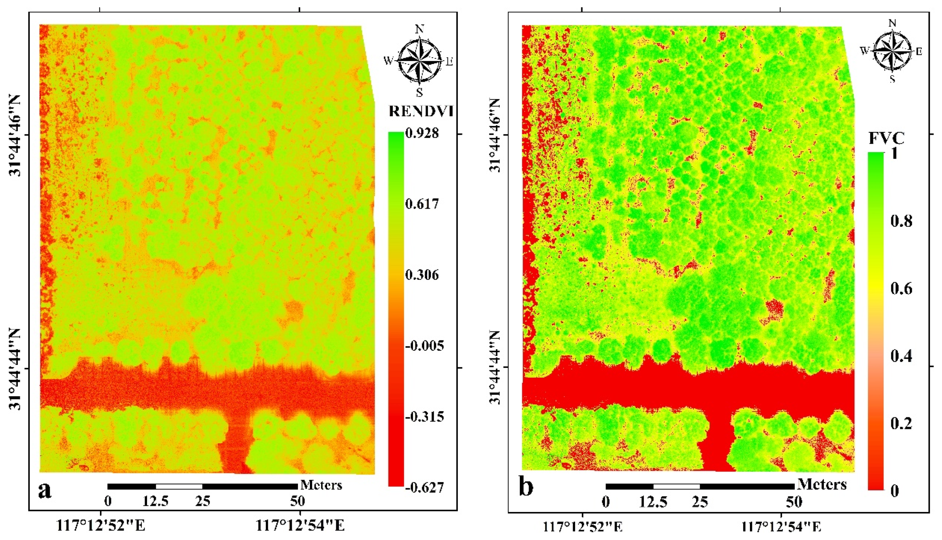
RENDVI in the study area is shown in
Figure 5a.
To improve the positioning accuracy of the images, this study used GNSS (Southern N80T) to measure six full ground control points in the field for position calibration. The average horizontal error was 0.5 m, and the average vertical accuracy was 0.54 m.
RENDVI is an index used to assess the condition of vegetation. As parametric information for estimating heat fluxes using the semi-empirical triangle method in this study, fraction vegetation coverage (
FVC) can better express the spatial distribution and quantification of vegetation on the surface, providing more intuitive and interpretable information that can help analyze spatial changes in vegetation and ecosystem processes. The
FVC is calculated from the RENDVI correlation, as shown in
Figure 5b, using the following equation:
where
RENDVI0 represents the
RENDVI value for bare soil or unvegetated areas with a cumulative percentage of 5%, and
RENDVIS represents the
RENDVI value for fully vegetated areas with a cumulative percentage of 95%.
Within the study area, RENDVI ranged from −0.627 to 0.928, and the average value was 0.413. Most of the values (62.82%) fell between 0.4 and 0.7. The vegetation cover was classified as low (FVC < 0.4), medium (0.4 ≤ FVC ≤ 0.6), high (0.6 ≤ FVC ≤ 0.8), and very high (0.8 ≤ FVC ≤ 1). According to the statistics, the percentages were as follows: 12.02%, 32.59%, 22.01%, and 33.38%, respectively, for areas with low, medium, high, and very high vegetation cover. Overall, areas with medium and high vegetation cover accounted for 87.98% of the total area.
2.3. Processing Thermal Imager Data and Correcting Surface Temperatures
The data captured by FLIR TAU2 R640 were preliminarily calibrated to convert
DN values to surface temperature values (°C) using a simple linear relationship. Equation (4) describes the conversion of
DN to °C. Since the FLIR camera acquires 14-bit data, it is necessary to convert the image data to 16-bit.
Typically, the height of the atmospheric column between the forest canopy and the UAV was 100 m above the forest canopy. The narrow atmospheric column minimized the effects of scattering and absorption by atmospheric gases and aerosols between the radiation reflected from the surface and that measured by the sensor, and the UAV flight time was short enough that no changes in air temperature were observed during the simultaneous in situ measurements. Therefore, no atmospheric corrections were applied to the thermal infrared data in this study.
As surface temperature plays a crucial role in flux estimation and significantly influences the results, the hot and cold spot correction method was applied during the implementation of the original triangle method to improve the surface temperature values obtained from the TAU2 R640 inversion. The aim was to improve the accuracy of LE and H estimates while reducing systematic errors due to external factors such as equipment and radiation. The hot and cold spot correction method is based on measurements at representative “extreme cold spots” (areas with the highest vegetation cover and lowest surface temperature) and “extreme hot spots” (areas with the lowest vegetation cover and highest surface temperature) [
38,
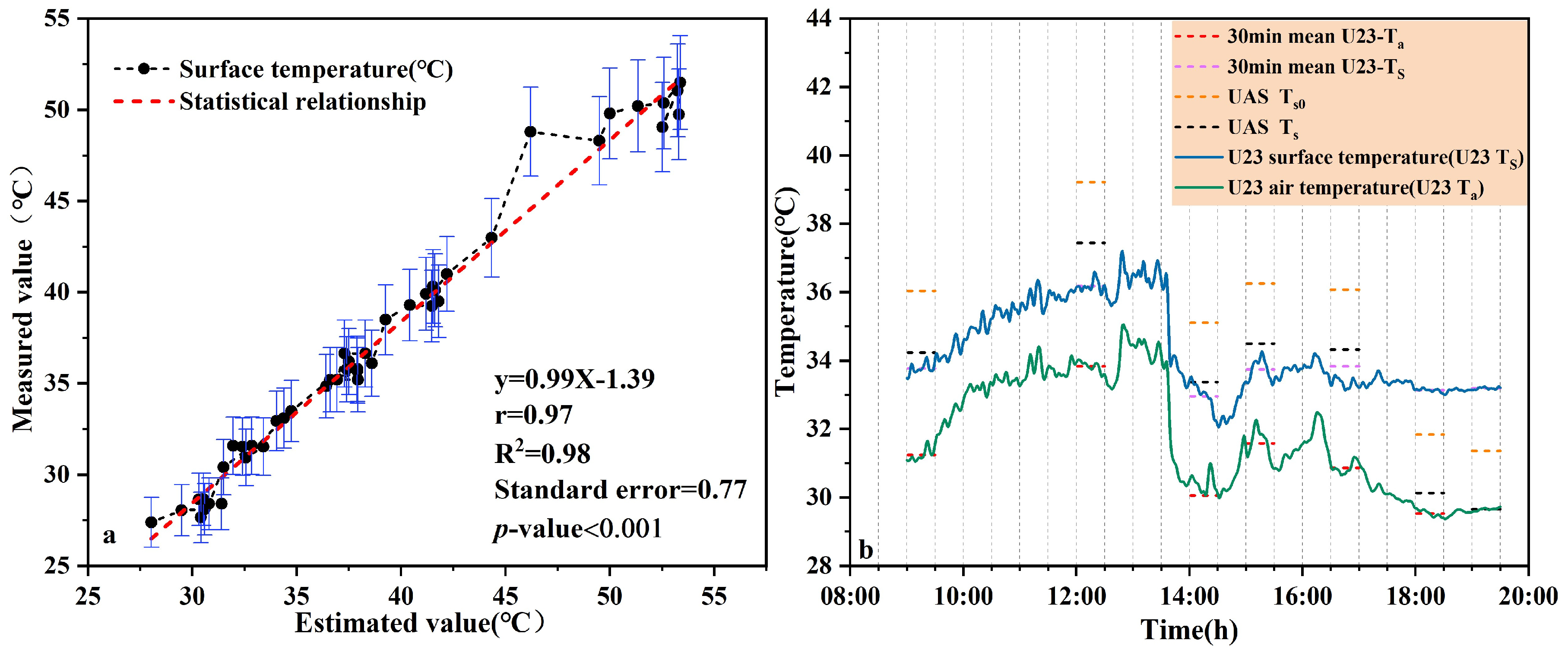
39]. These measurements are corrected by establishing a linear relationship between the measured and inverted temperature values. In this study, an industrial hand-held thermal infrared pyrometer (ZTW0503B) was used to calibrate representative locations before and after each flight to establish their correlation, as shown in
Figure 6.
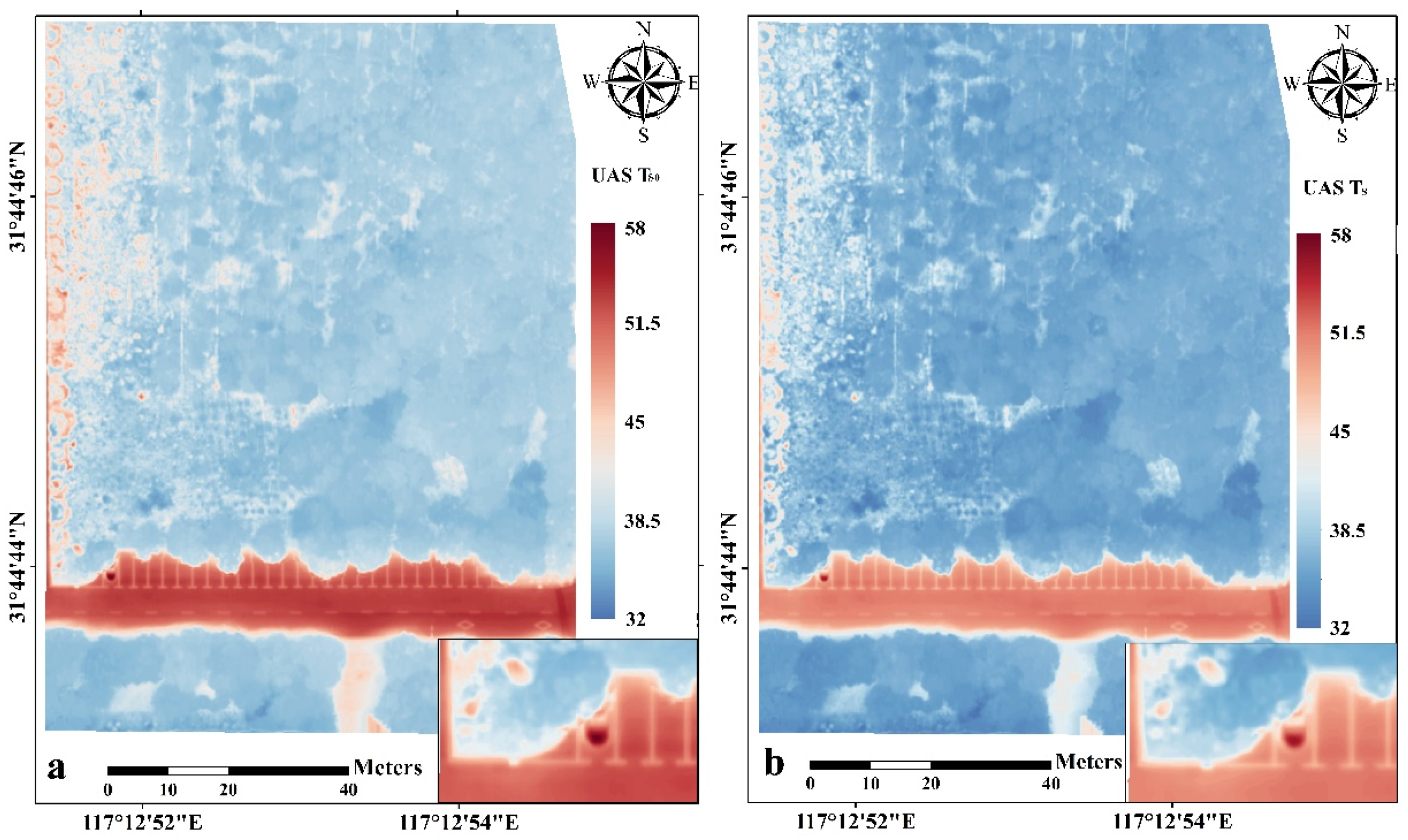
The surface temperatures obtained from FLIR TAU2 R640 inversion were calibrated according to the linear relationship fitted in
Figure 6. The standard error was 0.77 °C with an r of 0.97, and the results of the spatial distribution before and after calibration are illustrated in
Figure 7. These results indicate that the calibration method is suitable for calibrating surface temperatures. The pre-calibration temperatures ranged from 33.76 °C to 57.91 °C, with a mean value of 39.22 °C, while the post-calibration temperatures ranged from 32.03 °C to 55.94 °C, with a mean value of 37.43 °C.
2.4. Research Methods
2.4.1. Semi-Empirical Triangle Method
The semi-empirical triangle method, a remote sensing method that is based on surface temperature and vegetation index (
Ts−
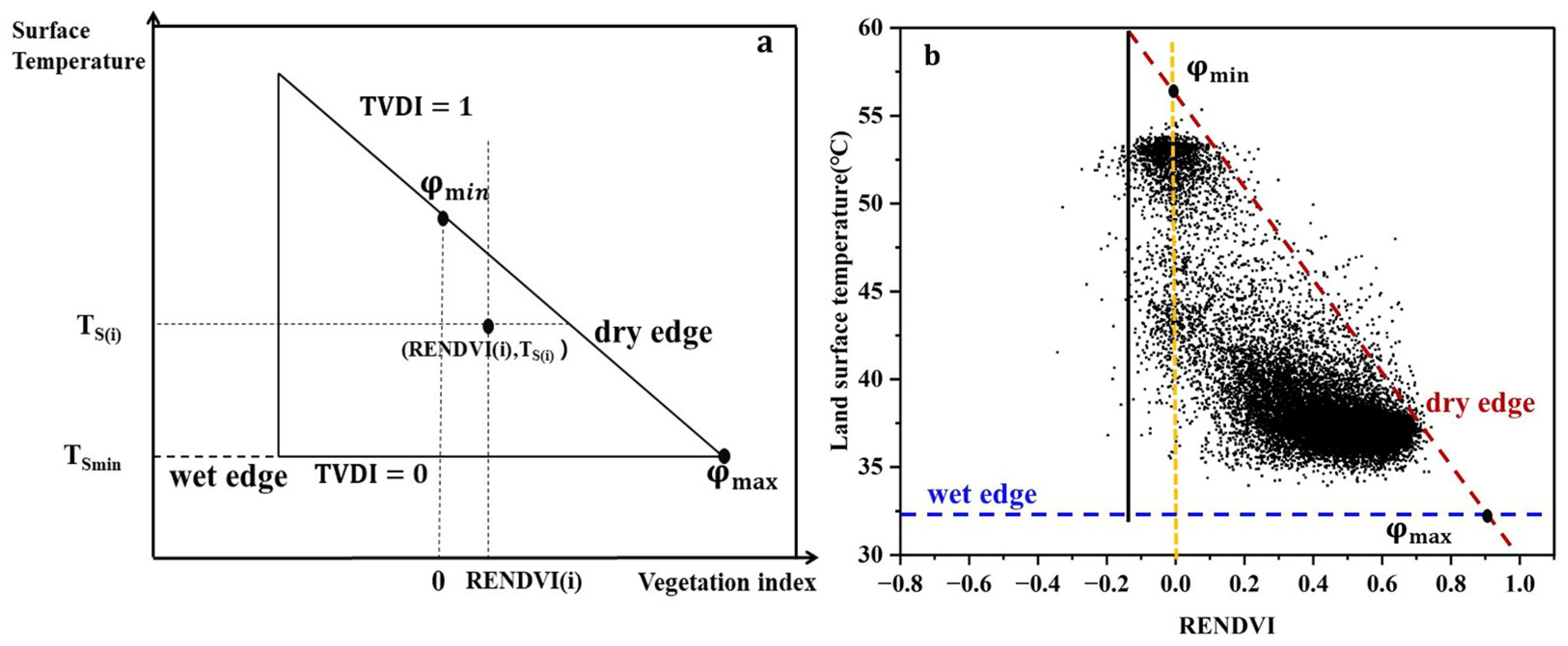
VI) and independent of ancillary data, was used to estimate evapotranspiration and soil moisture. Several studies have reported a triangular shape in the scatter plot of remotely detected T
S versus NDVI, as shown in
Figure 8. The vertical coordinate “
TS” in
Figure 8a represents the radiant surface temperature obtained from the thermal infrared band, while the horizontal coordinate represents the normalized difference vegetation index, commonly abbreviated as
NDVI. However, due to the approximation of the measured area as a homogeneous surface,
NDVI cannot represent the subtle spatial differences in the greenness of vegetation. According to Sims and Gamon [
40], the observation of heterogeneity is the main requirement of the triangle method. Therefore,
RENDVI was used instead of
NDVI.
Two important boundaries in the triangle method are the wet/cold edge at the lower boundary and the dry/warm edge at the upper boundary. When
RENDVI is a constant value, a lower T
S and wet soil were considered a wet edge, representing potential evapotranspiration, while a higher
TS and drier soil were considered a dry edge, representing a limiting condition for soil moisture evapotranspiration. It can also be expressed by the temperature vegetation dryness index (
TVDI) [
41]:
TVDI = (
TSmax −
TS)/(
TSmax −
TSmin).
TVDI takes values between 0 and 1, with higher values indicating proximity to the dry edge. The dry edge and the wet edge intersect at
NDVImax. As shown in
Figure 8a, maximum transpiration occurs when the dry edge intersects the maximum value of
NDVI, and minimum transpiration occurs when the dry edge intersects the
NDVI at 0, with
TVDI being 0 at
Tsmin, and 1 at
Tsmax. The
RENDVI and
TS pixel values are clustered on the right side of the triangle formed by the wet and dry edges, as shown in
Figure 8b. Theoretically, it could be argued that the temperature axis of the
TS−
RENDVI scattering should represent the airspace temperature gradient (
TS −
Ta); due to data availability reasons, (
TS −
Ta) is often replaced by T
S in remote sensing applications [
42]. The advantage of this method is that it uses the surface radiation temperature instead of the aerodynamic temperature. It links the heat flux to the difference between the surface radiation temperature and the air temperature through the aerodynamic impedance.
The
TS−
VI semi-empirical triangle method was developed from the Penman–Monteith equation. The calculation process is based on the energy balance equation (Equation (5)), and the core of the calculation involves parameterizing
in the Priestley–Taylor equation. This is achieved by replacing the resistance term of the Penman–Monteith equation with a parametric representation of
in the air power term. The goal is to obtain a simplified form of the predicted LE [
8,
43]. The equation for energy balance can be expressed in the form of Equation (6):
where
is a dimensionless dynamic coefficient, representing the effective surface resistance to evapotranspiration. It is independent of any single surface attribute [
44].
Rn is the net radiative flux (W/m
2), which exhibits little regional variability on the microscale [
45]. The footprint of EC flux in this study covered the study area, and the mean value of Rn measured by CNR over a half-hour period was used as the parameter to be substituted in Equation (6). G is the soil heat flux, ∆ is the slope of the temperature-saturated water–gas pressure curve (Kpa∙°C
−1), and γ is the thermometer constant (Kpa∙°C
−1).
The Priestley–Taylor coefficients for
can be calculated inversely using the distributions of
RENDVI and
TS. The pixel at (
,
) has a
value. The equations are as follows:
where
is the smallest value of
,
which represents the Priestley–Taylor coefficients of pixel i;
and
are the maximum and minimum values of
TS, respectively;
is the
TS value of pixel
i; and Δ/(Δ + γ) is known as the air temperature control coefficient.
G is usually much smaller than
Rn and is closely correlated with it, as well as with
RENDVI;
G is usually about 10–15% of
Rn. Ortega-Farías proposed an equation for estimating
G [
46].
2.4.2. Semi-Empirical Triangle Method with Improved Calculation of
According to Equation (8),
is the
value where the maximum value of RENDVI intersects the wet edge and is related to the air temperature control coefficient Δ/(Δ + γ), which can be expressed in the model of the semi-empirical triangle method using the following equation [
47]:
To simplify the calculation, the following formulae proposed by Richards in 1971 are used [
48]:
The constant γ of the thermometer can be obtained as follows:
where
Ta is the temperature of air (K),
P0 is the standard atmospheric pressure at sea level,
Z is the altitude,
P0 = 1013.15 hpa, and
Cp = 1012 J/kg∙K.
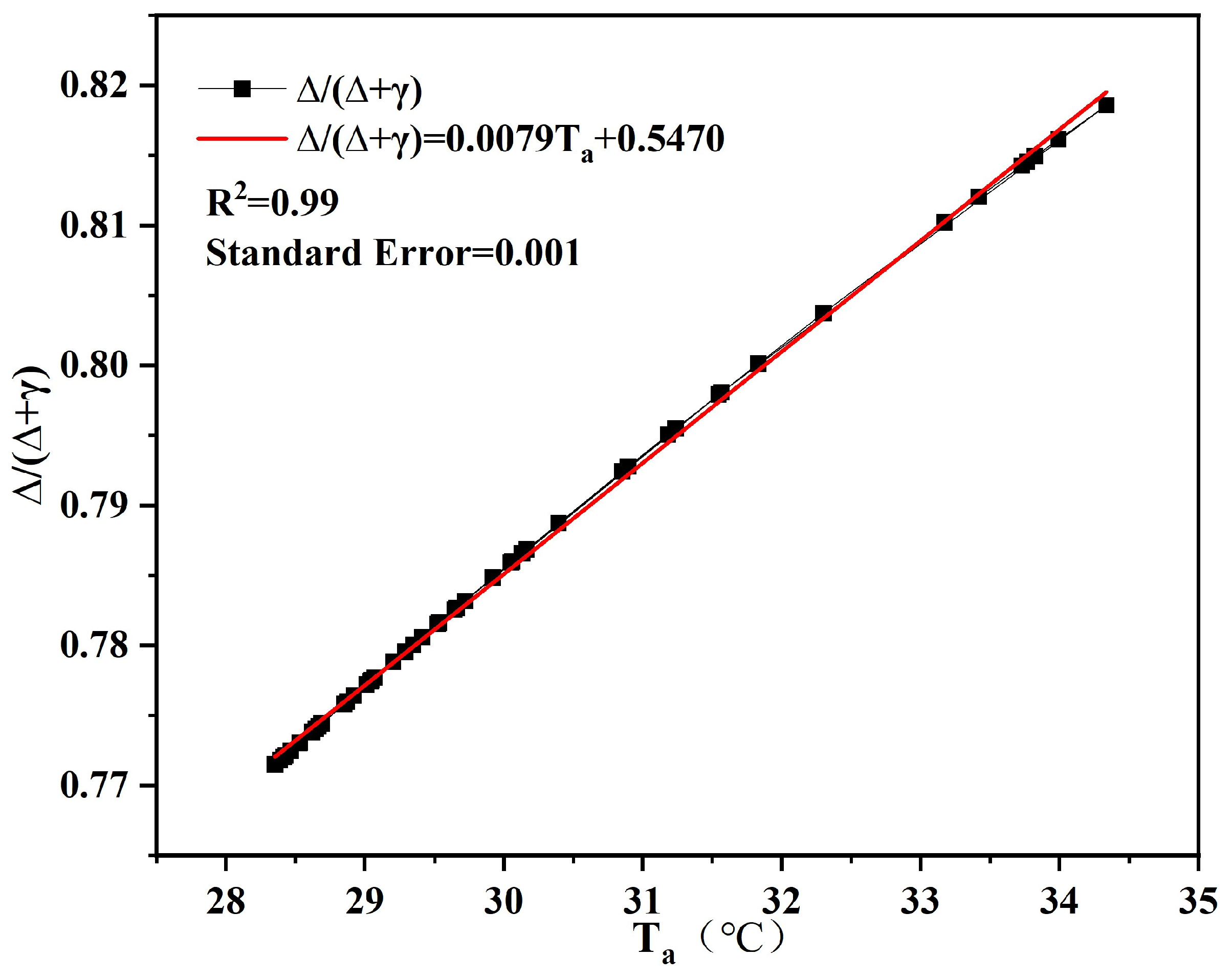
In the estimation of LE and H using UAV-captured data combined with the triangle method, plays a crucial role in the calculation principle, but the calculation process is complex. To simplify the calculation process as much as possible without affecting the accuracy of the estimation, the parameter was refitted based on Equations (11)–(17), and a model was established for the linear relationship between ∆/(∆ + γ) and Ta to improve the calculation process of the parameter and optimize the semi-empirical triangle method for the estimation of turbulent heat fluxes in urban mixed forest areas.
Figure 9 shows the temperature control factor Δ/(Δ + γ) as a function of temperature Ta. Δ/(Δ + γ) increases with increasing temperature, and the results show an excellent fit to the linear model. This model can effectively replace the complicated calculation process, allowing the derivation of a semi-empirical triangle model suitable for estimating turbulent heat fluxes in urban mixed forests based on the improved
calculation process outlined in Equations (18) and (19).
Based on the above method, the
LE and
H at each pixel point in the study area were estimated, and the correlation coefficient (r) and root mean square error (RMSE) were compared with the measured values. The coefficients of determination (R
2) are obtained through energy flux comparisons using uncorrected EC station data (measured) and UAV-derived (estimated) data. The expressions are as follows:
where
denotes the
LE or
H values measured by the EC station at different times;
was the average of several measurements of
;
is the
LE or
H values estimated based on the UAV-collected data at different times using the semi-empirical triangle method;
was the average of several estimates of
; and
N is the number of trials, which is 7 in this study.
3. Results
Pix4D Mapper was used to preprocess the RedEdge and TAU2 R640 data to obtain
RENDVI and T
S. Based on the semi-empirical triangle method, the spatial distribution of
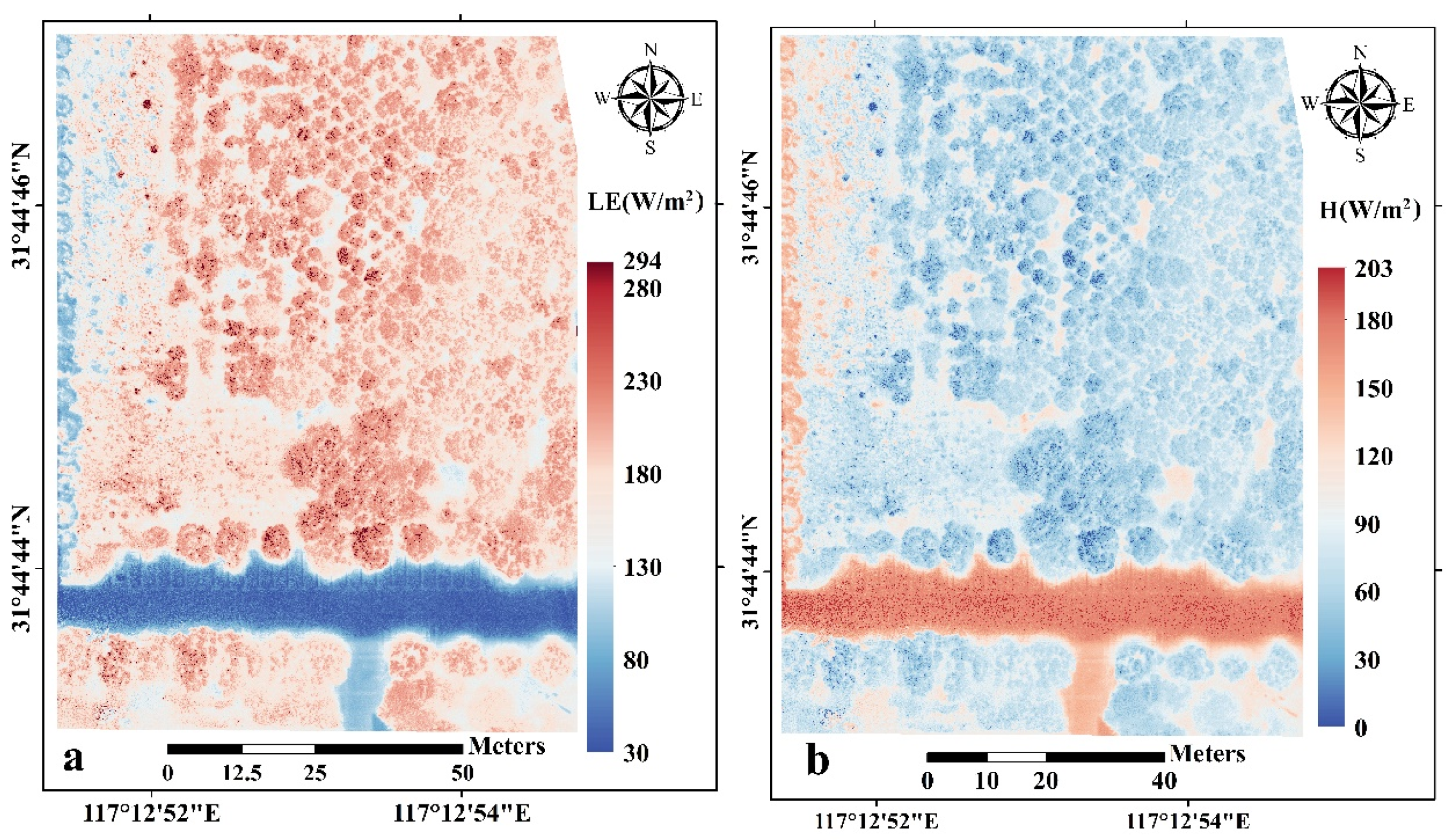
LE in the study area was estimated, as shown in
Figure 10a. The
G values were calculated using Equation (10), and the
H values were estimated based on the principle of energy balance using Equation (5), as shown in
Figure 10b. As can be seen in
Figure 10, the estimation results from the UAV data with a 0.13 m spatial resolution clearly show the turbulent heat fluxes of individual trees or even individual leaves.
LE was lower in open fields, soil patches, and leafless branches and relatively higher in areas with higher vegetation cover; the result is consistent with previous studies examining
LE and
H in other regions [
11,
49]. This indicates that highly vegetated areas show a higher potential for evapotranspiration. Areas with high vegetation cover have relatively low heat transfer, low heat flux, and low
H and are described as cold areas with relatively low radiation. In this study, the
H values were higher in open spaces and patches of ground, which are areas where heat transfer is concentrated, and warm areas with relatively strong radiation.
To verify the accuracy of the turbulent heat flux values estimated from the UAV data, the mean values of
LE and
H at each pixel point in the study area were compared with the actual EC measurements. The results show that the estimated
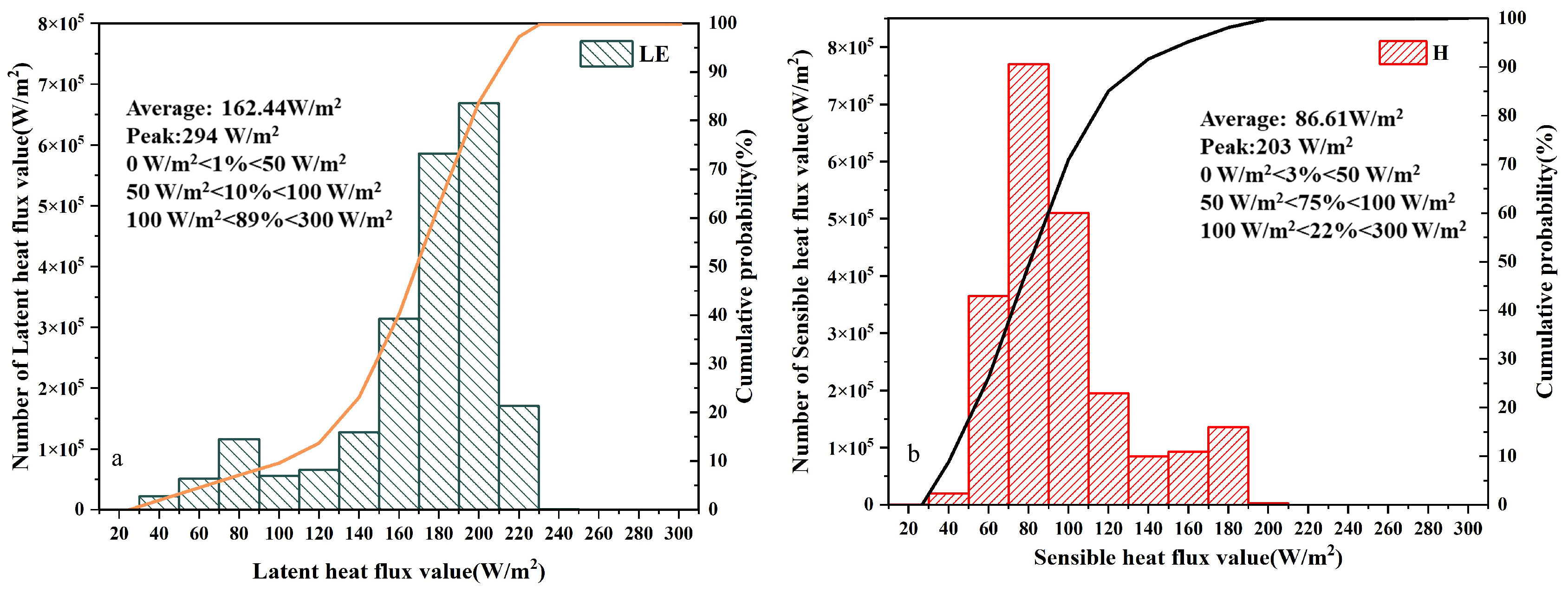
LE during the 12:30 flight period had an average value of 162.44 W/m
2, and the estimated
H had an average value of 86.61 W/m
2 in the study area; the results of the heat flux estimation for each pixel point are shown in
Figure 11. The
LE values were mostly distributed between 100 and 300 W/m
2, accounting for 88.73%, and the
H values were mostly distributed between 50 and 100 W/m
2, accounting for 75.16%. The range of
H values was smaller than that of LE, indicating that the study area has a large vegetation cover. Potential evapotranspiration was high during the day, and most of the area showed a high latent heat status. This is attributed to the predominant vegetation cover in the area, which converts some of the heat flux to latent heat through transpiration, thus reducing
H. Furthermore, the low wind speed on the day of the test resulted in a lower heat exchange rate between the atmosphere and the surface. The test was carried out in summer, with intense solar radiation and prolonged insolation, resulting in more solar energy being absorbed by the surface. Some of the
H was used to heat the surface and was not transferred to the atmosphere. Consequently,
LE was higher than
H during this period.
The LE and H values obtained from the EC observation system during the same time period were 148.08 W/m2 and 80.56 W/m2, respectively. Compared to the semi-empirical triangle estimation results based on the UAV-captured data, the estimated LE values were higher than those observed by the EC observation system, with an absolute difference of 14.36 W/m2 and a relative difference of 9.70%. The estimated H values were higher than the measured values, with an absolute difference of 6.05 W/m2 and a relative difference of 7.50%. As the study area is in the suburban area, LE estimates may be slightly higher as they are influenced by surface temperatures affected by the urban heat island effect, and additional energy balances are included in the H values.
To further analyze the results of the estimation based on UAV-captured data using the semi-empirical triangle method, data from several other flight periods were processed to obtain
LE and
H for different periods within the same day in the study area. These estimates were then compared with the measured fluxes obtained from the EC observation system, as shown in
Figure 12. The deviations of the latent and sensible heat flux estimates from the eddy correlation covariance observations were less than 25 W/m
2 in all seven sets of tests. The maximum deviation of the
LE value was 23.11 W/m
2, and the minimum deviation was 4.43 W/m
2, while the maximum deviation of the
H value was 15.45 W/m
2, and the minimum deviation was 3.42 W/m
2. Considering that an absolute error of <50 W/m
2 is considered desirable [
46], the method is considered reliable for estimating turbulent heat fluxes.
The results of
LE and
H estimated by using the method described in this paper were compared with those estimated by using the traditional triangle method. Correlation coefficients (r) and root mean square errors (RMSE) were used to evaluate the correlation between the estimated and measured values. The r and RMSE values are shown in
Table 3. Both
LE and
H values estimated by the two methods had a high correlation with the measured values. The r between the LE values estimated by the method described in this paper and the measured values was 0.95, which improved by 0.04 when compared to the traditional triangle method, and the RMSE was 35.96 W/m
2; the r of the estimated and measured H values was 0.91, which improved by 0.06 compared to the traditional triangle method, and the RMSE was 9.77 W/m
2.
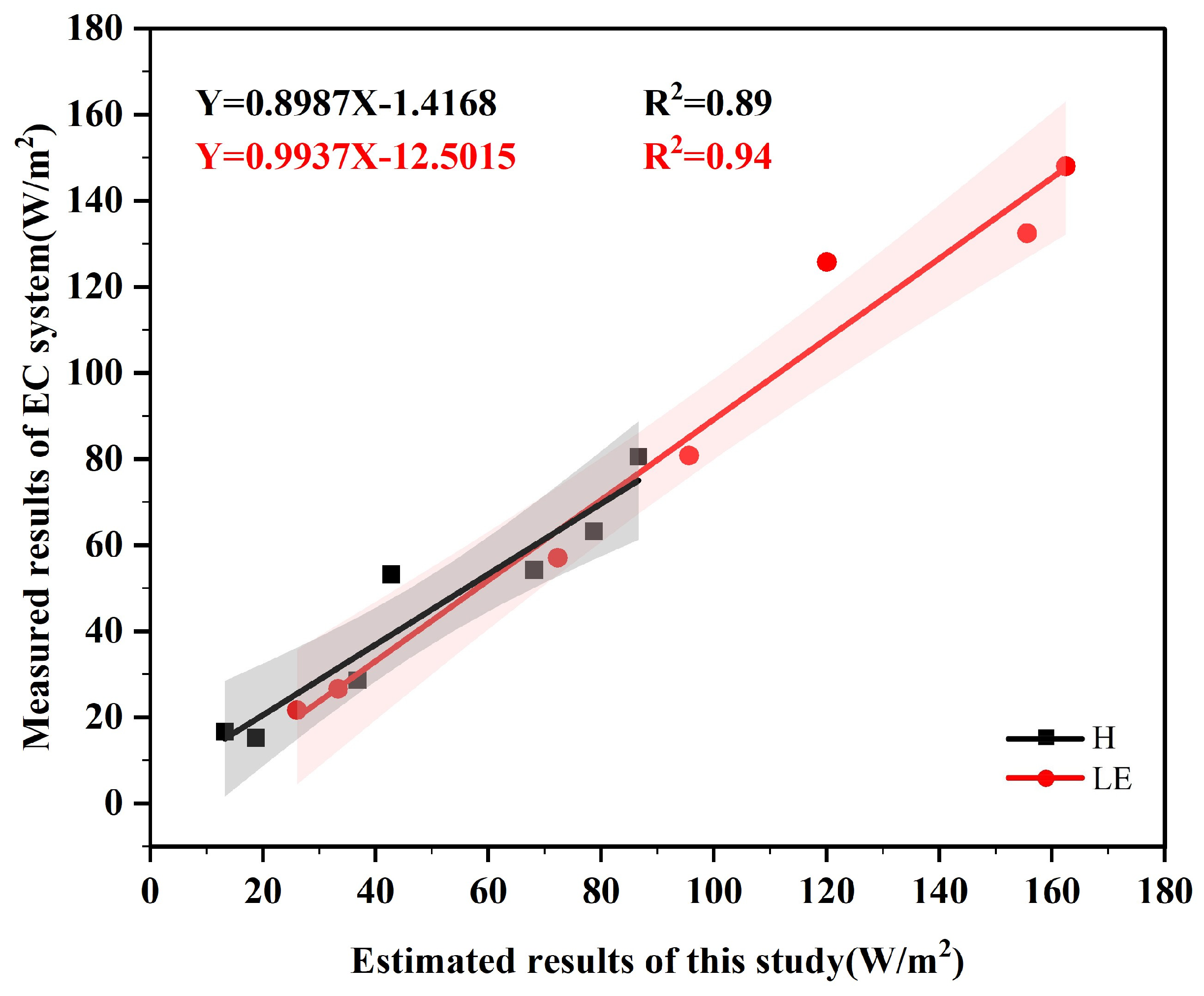
Using the seven sets of estimation results within the study area, a linear relationship model was formulated to show the relationship between the turbulent heat fluxes estimated using the UAV-captured data and the actual measured values at different times of the test. As shown in
Figure 13, the coefficient of determination for the
LE model, R
2, is 0.94, and for the
H model, R
2, is 0.89, confirming that the linear relationship models fitted to the
LE and
H values have a high degree of fit.
4. Discussion
In this study, UAV-based estimates of LE and H were carried out using multispectral and thermal infrared orthomosaics in combination with an improved semi-empirical triangle method over an urban forest on the campus of Anhui Jianzhu University in Anhui Province, China. Compared to the measured data of the EC system, the absolute errors of several groups of estimation results are less than 25 W/m2; the mean value of the absolute error of LE is 10.43 W/m2, while that of H is 4.75 W/m2; and the mean value of the relative error of LE is 16.22%, while that of H is 9.89%. With this approach, LE and H estimates can be traced back to individual trees, allowing the differentiation of leafless branches, dead trees, and lianas. Although the method still needs to be validated with ground-truthing data, it has a progressive role to play in the analysis of individual plant heat fluxes in urban forests, and the results obtained are consistent with the results of satellite estimation.
The estimation process of the traditional triangle method is complex and requires a multitude of parameters. The functions of Δ/(Δ + γ) and Ta were constructed for the study area, and the fitted model has an R
2 of 0.99. We believe that the fitted model explains the variability in the observed data well and, therefore, simplifies the process of calculating
in the triangle model without compromising the accuracy of the estimates. Although this methodology shows improved estimation efficiency, its validation is limited to the spatial scale of the study area. Further validation at different spatial scales is required to ensure the generalizability of the model. To improve the accuracy of the
LE and
H estimates, a calibration procedure was implemented for the surface temperature, a crucial input parameter in the triangle method. The integration of these two extensions resulted in the development of a semi-empirical triangle method tailored to the estimation of LE and H in urban mixed forest environments. Spatial alignment is a critical step in this study. The raw data collected by the UAV do not contain accurate position information, so eight ground control points (GCPs) were established using differential GPS to optimize the position accuracy of the images. To ensure the precise alignment of both multispectral and thermal infrared orthomosaics, a substantial number of ground control points (GCPs) were employed. However, this procedure is time-intensive, and the predominantly forested nature of the study area poses challenges to alignment accuracy due to variations in elevation. Irene Aicardi et al. [
50] explored a novel approach for achieving automated alignment of multitemporal high-spatial-resolution images, eliminating the need for ground control points. The study demonstrated minimal differences between the results obtained through automatic alignment and manual alignment. However, it is important to note that the application of this method to automatically align multispectral and thermal infrared images has not yet been conducted, leaving room for potential exploration in future research endeavors.
The triangle method has been widely utilized for estimating turbulent heat fluxes and has shown good agreement with measured values in several studies. However, it relies on simplified assumptions, including steady-state conditions and uniform surface moisture distribution, which may not hold true in complex terrain and highly urbanized areas. These factors can potentially affect the accuracy of estimation results. Moreover, the applicability of this method can vary across different climatic conditions, geographical settings, and scales, necessitating further validation and adaptation. Additionally, the temporal resolution of the semi-empirical triangle method typically assumes temporal and spatial averaging, disregarding short-term variations. Consequently, it fails to capture instantaneous changes in latent and sensible heat fluxes. Nevertheless, when combined with UAV data, the proposed semi-empirical triangle method offers a more flexible approach for estimating near-surface turbulent heat fluxes.
Looking forward, the applied and tested method allows the integration of the UAV system in a multi-data analysis approach. Thus, the method is complementary to gaps at different temporal and spatial resolutions and can also be used to validate LE and H based on the inversion of remote sensing data at different scales. Compared to LE and H estimated from coarse-resolution remote sensing products (e.g., MODIS 500 m × 500 m resolution), the UAV-based method provides more detail, as can be seen in
Figure 10. In addition, our approach allows the calculation of refractive index structure constants (
) associated with optical turbulence intensity in the near-surface atmosphere based on the estimated turbulent heat flux. This method provides a novel predictive avenue in situations where direct measurement of
is not feasible, and it has some scientific value.
5. Conclusions
In this research, turbulent heat flux was estimated at a high spatial resolution of 0.13 m. In areas characterized by open space and low vegetation cover, latent heat flux (LE) was found to be lower, while sensible heat flux (H) was higher due to intensified radiation and concentrated heat transfer. On the contrary, forested areas with dense vegetation cover exhibited a high potential for evapotranspiration, resulting in an elevated LE, while H was lower due to the cooler nature of such land types. The study area exhibited extensive vegetation cover, with a predominant occurrence of high latent heat conditions during the daytime. Consequently, LE values consistently exceeded H values. This behavior is mainly attributed to the dense vegetation cover, which reduces surface–atmosphere heat exchange, while open spaces contribute to higher sensible heat areas.
To validate the accuracy of the UAV estimation, a comparison was made with the results obtained from an analysis of data from the EC system, which was carried out simultaneously. The findings revealed an absolute difference in LE ranging from 4.43 to 23.11 W/m2, with negative values observed specifically at 15:30. For H, the maximum deviation was 15.45 W/m2, while the minimum deviation was 3.42 W/m2, with negative values also recorded at 15:30. The correlation analysis between the estimated and measured result values demonstrated a strong relationship for LE, with a correlation coefficient (r) of 0.95 and a root mean square error (RMSE) of 35.96 W/m2. Similarly, for H, the correlation coefficient was 0.91 with an RMSE of 9.77 W/m2, indicating a robust correlation between the estimated fluxes and the measured values. The improved calculation process of the semi-empirical triangle method led to a 0.04 improvement in LE correlations and a 0.06 improvement in H correlations compared to the traditional approach. Therefore, the semi-empirical triangle method incorporating these improvements exhibits enhanced accuracy in estimating turbulent heat fluxes.
The
TS-RENDVI triangle method is used in a nonuniform surface environment to better account for surface heterogeneity and provide more accurate estimation results [
27]. The study area consists of an urban mixed forest, which fulfills the conditions required for the triangle method. Although there are some differences between the estimated values and the measured values, the overall correlation is high, and the errors are minimal. Consequently, the estimation of turbulent heat fluxes in urban mixed forests using the UAS semi-empirical triangle method provides a flexible and high spatial resolution approach for turbulent heat flux estimation that complements the EC system analysis method.
