Article

A New Combination Approach for Gibbs Phenomenon Suppression in Regional Validation of Global Gravity Field Model: A Case Study in North China

1
School of Geospatial Engineering and Science, Sun Yat-sen University, Zhuhai 519082, China
2
Key Laboratory of Comprehensive Observation of Polar Environment, Sun Yat-sen University, Ministry of Education, Zhuhai 519082, China
3
Innovation Academy for Precision Measurement Science and Technology, CAS, Wuhan 430071, China
*
Author to whom correspondence should be addressed.
Remote Sens. 2024, 16(15), 2756; https://doi.org/10.3390/rs16152756
Submission received: 10 July 2024 / Revised: 25 July 2024 / Accepted: 26 July 2024 / Published: 28 July 2024

Abstract

:
A global gravity field model (GGM) is essential to be validated with ground-based or airborne observational data for the accurate application of the GGM at a regional scale. Furthermore, accurately understanding the commission errors between the GGM and observational data are crucial for improving regional gravity fields. Taking the North China region as an example, to circumvent the omission errors, it is necessary to unify the spatial resolutions of the EIGEN-6C4 model and terrestrial gravity observational data to 110 km (determined by the distribution of gravity stations) by employing the spherical harmonic function for the EIGEN-6C4 model and the Slepian basis function for the gravity data, respectively. However, the application of spherical harmonic function expansions in the gravity model results in the Gibbs phenomenon, which may be a primary factor contributing to commission errors and impedes the accurate validation of the EIGEN-6C4 model with terrestrial gravity data. To effectively mitigate this issue, this study proposes a combination approach of window function filtering and regional eigenvalue constraint (based on the Slepian basis). Utilizing the EIGEN-6C4 gravity model to derive the gravity disturbance field at a resolution of 110 km (with spherical harmonic expansion up to the 180th degree and order), the combination approach effectively suppresses over 90% of high-degree (above the 120th degree) Gibbs phenomena. This approach also reduces signal leakage outside the region, thus enhancing the spatial accuracy of the regional gravity disturbance field. A subsequent comparison of the regional gravity disturbance field derived from the true model and terrestrial gravity data in North China indicates excellent consistency, with a root mean squared error (RMSE) of 0.80 mGal. This validation confirms that the combined approach of window function filtering and regional eigenvalue constraints effectively mitigates the Gibbs phenomenon and yields precise regional gravity fields. This approach is anticipated to significantly benefit scientific applications such as improving the accuracy of regional elevation benchmarks and accurately inverting the Earth’s internal structure.

1. Introduction

The International Centre for Global Earth Modelling (ICGEM) has recently released a suite of ultra-high-degree global gravity field models (GGMs), including EGM2008 [1], EIGEN-6C4 [2], SGG-UGM-2 [3], and XGM2019e [4] on the website http://icgem.gfz-potsdam.de/home, accessed on 10 July 2024. Utilizing long-term observations from satellite gravity missions and high-precision and high-resolution gravity anomaly datasets, these models provide significantly enhanced accuracy and resolution compared to their predecessors, such as EGM96 [5] and EIGEN-CG01C [6]. These advances make them invaluable for various applications, including the unification of elevation benchmarks, precision satellite orbit determination, dynamic sea surface topography calculations, studying the Earth’s internal tectonics, etc.
Significant differences exist in the precision of the above GGM across various regions, particularly in areas lacking ground-based and airborne-based observational data. To accurately apply the GGM on a regional scale, it is essential to validate it using observational data (e.g., terrestrial gravity, GPS/leveling, or airborne gravity). Numerous studies have analyzed the discrepancies between the GGM and observational data in regions such as South America, Europe, Australia, and Africa [7,8,9,10,11,12,13,14,15]. These studies indicate that the regional differences between the GGM and observational data are primarily classified as omission and commission errors. The omission errors in the GGM with observational data can be corrected by ultra-high-degree residual terrain model (RTM) data or circumvented by unifying the spatial resolution of the model and observational data. In contrast to omission errors, commission errors are difficult to model at a regional scale, and their accurate identification is crucial for accurately applying the GGM to regional gravity fields.
Recently, there has been limited research on commission errors of the GGM with observational data in the Chinese region. Furthermore, we have collected terrestrial gravity observational data with a spatial resolution of approximately 110 km in North China. Given the highest accuracy of the EIGEN-6C4 model in the Chinese context [3,16], we plan to use this model along with terrestrial gravity observational data for comparative validation in the North China region.
Given that residual terrain model (RTM) data are not fully representative of full-spectrum terrain undulations and that terrain density is diverse, correcting for omission errors may introduce some uncertainty [10,17,18]. Consequently, unifying the spatial resolution between the model and observational data is more appropriate for studying commission errors at a regional scale. In North China, the EIGEN-6C4 model can derive a regional gravity disturbance field with a spatial resolution of 110 km through spherical harmonic function expansion. However, due to the sparse and irregular distribution of terrestrial gravity observational data, obtaining a regional gravity disturbance field with a spatial resolution of 110 km is challenging. Slepian basis functions, which can equivalently transform to spherical harmonic functions and are unaffected by the irregular distribution of stations [19,20,21], are widely used in GNSS deformations or ground gravity changes for obtaining time-varying regional gravity fields [22,23,24]. Therefore, for the terrestrial gravity data in the North China region, the Slepian basis function can be utilized to achieve a terrestrial gravity data-based regional gravity disturbance field (TGD-RGDF) with a spatial resolution of 110 km.
However, when the GGM is expanded into the spatial domain using spherical harmonic functions, the Gibbs phenomenon occurs, resulting in ringing effects and signal distortions [25], introducing an error that may approximate 9% of signals [26], and manifesting as elevation and gravity disturbances with magnitudes reaching tens of cm and mGal level, respectively. The Gibbs phenomenon may be a primary factor contributing to commission errors, undermining the accuracy of verification and application of the GGM on a regional scale. To mitigate the Gibbs phenomenon associated with spherical harmonic functions, various window functions, such as Hanning, Lanczos, and Gaussian windows, are widely employed [7,27]. Although these methods generally yield satisfactory results on a global scale, they may result in signal contamination within regional gravity fields due to external leakage. To address the impact of external leakage, this study proposes a mitigation method that converts the spherical harmonic functions to the Slepian basis functions and introduces constraints based on the regional eigenvalue of the Slepian basis.
Therefore, in this study, a combination approach of window function filtering and regional eigenvalue constraint is proposed to refrain the Gibbs phenomenon in the regional gravity field, and the ‘true’ model regional gravity disturbance field (TM-RGDF) with the Gibbs phenomenon suppressed from the EIGEN-6C4 model is compared and validated with the TGD-RGDF derived from terrestrial gravity data in North China. The brief process is as follows: Firstly, the spherical harmonic coefficients of the EIGEN-6C4 model are filtered using the Hanning window. Subsequently, the filtered coefficients are transformed into Slepian basis coefficients for introducing regional eigenvalue constraints to obtain the TM-RGDF with a spatial resolution of 110 km in North China. Then, the TGD-RGDF from terrestrial gravity data is constructed based on Slepian basis functions in North China. Finally, the TM-RGDF is compared and validated with the TGD-RGDF. This approach can effectively mitigate the Gibbs phenomenon and achieve a high-precision regional gravity field, which is crucial for precisely unifying regional elevation benchmarks, accurately determining the Moho discontinuity in the region, etc.

2. Methodology

2.1. Calculate the Regional Gravity Disturbance Field Based on the Global Gravity Field Model

The Earth’s gravity field model is represented by a series of truncated to Nth degree and order (d/o) gravitational potential spherical harmonic functions, as follows:
V H , θ , λ = G M R + H n = 2 N R R + H n m = n n υ ¯ n , m Y ¯ n , m θ , λ
where G and M stand for the Earth’s gravitational constant and the Earth’s mass, respectively; R and H indicate reference radius and altitude above the reference sphere, respectively; θ   and λ are colatitude and longitude, respectively; Y ¯ n , m are the fully normalized surface spherical harmonics of gravitation; υ ¯ n , m are the spherical harmonic coefficients of gravitation; n and m denote the degree and order, and N is the maximum degree of truncation. The formula for resolving gravity disturbances using the EIGEN-6C4 gravity field model, derived from the series expansion of spherical harmonic functions, is as follows:
δ g H , θ , λ = n = 2 N m = n n g n , m Y ¯ n , m θ , λ g n , m = G M R + H 2 · n + 1 · R R + H n · υ ¯ n , m
where δ g indicates gravity disturbances; g n , m are the surface spherical harmonic coefficients of gravity disturbance.

2.2. Refrain Gibbs Phenomenon Using Window Function and Regional Eigenvalue Constraint

The gravity disturbance field, expanded by spherical harmonic functions, exhibits the Gibbs phenomenon. Various window functions have proven effective in mitigating the Gibbs phenomenon at high degrees of spherical harmonic expansion and show similar efficacy when applied to the spherical harmonic coefficients of Earth’s gravity field model. In this study, we utilize the widely employed Hanning window to filter the spherical harmonic coefficients of Earth’s gravity field model. The filtering is performed according to the following formula in the spherical harmonic domain:
g n , m w = W n · g n , m W n = 0.5 · 1 + cos π n N + 1
where W n are the Hanning window functions in the spherical harmonic domain; g n , m w are the gravity disturbance harmonic coefficients after Hanning window filtering used directly in Equation (2) to calculate the gravity disturbance.
With the implementation of window function filtering, external signals will leak into the regional gravity disturbance field. To address this issue, we first introduce the regional Slepian basis functions to convert the spherical harmonic functions of the gravity field equivalently [19,20,21]. In North China, to seek a basis of functions for gravity disturbances whose energy is maximally concentrated within a region, the spatial energy concentration ratio should be maximized as β 2 = δ g 2 d Ω / δ g 2 d Φ m a x , where Ω is the region of North China and Φ is the whole sphere of the Earth. Then the eigen-functions of a Fredholm integral eigenvalue equation in the spatial domain are derived as:
n = 0 N m = n n D n , m , n , m g n , m = β 2 g n , m , D n , m , n , m = Ω Y ¯ n , m Y ¯ n , m d Ω ,
The (N + 1)2 eigenvalues β and eigenvectors f n , m can be obtained by solving the above integral equation. We set N = 180, for 110 km spatial resolution. Using these eigenvectors, the Slepian basis functions for North China can be constructed as in Equation (5), and Figure 1 shows the examples of the Slepian basis functions concentrated in North China.
f i θ , λ = n = 0 N m = n n f n , m i Y ¯ n , m θ , λ ,   i = 1 N + 1 2 ,
With these Slepian basis functions, the gravity disturbance can be expanded as follows:
δ g θ , λ = i = 0 N + 1 2 s i g f i θ , λ ,
where f i θ , λ is the i th Slepian basis function; s i g is the corresponding Slepian basis coefficient for the gravity disturbance. The Slepian basis coefficients s i g and the spherical harmonic coefficient g n , m can be converted to each other as:
s i g = n = 0 N m = n n g n , m f n , m i , g n , m = i = 0 N + 1 2 s i g f n , m i ,
Following Han and Mahdiyeh (2017), we make a truncation for Equation (6) with the eigenvalue β i < 0.01 and the Ncut = 55, as in Figure 2. Then Equation (6) can be reduced as [23]:
δ g θ , λ = i = 0 N c u t s i g f i θ , λ ,
The eigenvalues in Equation (4) contain information about the boundary of the North China region (i.e., the radial basis energy concentration ratio within this region). Therefore, by combining Equations (3), (7), and (8), it is possible to suppress the Gibbs phenomenon and obtain the TM-RGDF through the window function and regional eigenvalue constraint, as follows:
δ g θ , λ = i = 0 N c u t β i 2 s i g w f i θ , λ , s i g w = n = 0 N m = n n g n , m w f n , m i ,

2.3. Construct a Regional Gravity Disturbance Field Based on Terrestrial Gravity Data

Irregularly distributed terrestrial gravity observational data can be used to construct regional gravity disturbance fields [28,29,30]. The gravity disturbance is obtained by subtracting the normal gravity, which is calculated based on the elevation of the gravity observation points. By incorporating Equation (8) into the general form of least squares regularization, an object function for the gravity disturbance field can be established, as follows:
W δ g M s g 2 2 + α 2 s g 2 2 m i n ,
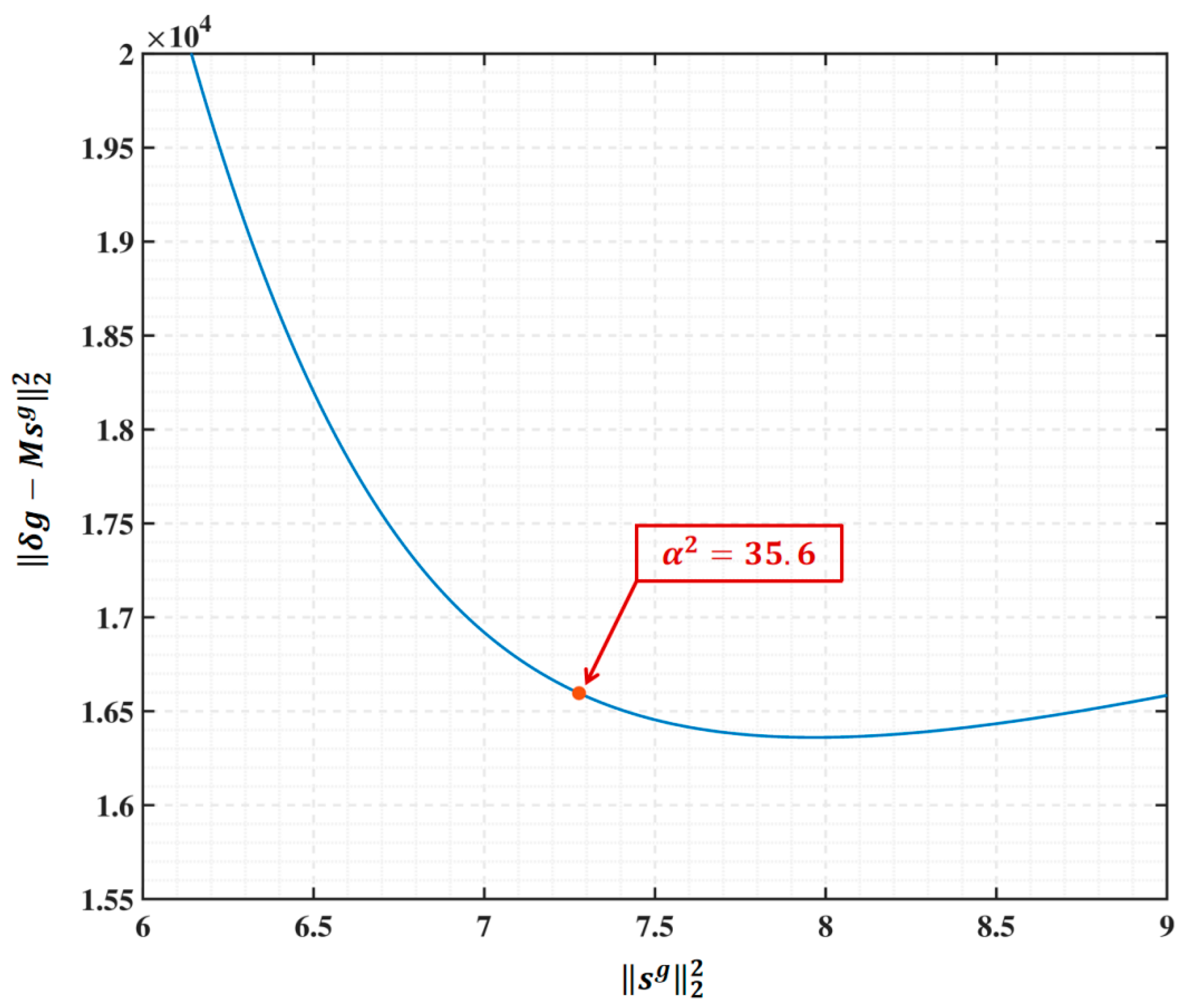
where W is the weighted matrix of gravity disturbances δ g determined by their precision of observation; s g is the Slepian basis coefficient vector for the gravity disturbances. M is the corresponding design matrix for the gravity disturbances and the Slepian function coefficient vector; α 2 is the regularization factor that could weigh and adjust the relative weight between the data fit and roughness, and the optimal solution of α 2 was selected by the L-Curve method as shown in Figure 3 [31].
However, due to significant topographic relief and inaccurate regional long-wave effects, the regional gravity disturbance field derived directly from Equation (10) exhibits certain uncertainties. Therefore, we construct a regional gravity disturbance field in North China following the technical route shown in Figure 4. This approach mitigates the effects of topographic relief and inaccurate long-wave using the remove-compute-restore method [32,33,34]. Simultaneously, the Gibbs phenomenon in Slepian basis expansion is effectively suppressed, as described in Equation (9), by transforming coefficients, adding a window function, and imposing the regional eigenvalue constraint.

3. Datasets

3.1. Global Gravity Field Model

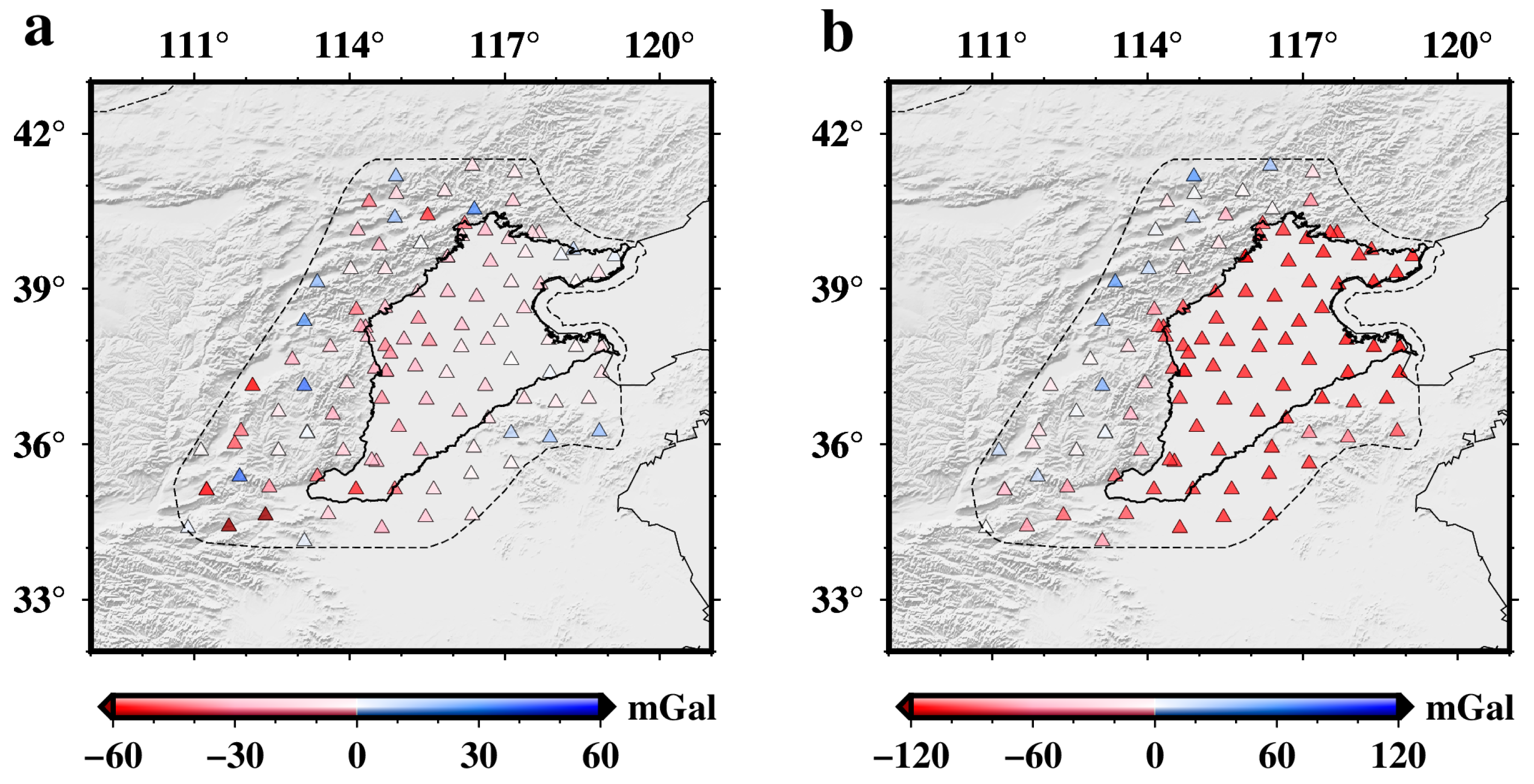
In this study, the EIGEN-6C4 gravity field model released by the German Research Centre for Geosciences (GFZ) was adopted as the global gravity field model, with its spherical harmonic coefficients up to d/o 2190. To calculate the gravity disturbance, we used the Shuttle Radar Topography Mission (SRTM) 30 m resolution DEM data (https://earthexplorer.usgs.gov/, accessed on 20 November 2013) that sampled it at each 0.25° grid. Figure 5a shows the gravity disturbances calculated using the EIGEN-6C4 gravity field model and elevations at each terrestrial gravity station.

3.2. Spherical Harmonic Model of Topographic Gravity Field Model

The dV_SPH_EARTH2014 model has been forward modeled by spectral integration of volumetric mass layers as represented by the Earth2014 topographic database [35]. As in the EIGEN-6C4 gravity field model, the dV_SPH_EARTH2014 model indicates the spherical approximation gravitational potential of topographic relief, with its spherical harmonic coefficients up to d/o 2190 [36]. Thereby, we adopted the dV_SPH_EARTH2014 model (https://ddfe.curtin.edu.au/models/Earth2014/, accessed on 24 August 2016) to calculate the topographic effects (Figure 5b) using a similar formula to Equation (2) at each terrestrial gravity station.

3.3. Terrestrial Gravity Data

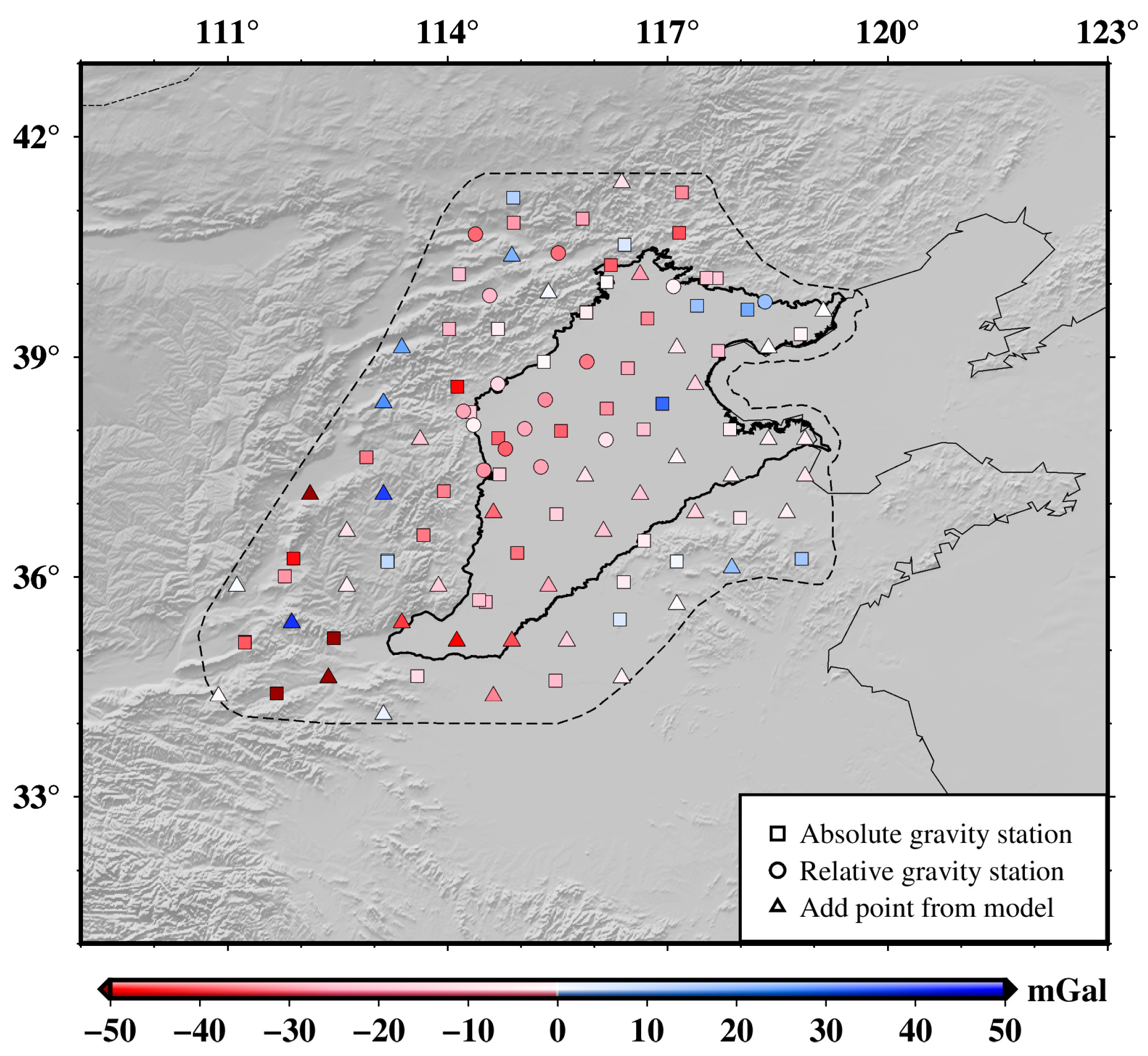
In North China, relying on the National Precision Gravity Measurement Facility (PGMF) project, a total of 55 absolute gravity measurements and 15 relative gravity measurements were collected. The distribution of observation sites is illustrated in Figure 6, with 14 absolute gravity measurements co-located with GNSS observations. The elevations of these 14 gravity observation sites were observed using GNSS stations, while real-time kinematic (RTK) measurements were used for the remaining sites. Due to the interval distance between adjacent stations in some areas of North China being greater than 110 km, an additional 40 sites of gravity disturbance were calculated using the EGM2008 model.

4. Results

4.1. Gibbs Phenomenon

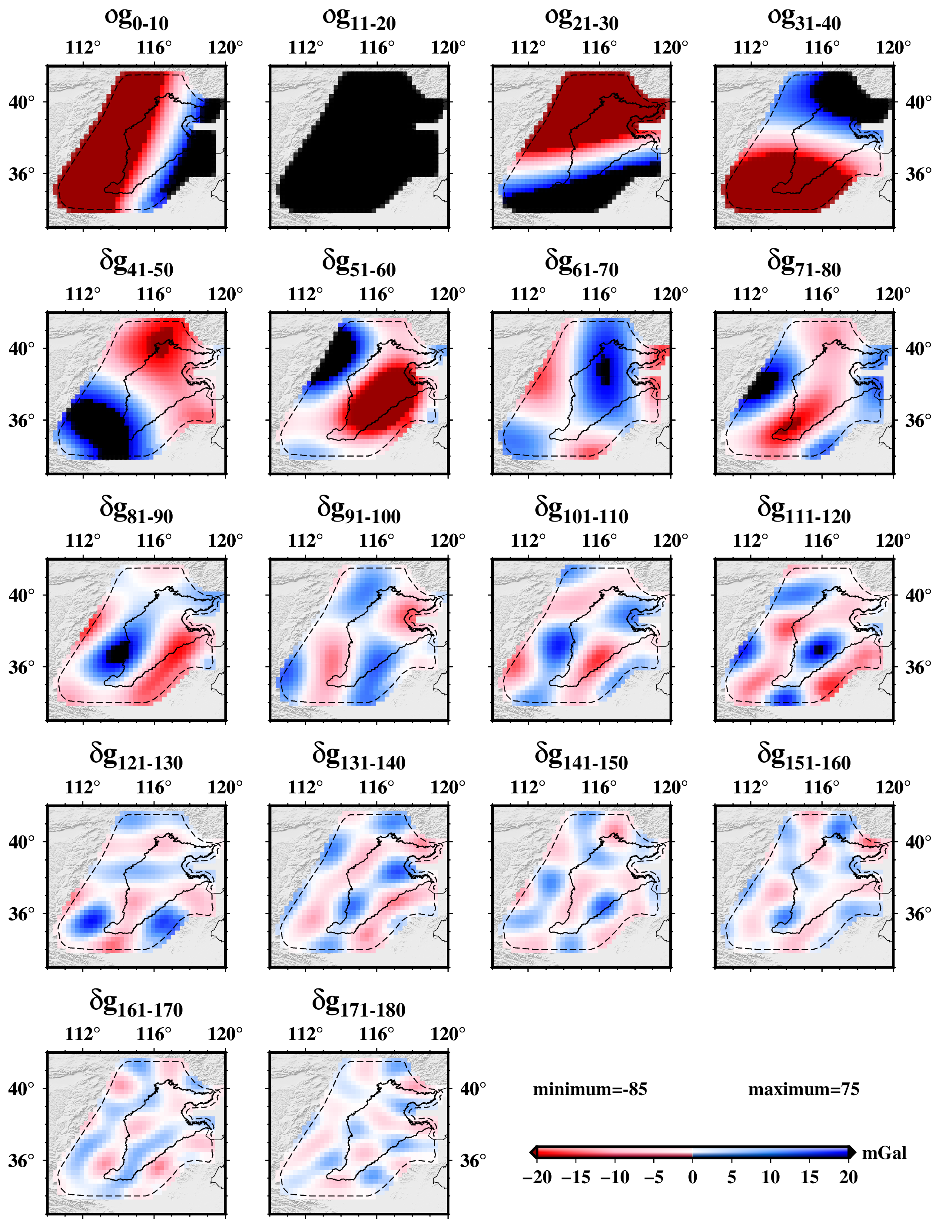
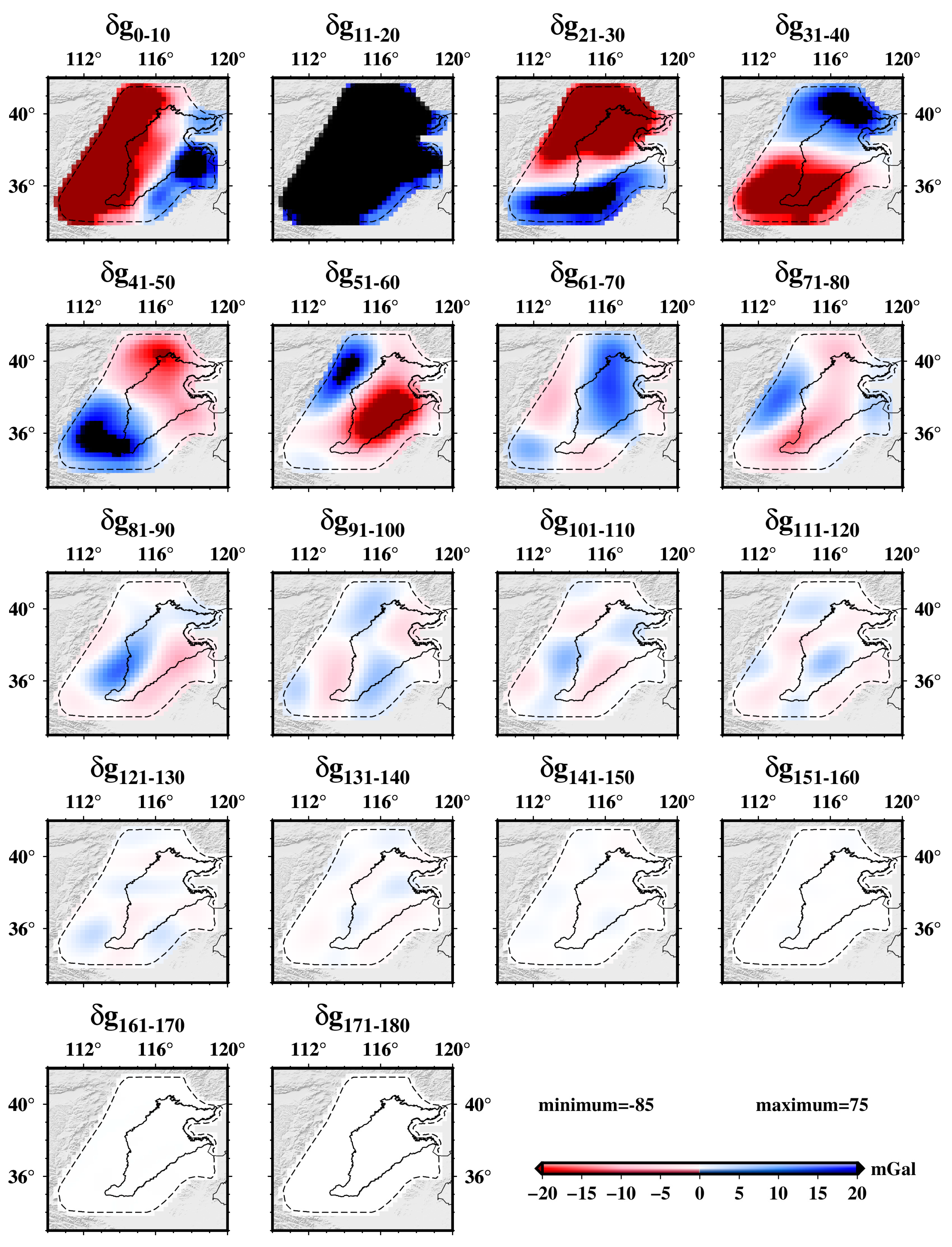
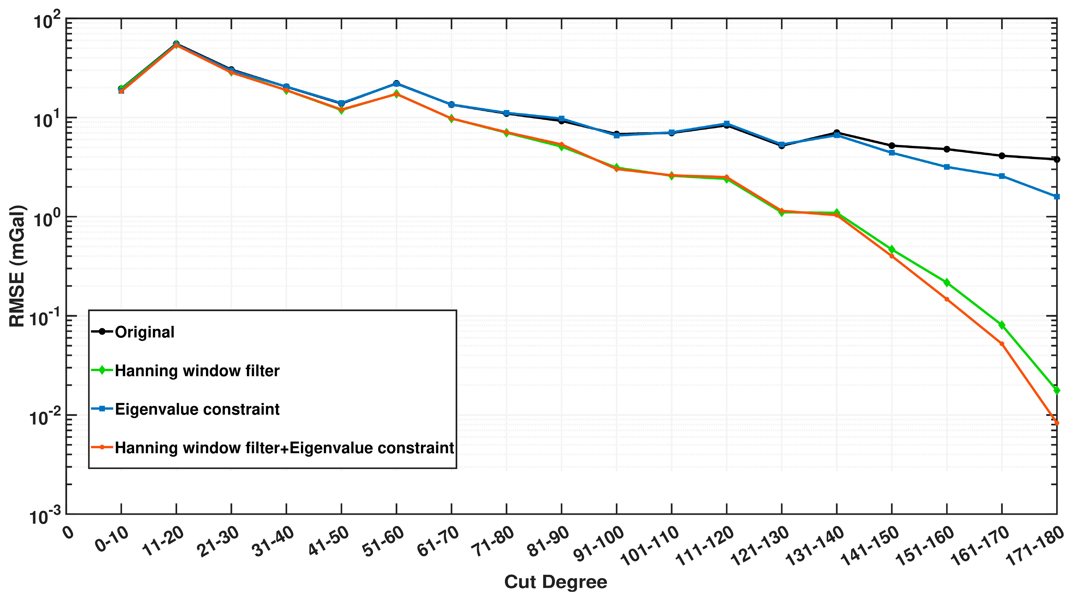
To better observe the Gibbs phenomenon in the spherical harmonic expansion of the EIGEN-6C4 gravity field model, the global 0.25° gridded gravity disturbances, with topographic effects removed, were set to zero in North China and expanded to spherical harmonic functions up to a resolution of 110 km (d/o, 180). The analysis was segmented at every ten d/o of the truncated expansion (e.g., 0–10, 11–20, 21–30 …… 171–180), as illustrated in Figure 7, Figure 8 and Figure 9. Notably, beyond the 90th d/o, the Gibbs phenomenon dominated, exhibiting an RMSE of approximately 10 mGal, while the 0~30th d/o primarily reflected long-wave leakage from outside the North China region (Figure 7 and Figure 9). Following window function filtering and regional eigenvalue constraint processing, depicted in Figure 8 and Figure 9, the Gibbs phenomenon was significantly mitigated beyond the 60th d/o, particularly beyond the 120th d/o, of which the root mean squared errors (RMSE) have been reduced to less than 1 mGal and over 90% of the Gibbs phenomenon has been suppressed. Additionally, comparisons between using window function filtering alone, regional eigenvalue constraint alone, and their combination demonstrated that regional eigenvalue constraint could further diminish high-degree Gibbs phenomena.

4.2. TM-RGD in North China with Gibbs Phenomenon Suppression

The combination of window function filtering and regional eigenvalue constraints enhances the suppression of the high-degree Gibbs phenomenon. Furthermore, due to the ability of the regional eigenvalue constraint to attenuate signal leakage from outside the region, this combination approach more accurately reflects the spatial characteristics of the regional gravity disturbance field compared to using window function filtering alone. We further compared the regional gravity disturbance fields with a spatial resolution of 110 km in North China derived from the EIGEN-6C4 model and the elevation data (Figure 10). As shown in Figure 10a, the field derived by direct spherical harmonic expansion exhibits reductions in gravity disturbances within the North China Plain (NCP) and increases in the western and northern parts of the region. Due to the relatively flat topography of the NCP, the significant negative gravity disturbances of about −40 mGal within this region may primarily be attributed to the Gibbs phenomenon. Although the Gibbs phenomenon in the regional gravity disturbance field in North China has been sensibly suppressed with Hanning window function filtering applied alone (Figure 10b), external leakages have been introduced, particularly at the edges of the region, such as the southern part of North China. In contrast, as shown in Figure 10c, the field derived by the combination approach effectively suppresses the Gibbs phenomenon and reduces external signal leakage. Moreover, the field in Figure 10c distinctly delineates the spatial characteristics of relatively large negative gravity disturbances in the southern and central parts of the North China region. Therefore, the field derived from the EIGEN-6C4 model by the combination approach is more accurate and can be approximated as the ‘true model regional gravity disturbance field’ (TM-RGDF).

4.3. Validation of the TM-RGDF with TGD-RGDF

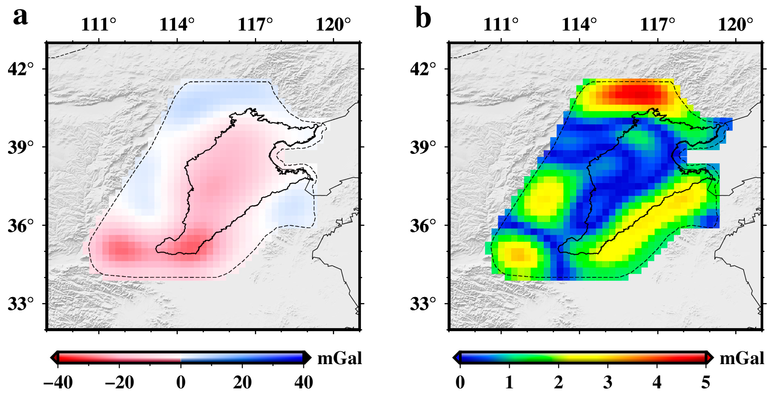
Based on the approach outlined in Figure 4, we constructed the TGD-RGDF based on Slepian basis functions and terrestrial gravity data. In the long-wave effects remove-compute-restore process, we selected the 0–30th d/o long-wave components and derived the TGD-RGDF from the terrestrial data with a resolution of 110 km. As shown in Figure 11a, this TGD-RGDF is highly consistent in spatial distribution with the TM-RGDF from the EIGEN-6C4 model (Figure 10c), with an overall RMSE of 0.80 mGal and a correlation coefficient of 0.99 in the spatial domain. Better agreement between TM-RGDF and TGD-RGDF further confirms the effectiveness of the combination approach, compared to the original and Hanning window function filtering results (Figure 10a,b) from the EIGEN-6C4 model.
The largest error of TM-RGDF is located in the northern part of North China (Figure 11b), where the distribution of terrestrial gravity stations is relatively sparse (Figure 6). Thus, the insufficient distribution of stations may be one of the main factors contributing to the error in constructing the TGD-RGDF from terrestrial data. Additionally, errors in gravity observations and elevations also impact the accuracy of the constructed TGD-RGDF.

5. Discussions

5.1. Effects on Removing and Restoring Global Medium-Long Wave Signals in Different Degrees

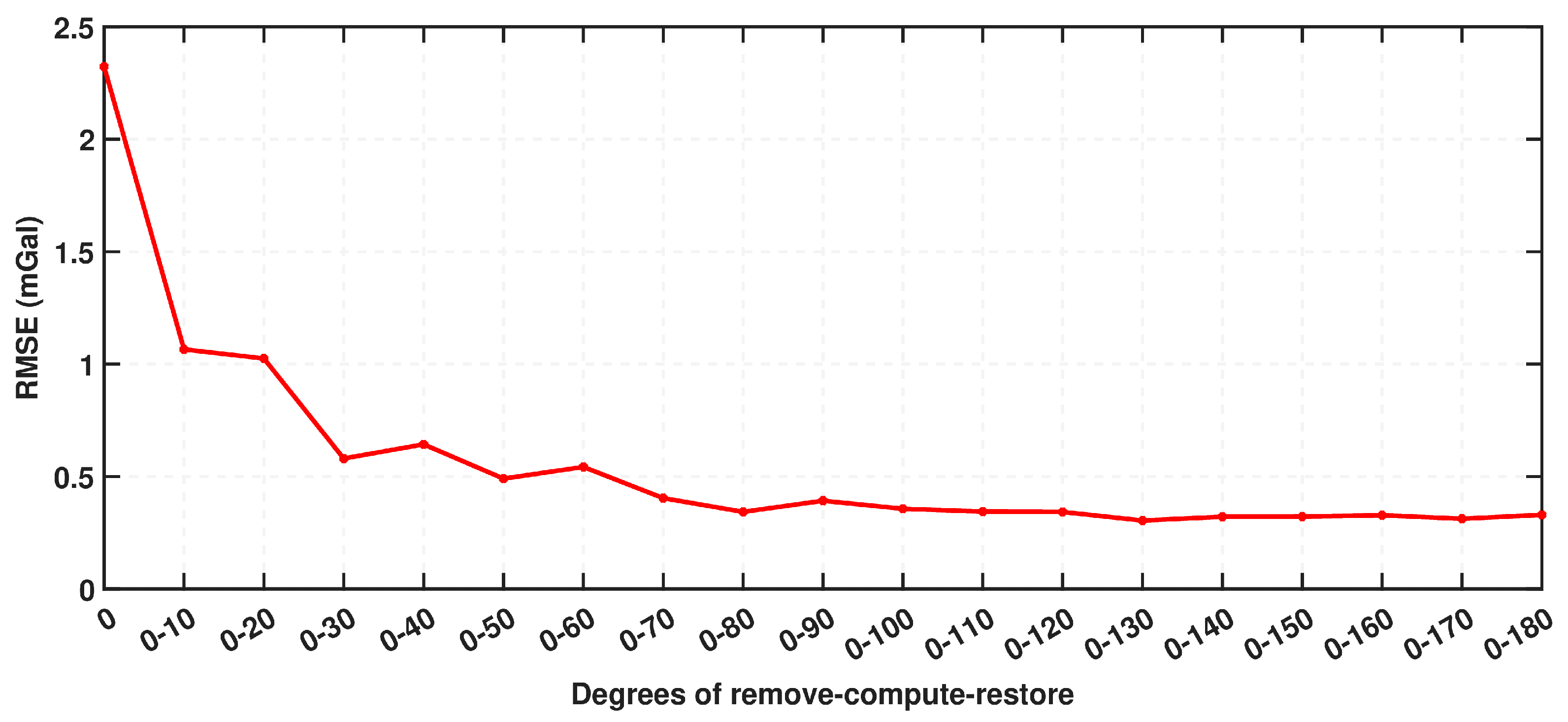
When constructing a TGD-RGDF from terrestrial gravity data, inaccuracies in the long-wave signal of the regional gravity field are inevitable due to insufficient regional coverage. In this study, using the North China region as an example, which spans approximately 6° by 6°, not employing the global long-wave remove-compute-restore method results in an error of about 2.4 mGal, as demonstrated in Figure 12. This figure also indicates that effective results can be achieved by removing and restoring global long waves from the 0–30th d/o. The spatial resolution of 660 km, corresponding to the 0–30th d/o, matches the regional extent. Furthermore, removing and restoring global medium-long wave signals does not necessarily lead to errors decreasing when higher d/o are removed. For instance, removing and restoring the 0–40th d/o leads to increased errors compared to the removal and restoral of the 0–30th d/o, possibly due to irregularities in the shape of the region boundary.

5.2. The Impact of Insufficient Stations’ Distribution on Constructing Regional Gravity Disturbance Field

When constructing a TGD-RGDF from terrestrial gravity data, the discrepancy between the gravity disturbance and the model’s true value is predominantly observed in areas with sparse station distribution. Consequently, we further constructed a regional gravity disturbance field solely from terrestrial gravity observational data (Figure 13a) without employing the EGM2008 model to calculate additional gravity disturbance points, i.e., only the stations with square and circle symbols used in Figure 6. Based on this field, the RMSE of the gravity disturbance in the North China Plain is approximately 3.3 mGal (Figure 13b), more than three times higher than that from TGD-RGDF (Figure 11b). The largest errors are mainly found in areas with the lowest station density, such as the southeast side of the North China Plain. These errors are primarily attributed to over-fitting by the regional Slepian basis functions corresponding to the 0–180th d/o spherical harmonic functions in areas where the station distribution density is less than one per 110 km. However, not all areas with sparse station distribution necessarily exhibit a significant increase in the gravity disturbance field error, such as the western areas outside the North China Plain. The reason may be that, although these regions have insufficient station coverage, the stations are optimally positioned at the principal feature points of the basis function fitting, thereby avoiding over-fitting issues.

5.3. Differences of the Filtered Results by Using Various Window Functions

Except for the Hanning window functions, other commonly utilized window functions, such as the Lanczos and Gaussian windows, can also effectively suppress the Gibbs phenomenon. The expressions for the Lanczos and Gaussian window functions in the spherical harmonic domain are as follows:
W 0 L = 1 , W n L = sin π n / N + 1 / π n / N + 1 , 1 n N ,
b = ln 2 / 1 cos r / a , W 0 G = 1 ,   W 1 G = 1 + e 2 b 1 e 2 b 1 b , W n + 1 G = 2 n + 1 b W n G + W n 1 G , 1 n 60 , W n G = e x p n r / a 2 4 ln 2 , 61 n N ,
where W n L and W n G indicate the Lanczos and Gaussian window functions in the spherical harmonic domain, respectively; r is the averaging radius and set as 110 km; a is the Earth’s mean radius and b is a dimensionless parameter that defines the smoothing process of the Gaussian operator. For Gaussian window functions, as the accurate iterative solution exhibits instabilities when beyond d/o 60, an approximate calculation is employed [37,38].
The Lanczos and Gaussian window functions are employed to filter the EIGEN-6C4 model to suppress the Gibbs phenomenon, similar to Equation (3). The results obtained from these window filters demonstrate high spatial consistency with those derived using the Hanning window filter (Figure 10b and Figure 14a,b), exhibiting a correlation coefficient of 0.99 in the spatial domain. Indeed, due to the differences in mainlobe widths and sidelobe heights of various window filters, the filtering results obtained using different windows exhibit some variability. Figure 14c,d illustrate the differences in the results obtained using Lanczos and Gaussian windows compared to those using the Hanning window, with root mean square values of 1.32 mGal and 0.82 mGal, respectively. Nevertheless, this does not affect the validation results between TM-RGDF and TGD-RGDF. When the Hanning window is replaced with Lanczos or Gaussian windows, the RMSEs between TM-RGDF and TGD-RGDF are 0.85 mGal and 0.83 mGal, respectively, consistent with the result of 0.80 mGal from the Hanning window.

5.4. Differences of TM-RGDFs from Various GGMs in North China

In addition to the EIGEN-6C4 model, other ultra-high-degree GGMS (e.g., EGM2008, XGM2019e, and SGG-UGM-2) can also be utilized to derive the TM-RGDF in North China with a spatial resolution of 110 km. Consequently, by comparing TM-RGDFs derived from various GGMs with TGD-RGDF, the accuracy of each GGM can be assessed. Comparisons indicate that TM-RGDFs obtained from the EGM2008, XGM2019e, and SGG-UGM-2 models also exhibit high spatial consistency with the TGD-RGDF in North China (Figure 15), all with an RMSE of approximately 0.80 mGal and a spatial correlation coefficient of 0.99. This consistency underscores the comparable accuracy of these models at a spatial resolution of 110 km in North China.

6. Conclusions

The combination of window function filtering and regional eigenvalue constraint methods effectively mitigates the Gibbs phenomenon associated with spherical harmonic functions during the regional expansion of the gravity field model. When the EIGEN-6C4 model employing spherical harmonic expansion is truncated to the d/o 180 (110 km spatial resolution) in North China, this combination approach effectively suppresses the Gibbs phenomenon, particularly for the d/o beyond 120th, reducing over 90% of its effects. This approach can also significantly decrease signal leakage outside the region and restore the spatial distribution characteristics within the North China region.
Compared with the TM-RGDF obtained from the EIGEN-6C4 model by the combination approach in North China, the TGD-RGDF constructed using terrestrial gravity data exhibits consistent spatial distribution, with an overall RMSE of 0.80 mGal. This comparison further validates the combination method’s effectiveness in mitigating the Gibbs phenomenon and reducing signal leakage outside the research area. Consequently, this approach can be utilized to accurately derive regional gravity fields, thereby facilitating the establishment of unified regional elevation benchmarks and enabling the inversion of the Earth’s internal structure at a regional scale. Furthermore, the approach proposed in this study holds the potential to improve the accuracy of regional mass changes inferred from GNSS displacements or gravity changes.

Author Contributions

Conceptualization, Y.S. and W.F.; methodology, Y.S.; software, Y.S.; validation, Y.S., W.F., M.Z. and M.Y.; formal analysis, Y.S. and M.Y.; investigation, Y.S., W.T. and Y.X.; resources, Y.S., W.T. and Y.X.; data curation, Y.S. and W.T.; writing—original draft preparation, Y.S.; writing—review and editing, W.F., M.Z., M.Y. and Z.J.; visualization, Y.S.; supervision, W.F. and M.Z.; project administration, Y.S.; funding acquisition, W.F., M.Z., M.Y. and Y.S. All authors have read and agreed to the published version of the manuscript.

Funding

This research was funded by the Fundamental National Natural Science Foundation of China (42027802, 42104083) and the Open Research Fund Program of the State Key Laboratory of Geodesy and Earth’s Dynamics (SKLGED2022-2-4). This research was also funded by the National Precise Gravity Measurement Facility, Huazhong University of Science and Technology, Wuhan 430074, China.

Data Availability Statement

The GGMs such as EIGEN-6C4, EGM2008, XGM2019e and SGG-UGM-2 models in this research can be available from the website http://icgem.gfz-potsdam.de/home, accessed on 28 November 2014, 19 April 2012, 17 October 2019 and 8 June 2020, respectively. The SRTM DEM data can be available from https://earthexplorer.usgs.gov/, accessed on 20 November 2013. The dV_SPH_EARTH2014 model can be available from https://ddfe.curtin.edu.au/models/Earth2014/, accessed on 24 August 2016.The terrestrial gravity measurements are confidential, and it is illegal to provide these measurements directly, according to Chinese regulations. The processed terrestrial gravity disturbances with their elevations can be available upon request.

Acknowledgments

The regional Slepian basis functions are calculated using the SLEPIAN suite hosted by the Community Surface Dynamics Modeling System Group at the University of Colorado, Boulder (https://csdms.colorado.edu/wiki/Model:SLEPIAN_Alpha, accessed on 1 November 2014). The gravity disturbance is based on the gravity field model computed by the Graflab program, usage of the Graflab program is subject to licensing (https://github.com/blazej-bucha/isgraflab, accessed on 1 November 2019). We also appreciate the anonymous reviewers whose insights helped to improve this manuscript.

Conflicts of Interest

The authors declare no conflict of interest.

References

  1. Pavlis, N.K.; Holmes, S.A.; Kenyon, S.C.; Factor, J.K. The development and evaluation of the Earth Gravitational Model 2008 (EGM2008): THE EGM2008 EARTH GRAVITATIONAL MODEL. J. Geophys. Res. Solid Earth 2012, 117, B04406. [Google Scholar] [CrossRef]
  2. Bruinsma, S.; Abrykosov, O.; Lemoine, J.M. The latest combined global gravity field model including GOCE data up to degree and order 2190 of GFZ Potsdam and GRGS Toulouse (EIGEN 6C4). In Proceedings of the 5th GOCE User Workshop, Paris, France, 25–28 November 2014; pp. 25–28. [Google Scholar]
  3. Liang, W.; Li, J.; Xu, X.; Zhang, S.; Zhao, Y. A high-resolution Earth’s gravity field model SGG-UGM-2 from GOCE, GRACE, satellite altimetry, and EGM2008. Engineering 2020, 6, 860–878. [Google Scholar] [CrossRef]
  4. Zingerle, P.; Pail, R.; Gruber, T.; Oikonomidou, X. The combined global gravity field model XGM2019e. J. Geod. 2020, 94, 66. [Google Scholar] [CrossRef]
  5. Lemoine, F.G.; Kenyon, S.C.; Factor, J.K.; Trimmer, R.G.; Pavlis, N.K.; Chinn, D.S.; Cox, C.M.; Klosko, S.M.; Luthcke, S.B.; Torrence, M.H. The Development of the Joint NASA GSFC and the National Imagery and Mapping Agency (NIMA) Geopotential Model EGM96; NASA: Washington, DC, USA, 1998. [Google Scholar]
  6. Reigber, C.; Schwintzer, P.; Stubenvoll, R.; Schmidt, R.; Flechtner, F.; Meyer, U.; König, R.; Neumayer, K.-H.; Förste, C.; Barthelmes, F. A High Resolution Global Gravity Field Model Combining CHAMP and GRACE Satellite Mission and Surface Data: EIGEN-CG01C; Deutsches Geo Forschungs Zentrum GFZ: Potsdam, Germany, 2006. [Google Scholar]
  7. Bomfim, E.; Braitenberg, C.; Molina, E.C. Mutual evaluation of global gravity models (EGM2008 and GOCE) and terrestrial data in Amazon Basin, Brazil. Geophys. J. Int. 2013, 195, 870–882. [Google Scholar] [CrossRef]
  8. Yahaya, S.I.; El Azzab, D. Assessment of recent GOCE-based global geopotential models and EGM2008 in Niger Republic. Geod. Cartogr. 2019, 45, 116–125. [Google Scholar] [CrossRef]
  9. Hirt, C.; Marti, U.; Bürki, B.; Featherstone, W.E. Assessment of EGM2008 in Europe using accurate astrogeodetic vertical deflections and omission error estimates from SRTM/DTM2006. 0 residual terrain model data. J. Geophys. Res. Solid Earth 2010, 115, B10404. [Google Scholar] [CrossRef]
  10. Godah, W.; Krynski, J.; Szelachowska, M. The use of absolute gravity data for the validation of Global Geopotential Models and for improving quasigeoid heights determined from satellite-only Global Geopotential Models. J. Appl. Geophys. 2018, 152, 38–47. [Google Scholar] [CrossRef]
  11. Novák, P.; Kostelecký, J.; Klokočník, J. Testing global geopotential models through comparison of a local quasi-geoid model with GPS/leveling data. Stud. Geophys. Geod. 2009, 53, 39–60. [Google Scholar] [CrossRef]
  12. Odumosu, J.O.; Nnam, V.C.; Nwadialor, I.J. An assessment of spatial methods for merging terrestrial with GGM-derived gravity anomaly data. J. Afr. Earth Sci. 2021, 179, 104202. [Google Scholar] [CrossRef]
  13. Varga, M.; Pitoňák, M.; Novák, P.; Bašić, T. Contribution of GRAV-D airborne gravity to improvement of regional gravimetric geoid modelling in Colorado, USA. J. Geod. 2021, 95, 53. [Google Scholar] [CrossRef]
  14. Nyoka, C.J.; Din, A.H.M.; Pa’suya, M.F.; Omar, A.H. Rigorous evaluation of global geopotential models for geoid modelling: A case study in Kenya. J. Afr. Earth Sci. 2022, 194, 104612. [Google Scholar] [CrossRef]
  15. Voigt, C.; Denker, H. Validation of GOCE gravity field models in Germany. Newton’s Bull. 2015, 5, 37–49. [Google Scholar]
  16. Zhao, D.J.; Zhang, M.L.; Wang, Q.; Cheng, Y.X. Accuacy analyses of EIGEN-6C2 Geopotential model in China mainland. J. Geod. Geodyn. 2014, 34, 21–24. [Google Scholar]
  17. Hirt, C.; Gruber, T.; Featherstone, W. Evaluation of the first GOCE static gravity field models using terrestrial gravity, vertical deflections and EGM2008 quasigeoid heights. J. Geod. 2011, 85, 723–740. [Google Scholar] [CrossRef]
  18. Sjüberg, L. Quality estimates in geoid computation by EGM08. J. Geod. Sci. 2011, 1, 361–366. [Google Scholar] [CrossRef]
  19. Albertella, A.; Sansò, F.; Sneeuw, N. Band-limited functions on a bounded spherical domain: The Slepian problem on the sphere. J. Geod. 1999, 73, 436–447. [Google Scholar] [CrossRef]
  20. Simons, F.J.; Dahlen, F.; Wieczorek, M.A. Spatiospectral concentration on a sphere. SIAM Rev. 2006, 48, 504–536. [Google Scholar] [CrossRef]
  21. Slepian, D. Prolate spheroidal wave functions, Fourier analysis and uncertainty—IV: Extensions to many dimensions; generalized prolate spheroidal functions. Bell Syst. Tech. J. 1964, 43, 3009–3057. [Google Scholar] [CrossRef]
  22. Jiang, Z.; Hsu, Y.-J.; Yuan, L.; Cheng, S.; Li, Q.; Li, M. Estimation of daily hydrological mass changes using continuous GNSS measurements in mainland China. J. Hydrol. 2021, 598, 126349. [Google Scholar] [CrossRef]
  23. Han, S.C.; Mahdiyeh Razeghi, S. GPS recovery of daily hydrologic and atmospheric mass variation: A methodology and results from the Australian continent. J. Geophys. Res. Solid Earth 2017, 122, 9328–9343. [Google Scholar] [CrossRef]
  24. Han, J.C.; Chen, S.; Lu, H.Y.; Jia, L.L.; Wang, L.H.; Xu, W.M.; Zhang, H.; Sun, H.P. A high-resolution time-variable terrestrial gravity field model of continental North China. Commun. Earth Environ. 2024, 5, 44. [Google Scholar] [CrossRef]
  25. Shim, H.-T.; Volkmer, H.; Walter, G.G. Gibbs’ phenomenon in higher dimensions. J. Approx. Theory 2007, 145, 20–32. [Google Scholar] [CrossRef]
  26. Jerri, A.J. The Gibbs Phenomenon in Fourier Analysis, Splines and Wavelet Approximations; Springer Science & Business Media: Berlin/Heidelberg, Germany, 1998; Volume 446. [Google Scholar]
  27. Sloan, P.-P. Stupid spherical harmonics (sh) tricks. In Proceedings of the Game Developers Conference, San Francisco, CA, USA, 18–22 February 2008; p. 42. [Google Scholar]
  28. Klees, R.; Tenzer, R.; Prutkin, I.; Wittwer, T. A data-driven approach to local gravity field modelling using spherical radial basis functions. J. Geod. 2008, 82, 457–471. [Google Scholar] [CrossRef]
  29. Hwang, C.; Hsu, H.-J.; Chang, E.T.; Featherstone, W.; Tenzer, R.; Lien, T.; Hsiao, Y.-S.; Shih, H.-C.; Jai, P.-H. New free-air and Bouguer gravity fields of Taiwan from multiple platforms and sensors. Tectonophysics 2014, 611, 83–93. [Google Scholar] [CrossRef]
  30. Han, J.C.; Chen, S.; Lu, H.Y.; Xu, W.M. Time-variable gravity field determination using Slepian functions and terrestrial measurements: A case study in North China with data from 2011 to 2013. Chin. J. Geophys. 2021, 64, 1542–1557. [Google Scholar]
  31. O’Leary, D.P.; Hansen, P.C. The use of the L-Curve in the regularization of discrete ill-posed problems. SIAM J. Sci. Comput. 1993, 14, 1487–1503. [Google Scholar]
  32. Kalu, I.; Ndehedehe, C.E.; Okwuashi, O.; Eyoh, A.E. Integration of satellite geodetic observations for regional geoid modeling using remove-compute-restore technique. Earth Sci. Inform. 2022, 15, 233–251. [Google Scholar] [CrossRef]
  33. Sjöberg, L.E. Unbiased least-squares modification of Stokes’ formula. J. Geod. 2020, 94, 92–94. [Google Scholar] [CrossRef]
  34. Yildiz, H.; Forsberg, R.; Ågren, J.; Tscherning, C.; Sjöberg, L. Comparison of remove-compute-restore and least squares modification of Stokes’ formula techniques to quasi-geoid determination over the Auvergne test area. J. Geod. Sci. 2012, 2, 53–64. [Google Scholar] [CrossRef]
  35. Hirt, C.; Rexer, M. Earth2014: 1 arc-min shape, topography, bedrock and ice-sheet models–Available as gridded data and degree-10,800 spherical harmonics. Int. J. Appl. Earth Obs. Geoinf. 2015, 39, 103–112. [Google Scholar] [CrossRef]
  36. Rexer, M.; Hirt, C.; Claessens, S.; Tenzer, R. Layer-based modelling of the Earth’s gravitational potential up to 10-km scale in spherical harmonics in spherical and ellipsoidal approximation. Surv. Geophys. 2016, 37, 1035–1074. [Google Scholar] [CrossRef]
  37. Wahr, J.; Molenaar, M.; Bryan, F. Time variability of the Earth’s gravity field: Hydrological and oceanic effects and their possible detection using GRACE. J. Geophys. Res. Solid Earth 1998, 103, 30205–30229. [Google Scholar] [CrossRef]
  38. Chambers, D.P. Observing seasonal steric sea level variations with GRACE and satellite altimetry. J. Geophys. Res. Ocean. 2006, 111, C03010. [Google Scholar] [CrossRef]
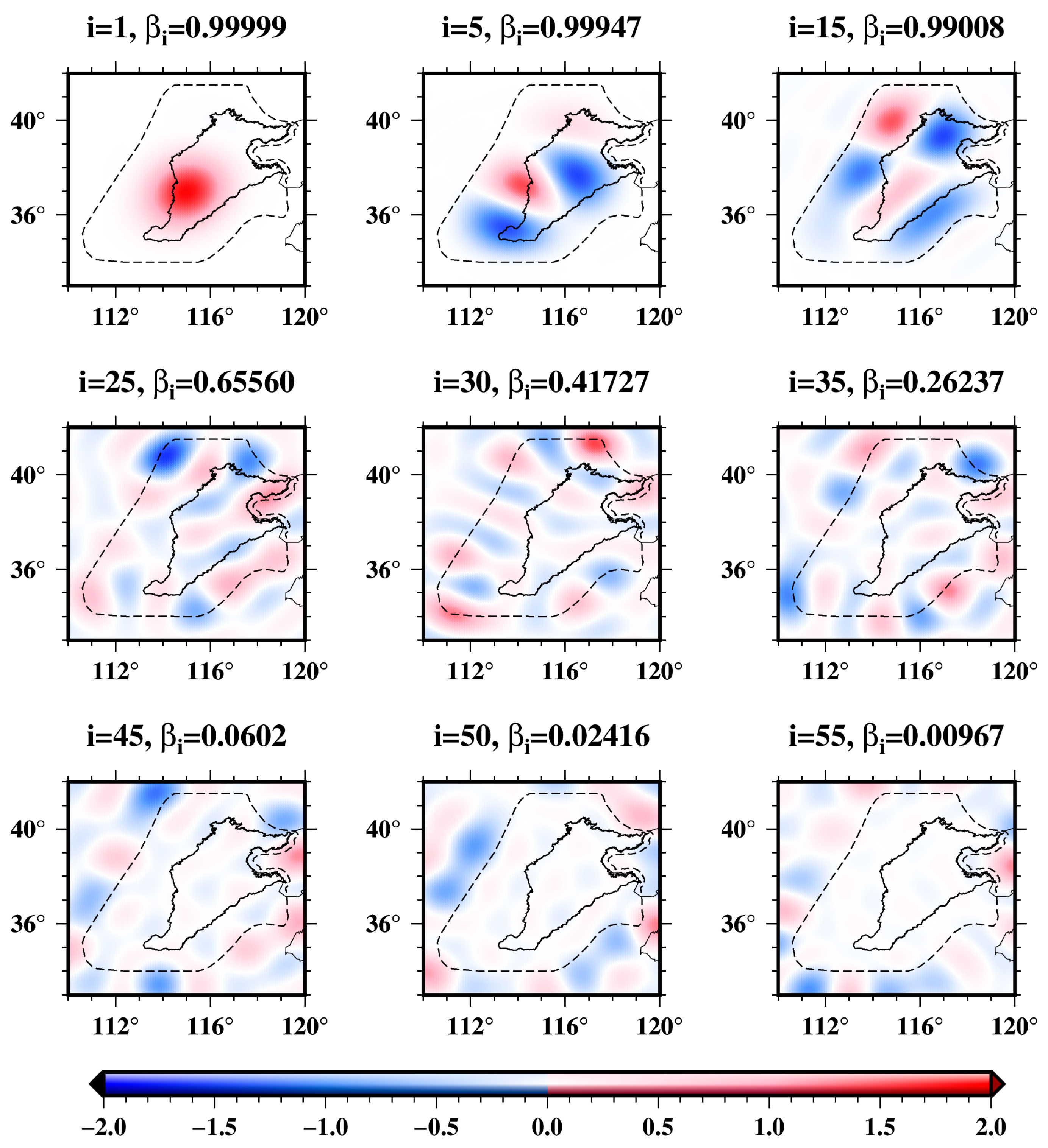
Figure 1. Examples of the Slepian basis functions f i θ , λ in North China. The boundary shown in the black dashed line is used to compute the regional basis functions. The black solid line represents the boundary of the North China Plain (NCP). The eigenvalue β i indicates the energy concentration ratio.
Remotesensing 16 02756 g001
Figure 2. Concentration ratio β i for each Slepian basis function. The total number of Slepian basis functions is 32,761 with a maximum degree of N = 180; The first Ncut = 55 functions have concentration ratios above 0.01 and are used to recover the water storage changes in North China.
Remotesensing 16 02756 g002
Figure 3. L-Curve to determine the optimal regularization factor for the object function Equation (10). The optimal regularization factor is determined as α 2 = 35.6 , by calculating the corresponding α 2 at the point of maximum curvature based on the curvature formula from O’Leary and Hansen (1993) [31].
Remotesensing 16 02756 g003
Figure 4. Technological route map of constructing regional gravity disturbance field based on ground gravity disturbances. The terms ‘remove-compute-restore 1’ and ‘remove-compute-restore 2’ refer to the processes of removing and restoring topographic effects and global long-wave effects, respectively.
Remotesensing 16 02756 g004
Figure 5. Gravity disturbance and topographic effects at each terrestrial gravity station. (a), the gravity disturbance based on the EIGEN-6C4 gravity field model and elevations; (b), topographic effects based on the dV_SPH_EARTH2014 topographic gravity field model and elevations. The triangles represent the terrestrial gravity stations. The boundary shown by the black dashed line indicates the coverage of the gravity stations. The black solid line denotes the boundary of the NCP.
Remotesensing 16 02756 g005
Figure 6. Distribution of gravity disturbances in the North China region. The square, circle, and triangle represent the absolute gravity station, relative gravity station, and additional EGM2008 model site, respectively. The color bar scale represents the value of the gravity disturbance.
Remotesensing 16 02756 g006
Figure 7. Gibbs phenomenon in the North China Region, induced by the spherical harmonic expansion of gravity disturbances (with topographic effects removed), is obtained from EIGEN-6C4 and dV_SPH_EARTH2014 models at the global 0.25° grid. The black dashed line marks the boundary of the region within which the global 0.25° grid gravity disturbances from EIGEN-6C4 and dV_SPH_EARTH2014 models have been set to zero. The global 0.25° grid gravity disturbances (with topographic effects removed) are expanded into spherical harmonic functions up to a resolution of 110 km (d/o 180). Every ten d/o of the spherical harmonic functions were segmented for more detailed observation and analysis (e.g., 0–10th, 11–20th, 21–30th, … 171–180th).
Remotesensing 16 02756 g007
Figure 8. The suppressed Gibbs phenomenon results for Figure 7, using the combination of window function and regional eigenvalue constraint method. The black dashed line marks the boundary of the region within which the global 0.25° grid gravity disturbances from EIGEN-6C4 and dV_SPH_EARTH2014 models have been set to zero. The global 0.25° grid gravity disturbances (with topographic effects removed) are expanded into spherical harmonic functions up to a resolution of 110 km (d/o 180). Every ten d/o of the spherical harmonic functions were segmented for more detailed observation and analysis (e.g., 0–10th, 11–20th, 21–30th, … 171–180th).
Remotesensing 16 02756 g008
Figure 9. Comparison of the suppressed Gibbs phenomenon results of using window function filtering alone, regional eigenvalue constraint alone, and their combination approach to the original results in Figure 7. The black line represents the original results for the Gibbs phenomenon. The green line shows the suppressed Gibbs phenomenon results using Hanning window filtering alone. The blue line displays the suppressed Gibbs phenomenon results using regional eigenvalue constraint alone. The red line indicates the suppressed Gibbs phenomenon results using the combination approach.
Remotesensing 16 02756 g009
Figure 10. Regional gravity disturbance field based on EIGEN-6C4 model and its suppressed Gibbs phenomenon results. (a), regional gravity disturbance field obtained directly from the EIGEN-6C4 model; (b), same as (a) but the Hanning window filtering applied; (c), same as (a) but the combination of window function and regional eigenvalue constraint method applied. The boundary shown by the black dashed line indicates the coverage of the gravity stations in Figure 6.
Remotesensing 16 02756 g010
Figure 11. TGD-RGDF is derived from terrestrial gravity data and its RMSE distribution in North China. (a), TGD-RGDF constructed from terrestrial gravity data by the approach in Figure 4, gridding by Slepian basis function interpolation method at 0.25°; (b), the distribution of RMSE in North China, calculated by the TGD-RGDF and the TM-RGDF.
Remotesensing 16 02756 g011
Figure 12. Analysis of the RMSE for removing and restoring global medium-long wave signals within different d/o. The RMSE is calculated by the regional gravity disturbance field (constructed by the approach in Figure 4, using the 0.25° grid gravity disturbances from EIGEN-6C4 model within North China) and the TM-RGDF.
Remotesensing 16 02756 g012
Figure 13. TGD-RGDF derived from terrestrial gravity data (without using the EGM2008 model sites) and its RMSE distribution in North China. (a), TGD-RGDF constructed from terrestrial gravity data (without using the EGM2008 model sites in Figure 6) by the approach in Figure 4, gridding by Slepian basis function interpolation method at 0.25°; (b), the distribution of RMSE in North China, calculated by the TGD-RGDF derived from the terrestrial gravity data (without using the EGM2008 model sites in Figure 6) and the TM-RGDF.
Remotesensing 16 02756 g013
Figure 14. Filtered results for the EIGEN-6C4 model using other windows and differences between these results and those filtered by Hanning window. (a), the filtered results for the EIGEN-6C4 model using Lanczos window, with a spatial resolution of 110 km in North China; (b), the same as (a) but the Guassian window applied; (c), the differences between the filtered results using Lanczos window and those filtered by Hanning window; (d), same as (c) but the Guassian window applied.
Remotesensing 16 02756 g014
Figure 15. TM-RGDFs derived from other ultra-high-degree GGMS and their RMSE distribution in North China. (a), TM-RGDF derived from the EGM2008 model with a spatial resolution of 110 km in North China; (b), same as (a) but the XGM2019e model applied; (c), same as (a) but the SGG-UGM-2 model applied; (d), the distribution of RMSE in North China, calculated by the TGD-RGDF and the EGM2008 model-based TM-RGDF; (e), same as (d) but the XGM2019e model-based TM-RGDF applied; (f), same as (d) but the SGG-UGM-2 model-based TM-RGDF applied.
Remotesensing 16 02756 g015
Disclaimer/Publisher’s Note: The statements, opinions and data contained in all publications are solely those of the individual author(s) and contributor(s) and not of MDPI and/or the editor(s). MDPI and/or the editor(s) disclaim responsibility for any injury to people or property resulting from any ideas, methods, instructions or products referred to in the content.