Optimizing Slender Target Detection in Remote Sensing with Adaptive Boundary Perception

Abstract

Over the past few years, target detectors that utilize Convolutional Neural Networks have gained extensive application in the domain of remote sensing (RS) imagery. Recently, optimizing bounding boxes has consistently been a hot topic in the research field. However, existing methods often fail to take into account the interference caused by the shape and orientation changes of RS targets with high aspect ratios during training, leading to challenges in boundary perception when dealing with RS targets that have large aspect ratios. To deal with this challenge, our study introduces the Adaptive Boundary Perception Network (ABP-Net), a novel two-stage approach consisting of pre-training and training phases, which enhances the boundary perception of CNN-based detectors. In the pre-training phase, involving the initialization of our model’s backbone network and the label assignment, the traditional label assignment with a fixed IoU threshold fails to fully cover the critical information of slender targets, resulting in the detector missing lots of high-quality positive samples. To overcome this drawback, we design a Shape-Sensitive (S-S) label assignment strategy that can improve the boundary shape perception by dynamically adjusting the IoU threshold according to the aspect ratios of the targets so that the high-quality samples with critical features can be divided into positive samples. Moreover, during the training phase, minor angle differences of the slender bounding box may cause a significant change in the value of the loss function, producing unstable gradients. Such drastic gradient changes make it difficult for the model to find a stable update direction when optimizing the bounding box parameters, resulting in difficulty with the model convergence. To this end, we propose the Robust–Refined loss function (R-R), which can enhance the boundary localization perception by focusing on low-error samples and suppressing the gradient amplification of difficult samples, thereby improving the model stability and convergence. Experiments on UCAS-AOD and HRSC2016 datasets validate our specialized detector for high-aspect-ratio targets, improving performance, efficiency, and accuracy with straightforward operation and quick deployment.

1. Introduction

Aerial object detection plays an important role in important areas such as environmental monitoring, military reconnaissance, urban planning, and so on. Traditional object detection methods, such as feature extractors based on manual operators and sliding window strategies, are often limited by computational efficiency and accuracy when dealing with large-scale and high-resolution RS data, and have the shortcomings of weak feature expression ability and insufficient robustness.

However, the advent of Convolutional Neural Networks (CNNs) has led to the dominance of deep learning in object detection, with one-stage detectors like SSD [1], RetinaNet [2], and YOLO [3,4,5], which directly process images for object detection without region proposals, becoming popular. Two-stage detectors [6,7,8,9,10], such as Faster R-CNN [8] and Mask R-CNN [10], use a two-stage process involving using region proposal networks to identify potential object regions (ROIs) and subsequent feature extraction for precise bounding box regression and classification. Despite advancements in feature representation, existing methods often fail to fully consider the objective of enhancing the adaptability of the bounding boxes to various object shapes, which can limit detection performance.

At present, optimizing the bounding box is a hot topic and field in RS detection research. The horizontal region of interest (HRoI) was transformed into a rotating region of interest (RRoI) by Ding et al. [11], resulting in a significant reduction in the number of anchors compared to traditional anchor boxes. The Gliding Vertex [12] employs quadrilaterals to provide a more precise representation of an object’s shape. Both PAA [13] and IQDet [14] capture the distribution characteristics of the target based on the GMM, and adaptively adjust the selection of positive and negative samples so that the bounding box can learn the critical information of the real box more effectively. Although these methods have made significant progress in the optimization of bounding boxes and improved the accuracy and robustness of object detection, we still face difficulties and challenges in dealing with slender objects because they do not consider the influence of shape and orientation changes of large-aspect-ratio objects on model performance.

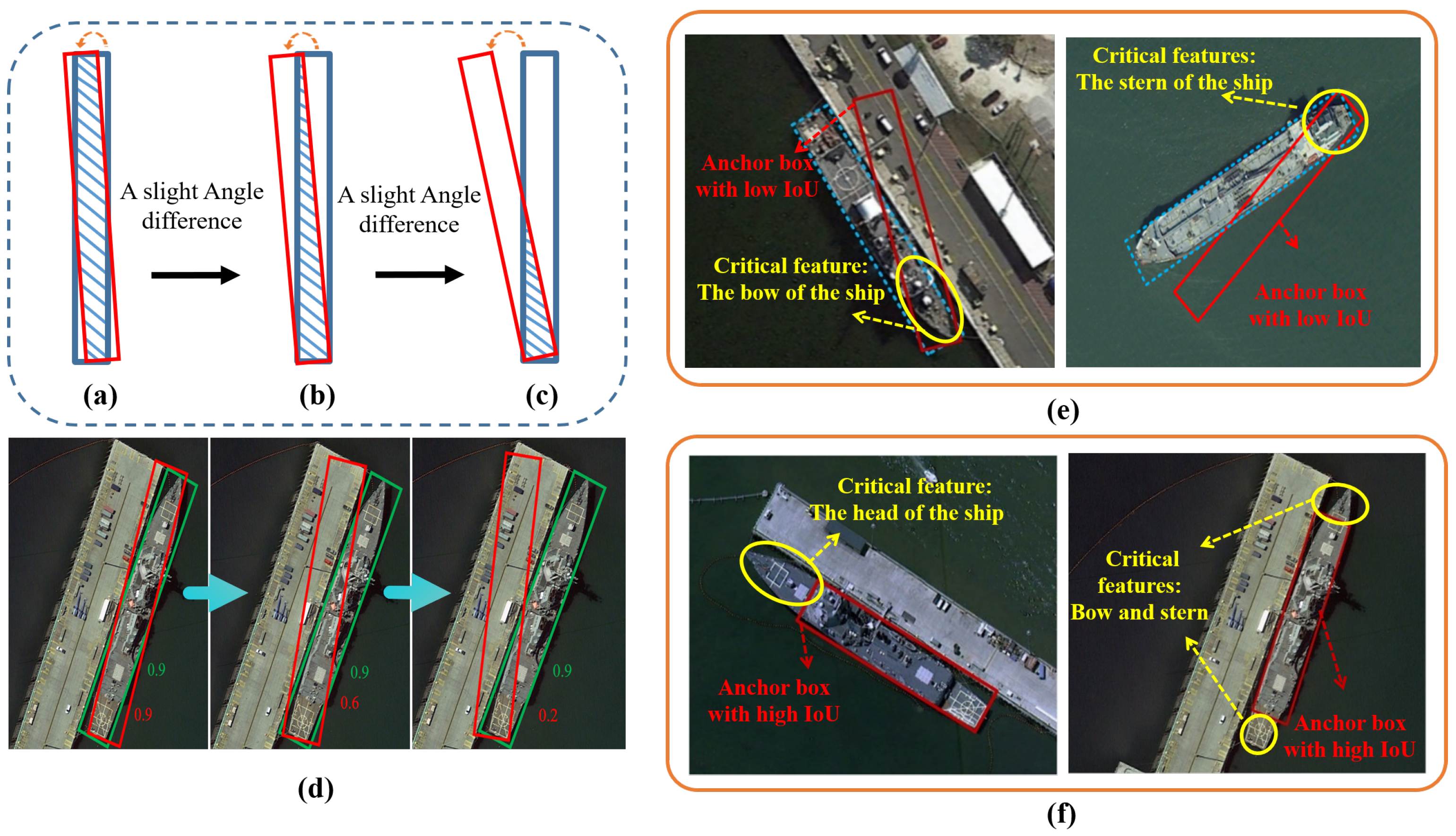
For targets with a large aspect ratio, such as some slender bridges, or ships with a length-to-width ratio greater than 10, even a very slight angle difference can lead to a significant decrease in the Intersection over Union (IoU) value, as shown in Figure 1a–d. Under the currently widely used five-parameter or eight-parameter bounding box representation methods, whether the bounding box can accurately capture the characteristics of elongated objects mainly depends on three core steps: (1) whether the learned pos/neg samples are representative, (2) whether the training strategy for matching the target is accurate and effective, and (3) whether the designed objective function is optimal. The combined influence of these factors determines the effectiveness and precision of the model in its bounding box representation.

Considering the above three important steps, we can summarize two major challenges for bounding boxes in accurately capturing the characteristics of slender objects: Firstly, in the sample selection stage, the label assignment with a fixed IoU threshold fails to adequately cover the critical information samples of slender targets, thereby limiting the model’s ability to learn crucial features of these targets. Secondly, in the target regression and loss function design stages, the complexity of the bounding box regression task for slender targets exceeds the general target, and the drastically changing loss function gradient leads to training instability. In the following sections, we will provide further elaboration on these two issues.

(1)

Missing high-quality sample boxes:

In RS object detection, relying solely on the IoU as an indicator to evaluate the accuracy of prediction boxes often fails to fully capture the critical characteristics of the target. Although the IoU is high, as shown in Figure 1e, the prediction box fails to accurately capture the critical parts of the target, such as the end of the ship, which are crucial for understanding the overall structure of the target. Moreover, a small localization bias can cause a significant decrease in the IoU value so the anchor box (red box of Figure 1f) containing keypoint information may be misclassified as negative samples or ignored. They limit the deep learning of the critical features of the target, which affects the detection accuracy of the model. In order to solve these problems, it is necessary to introduce a label assignment strategy that is more suitable for the elongated target shape.

(2)

Unstable training from sharp gradient changes in regression loss:

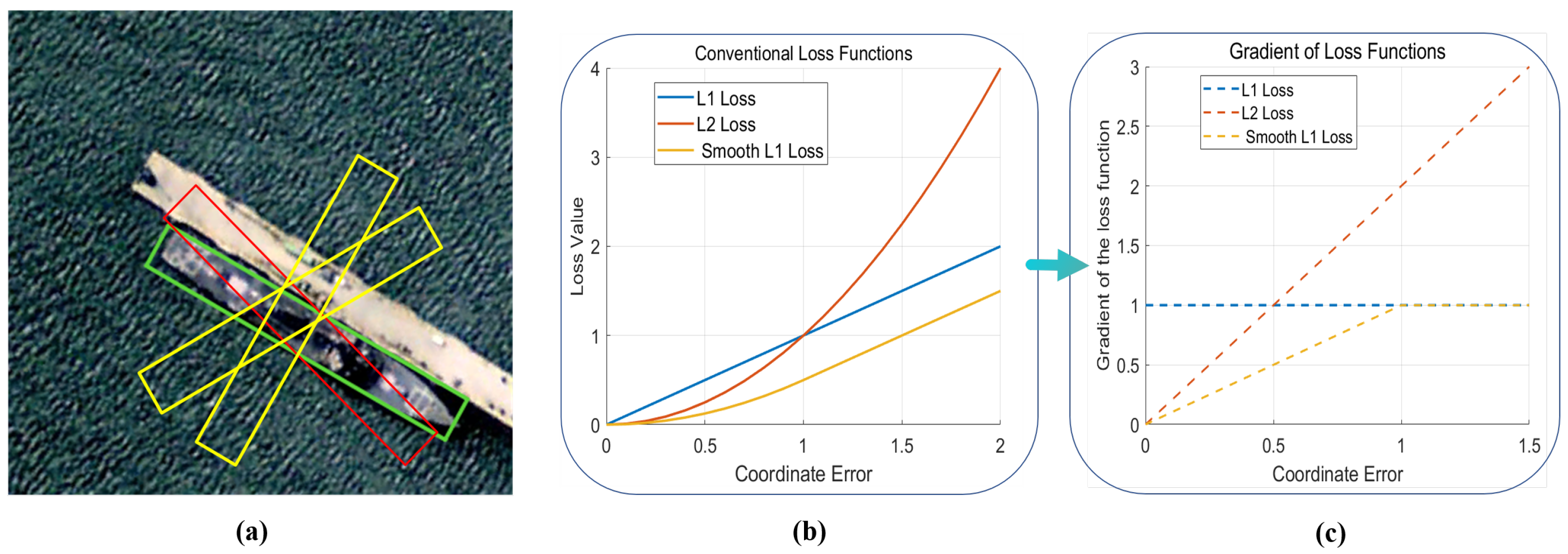
For slender RS objects, even small coordinate errors can easily lead to sharp increases in the gradient of the loss function, which requires that the loss function can sensitively capture these subtle changes. However, as illustrated in Figure 2b,c, many current loss function designs fail to encourage models to pay enough attention to these subtle errors. It makes it difficult to achieve accurate positioning of slender targets in the training process. Furthermore, during training, the model usually gives preference to those anchor boxes that yield large loss gradients, such as the one shown in Figure 2a that contains less information about the true target box (yellow box). These low-quality samples (yellow boxes) may mislead the model’s learning and often cause instability in regression training, resulting in a decrease in model performance. To overcome these challenges, we need to design a more accurate and stable training objective function.

In addition, we believe that an ideal bounding box representation should meet the following characteristics.

First of all, an accurate sampling strategy ensures that sufficient samples are provided for different-shaped objects, especially elongated targets, to enrich the critical information of the training data. Secondly, the evaluation criteria are effective for effective regression tasks. The designed evaluation index and loss function accurately reflect the bounding box regression performance in the detection of slender objects. Thirdly, to ensure efficient deployment, the detection head maintains accuracy while reducing the computational burden as much as possible, which requires concise algorithms.

To this end, we propose the ABP-Net for the detection of slender targets in RS images. ABP-Net focuses on enhancing the model’s boundary perception capabilities with two crucial modules.

Dynamic label assignment (S-S): This feature adjusts the IoU threshold dynamically for elongated targets, ensuring that positive samples include the most informative features. This adjustment is crucial for refining the model’s ability to detect boundaries accurately.

Robust loss function (R-R): The R-R loss function is designed to increase the model’s sensitivity to minor errors while ensuring stable training for targets with large aspect ratios. This function is essential for reliable model convergence.

Our main contributions are concisely outlined as follows:

(1)

The S-S module boosts detection accuracy by enhancing the model’s ability to adapt to elongated targets’ shapes and boundaries.

(2)

The R-R loss function’s advanced gradient management is critical for stable training on objects with complex boundaries.

(3)

ABP-Net outperforms state-of-the-art models on UCAS-AOD and HRSC2016 datasets, excelling in complex boundary detection for slender targets.

2. Related Works

The rule for assigning an anchor as a positive or negative example is called label assignment. Using appropriate label assignment can effectively improve the performance on the basis of a small inference cost, which is the core step that affects the performance of the model. In the following, it can be divided into two methods: fixed label assignment and dynamic label assignment.

2.1. Fixed Label Assignment

The classical object detectors employ a defined strategy to assign positive and negative samples. According to the presence or absence of an anchor, it can be divided into two methods: the anchor-based strategy and anchor-free detector strategy.

(1)

Anchor-based strategy:

Models such as Faster R-CNN [8], SSD [1], and RetinaNet [2] have traditionally employed fixed-threshold-based label assignment methods to distinguish between positive and negative samples. This approach initiates by defining a set of anchor boxes with various aspect ratios and sizes. For each ground truth bounding box, the IoU with all anchor boxes is calculated to determine the classification of the samples. If the IoU is greater than or equal to a predetermined threshold, the anchor box is considered a positive sample; otherwise, it is deemed negative. RFLA [15] first utilizes the prior knowledge that the feature receptive field follows a Gaussian distribution, proposing a new strategy based on the Receptive Field Distance (RFD). Furthermore, it also designs a Hierarchical Label Assignment (HLA) module based on RFD, which enhances the accuracy of positive and negative label assignments for detecting tiny objects.

(2)

Anchor-free strategy:

FCOS [16] employs a center sampling strategy which generates multiple anchor boxes of different scales centered on the ground truth (GT) box’s center. For each generated anchor box, it is assigned as a positive or negative sample based on its IoU between the real box and its category. Subsequently, the improved FoveaBox [17] adopts the Pyramid Fovea Pooling strategy, pooling the feature maps at multiple scales to obtain feature maps of different scales. Then, for each real box, the corresponding feature map is selected based on its scale. On the chosen feature map, multiple anchor boxes of different scales are generated centered on the real box’s center, and the generated anchor boxes are assigned as positive or negative samples by calculating their IoU with the real box. The scales of these anchor boxes correspond to the scales of the feature maps, which helps the model more accurately capture objects of various scales. Li et al. [18] introduced a new metric called Pseudo-IoU. First, for each predicted box, all IoU values with the real boxes are sorted, and then a certain proportion of the top IoU values corresponding to the real boxes is selected using the labels of these real boxes as pseudo labels for the predicted box. By improving the IoU, the predicted boxes learn more features of positive samples during training, alleviating the imbalance of sample distribution and improving detection accuracy.

Although simple, these fixed label assignments have drawbacks. They depend too much on the coordinates of the samples, do not consider the contextual features of the target, and lack adaptability.

2.2. Dynamic Label Assignment

In the last two years, an adaptive detector mechanism was proposed to improve label assignment which can automatically select positive and negative samples according to the statistical characteristics of the object with the aim of further improving the detection performance. FreeAnchor [19] constructs the top k highest anchor candidates based on the IoU of each object, and calculates the importance scores from the classification and localization confidence according to the Mean–Max function to achieve dynamic positive and negative assignment. ATSS [20] calculates the L2 distance between each sample point and the center point of the true box, retains the top k anchor points with the smallest distance, and uses the IoU of the mean + std of the top k anchor points of each GT group as the pos/neg threshold, and the IoU greater than the threshold is a positive sample. PAA [13] is a probabilistic anchor assignment method. Firstly, the CLS and REG joint loss distribution of positive samples and negative samples is assumed to obey Gaussian distribution, then the GMM is used to fit the distribution of pos/neg samples, and the positive and negative labels are assigned according to the probability deduced from it. However, the computational complexity of the PAA method is high, which may increase the training time, and the assignment effect is easily affected by the sample noise. The following year, Ma et al. [14] proposed IQDet in order to mitigate the impact of noisy samples and per-sample quality rules on dynamic rules such as PAA. IQDet is based on the GMM to better capture the distribution characteristics of objects, and also adopts the instance (GT-wise) sampling quality distribution to assign a unique label to each object. Even in the case of target overlap or contact, it can ensure the stability of the tag.

These dynamic methods take into account the environmental interaction of image features, and can adaptively obtain the corresponding best selection according to different feature target sets to a certain extent. However, there are also some limitations. For example, it is susceptible to sample noise, there is uneven distribution of sample quality, and, due to the complexity of environmental interaction, the network cannot provide accurate results for label assignment stably. Especially for the large-aspect-ratio target, it is difficult for these methods to capture the critical information according to the shape change and assign reasonable high-quality positive and negative samples.

3. Methodology

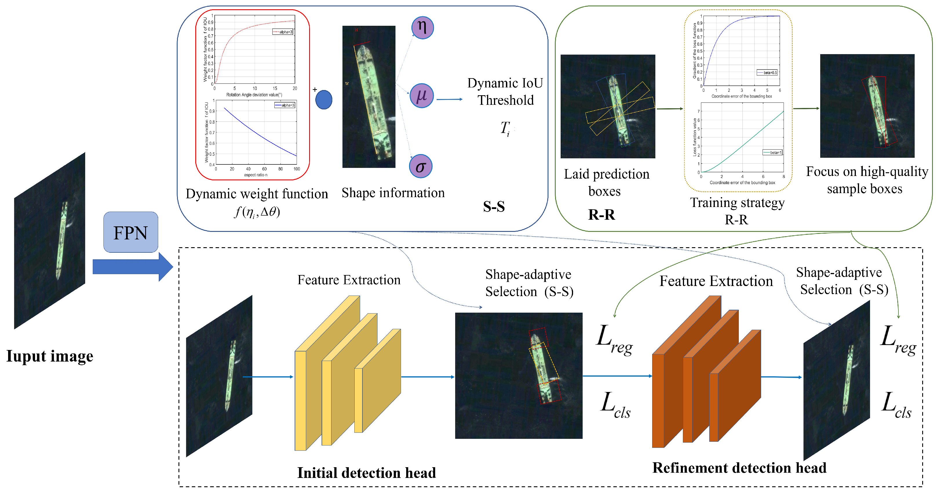
This section presents the methodology of ABP-Net, tailored for enhancing the detection of slender targets in remote sensing imagery. Section 3.1 introduces the Shape-Sensitive label assignment, which is pivotal for dynamically adjusting the IoU threshold to ensure that our model captures the critical features of slender targets effectively. Section 3.2 then emphasizes the Robust–Refined loss function, specifically designed to address the challenges posed by the elongated nature of slender targets. This function stabilizes the training process by focusing on low-error samples and suppressing the gradient amplification that typically affects difficult samples, thereby enhancing the model’s ability to accurately detect and localize slender objects. The complete framework of our ABP-Net is depicted in the accompanying Figure 3.

3.1. Shape-Sensitive Label Assignment (S-S)

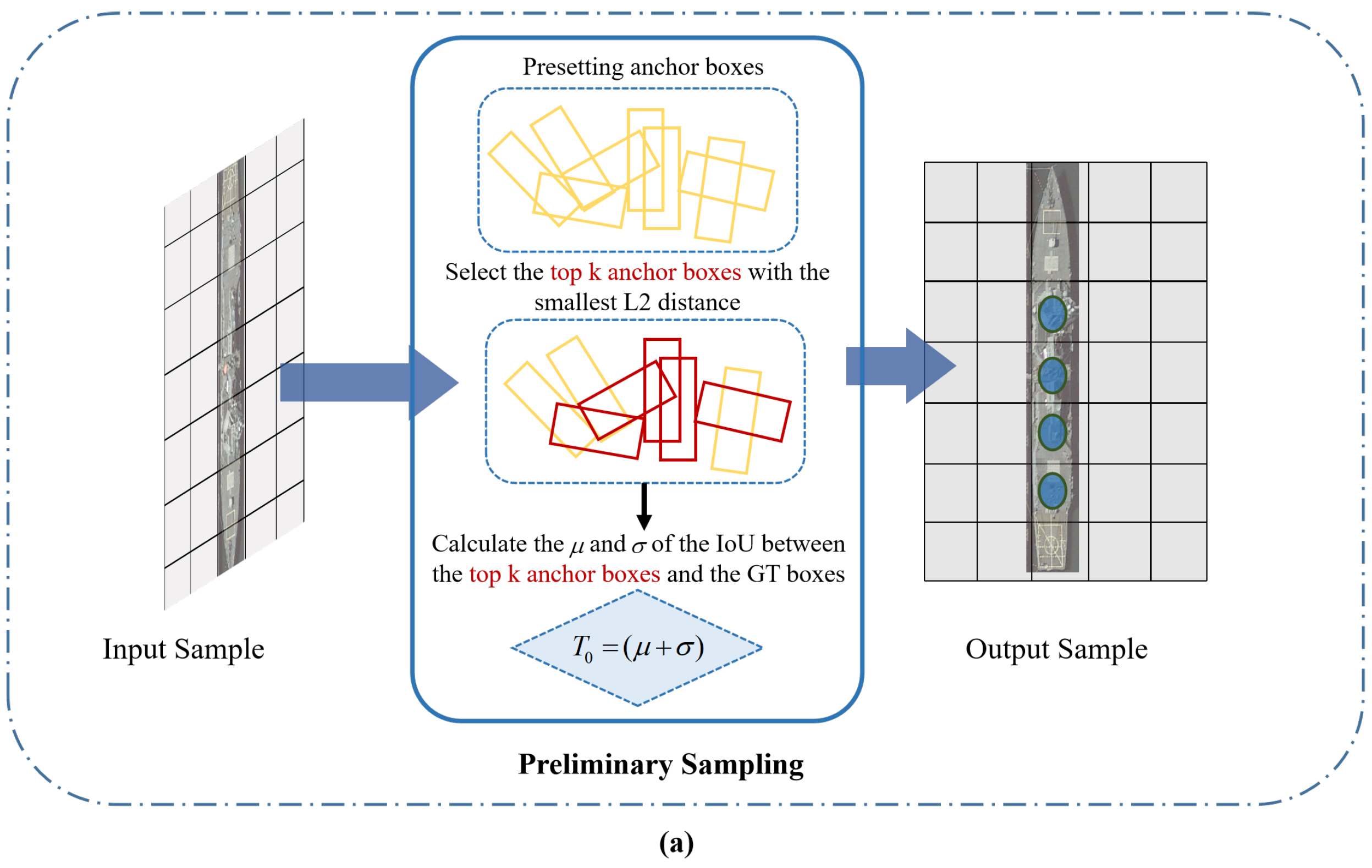
For the sample selection stage before training, targeting the problem where it is easy to miss the positive samples with critical information when dividing positive and negative samples for a high-aspect-ratio target, we design an adaptive adjustment label assignment. For the ground truth (GT) box i, the L2 distance between each of its preset anchor boxes and the center point of the GT box is calculated, the top k points with the minimum distance are retained to calculate the IoU of the preserved preset box and the GT box, and the mean $\mu$ and variance $\delta$ of this set of IoUs are calculated. The sum of the mean and variance $\mu +\sigma$ is used as the basic threshold and multiplied by the weight function $f({\eta }_i,\Delta \theta )$ to obtain the threshold $T_i$ for dividing positive and negative labels corresponding to the ground truth box i, and the expression is as follows:

$$\begin{array}{c}{\displaystyle \mu =\frac{1}{P}\sum _{j=1}^P{I}_{i,j},\sigma =\sqrt{{\displaystyle \frac{1}{P}\sum _{j=1}^P{(I_{i,j}-\mu )}^2}}}\\ \Delta \theta =|\theta -{\theta }_i|\\ T_i=f({\eta }_i,\Delta \theta )\ast (\mu +\sigma )\end{array}$$

(1)

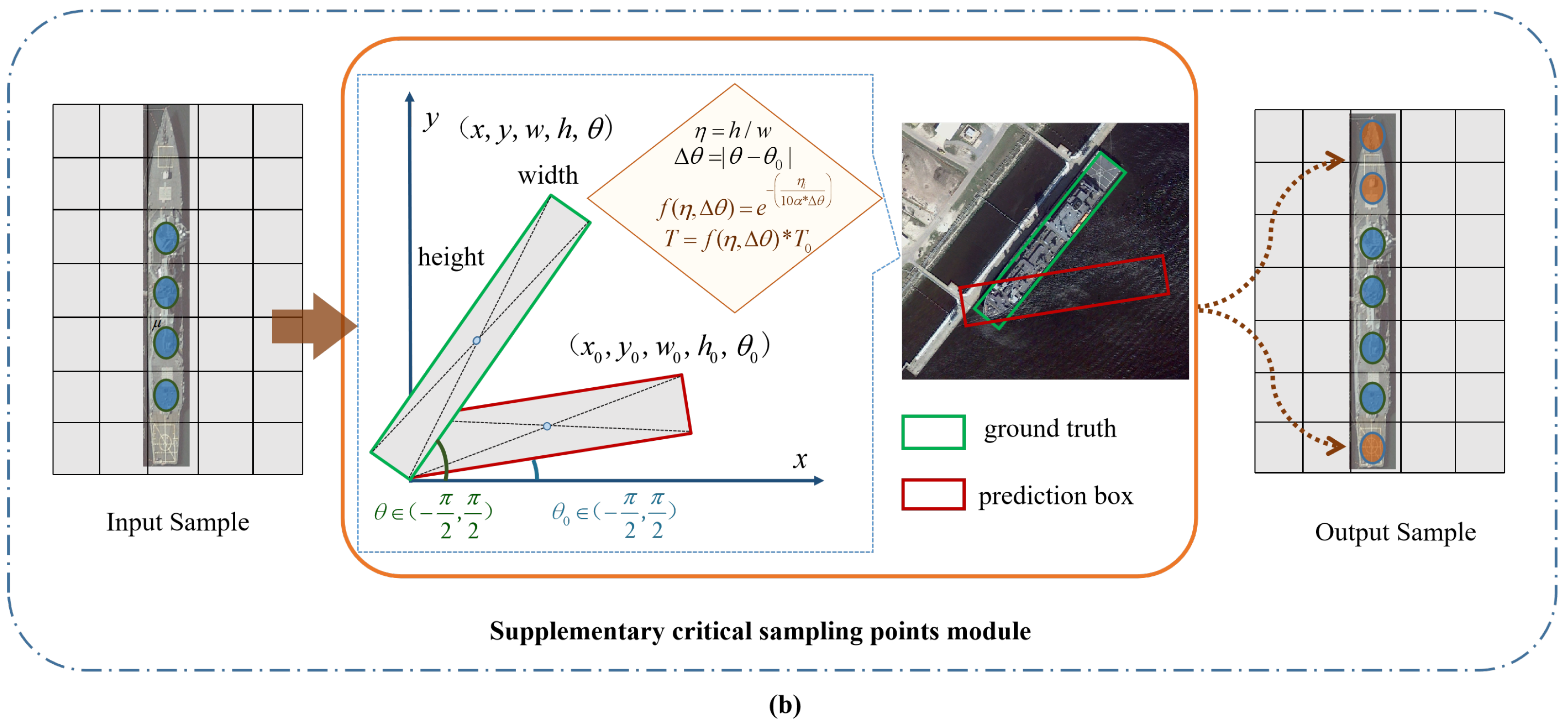
Among them, P represents the number of candidate anchor boxes, $I_{i,j}$ is the IoU ratio between the i-th true box and the j-th anchor box, $\theta$ is the angle between the anchor box and the horizontal axis, ${\eta }_i$ is the aspect ratio of the true box corresponding to the prediction, and $\Delta \theta$ is the difference between the angle between the horizontal axis of its preset box and the angle between the GT box and the horizontal axis.

In order to more adaptively divide the positive and negative samples of detection targets with different aspect ratios, a weight factor function $f(\eta ,\Delta \theta )$ determined by ${\eta }_i$ and $\Delta \theta$ is designed. The specific calculation formula is as follows:

$$\begin{array}{c}f({\eta }_i,\Delta \theta )=e^{-\left({\displaystyle \frac{{\eta }_i}{10\alpha \ast \Delta \theta }}\right)}\end{array}$$

(2)

$\alpha$ is the adjustable factor parameter of $\Delta \theta$. It can be seen from the previous format that the value domain of this function is [0, 1], which can be well adapted according to the different aspect ratio of the target, the angle difference of various sizes, and the dynamic reduction and increase in the threshold of IoU $T_i$ in the interval $[0,\mu +\sigma ]$. It means a sample with high-quality target information can be divided into positive samples.

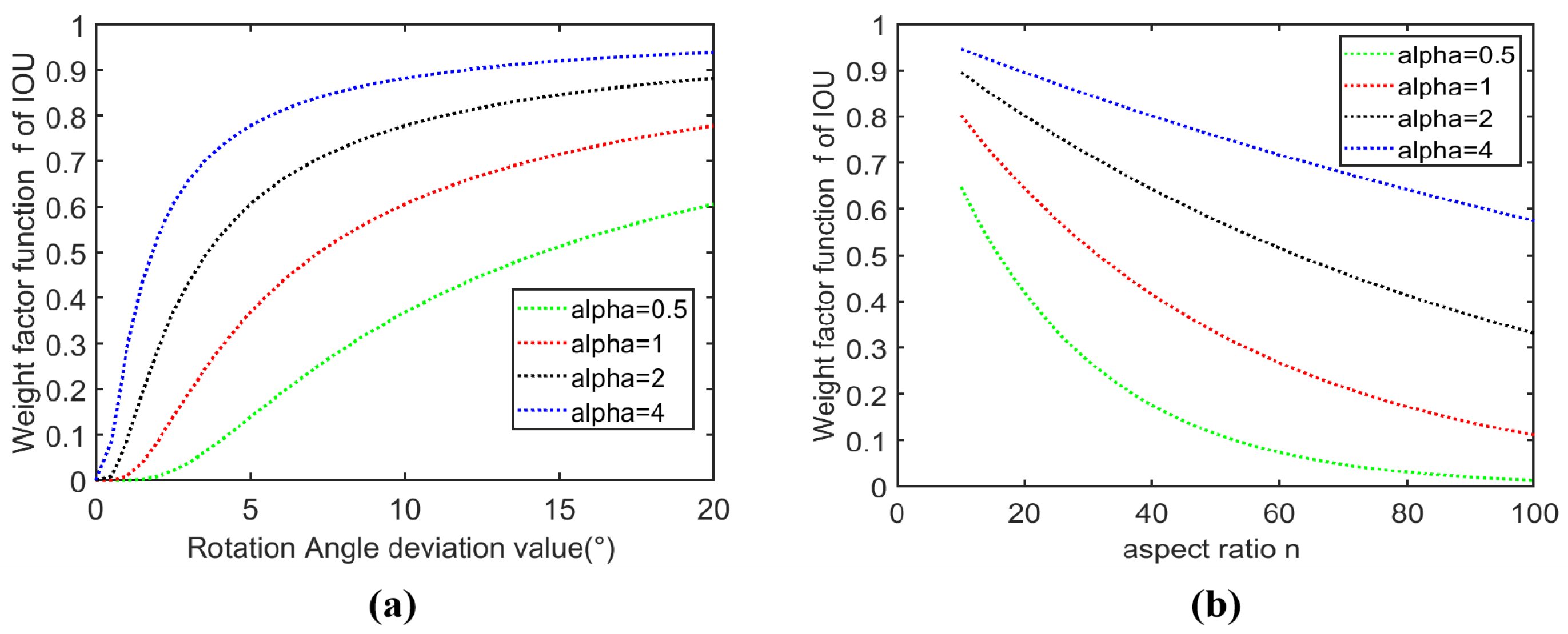
The trend of $f(\eta ,\Delta \theta )$ changes is shown in Figure 4. When the aspect ratio ${\eta }_i$ of the target increases and its corresponding $\Delta \theta$ is small, the weight factor $f({\eta }_i,\Delta \theta )$ will decrease. When the aspect ratio ${\eta }_i$ of the target is high but the angle difference $\Delta \theta$ increases, the threshold decline speed of the IoU value will decrease with the increase in $\Delta \theta$.

By setting a dynamic threshold, the S-S module can better capture the critical features of the target and mine the contribution of potential low-quality samples to the model. This is shown in Figure 5. First, we use $\mu +\sigma$ as the initial threshold $T_0$ to pick out good-quality samples from multiple anchor boxes laid in preparation for later dynamic adjustment of the threshold. Then, on the basis of the initially selected samples of good quality, the threshold is dynamically reduced or increased according to the aspect ratio of the target $\eta$ to further capture the critical characteristics of the elongated target, that is, the orange dots in the output samples.

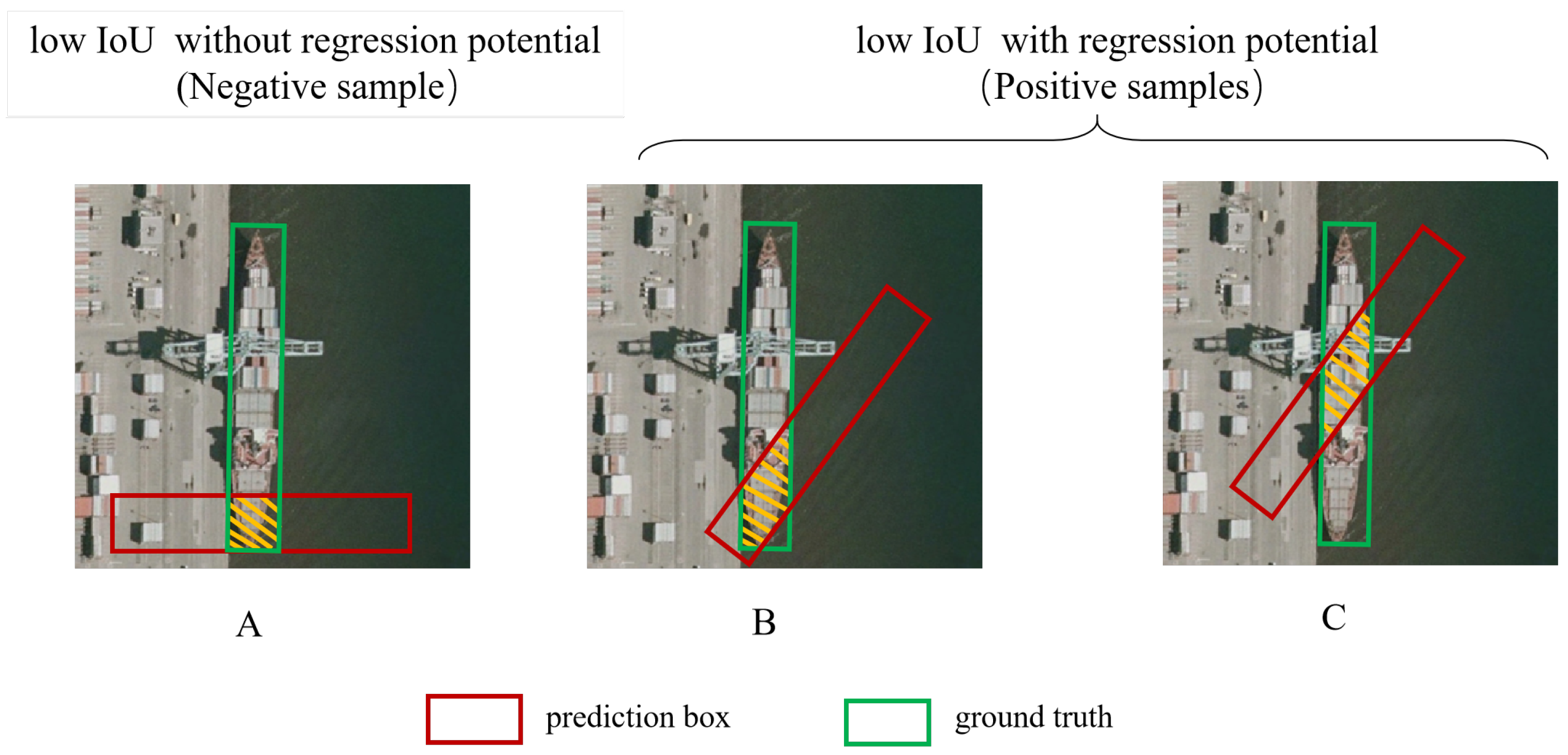
In contrast to directly lowering the threshold for elongated anchors, we prevent low-IoU, low-quality samples (As shown in Figure 6A) from being classified as positive samples by introducing the angle difference between GT boxes and predicted anchors $\Delta \theta$. We consider that, when the angle difference $\Delta \theta$ is very small, if the anchor box contains the features of both ends of the slender target, As shown in Figure 6B, it will make the model learn the slender target more fully. If the features at both ends are not included, such as in Figure 6C, this anchor box may also be a potentially high-quality sample that is easy to regress.

3.2. Robust–Refined Loss Function (R-R)

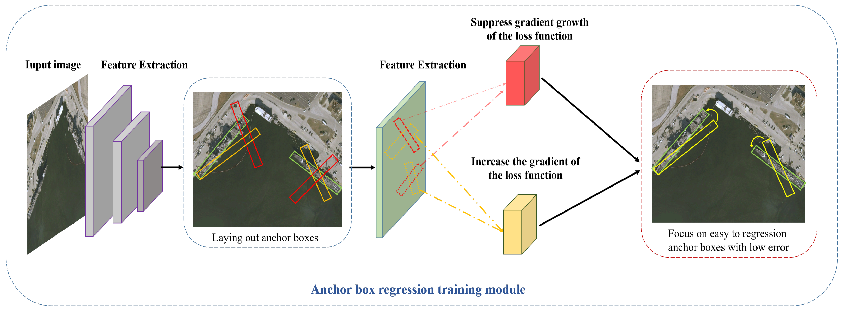
Although in the pre-training stage we classify the anchor boxes with regression potential as positive samples, in the later stage of anchor regression training, we also need to ensure that the model is able to focus on the low-error samples that are easy to regress.

The loss function of remote sensing target detection is a multi-task loss function, which is divided into classification loss and detection box regression loss as follows:

$$\begin{array}{c}{L}_{p,t,p_r,t_r}=L_{cls}(p,t)+\lambda [t⩾1]L_{reg}(p_r,t_r)\end{array}$$

(3)

In the classification loss function $L_{cls}$, p and t represent, respectively, the category predictive values and category tags of the network. In the regression loss function $L_{reg}$, $p_r$ and $t_r$ represent, respectively, the return result corresponding to the predicted classification results and the corresponding regression tags. $\lambda$ is used to adjust the weight of loss under multi-tasking learning.

In order to deal with the high length and width ratio of the anchor box and the GT box for the regression task, there is only a small angle difference for the real box. It will still cause its large gradient loss and the problems of unstable training and poor regression effects caused by the poor training. We design a gradient expression of a loss function. At the same time, the specific expression is shown below:

$$\begin{array}{c}{\displaystyle \frac{\partial L_{reg}}{\partial x}}=1-e^{-\beta x}\end{array}$$

(4)

Among them, for the error value of the regression, $\beta$ is the adjustable parameters. Observe the curve of the loss gradient function with the change in x. As shown in Figure 7a below, we increase the sample gradient growth rate of small errors, prompting the model to pay more attention to small error samples with rich accurate information and speed up the model convergence. At the same time, we inhibit the gradient ascension of the large error sample, that is, the loss gradient will not increase infinitely with the increase in the return error. Instead, the loss function accompanies the increasing regression error, and the increasing gradient is infinitely close to 1 to achieve more stable and more accurate training. Not only that, the value domain of the ladder of the loss function is not greater than 1, but it can also effectively prevent the gradient explosion. Among them, the value of the parameter $\beta$ is closely related to $\eta$. When the aspect ratio is higher than $\eta$, the gradient changes of the sample of small errors should be more severe, and $\beta$ will become larger.

The integral can be obtained to obtain the loss function expression as follows:

$$\begin{array}{c}{L}_{reg}=x+{\displaystyle \frac{1}{\beta }}{e}^{-\beta x}+C,x⩾0,C\mathrm{is}\mathrm{a}\mathrm{constant}\end{array}$$

(5)

When x = 0, $L_{reg}$ is also 0, and the value of the constant C can be calculated as follows:

$$\begin{array}{c}\left\{\begin{array}{c}x+{\displaystyle \frac{1}{\beta }}{e}^{-\beta x}+C=0\\ x=0\end{array}\right.,C={\displaystyle \frac{1}{\beta }}\end{array}$$

(6)

That is, the final R-R loss function is

$$\begin{array}{c}{L}_{reg}=x+{\displaystyle \frac{1}{\beta }}{e}^{-\beta x}-{\displaystyle \frac{1}{\beta }},x⩾0\end{array}$$

(7)

We present a schematic of our R-R anchor regression training module in Figure 8. This module strategically modulates the gradient of the loss function, with a focus on enhancing the model’s attention to low-error anchor boxes conducive to regression, as indicated by the yellow blocks. Conversely, the red blocks signify areas where the gradient growth is suppressed, thereby optimizing the model’s learning process.

4. Experiments

The experimental results are presented for two typical public datasets containing targeted objects: HRSC2016 (Liu et al., 2017) [21] and UCAS-AOD (Zhu et al., 2015) [22]. Details regarding the datasets, method implementation, evaluation metrics, and experimental outcomes are discussed in the subsequent subsections.

4.1. Datasets

4.1.1. HRSC2016 Dataset

The HRSC2016 dataset, introduced by Liu et al. in 2017 [21], is a high-resolution satellite image dataset dedicated to ship detection. It comprises 436 images for training the model, 181 images for validating its performance, and 444 images for the final testing phase. The images vary in size, from as small as 300 × 300 pixels to as large as 1500 × 900 pixels, encompassing a range of ship sizes. To ensure consistency, all images are resized to a standard resolution of 800 × 512 pixels for both training and testing.Ship images within the HRSC2016 dataset feature arbitrary aspect ratios and orientations, offering rich variations and posing challenges for detection algorithms. The dataset is characterized by a diverse distribution of targets, including various types, sizes, and colors of ships, as well as ships in diverse maritime environments. The images frequently include complex backgrounds such as waves, clouds, and coastlines, which further complicate the ship detection task.

4.1.2. UCAS-AOD Dataset

The UCAS-AOD dataset (Zhu et al., 2015) [22] is an aerial photography dataset for aerial object detection with a focus on the detection of cars and airplanes. This dataset contains approximately 1510 images with a total pixel size of about 659 × 1280 pixels and a total of 14,596 labeled instances. The images display a variety of car and aircraft types and their appearances under different environmental conditions, such as varying lighting, weather, and seasonal changes. In this study, 1057 images are randomly selected from the UCAS-AOD dataset for training purposes, while 302 images are used for testing. The dataset features a diverse distribution of targets, including cars and aircraft of various models, colors, and sizes, as well as their distribution across various settings, such as airport runways, parking lots, and city streets. The images of the UCAS-AOD dataset are of high quality and are accurately annotated, providing a valuable resource for research in car and airplane detection.

4.2. Implementation Details

In our research, we established two baseline models: one based on the anchor point using the main network of ResNet101 [23] and the other utilizing the anchor-free method of RepPoints [24]. Both methods employ a main network for feature extraction and are equipped with two detection heads to refine the prediction results. We selected the Feature Pyramid Network (FPN) [25], as introduced by Lin et al. in 2017, combined with ResNet101 [23], as detailed by He et al. in 2016, to form the main trunk of our models. During training, we used the SGD (stochastic gradient descent) optimizer, setting the initial learning rate, momentum, and weight decay to 0.012, 0.9, and 0.0001, respectively.

To evaluate the optimal training duration, we trained our model using 36, 96, 120, and 240 epochs on both the HRSC2016 and UCAS-AOD datasets. Our findings indicate that 120 epochs is the most effective training period, offering a balance between model accuracy and computational demand. The 36-epoch training is too brief for the model to achieve adequate accuracy levels. At 96 epochs, the model showed signs of improvement but with some inconsistencies in performance. Extending to 120 epochs, we observed a refinement in the model’s predictive capabilities, aligning with our goal of enhancing model convergence without overfitting. This period yielded the highest mAP scores on our validation datasets, demonstrating a robust and stable performance. Importantly, while doubling the training duration to 240 epochs might have been expected to further improve performance, our results indicated no significant gains in accuracy. Instead, we noted a plateau in performance, suggesting that the model had already reached its convergence potential at 120 epochs. Furthermore, the extended training period increased computational costs without commensurate benefits in detection accuracy. Therefore, we selected 120 epochs as the standard training duration for our experiments as it provided the most efficient and effective training outcome. The entire training process for UCAS-AOD and HRSC2016 took approximately 1.7 h and 3 h, respectively.

In the anchor-free RepPoints model, we set the number of points to 12, and, in the anchor-based ResNet-101 model, we set the number of anchor points at each position to 1. The weighted parameter $\omega$ was adjusted based on experimental experience with the two datasets. Additionally, the experiments utilized the MMDETECTION 1.1 framework [26] and PyTorch 1.3, along with the MMrotate framework, with 11 G of memory and six GPUs with 62 G of memory each. Each experiment was performed more than twice, and the average value was taken as the final result. Our data augmentation strategy included random flipping and random rotation. The benchmarks presented in

Table 1. The results of ablation experiments using anchor-free RepPoints as the backbone network are presented for the UCAS-AOD and HRSC2016 datasets.

Dataset	S-S	R-R	mAP (%)
UCAS-AOD	✗	✗	84.59
	✓	✗	88.72
	✓	✓	89.80
HRSC2016	✗	✗	76.01
	✓	✗	81.78
	✓	✓	85.01

,

Table 2. The ablation results of the UCAS-AOD and HRSC2016 datasets using the anchored ResNet-101 as the backbone network are presented.

Dataset	S-S	R-R	mAP (%)
UCAS-AOD	✗	✗	86.12
	✓	✗	88.05
	✓	✓	90.02
HRSC2016	✗	✗	85.22
	✓	✗	87.92
	✓	✓	90.17

,

Table 3. Performance comparison of S-S strategy with other label assignment on HRSC2016.

Based Method	Sample Selection	mAP (%)
RepPoints (anchor free)	FreeAnchor	69.12
	MaxIoU	74.95
	ATSS	75.93
	S-S	81.78
ResNet101 (anchor based)	FreeAnchor	78.82
	MaxIoU	81.36
	ATSS	87.05
	S-S	87.92

,

Table 4. Performance comparison of our R-R strategy with other boundary box regression loss function on HRSC2016.

Based Method	Regression Loss Function	mAP (%)
RepPoints (anchor free)	L1 loss	79.21
	L2 loss	78.83
	Smooth loss	81.78
	R-R	85.01
ResNet101 (anchor free)	L1 loss	82.91
	L2 loss	82.64
	Smooth loss	87.92
	R-R	90.17

,

Table 5. Results of sensitivity experiments on parameter $\alpha$.

$\mathit{\alpha }$	0.5	1	2	3	4	5
mAP	87.18	88.35	88.94	89.03	88.98	87.90

and

Table 6. Results of sensitivity experiments on parameter $\beta$.

$\mathit{\beta }$	0.5	1	5	10	15	20
mAP	89.14	89.62	89.86	90.14	90.29	90.18

and the experimental results of our methods were compared fairly with other methods through multi-scale training and data augmentation, as shown in

Table 7. Comparison of the impact of various rotation methods on the HRSC2016 dataset. We tested the FPS in an environment with a single NVIDIA GeForce RTX 2080 Ti GPU, which has 11 GB of video memory, and calculated the FPS by dividing the total inference time by the number of chip images.

Method	Backbone	mAP	FPS
RDD (Liao et al. 2018)  [27]	VGG16	83.98	-
RoI-Transformer (Ding et al. 2019) [11]	ResNet101	85.09	7.4
Gliding Vertex (Xu et al. 2020) [12]	ResNet101	87.91	10.2
CSL (Yang and Yan 2020) [28]	ResNet101	88.86	-
RSDet (Qian et al. 2021) [29]	ResNet101	86.64	9.8
BBAVec (Yi et al. 2021) [30]	ResNet101	88.21	-
R3 Det (Yang et al. 2021) [31]	ResNet101	89.05	-
DAL (Ming et al. 2021) [32]	ResNet101	89.25	-
Anchor free:
RepPoints [24]	ResNet101	78.61	11.6
Ours	ResNet101	85.06	13.1
Anchor based:
S2ANet [33]	ResNet101	90.10	14.3
Ours	ResNet101	90.29	14.7

and

Table 8. Comparison of mAP with state-of-the-art methods on UCAS-AOD.

Method	Car	Airplane	mAP
YOLOv3 (Redmon and Farhadi 2018) [5]	73.90	89.20	81.55
RetinaNet (Lin et al. 2017) [2]	85.37	87.62	86.50
Faster-RCNN (Ren et al. 2015) [8]	86.41	89.73	88.07
RoI-Transformer (Ding et al. 2019) [11]	88.11	89.92	89.02
RIDet-Q (Ming et al. 2021) [34]	88.76	89.88	89.32
RIDet-O (Ming et al. 2021) [34]	89.11	90.24	89.68
DAL (Ming et al. 2021) [32]	89.05	90.17	89.61
Anchor free:
RepPoints [24]	84.76	89.01	86.88
Us	89.52	90.20	89.85
Anchor based:
S2ANet [33]	88.97	90.51	89.74
Us	89.67	90.51	90.09

.

4.3. Ablation Studies

4.3.1. Evaluation of Different Components

We conducted ablation experiments on the HRSC2016 and UCAS-AOD datasets to verify the performance of the different modules we proposed. To ensure the reliability of our results, we performed each ablation experiment three times and took the average of these trials. Table 1 lists the results obtained for each of these two datasets. Due to the difficulty in detecting critical features of targets with large vertical and horizontal ratios, the baseline models only achieved mAP scores of 84.59% and 76.01%, respectively. When employing the S-S module, the detector’s performance was optimized by 4.14% and 5.77%. This improvement indicates that the dynamic weight function of the S-S strategy ($\alpha$ = 1) can adaptively lower the IoU threshold according to the shape of the target. As a result, high-quality samples participate more effectively in model training, leading to a more comprehensive model that fully considers the critical features of the targets and enhances detection performance. In Table 3, we provide a comparison with other label assignment methods applied to the classic large-aspect-ratio dataset HRSC2016. The S-S strategy has a significant improvement compared with MaxIoU and ATSS, which further illustrates the ability of the S-S strategy to improve the detection accuracy of the target with aspect ratio.

Furthermore, we introduced the R-R loss function ($\beta$ = 10), which enhances the model’s sensitivity to fine-error samples by finely adjusting the gradient. This function also suppresses excessive attention to difficult samples, thereby effectively stabilizing the model’s gradient during the training process. As shown in Table 1, this strategy further promoted performance improvement, as evidenced by the increase in the mAP of 1.08% and 3.32% on the two datasets, respectively. Based on the S-S strategy, we compared the R-R strategy with three regression loss functions: the L1 loss function, L2 loss function, and smooth loss. As shown in Table 4, the R-R strategy performed best among the four methods on HRSC2016, both for the anchor-free method and in the anchor-free method.

In addition, we also conducted ablation experiments based on the model with anchor points (shown in Table 2), and also achieved similar performance improvements on the two datasets. The results of these experiments fully proved the effectiveness of our strategies in improving the performance of target detection, especially when dealing with challenging large-vertical-ratio targets.

Compared with only one module, different modules achieve better performance. Without the introduction of complex calculations, the participation of the S-S module and the R-R module gives the model training with rich critical features and high-efficiency and accurate regression guidance, thereby obtaining better regression and classification results. At the same time, the experiments also showed no conflict between the modules proposed. When an anchored ResNet-101 was used as the main network, the model showed the best performance of 90.02 and 90.17% mAP.

4.3.2. Evaluation of Parameters Inside Modules

For HRSC2016, based on the ResNet-101 backbone network with anchor points, we set up a parameter $\alpha$ sensitivity experiment to test the impact of the S-S module on model performance when the S-S module was added alone.

From Table 5, it is evident that, when $\alpha$ is less than 3, the smaller the value of $\alpha$, the lower the mAP. This suggests that the angle difference between the anchor frame and the real frame, particularly when $\alpha$ = 0.5 and $\alpha$ = 1, results in an undesirably low IoU value for targets with high vertical and horizontal aspects. This can lead to the inclusion of redundant information within the positive samples, which may contain irrelevant details. During training, the model is then tasked with extracting critical features from these potentially redundant positive samples, which significantly increases the computational burden and may limit the model’s learning efficiency and its ultimate detection accuracy.

When $\alpha$ exceeds 3, an increase in $\alpha$ correlates with a decrease in mAP. For instance, when $\alpha$ = 4 and $\alpha$ = 5, the IoU threshold may be overly suppressed, leading to the exclusion of some samples from the positive set even when they contain critical features of the target. This over-suppression can prevent the model from learning the essential characteristics of the target, thereby negatively impacting detection performance.

However, an $\alpha$ value of 3 achieves an mAP of 89.03%, indicating that the S-S strategy is well suited to the shape of the target and effectively learns its characteristics. In this scenario, the dynamic adjustment mechanism of the weight function may have found a balance point, avoiding both the over-suppression of high-quality samples with significant angle differences and the misclassification of low-quality samples as positive.

Additionally, we conducted a sensitivity experiment with the parameter $\beta$ to assess the impact of the R-R module on model performance when the S-S strategy is employed with $\alpha$ = 3. The results of this sensitivity analysis of the parameter $\beta$ are presented in Table 6.

We can observe that, when $\beta$ is less than 15, the mAP value decreases as $\beta$ decreases. This suggests that, for slender objects, such as those in the HRSC2016 dataset, settings of $\beta$ = 0.5, $\beta$ = 1, $\beta$ = 5, and $\beta$ = 10 do not effectively capture the aspect ratio characteristics relative to the number of coordinate errors, and the loss function may decrease too rapidly. Such configurations could lead the model to focus excessively on less important samples, thereby constraining the model’s detection accuracy. Conversely, when $\beta$ exceeds 15, particularly at $\beta$ = 20, the mAP decreases as $\beta$ increases. This trend indicates that the gradient of the loss function stabilizes prematurely at around 1, which restricts the model’s learning to the specific sample. Consequently, the model may fail to learn from sample boxes containing a wealth of information, which can result in diminished generalization capabilities.

In short, when $\beta$ = 15, the mAP reaches the peak of 90.29%, which indicates that, on the HRSC2016 dataset, the regression strategy and gradient settings of the model reached a proper balance. In this case, the model can effectively learn the critical low-error samples of the target, and, at the same time, avoid excessive attention to unimportant samples, thereby achieving precise testing of long-term ship targets.

4.4. Comparisons with State-of-the-Art Detectors

4.4.1. Results on HRSC2016

On the HRSC2016 dataset, our model achieved remarkable results in the remote sensing target detection task. This dataset includes a variety of ship types, moored in ports and oceans, providing a rich set of test scenarios for our methods. To ensure the reliability of our results, we conducted the experiments five times and took the average of these trials. By incorporating an innovative module, our approach achieved a 90.29% mAP score, surpassing the performance of the other existing detectors listed in Table 7. It is particularly noteworthy that our anchor-based ABP-Net demonstrated superior efficiency in specific ship detection. Compared to the $R^3 Det$ method, our model showed a 1.24% improvement in mAP, highlighting the efficiency of our approach.

In terms of performance comparison, in addition to mAP, FPS (Frames Per Second) is also an important metric which measures the real-time processing ability of the model. According to Table 7, our model also performed the best in FPS, achieving 14.7 FPS. Compared to RepPoints’ 11.6 FPS, our model was 3.1 FPS faster. The FPS of S2ANet was 14.3 FPS, which is slightly lower compared to our model, but our model still achieved a boost of 0.4 FPS. This shows that our model has a significant advantage in processing speed, and is able to complete the analysis and object detection of images faster under both anchorless and anchored frameworks, which is crucial for real-time monitoring and fast decision-making.

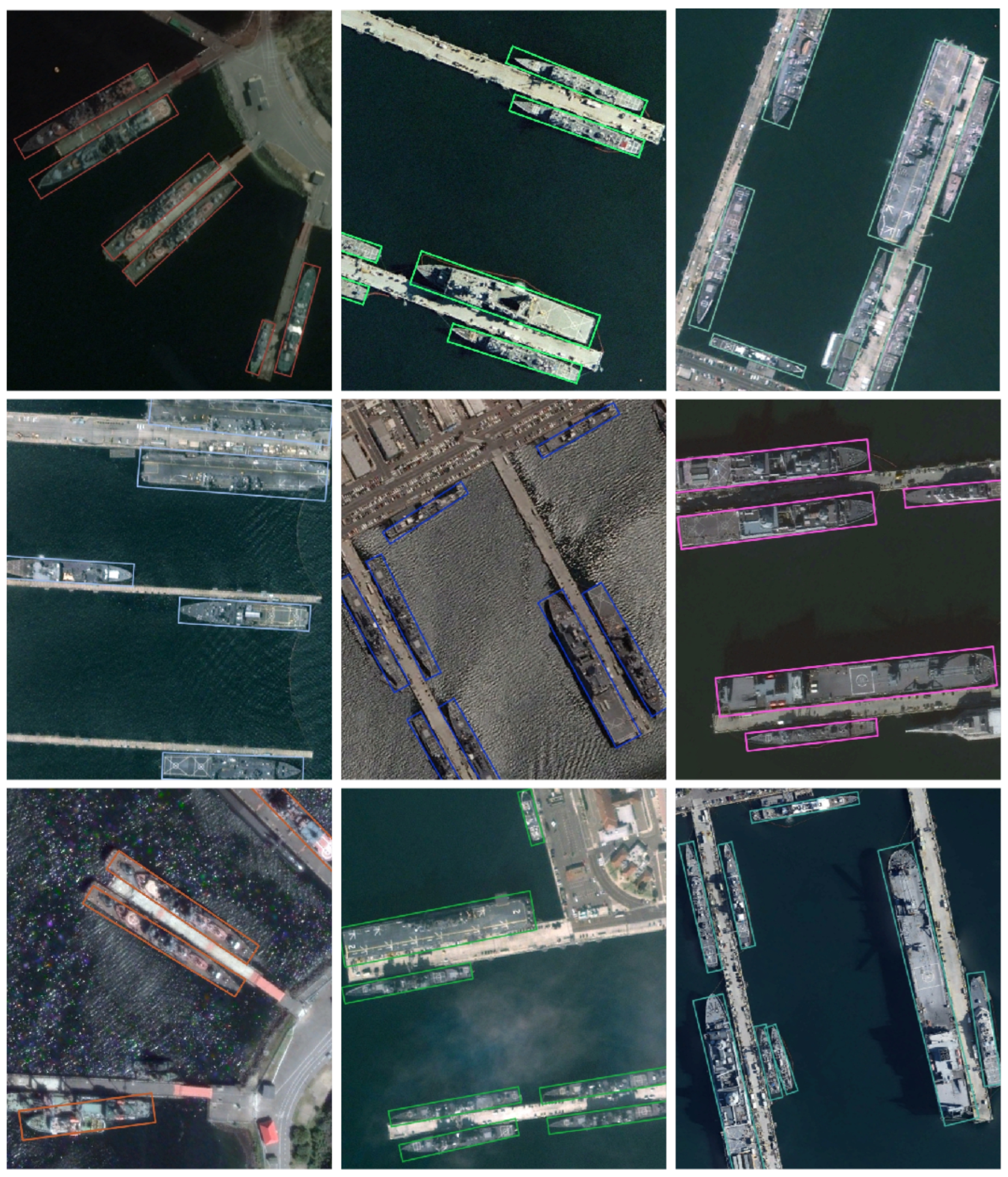
The visual detection results depicted in Figure 9 showcase our model’s excellent performance when dealing with diverse angle distributions, especially in complex scenarios such as docks or ports, where targets are densely clustered. These scenarios pose significant challenges for traditional target detection algorithms, which often struggle with missed detections or inaccurately locating slender targets due to unstable training. However, our model’s detection header employs an R-R regression training strategy that finely adjusts the gradient, significantly enhancing the model’s positioning accuracy on slender targets and effectively addressing these issues.

The third column of images in Figure 9 further confirms our model’s adaptability when targets exhibit greatly varying shapes and scales. In these images, the length of the ships varies significantly, with some differing by up to a factor of 10 in length. Our model employs the S-S strategy to fully learn the critical features of ships, enabling it to adapt and accurately position ships of various sizes. This not only demonstrates the model’s efficient positioning ability in target detection but also highlights its generalization capability when handling a diverse range of targets.

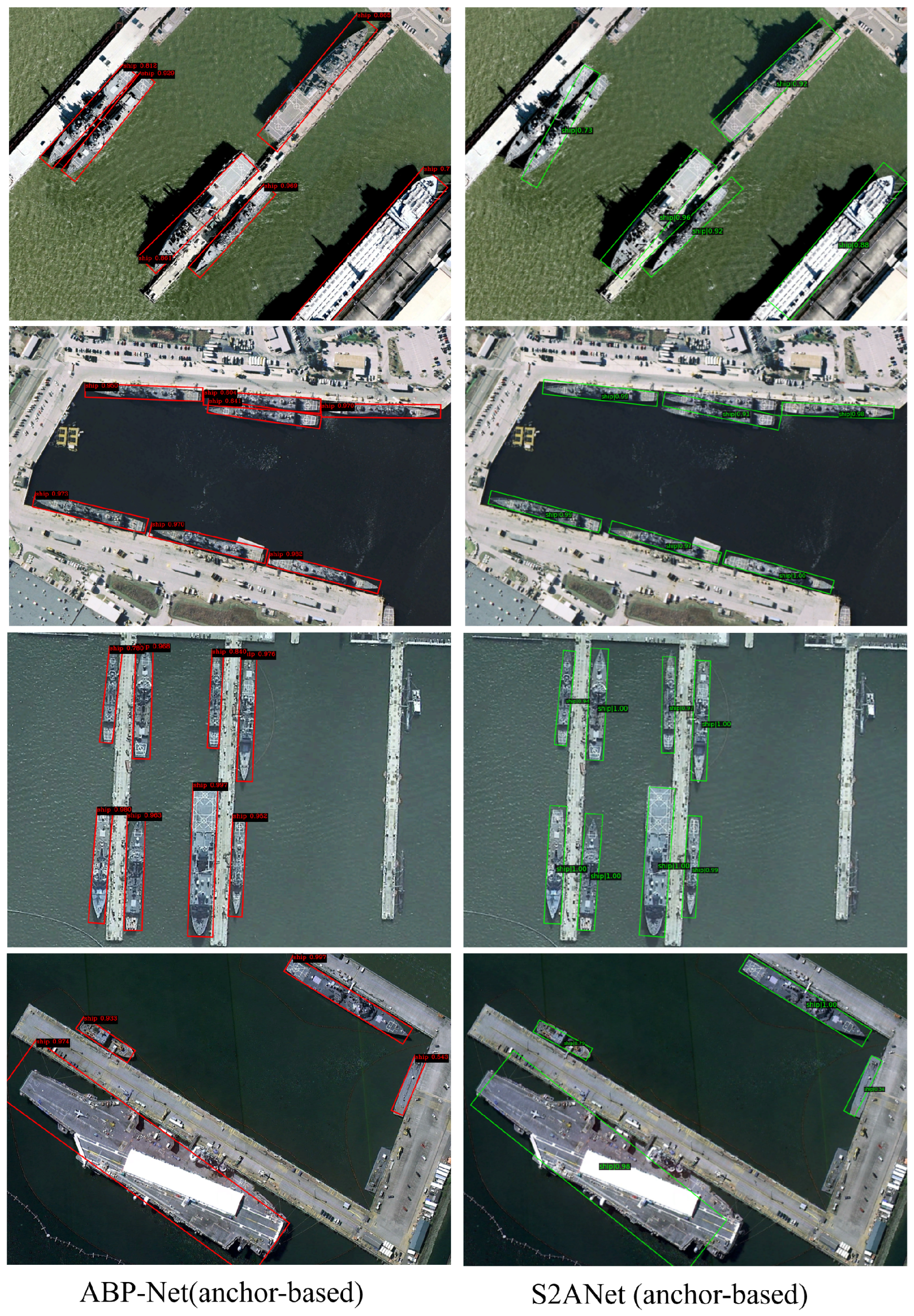
Moreover, Figure 10 provides a comparative analysis between our ABP-Net and the S2ANet on the HRSC2016 dataset. The first row of Figure 10 highlights the detection of densely packed ships. This underscores ABP-Net’s ability to resolve individual targets effectively, whereas S2ANet struggles with differentiation, leading to occasional merged detections. The second row of Figure 10 presents a comparison for harbor scenes with complex backgrounds. ABP-Net, with its S-S strategy and R-R regression training strategy, delivers more accurate bounding boxes that closely adhere to the ship contours, whereas S2ANet exhibits slight discrepancies, particularly in cases where ships are closely adjacent to the harbor or the other ship. For the third row of images, depicting densely packed ships, ABP-Net maintains a consistent level of precision, while S2ANet shows a slight decline in performance for ships with low contrast against the sea surface. The last row illustrates the scenario where there is a disparity in the scale of the targets. In such cases, the ABP-Net maintains a consistent level of precision, demonstrating its robustness across various target sizes. On the other hand, S2ANet experiences a noticeable decline in accuracy.

4.4.2. Results on UCAS-AOD

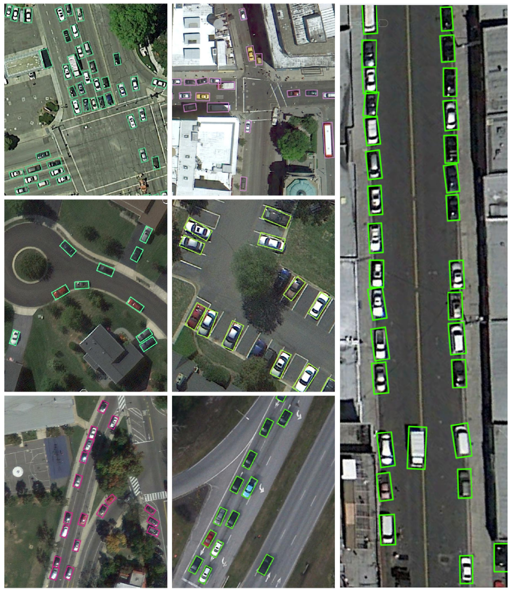
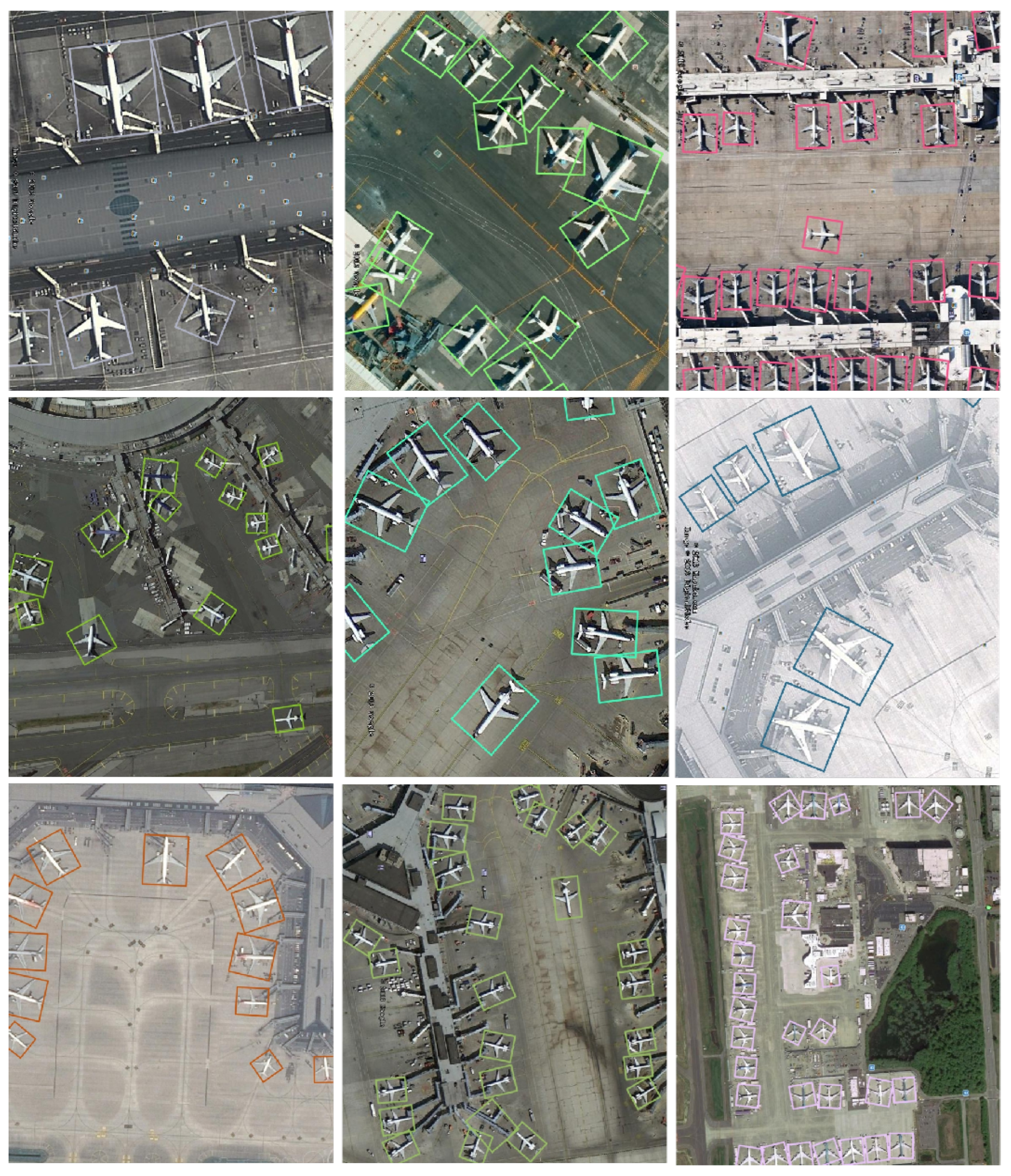
In the detection task on the UCAS-AOD dataset, our model exceeded existing technology with an mAP score of 90.09%, surpassing both secondary and primary detectors (shown in Table 8). Visualization results (as shown in Figure 11 and Figure 12) further confirm the model’s excellent performance when dealing with targets of varying aspect ratios. Within the dataset, the aspect ratio of most targets, such as vehicles and aircraft, is 1 or 1.5 times, yet our model can still accurately locate these targets. This is thanks to the S-S (Sample-Specific) strategy, which demonstrates outstanding adaptability and generalization for targets of different vertical and horizontal ratios by dynamically learning the target characteristics through an adaptive weighting function.

It is particularly worth mentioning that, in the densely packed aircraft scene depicted in the second column of Figure 12, where the noses of aircraft are interwoven with the fuselages of other aircraft, our model can still achieve effective positioning of each target. This accomplishment is attributed to the precise learning of critical target information, such as the heads and tails of the aircraft, by the S-S strategy. Meanwhile, traditional methods often struggle to achieve effective positioning due to unstable training gradients that are distributed in various orientations. Our R-R (Robust–Refined) regression strategy provides a more stable and accurate update direction for the model during the training process, significantly improving the positioning accuracy of the bounding box.

These results not only prove the efficiency of our model in the target detection task but also showcase its strong adaptability and generalization ability when handling complex scenes, all without significantly increasing computational complexity.

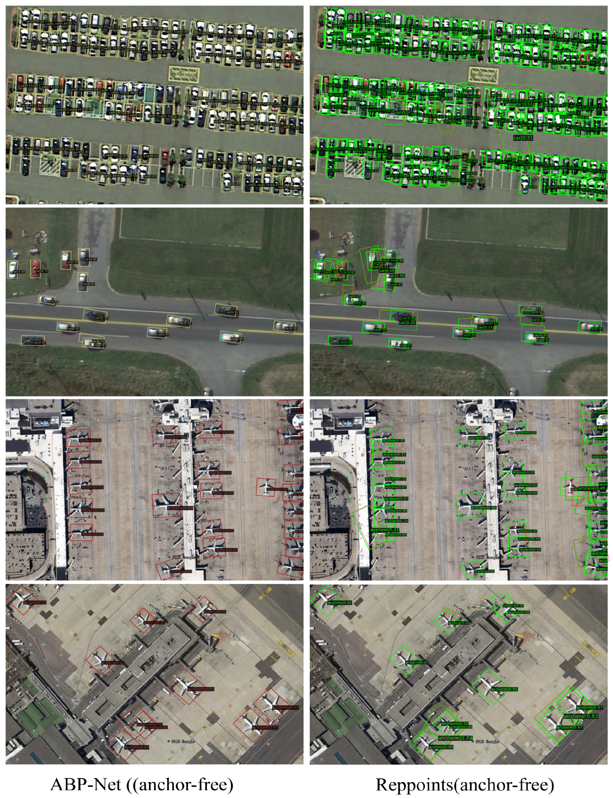
Furthermore, Figure 13 provides a comparative analysis between ABP-Net and the RepPoints method on the UCAS-AOD dataset, which includes cars and airplanes. The first and second row illustrates the detection of vehicles in urban environments. ABP-Net demonstrates superior accuracy in identifying cars, even under challenging conditions such as shadows and parked clusters. In contrast, RepPoints occasionally falters, producing less precise bounding boxes and missing smaller vehicles. The third and fourth row of Figure 13 focus on airplane detection, where ABP-Net excels in accurately pinpointing individual aircraft, regardless of their spatial arrangement or orientation. RepPoints, while performing adequately, shows a tendency to overfit bounding boxes, giving false alarms and overly large bounding boxes in scenes with high-density aircraft placements.

4.5. Bad Case Discussion

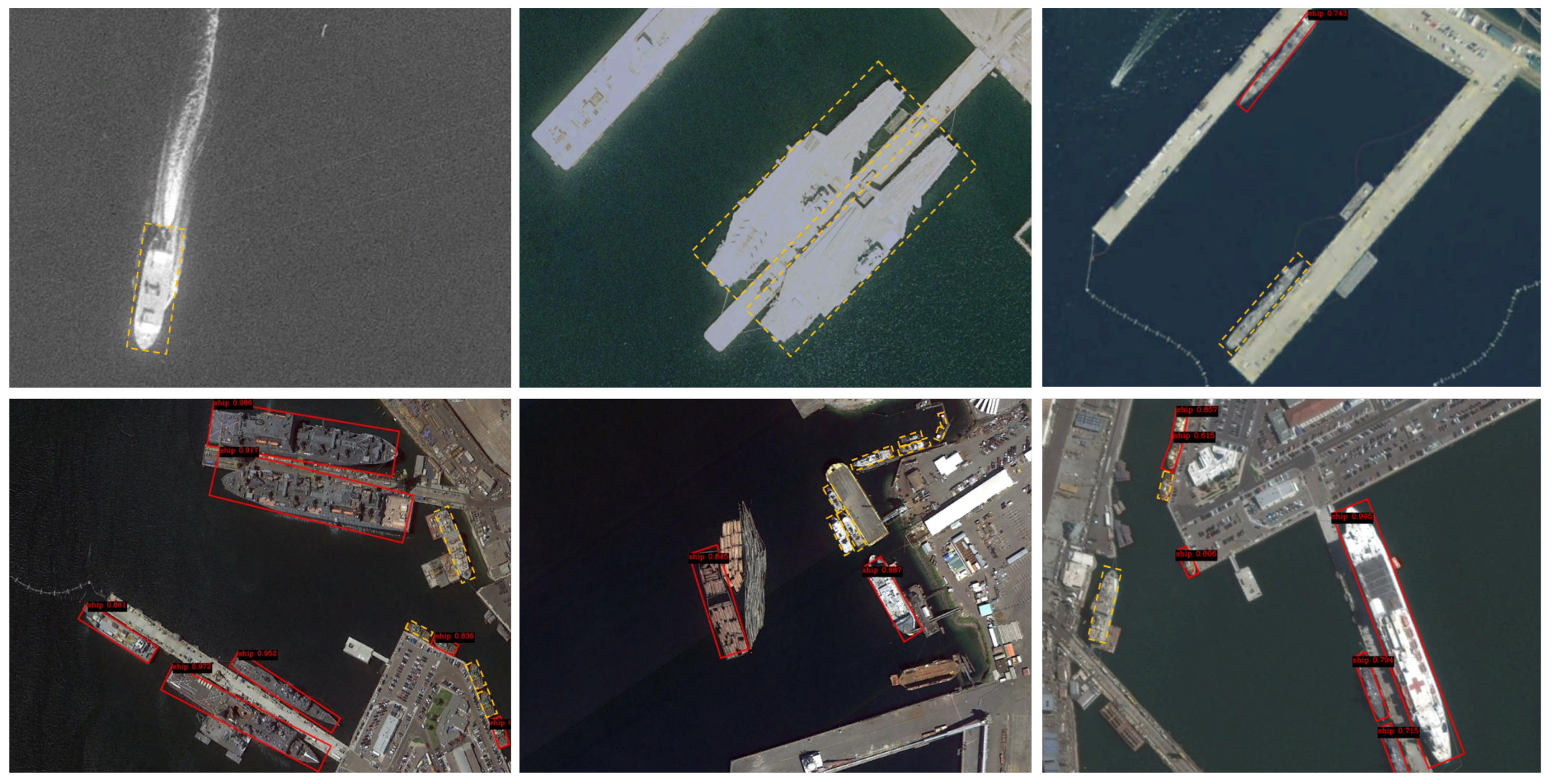
During our extensive testing phase, the ABP-Net demonstrated remarkable performance across a variety of remote sensing tasks. However, we identified specific scenarios where the detector’s efficacy was compromised, particularly in the detection of slender targets under low-visibility conditions and within complex maritime environments.

Failure cases in low-visibility maritime environments: As shown in the first row of Figure 14, we encountered several failure cases where the ABP-Net struggled to detect targets in low-visibility conditions, commonly found in maritime environments. The primary issues arose from the reduced contrast between the target and the background, leading to inaccurate bounding box predictions. For instance, in images with heavy sea fog or under poor illumination, the fine details of ships were often indistinguishable, resulting in a significant drop in detection accuracy.

Challenges in small target detection: Another set of failure cases pertains to the detection of the small targets shown in the last row of Figure 14. Despite the adaptive boundary perception capabilities of the ABP-Net, the model occasionally missed small objects, particularly when they were partially occluded or present at a great distance from the sensor. The limited resolution and the lack of distinguishing features of these small targets made it difficult for the model to generate accurate bounding boxes.

Upon analysis, the failure cases can be attributed to the inherent limitations of the model in handling extreme variations in target size and visibility. The S-S label assignment, while effective for most scenarios, might not sufficiently address the challenges posed by very small or low-contrast targets. Similarly, the R-R loss function, although robust for general cases, may not provide the necessary fine-tuning required for the model to learn from these hard-to-detect samples. Future work will integrate feature enhancement techniques specifically tailored for small targets to improve detection accuracy. Additionally, we will develop robustness against environmental interference to ensure reliable performance in various maritime conditions.

5. Conclusions

This article proposes a method of detecting objects that are high-width targets in remote sensing images, called ABP-Net. Through the following two stages of the strategy, the boundary perception ability of the detector is enhanced: the pre-training label allocation phase and the training stage. During the pre-training phase, the S-S method is designed. This method is designed to better capture the critical information of the target with the goal of better capturing the critical information of the target according to the width and height ratio of the target. In order to solve the problem of instability caused by the long target, we proposed the R-R method. This function enhances the boundary positioning perception by paying attention to low-error samples and inhibiting the gradient enlargement of difficult samples. We conducted experiments on UCAS-AOD and HRSC2016 datasets to verify the performance of our detectors specifically for high-width targets. The results show that our method improves the detection performance, efficiency, and accuracy when detecting high-width targets.